Spatio-temporal Characterization of Thermal Fluctuations in a Non-turbulent Rayleigh-Bénard Convection at Steady State
Abstract
In this paper we present a detailed description of the statistical and computational techniques that were employed to study a driven far-from-equilibrium steady-state Rayleigh-Bénard system in the non-turbulent regime (). In our previous work on the Rayleigh-Bénard convection system we try to answer two key open problems that are of great interest in contemporary physics: (i) how does an out-of-equilibrium steady-state differ from an equilibrium state and (ii) how do we explain the spontaneous emergence of stable structures and simultaneously interpret the physical notion of temperature when out-of-equilibrium. We believe that this paper will offer a useful repository of the technical details for a first principles study of similar kind. In addition, we are also hopeful that our work will spur considerable interest in the community which will lead to the development of more sophisticated and novel techniques to study far-from-equilibrium behavior.
I Introduction
The Rayleigh-Bénard convection system holds a place of special interest in the scientific community bodenschatz2000recent ; cross1993pattern ; behringer1985rayleigh . It is one of the oldest and most widely used canonical examples to study pattern formation and emergent behavior cross1993pattern ; koschmieder1993benard ; jaeger2010far ; heylighen2001science . The wide variety of conceptual richness offered by the Rayleigh-Bénard convection makes it an active area of research in the thermal, fluids and complexity science disciplines bodenschatz2000recent ; cross1993pattern ; koschmieder1993benard ; zhang1993deterministic ; shishkina2010boundary ; kadanoff2001turbulent . It is infact one of the simplest complex systems’ that can be easily recreated in a laboratory with minimal efforts. Although, the current state of the art experimental setups, data logging techniques, numerical and mechanistic simulations have provided numerous critical insights about the fluid mechanical aspects, a lot of the thermodynamical interpretations still remain unresolved niemela2000turbulent ; chilla2012new ; du2000turbulent ; du2001temperature ; pandey2018turbulent ; stevens2011prandtl . The simple idea that a thin film of viscous liquid when heated from the bottom at steady-state, gives rise to a plethora of emergent patterns that are stationary in time is inviting enough to invoke deep theoretical curiosities about the far-from-equilibrium interpretation of the (thermodynamic) equation of state lucia2008probability ; garcia2008thermodynamics ; gallavotti2019nonequilibrium ; chatterjee2016energy ; chatterjee2016thermodynamics ; yadati2018detailed ; lieb1998guide ; martyushev2006maximum ; chatterjee2013principle ; georgiev2016road . In a recent series of papers, we have outlined these open problems through a systematic thermodynamic study of a non-turbulent Rayleigh-Bénard convection system at steady-state chatterjee2018many ; chatterjee2018non ; 2018arXiv181206002C ; srinivasarao2019biologically . This paper serves as a repository of experimental details, computational and analytical techniques. We strongly believe that the ideas laid out in this paper will not only serve as an evidence of reproducibility but will also spur considerable interest in the search for more efficient and novel techniques in the study of far-from-equilibrium thermodynamics in the future.
Over the years the Rayleigh-Bénard system has seen many state-of-the-art developments which have successfully helped us understanding the fluid mechanical aspects of the system along with theoretical and computational insights in turbulence studies shishkina2010boundary ; du2000turbulent ; du2001temperature ; pandey2018turbulent ; stevens2011prandtl ; du1998enhanced ; stevens2010radial ; schumacher2008lagrangian ; grossmann2004fluctuations . However, from a first principles thermodynamic point of view this system has a lot of insights to offer which have largely gone unnoticed. In recent series of papers we have investigated as how the thermodynamics of a far-from-equilibrium steady-state differs that from an equilibrium state. We have tried to quantify and characterize the differences by studying out-from-equilibrium thermal fluctuations in a driven Rayleigh-Bénard system. In this paper, we present the computational and statistical details of our results with the hope that this will serve as a reference for all future works in this line of thinking chatterjee2018many ; 2018arXiv181206002C ; vilar2001thermodynamics ; lucia2013stationary .
II Experimental Methodology
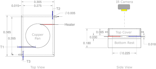
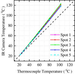
The strength of our work lies in our simplistic approach. In Figure 1 we present a detailed outline of our experimental setup. A thin layer of Silicone oil is heated in a copper pan 111For more information about the properties of the sample fluid please refer 2018arXiv181206002C ; shinetsu . A J-type thermocouple (T1) attached to the bottom of the copper pan measures its base temperature, . Copper being a good conductor of heat allows the flow of energy through it with minimal thermal resistance. The average diameter of the pan is . The pan is heated from the bottom by an electric resistance heater (). The top cover is made up of wood and has inlet and outlet ducts for forced convective heat transfer. The two thermocouples T2 and T3 measure the temperature of the incoming and outgoing gas respectively. The bottom rest, also made up of wood has a cavity with a recess on which the copper pan sits snugly. The wooden base rests on top of a block of polyurethane foam. An IR camera, placed concentrically above the copper pan captures the real-time thermal images from a height (). Each thermal image has its own temperature scale. In order to calibrate the IR camera with the base thermocouple (T1), the empty copper pan is heated and the temperature of five randomly chosen points on the copper pan are recorded at different power settings of the resistance heater at steady-state. The thermocouple temperature recorded by T1 is then compared with the IR camera recorded temperature for the five spots. The thermocouple data can be viewed in the NI Signal Express software while the IR camera data is viewed in the FLIR Software. The FLIR software allows remote accessibility like, real-time display, region/point selection and spatial statistics. In Figure 2, we present the calibration curves for the five spots comparing the IR camera-recorded temperature with the base thermocouple temperature. The calibration error thus estimated is used to adjust the IR camera temperature scale in accordance with the base thermocouple.
Once the IR camera is calibrated one can set up the system to perform a series of experiments to gather thermal data. A high viscosity silicone oil is used for the purpose of the current study 2018arXiv181206002C ; shinetsu . The fluid is placed in the copper pan and it is then heated by regulating the externally applied voltage. It is always ensured that a large pan diameter () to fluid-film thickness () is maintained, , as the goal is to have convection cells over as wide as an area possible for the thermal imaging to yield significant temperature statistics. It is also ensured that the applied power never exceeds a value that can change the molecular configuration of the oil through burning or render the system into a turbulent regime through boiling. Since, our study is focused within the non-turbulent regime, the Rayleigh Number, . For more details about the operational regime of the for the current scope of study please refer 2018arXiv181206002C .
III Image Analysis
An IR Camera detects heat emitted from an object and converts it into bits. Thus, every pixel has an allocated bit value between and . The bit value determines the intensity of the pixel with being the ‘coldest’ pixel in the image and being the most intense or the ‘hottest’. The FLIR T62101, used in this study has a resolution of pixels ( pixels) with a sensitivity less than C. Therefore, every image () is a 2D array () of elements with bit values distributed in between them. In this study, the IR camera is used to film the thermal profile of the top layer of the fluid-film. Using the IR camera temperature scale and the estimated calibration error, each of these bit values can be converted to respective temperature values through a linear interpolation as shown in 1.
| (1) |
Each entry in the matrix can now be denoted by a temperature with the pair defining a particular pixel location on the thermal image.
IV Results and Discussion
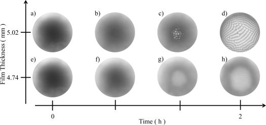
This paper aims to illustrate the experimental and statistical methodologies to quantify spatio-temporal thermal fluctuations in a driven out-of-equilibrium steady-state system. A steady-state is achieved at a particular power by letting the fluid sample to gradually evolve from a room temperature equilibrium to an out-of-equilibrium state after two hours of constant heating. The snapshots of the thermal images are obtained using the IR camera for every of a second thus yielding images over the total duration of two hours. In Figure 3, we present a sample of the snapshots of the Rayleigh-Bénard system at different instances in time for the two film-thicknesses at a fixed power of .
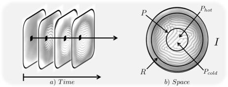
Each of these images are converted into a temperature matrix on which statistical analyses are performed by choosing regions of interest. To select a square or a rectangular region, the coordinates of the upper left edge and the coordinates of the lower right edge are specified. To select a circular or an annular region, the center point and radii (internal and external) are specified with constraints on the spatial location of the coordinates in the region of interest. In summary, we can isolate regions of interest in each of the thermal images and thus perform statistical analysis spatially to obtain descriptive statistics such as, mean, standard deviation, kurtosis etc. In Figure 4, we illustrate as an example plot the mean and standard deviation of an arbitrary region of the top film temperature as a function of time as the the Rayleigh-Bénard system evolves from room temperature equilibrium to an out-of-equilibrium steady-state. To better illustrate the analysis strategy we present a pictorial representation in Figure 5. In Figure 5a, a specific region of interest is followed in time in order to extract temporal statistics whereas, in Figure 5b, a region of interest is specified in a steady-state image in order to extract spatial statistics. The annular non-convective region is denoted by , whereas the pattern region by . The sub-regions within are denoted as and corresponding to updrafts (or upward plumes) and downdrafts (or downward plumes). For an arbitrary region on the top film the mean and standard deviation are calculated as, and .
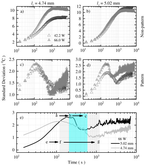
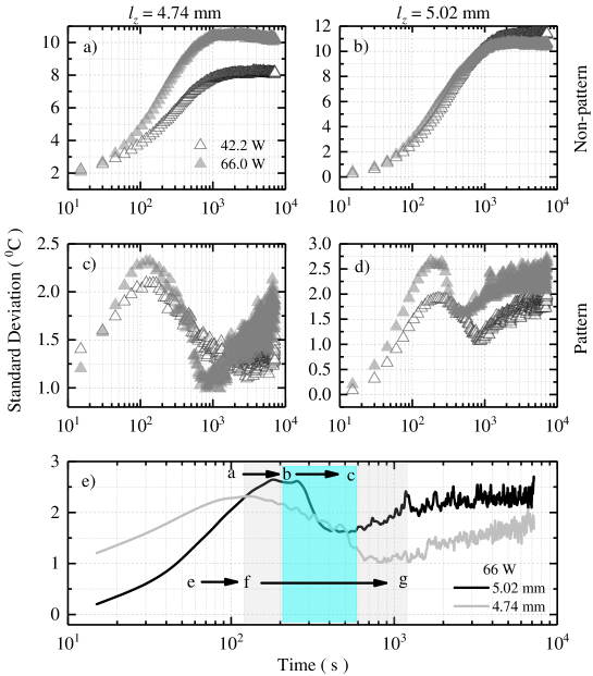
In Figure 6, we take our statistical analysis a step further by plotting the standard deviation of the temperature, a measure of the thermal fluctuation, as a function of time by isolating the pattern and non-pattern regions for the two thicknesses at and . We can see contrasting trends between Figure 6a and 6b. In Figure 6a and 6b, the standard deviation increases with time till saturation as the system reaches a steady-state. Whereas, in the case of the pattern region in Figure 6c and 6d, the standard deviation first shows a decline when the pattern starts to form but is not yet visible, followed by a dip at the point a stable visible pattern starts emerging. We further illustrate this in Figure 6e, where we compare the temporal evolution of the standard deviation of the temperature for the two thicknesses at . The shaded boxes in the plot identify the time windows when the standard deviation starts to decline and then increasing again. With increasing power we can observe that the standard deviation of the temperature grows in time and the time window for the standard deviation shortens as . For a thicker fluid film the time window is observed to be shorter as, . Thus, a critical local Rayleigh Number is achieved faster. One can also identify the beginning and the ending of the time window with the thermal image snapshot labels from Figure 3. The window in cyan identifies the transition from for , whereas the window in light grey identifies the transition from for . The images and are equilibrium snapshots (at ) taken for both the thicknesses respectively.
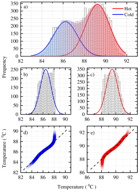
We perform spatial statistical analysis on our steady-state images, i.e. for a particular thickness at a fixed power, we choose the last image (snapshot taken after two hours). We isolate pattern and non-pattern regions by defining circular and annular regions of interest on the thermal images. Once the regions are specified, a 1D array is created to store the temperature values, at every pixel location. Once a 1D array of all temperature values, is obtained a frequency histogram is generated to model the distribution of temperature spatially for our regions of interest. In Figure 7a, we show the histogram distribution when our region of interest falls over the patterns in the thermal images. A clear bimodality is observed in the frequency histogram. We identify the two peaks and perform two independent Gaussian fits, on the data: for the ‘hot’ region (in red) and for the ‘cold’ region (in blue). The shaded region enclosing both the Gaussian fits is a cumulative fit function. We have shown in our previous works that a kernel density estimate provides a better description of the shape of the frequency data, . However, a kernel smoothening with Gaussian kernels () does not present any intuitive understanding of the physics beyond the shape of the estimate function. We identify the point where the two independent Gaussian fits intersect each other. We set the temperature at the point of intersection of the two curves as a threshold () to slice the frequency data into two regimes: ‘hot’ and ‘cold’. Two independent 1D arrays are created and the temperature frequency data is binned accordingly: if then the list of all is in ‘cold’ region and if then the list of all is in ‘hot’ region. We look at their independent statistics in Figure 7b and 7c. The histograms are clearly normally distributed with for the isolated ‘hot’ region and for the isolated ‘cold’ region. One can see that the descriptive statistics of the isolated regions is well within one standard deviation of the continuous region with CI. To further elucidate the normal behavior we show the Q-Q plots for the isolated regions in Figure 7d and 7e. One can clearly note that at the curves depart from normality whereas everywhere else they are in agreement with the normal nature of the frequency distribution. We discuss this idea in our previous work as the coexistence of multiple equilibrium points in an out-of-equilibrium steady-state system chatterjee2018many ; 2018arXiv181206002C .
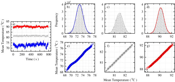
In our previous work we had claimed that the spatial symmetry is broken although temporal symmetry is preserved. In order to look at the temporal behavior of the Rayleigh-Bénard system at out-of-equilibrium steady-state, we let the system evolve beyond the steady-state () and capture a real-time video. For the purpose of this study a minute video was recorded at frames/second thus yielding frames. We show the time-series data in Figure 8a. To obtain robust temporal statistics, regions of interest were selected on the thermal images and were spatially averaged across frames. In Figure 8b, 8c, and 8d we plot the frequency histograms for the ‘hot’ (in red), ‘cold’ (in blue) and the whole region (in light grey). These histograms are clearly normally distributed: (red), (blue) and all at CI. The statistical mean of the whole region is found to be very close to the average of the statistical means of the respective ‘hot’ and the ‘cold’ regions. To further ascertain the normality of the frequency histograms, Q-Q plots are shown for the each of the regions of interest in Figure 8e, 8f, and 8g.
It is clear by now that the thermal profile of the top layer of the fluid film is non-uniform. In order to visualize the modulation in the temperature as a function of distance several line cuts are performed on the thermal images. These line cuts are constructed from the image matrix by choosing 1D arrays of row/column data. In Figure 9, we plot spatially averaged thermal profiles along six horizontal line cuts aligned parallel to each other.
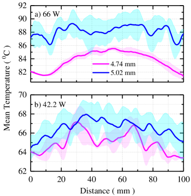
As expected, the mean temperature in Figure 9a is greater than the mean temperature in 9b. The modulation in the thermal profiles describe the thermal-field heterogeneity. The flatness of the thermal profile allows us to identify spatial correlation lengths of thermal fluctuations in the system. On comparing Figure 9a and 9b, it can be observed that at higher power () the thermal profiles tend to be more uniform over longer length-scales than at lower power (). There are two reasons for this observation. One, at lower power the pattern occupies a smaller area about the center while the majority of the peripheral region being ‘cooler’ thus implying more thermal heterogeneity as one approaches the periphery from the center, and two, at lower power the emergent patterns are not fully developed yet and hence randomly oriented. Thus, the modulation is uneven and hence chaotic. At higher power, the emergent patterns are fully developed and exhibit a closed packing thus being more homogeneous.
In order to reconstruct the complete geometry of the thermal field we need to extract the thermal profile and integrate over the whole region. In order to execute this, thermal profiles of normalized integrated intensities around concentric circles are plotted as a function of distance from a point in the image. This point of reference is defined by the center of the rectangle that bounds the region of interest. The position of this point can be modified by user defined commands. The temperature at any given distance from this point represents the sum of the pixel values around a circle, whose radius is the distance from the point. The integrated intensity is then divided by the number of pixels in the circle thus yielding normalized density values. This profile is plotted as a function of distance by defining a starting and an integration angle to perform a radial averaging. The radial averaging allows us to identify the distance between subsequent maxima and minima on the thermal field.
However, to extract meaningful length-scales from the entire thermal profile we need a more sophisticated technique. Therefore, we employ a spatial two-point autocorrelation to extract useful information about the emergent length scales from the system. It is done by comparing the frequencies of values in the temperature matrix, and then finding the most dominant frequencies. In this case, the autocorrelation function analyzes the 2D temperature profile matrix and finds correlations based on length, at an arbitrary delay, away from each element in the matrix. The program is written following the Weiner-Khinchin theorem which relates the autocorrelation function to the power spectral density via the Fourier transform wiener1930generalized ; mears2019stochastic . The 2D spatial autocorrelation is executed using Python’s numpy library. We make use of its 2D fast Fourier transform and its complex conjugate functions, fft.fft2 and conj. The matrix is normalized to a range of values . Numpy provides another useful function called fft.fftshift which moves the zero coordinate to the center of the domain. Implementing this outputs a much smoother autocorrelation function as output. In order to convert the 2D autocorrelation function into a 1D radius based autocorrelation, all the elements inside the circle of arbitrary radius around the center of the matrix are averaged and the normalized is plotted as a function of this delay in Figure 10. The spatial autocorrelation data is fitted with an exponential decay function, where is the correlation length. In Figure 10, we can see that there exists atleast two correlation lengths, and . The larger correlation length captures coarser (more uniform) length scales whereas the smaller one captures finer length scales. One can compare Figure 10 with Figure 9a to check for consistency and refer to the discussion presented there.
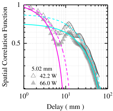
We saw in our previous discussion that a steady-state thermal profile has multiple emergent length-scales. In particular, it was observed in Figure 10 that there are atleast two dominant length-scales. When the Rayleigh-Bénard system is at room temperature equilibrium, it is thermodynamically homogeneous over large length-scales. Once, visible patterns emerge due to the system being driven out-of-equilibrium, finer length-scales start emerging on top of the intrinsic larger length-scale, as shown in Figure 10 and 11a. In our previous work we had discussed the connection between the emergence of the finer length-scales and the decline in the standard deviation of the temperature (see Figure 4 and 6) 2018arXiv181206002C . A question that naturally follows is how these typical length-scales are distributed (in time) as the system evolves from a room temperature equilibrium to an out-of-equilibrium steady-state. The spatial autocorrelation script is implemented on all the temperature matrices (or snapshots of the thermal images) while simultaneously fitting the spatial correlation data with exponential fits. The first data point of the spatial correlation dataset is always equal to one hence this point acts as an anchor for the first exponential fit. In order to obtain the second characteristic length, a search algorithm is implemented on the spatial correlation datset to search for a local minima followed by a local maxima. The local maxima acts as the anchor for the second exponential fit. It is also made sure that the second exponential fit undercuts the first exponential fit. The correlation length from the first exponential fit gives an estimate of the finer length-scales whereas, the second exponential fit gives an estimate of the larger (equilibrium or close to equilibrium) length scales in the system. The frequency histograms are then plotted as shown in Figure 11b. It is interesting to note that the larger length scales are lognormally distributed thus implying a positive skewness. Therefore, as the system ages (driven to a steady-state) finer length-scales emerge and a symmetrical normal distribution shifts towards the left. To put things into perspective of the system’s physical dimension, the smallest length-scale is estimated to be never less than and the largest length-scale is never greater than which is slightly above the radius of the copper pan.
V Conclusion
In this paper, we discuss thoroughly the computational and the statistical techniques that were employed to perform a first principles thermodynamic study on the non-turbulent steady-state Rayleigh-Bénard convection when driven out-of-equilibrium. The two key questions that form the basis of our previous studies are: (i) how does an out-of-equilibrium steady-state differ from an equilibrium state and (ii) how do we explain the spontaneous emergence of stable structures and simultaneously interpret the physical notion of temperature when out-of-equilibrium. We discuss in the very beginning of the paper our simplistic approach by laying out the details of the experimental setup. Thereafter, we discuss the details of the computational and statistical techniques. For the purpose of our analysis several programming software were used at different stages of the work like, C, Python, Matlab, ImageJ etc. From a statistical point of view, thorough descriptive statistical computations were performed to generate confidence intervals, linear and non-linear curve fittings were performed to model the large amount of experimental data and test goodness of fits. Image analysis techniques, like smoothening, parsing, slicing and matrix manipulations were also performed. We believe that this paper will add to the strength of our previous work by making it accessible and reproducible at the same time. We are very optimistic that this paper will serve as a repository of techniques, both experimental and computational, in advancing our knowledge about far-from-equilibrium thermodynamics.
VI Acknowledgment
The authors thank Prof. Germano Iannacchione in the Department of Physics at Worcester Polytechnic Institute for his critical feedback on the first draft of the paper. A.C. also expresses his gratitude towards the Department of Mathematical Sciences at Worcester Polytechnic Institute for arranging a meeting with Prof. Giovanni Gallavotti, which provided new insights about the theoretical aspects of the system concerning transport phenomenon and irreversibility.
References
- (1) E. Bodenschatz, W. Pesch, G. Ahlers, Recent developments in rayleigh-bénard convection, Annual review of fluid mechanics 32 (1) (2000) 709–778.
- (2) M. C. Cross, P. C. Hohenberg, Pattern formation outside of equilibrium, Reviews of Modern Physics 65 (3) (1993) 851.
- (3) R. Behringer, Rayleigh-benard convection and turbulence in liquid helium, Reviews of Modern Physics 57 (3) (1985) 657.
- (4) E. L. Koschmieder, Bénard cells and Taylor vortices, Cambridge University Press, 1993.
- (5) H. M. Jaeger, A. J. Liu, Far-from-equilibrium physics: An overview, arXiv preprint arXiv:1009.4874.
- (6) F. Heylighen, et al., The science of self-organization and adaptivity, The encyclopedia of life support systems 5 (3) (2001) 253–280.
- (7) D. Zhang, L. Györgyi, W. R. Peltier, Deterministic chaos in the belousov–zhabotinsky reaction: Experiments and simulations, Chaos: An Interdisciplinary Journal of Nonlinear Science 3 (4) (1993) 723–745.
- (8) O. Shishkina, R. J. Stevens, S. Grossmann, D. Lohse, Boundary layer structure in turbulent thermal convection and its consequences for the required numerical resolution, New journal of Physics 12 (7) (2010) 075022.
- (9) L. P. Kadanoff, Turbulent heat flow: structures and scaling, Physics Today 54 (8) (2001) 34–39.
- (10) J. Niemela, L. Skrbek, K. Sreenivasan, R. Donnelly, Turbulent convection at very high rayleigh numbers, Nature 404 (6780) (2000) 837.
- (11) F. Chillà, J. Schumacher, New perspectives in turbulent rayleigh-bénard convection, The European Physical Journal E 35 (7) (2012) 58.
- (12) Y.-B. Du, P. Tong, Turbulent thermal convection in a cell with ordered rough boundaries, Journal of Fluid Mechanics 407 (2000) 57–84.
- (13) Y.-B. Du, P. Tong, Temperature fluctuations in a convection cell with rough upper and lower surfaces, Physical Review E 63 (4) (2001) 046303.
- (14) A. Pandey, J. D. Scheel, J. Schumacher, Turbulent superstructures in rayleigh-bénard convection, Nature communications 9 (1) (2018) 2118.
- (15) R. J. Stevens, D. Lohse, R. Verzicco, Prandtl and rayleigh number dependence of heat transport in high rayleigh number thermal convection, Journal of Fluid Mechanics 688 (2011) 31–43.
- (16) U. Lucia, Probability, ergodicity, irreversibility and dynamical systems, in: Proceedings of the Royal Society of London A: Mathematical, Physical and Engineering Sciences, Vol. 464, The Royal Society, 2008, pp. 1089–1104.
- (17) V. García-Morales, J. Pellicer, J. A. Manzanares, Thermodynamics based on the principle of least abbreviated action: Entropy production in a network of coupled oscillators, Annals of Physics 323 (8) (2008) 1844–1858.
- (18) G. Gallavotti, Nonequilibrium thermodynamics, arXiv preprint arXiv:1901.08821.
- (19) A. Chatterjee, Energy, entropy and complexity: Thermodynamic and information-theoretic perspectives on ageing, M. Kyriazis (2016) Challenging Ageing: The anti-senescence effects of Hormesis, Environmental Enrichment, and Information Exposure. Bentham Science.
- (20) A. Chatterjee, Thermodynamics of action and organization in a system, Complexity 21 (S1) (2016) 307–317.
- (21) Y. Yadati, S. McGrath, A. Chatterjee, G. Georgiev, G. Iannacchione, A detailed thermodynamic study of rayleigh-benard cells, Bulletin of the American Physical Society (BAPS) Abstract: K47.00001.
- (22) E. H. Lieb, J. Yngvason, A guide to entropy and the second law of thermodynamics, in: Statistical Mechanics, Springer, 1998, pp. 353–363.
- (23) L. M. Martyushev, V. D. Seleznev, Maximum entropy production principle in physics, chemistry and biology, Physics reports 426 (1) (2006) 1–45.
- (24) A. Chatterjee, Principle of least action and convergence of systems towards state of closure, International Journal of Physical Research 1 (1) (2013) 21–27.
- (25) G. Y. Georgiev, A. Chatterjee, The road to a measurable quantitative understanding of self-organization and evolution, in: Evolution and Transitions in Complexity, Springer, 2016, pp. 223–230.
- (26) A. Chatterjee, G. Iannacchione, The many faces of far-from-equilibrium thermodynamics: Deterministic chaos, randomness, or emergent order?, MRS Bulletin 44 (2) (2019) 130–133. doi:10.1557/mrs.2019.18.
- (27) A. Chatterjee, G. Iannacchione, Non-equilibrium thermodynamics from first principles, Bulletin of the American Physical Society (BAPS) Abstract: Y47.00001.
- (28) A. Chatterjee, Y. Yadati, N. Mears, G. Iannacchione, Coexisting Ordered States, Local Equilibrium Points, and Broken Ergodicity in a Non-turbulent Rayleigh-Bénard Convection at Steady-state, arXiv e-prints (2018) arXiv:1812.06002arXiv:1812.06002.
- (29) M. Srinivasarao, G. S. Iannacchione, A. N. Parikh, Biologically inspired far-from-equilibrium materials, MRS Bulletin 44 (2) (2019) 91–95.
- (30) Y.-B. Du, P. Tong, Enhanced heat transport in turbulent convection over a rough surface, Physical Review Letters 81 (5) (1998) 987.
- (31) R. J. Stevens, R. Verzicco, D. Lohse, Radial boundary layer structure and nusselt number in rayleigh–bénard convection, Journal of Fluid Mechanics 643 (2010) 495–507.
- (32) J. Schumacher, Lagrangian dispersion and heat transport in convective turbulence, Physical Review Letters 100 (13) (2008) 134502.
- (33) S. Grossmann, D. Lohse, Fluctuations in turbulent rayleigh–bénard convection: the role of plumes, Physics of Fluids 16 (12) (2004) 4462–4472.
- (34) J. M. Vilar, J. Rubi, Thermodynamics “beyond” local equilibrium, Proceedings of the National Academy of Sciences 98 (20) (2001) 11081–11084.
- (35) U. Lucia, Stationary open systems: A brief review on contemporary theories on irreversibility, Physica A: Statistical Mechanics and its Applications 392 (5) (2013) 1051–1062.
- (36) For more information about the properties of the sample fluid please refer 2018arXiv181206002C ; shinetsu .
- (37) Shin Etsu Silicone-Global, http://www.shinetsusilicone-global.com/catalog/.
- (38) N. Wiener, et al., Generalized harmonic analysis, Acta mathematica 55 (1930) 117–258.
- (39) N. E. Mears, Stochastic simulations of far-from-equilibrium thermodynamics.