A Stochastic Gradient Method with Mesh Refinement for PDE Constrained Optimization under Uncertainty

Abstract

Models incorporating uncertain inputs, such as random forces or material parameters, have been of increasing interest in PDE-constrained optimization. In this paper, we focus on the efficient numerical minimization of a convex and smooth tracking-type functional subject to a linear partial differential equation with random coefficients and box constraints. The approach we take is based on stochastic approximation where, in place of a true gradient, a stochastic gradient is chosen using one sample from a known probability distribution. Feasibility is maintained by performing a projection at each iteration. In the application of this method to PDE-constrained optimization under uncertainty, new challenges arise. We observe the discretization error made by approximating the stochastic gradient using finite elements. Analyzing the interplay between PDE discretization and stochastic error, we develop a mesh refinement strategy coupled with decreasing step sizes. Additionally, we develop a mesh refinement strategy for the modified algorithm using iterate averaging and larger step sizes. The effectiveness of the approach is demonstrated numerically for different random field choices.

1 Introduction

In this paper, we are concerned with the numerical solution of a convex optimization problem with convex constraints and an elliptic partial differential equation (PDE) subject to uncertainty. In applications, the material coefficients and external inputs might not be known exactly. They can then be modeled to be distributed according to a known probability distribution. When the number of possible scenarios in the probability space is small, then the optimization problem can be solved over the entire set of scenarios. This approach is not relevant for most applications, as it becomes intractable if the source of uncertainty contains more than a few scenarios. Solvers for problems with random PDEs generally use either a discretization of the stochastic space or rely on sampling. Methods with a discretized stochastic space include the stochastic Galerkin method [6] and sparse-tensor discretization [34]. Sample-based approaches involve taking random or carefully chosen realizations of the input parameters; these approaches include Monte Carlo or quasi Monte Carlo methods and stochastic collocation [5].

In PDE-constrained optimization under uncertainty, there are several main algorithmic approaches. Most approaches involve using deterministic optimization methods in combination with a sampling or discretization scheme for the stochastic space. Stochastic collocation has been combined with multi-grid methods [7], gradient descent and SQP methods [35], and a trust region method [21]. In combination with sparse-grid collocation or low-rank tensors, trust-region methods have been proposed [22, 12]. Discretization of both spatial and stochastic spaces have been proposed in [19], and with a one-shot approach with stochastic Galerkin finite elements in [33]. All of these methods suffer from the curse of dimensionality – as the stochastic dimension increases, the number of quadrature points must increase exponentially.

Sample average approximation, also known as the Monte Carlo method, involves replacing the stochastic integral with a fixed sample of randomly chosen points. While the error in a Monte Carlo estimator decreases as $\mathcal{O}(1/\sqrt{N})$, where $N$ is the number of sampled points, this rate is independent of the stochastic dimension. There are known improvements to substantially improve the slow convergence of this method that have been developed for this problem class, including the multilevel Monte Carlo method [3] or the quasi Monte Carlo method [16]. In the context of approaches independent of the stochastic dimension, it is also worth mentioning the work of [2] and a following work [10], which is fundamentally different from the above approaches; this approach relies on Taylor expansions with respect to the parameter of the parameter-to-objective map.

Recently, stochastic approximation methods have been investigated for efficiently solving PDE-constrained optimization problems involving uncertainty [17, 26, 13]. This approach has previously been unexploited for PDE-constrained optimization, even though it is a classical method for solving stochastic optimization problems dating back to the 1950s [32, 20]. The main tool in stochastic approximation is a stochastic gradient, in place of the true gradient, to iteratively minimize the expected value over a random function. This method differs from the approaches mentioned above in that it is a fundamentally random method; sampling is performed in the course of the optimization procedure, rather than in addition to it. Like sample average approximation, it enjoys convergence rates independent of the stochastic dimension. In [17], the authors compare the stochastic approximation approach with the sample average approximation method for a fully discrete (both spatially and stochastically) PDE-constrained optimization problem, but they do not handle additional constraints or PDE discretization error. A mesh refinement strategy was presented in [26], but only in combination with step sizes of the form $c/n$; additionally, their results do not handle the case with additional constraints or with iterate averaging. Convergence theory with additional constraints in Hilbert spaces was presented in [13] along with a summary of step size rules, both for strongly convex and generally convex objective functionals; however, PDE discretization error was not handled in this work. In this work, we will extend the results in [13] to incorporate bias by PDE discretization error. We will see that we can obtain the same convergence theory, with the same expected error decay, if the discretization accuracy is steered such that the bias decays fast enough.

Relying on a priori error estimate for the discretization error, we provide a rule how the maximal mesh size should be coupled with the iteration progress. Analogously, one could couple the iteration with some a posteriori error measure, which has been well investigated for deterministic PDE-constrained optimization problems, see, e.g., [30, 31], and including the treatment of inexact discrete solutions [27].

The paper is structured as follows. In section 2, the algorithm and notation is presented. In section 3, efficiency estimates are derived for different step sizes choices. An application to PDE-constrained optimization is introduced in section 4, and a discretized version of the algorithm is presented. The presented version allows the coupling of step size rules to successive mesh refinement. Convergence orders for the algorithm are presented in Theorem 4.7, which is our main result. Experiments supporting the theoretical work are in section 5, and we close with final remarks in section 6.

2 Preliminaries

We consider problems of the form

$$\min_{u\in\mathcal{U}^{\text{ad}}}\left\{j(u)=\mathbb{E}[J(u,\xi)]=\int_{\Omega}J(u,\xi(\omega))\mathop{}\!\mathrm{d}\mathbb{P}(\omega)\right\},$$ (2.1)

where $\mathcal{U}^{\text{ad}}$ is a nonempty, closed, and convex subset of a Hilbert space $(\mathcal{U},(\cdot,\cdot)_{\mathcal{U}})$. We recall that a probability space is given by a triple $(\Omega,\mathcal{F},\mathbb{P})$, where $\Omega$ represents the sample space, $\mathcal{F}\subset 2^{\Omega}$ is the $\sigma$-algebra of events and $\mathbb{P}\colon\Omega\rightarrow[0,1]$ is a probability measure defined on $\Omega$. For the random vector $\xi:\Omega\rightarrow\Xi\subset\mathbb{R}^{m}$, we will often denote a realization of the random vector as simply $\xi\in\Xi.$ It is assumed that for almost every $\omega$, $u\mapsto J(u,\xi(\omega))$ is convex on $\mathcal{U}^{\text{ad}}$, making $j$ convex as well. Additionally, we require that $J:\mathcal{U}\times\Xi\rightarrow\mathbb{R}$ is $L^{2}$-Fréchet differentiable on an open neighborhood of $\mathcal{U}^{\text{ad}}$ according to the following definition, where $L^{p}(\Omega)$ denotes the space of all $p$-times integrable real-valued functions with norm $\lVert f\rVert_{L^{p}(\Omega)}=(\int_{\Omega}|f(\omega)|^{p}\mathop{}\!\mathrm{d}\mathbb{P}(\omega))^{1/p}$ and $\lVert\cdot\rVert_{\mathcal{U}}=\sqrt{(\cdot,\cdot)_{\mathcal{U}}}$ denotes the (strictly convex) norm on $\mathcal{U}$.

For the convenience of the reader, we recall the following definition from [13].

Definition 2.1.

A $p$-times integrable random functional $J:\mathcal{U}\times\Xi\rightarrow\mathbb{R}$ is called $L^{p}$-Fréchet differentiable at $u$ if for an open set $U\subset\mathcal{U}$ containing $u$ there exists a bounded and linear random operator $A:U\times\Xi\rightarrow\mathbb{R}$ such that $\lim_{h\rightarrow 0}\lVert J(u+h,\xi)-J(u,\xi)+A(u,\xi)h\rVert_{L^{p}(\Omega)}/\lVert h\rVert_{\mathcal{U}}=0$.

By Hölder’s inequality, if $u\mapsto J(u,\cdot)$ is $L^{p}$-differentiable and $1\leq r<p$, then it is also $L^{r}$-differentiable with the same derivative. This implies that $j:\mathcal{U}\rightarrow\mathbb{R}$ is Fréchet differentiable.

The projection onto a closed convex set $\mathcal{U}^{\text{ad}}\subset\mathcal{U}$ is denoted by $\pi_{\mathcal{U}^{\text{ad}}}:\mathcal{U}\rightarrow\mathcal{U}^{\text{ad}}$ and is defined as the function such that

$$\pi_{\mathcal{U}^{\text{ad}}}(u)=\underset{w\in\mathcal{U}^{\text{ad}}}{\operatorname*{arg\,min}}\,\lVert u-w\rVert_{\mathcal{U}}.$$

The projected stochastic gradient (PSG) method, which is studied in this paper, is summarized in Algorithm 1. It relies on a stochastic gradient, or a function $G:\mathcal{U}\times\Xi\rightarrow\mathcal{U}$ such that $G(u,\xi)\approx\nabla\mathbb{E}[J(u,\xi)]$; one choice for $G(u,\xi)$ is $\nabla_{u}J(u,\xi)$.

1:  Initialization: $u^{1}\in\mathcal{U}$

2:  for $n=1,2,\dots$ do

3:     Generate $\xi^{n}$, independent from $\xi^{1},\dots,\xi^{n-1}$, and $t_{n}>0$.

4:     $u^{n+1}:=\pi_{\mathcal{U}^{\text{ad}}}(u^{n}-{t_{n}}G(u^{n},\xi^{n}))$.

5:  end for

Algorithm 1 Projected Stochastic Gradient (PSG) Method

We recall that a sequence $\{\mathcal{F}_{n}\}$ of increasing sub-$\sigma$-algebras of $\mathcal{F}$ is called a filtration. A stochastic process $\{\beta_{n}\}$ is said to be adapted to the filtration if $\beta_{n}$ is $\mathcal{F}_{n}$-measurable for all $n$. If

$$\mathcal{F}_{n}=\sigma(\beta_{1},\dots,\beta_{n}),$$

we call $\{\mathcal{F}_{n}\}$ the natural filtration. Furthermore, we define for an integrable random variable $\beta:\Omega\rightarrow\mathbb{R}$ the conditional expectation $\mathbb{E}[\beta|\mathcal{F}_{n}]$, which is itself a random variable that is $\mathcal{F}_{n}$-measurable and satisfies $\int_{A}\mathbb{E}[\beta(\omega)|\mathcal{F}_{n}]\mathop{}\!\mathrm{d}\mathbb{P}(\omega)=\int_{A}\beta(\omega)\mathop{}\!\mathrm{d}\mathbb{P}(\omega)$ for all $A\in\mathcal{F}_{n}$.

We make the similar assumptions on the gradient as [13]; for the purposes of this paper, we will focus on the case where $\mathcal{U}^{\text{ad}}$ is bounded.

Assumption 2.2.

Let $\{\mathcal{F}_{n}\}$ be an increasing sequence of $\sigma$-algebras and the sequence of stochastic gradients generated by Algorithm 1 be given by $\{G(u^{n},\xi^{n})\}$. For each $n$, there exist $r^{n}$, $w^{n}$ with

$$r^{n}=\mathbb{E}[G(u^{n},\xi^{n})|\mathcal{F}_{n}]-\nabla j(u^{n}),\quad w^{n}=G(u^{n},\xi^{n})-\mathbb{E}[G(u^{n},\xi^{n})|\mathcal{F}_{n}],$$

which satisfy the following assumptions: (i) $u^{n}$ and $r^{n}$ are $\mathcal{F}_{n}$-measurable; (ii) $K_{n}:=\operatorname*{ess\,sup}_{\omega\in\Omega}\lVert r^{n}(\omega)\rVert_{\mathcal{U}}$ is bounded, i.e., $\sup_{n}K_{n}<\infty$; (iii) there exists a constant $M>0$ such that $\mathbb{E}[\lVert G(u,\xi)\rVert_{\mathcal{U}}^{2}]\leq M$ for all $u\in\mathcal{U}^{\text{ad}}.$

Notice that by construction, $\mathbb{E}[w^{n}|\mathcal{F}_{n}]=0$ and hence no further assumptions on $w^{n}$ are needed.

3 Efficiency Estimates for Stochastic Gradient Methods

To obtain efficiency estimates, we let $u$ be an optimal solution of (2.1) and $g^{n}=G(u^{n},\xi^{n})$. Since $u\in\mathcal{U}^{\text{ad}}$, $\pi_{\mathcal{U}^{\text{ad}}}(u)=u.$ Thus, the nonexpansivity of the projection operator yields

$$\lVert u^{n+1}-u\rVert_{\mathcal{U}}^{2} =\lVert\pi_{\mathcal{U}^{\text{ad}}}(u^{n}-t_{n}g^{n})-\pi_{\mathcal{U}^{\text{ad}}}(u)\rVert_{\mathcal{U}}^{2}$$ (3.1)

$$\leq\lVert u^{n}-t_{n}g^{n}-u\rVert_{\mathcal{U}}^{2}$$

$$=\lVert u^{n}-u\rVert_{\mathcal{U}}^{2}-2t_{n}(u^{n}-u,g^{n})_{\mathcal{U}}+t_{n}^{2}\lVert g^{n}\rVert_{\mathcal{U}}^{2}.$$

Since $\xi^{n}$ is independent from $\xi^{1},\dots,\xi^{n-1}$, it follows that

$$\mathbb{E}[\lVert g^{n}\rVert_{\mathcal{U}}^{2}|\mathcal{F}_{n}]=\mathbb{E}[\lVert G(u^{n},\xi)\rVert_{\mathcal{U}}^{2}]\leq M.$$ (3.2)

By Assumption 2.2, $g^{n}=\nabla j(u^{n})+w^{n}+r^{n}.$ Since $u^{n}$ and $r^{n}$ are $\mathcal{F}_{n}$-measurable, it follows that $\mathbb{E}[u^{n}|\mathcal{F}_{n}]=u^{n}$ and $\mathbb{E}[r^{n}|\mathcal{F}_{n}]=r^{n}$. Note as well that $\mathbb{E}[w^{n}|\mathcal{F}_{n}]=0$ holds. Thus taking conditional expectation with respect to $\mathcal{F}_{n}$ on both sides of (3.1), we get

$$\mathbb{E}[\lVert u^{n+1}-u\rVert_{\mathcal{U}}^{2}|\mathcal{F}_{n}]\leq\lVert u^{n}-u\rVert_{\mathcal{U}}^{2}-2t_{n}(u^{n}-u,\nabla j(u^{n})+r^{n})_{\mathcal{U}}+t_{n}^{2}M.$$ (3.3)

In the following computations, let $e_{n}^{2}:=\mathbb{E}[\lVert u^{n}-u\rVert_{\mathcal{U}}^{2}]$.

3.1 Strongly Convex Case

Notice that

$$-2t_{n}(u^{n}-u,r^{n})_{\mathcal{U}}\leq 2t_{n}(\lVert u^{n}-u\rVert_{\mathcal{U}}^{2}+1)\lVert r^{n}\rVert_{\mathcal{U}}$$

and the $\mu$-strong convexity of $j$ implies that $(u^{n}-u,\nabla j(u^{n}))_{\mathcal{U}}\geq\mu\lVert u^{n}-u\rVert_{\mathcal{U}}^{2}$. Hence, taking expectation on both sides of (3.3), we obtain

$$e_{n+1}^{2}\leq e_{n}^{2}(1-2\mu t_{n}+2t_{n}K_{n})+t_{n}^{2}M+2t_{n}K_{n}.$$

To ensure convergence of $\{e_{n}^{2}\}$, we require that $\sum_{n}t_{n}K_{n}<\infty$ and $\sum_{n}t_{n}^{2}<\infty$; see [13, Theorem 3.6]. We use for some later to be determined $K,\nu,\theta>0$ the ansatz

$$K_{n}\leq\frac{K}{n+\nu},\quad t_{n}=\frac{\theta}{n+\nu},$$ (3.4)

resulting in the inequality

$$e_{n+1}^{2}\leq e_{n}^{2}\left(1-\frac{2\mu\theta}{n+\nu}+\frac{2\theta K}{(n+\nu)^{2}}\right)+\frac{\theta^{2}M+2\theta K}{(n+\nu)^{2}}.$$ (3.5)

Lemma 3.1.

For a recursion of the form

$$e_{n+1}^{2}\leq e_{n}^{2}\left(1-\frac{c_{1}}{n+\nu}+\frac{c_{2}}{(n+\nu)^{2}}\right)+\frac{c_{3}}{(n+\nu)^{2}},$$ (3.6)

if $e_{1}^{2},c_{2},c_{3}\geq 0$, $c_{1}>1$, and $\nu+1\geq\frac{c_{2}}{c_{1}-1}$, it follows that

$$e_{n}^{2}\leq\frac{\rho}{n+\nu},$$ (3.7)

where

$$\rho:=\max\Big{\{}(1+\nu)e_{1}^{2},\frac{-c_{3}(1+\nu)}{(1+\nu)(1-c_{1})+c_{2}}\Big{\}}.$$

Proof.

We show (3.7) by induction. The statement for $n=1$ is clearly satisfied since $e_{1}^{2}=\frac{\nu+1}{\nu+1}e_{1}^{2}\leq\frac{\rho}{\nu+1}.$

For $n>1$, we assume that (3.7) holds for $n$. We abbreviate $\hat{n}:=n+\nu$ and since $\nu+1\geq\frac{c_{2}}{c_{1}-1}$, we have

$$1-\frac{c_{1}}{\hat{n}}+\frac{c_{2}}{\hat{n}^{2}}>0.$$

Thus by (3.6) and (3.7), we get

$$e_{n+1}^{2} \leq\left(1-\frac{c_{1}}{\hat{n}}+\frac{c_{2}}{\hat{n}^{2}}\right)\frac{\rho}{\hat{n}}+\frac{c_{3}}{\hat{n}^{2}}$$ (3.8)

$$=\left(\frac{\hat{n}^{2}-\hat{n}}{\hat{n}^{3}}\right)\rho+\left(\frac{\hat{n}(1-c_{1})+c_{2}}{\hat{n}^{3}}\right)\rho+\frac{c_{3}}{\hat{n}^{2}}$$

$$\leq\frac{\rho}{\hat{n}+1}.$$

In the last inequality, we used the fact that $\hat{n}^{3}\geq\hat{n}(\hat{n}-1)(\hat{n}+1)$ and the fact that for all $n\in\mathbb{N}$ and $\hat{n}=n+\nu$, the relation

$$\left(\frac{\hat{n}(1-c_{1})+c_{2}}{\hat{n}^{3}}\right)\rho+\frac{c_{3}}{\hat{n}^{2}}\leq\left(\frac{\hat{n}(1-c_{1})+c_{2}}{\hat{n}^{3}}\right)\frac{-c_{3}(1+\nu)}{(\nu+1)(1-c_{1})+c_{2}}+\frac{c_{3}}{\hat{n}^{2}}$$

is true, since the factor in front of $\rho$ is negative by assumption on $\nu$, i.e., $(\nu+1)(1-c_{1})+c_{2}\leq 0$. Further, we calculate

$$\left(\frac{\hat{n}(1-c_{1})+c_{2}}{\hat{n}^{3}}\right)\frac{-c_{3}(1+\nu)}{(1+\nu)(1-c_{1})+c_{2}}+\frac{c_{3}}{\hat{n}^{2}} \leq 0$$

$$\Leftrightarrow-c_{3}(1+\nu)[(n+\nu)(1-c_{1})+c_{2}] \geq-c_{3}(n+\nu)[(1+\nu)(1-c_{1})+c_{2}]$$

$$\Leftrightarrow(1+\nu) \leq(n+\nu),$$

thus showing (3.8). ∎

Summarizing the above derivation, we obtain the following convergence theorem.

thm 3.2.

If $j$ is $\mu$-strongly convex and $\theta$ and $\nu$ are chosen such that $\theta>1/(2\mu)$ and $\nu\geq 2\theta K/(2\mu\theta-1)-1$, then

$$\mathbb{E}[\lVert u^{n}-u\rVert_{\mathcal{U}}]\leq\sqrt{\frac{\rho}{n+\nu}}$$ (3.9)

with

$$\rho:=\max\left\{(1+\nu)\mathbb{E}[\lVert u^{1}-u\rVert_{\mathcal{U}}^{2}],\frac{-(\theta^{2}M+2\theta K)(1+\nu)}{(1+\nu)(1-2\mu\theta)+2\theta K}\right\}.$$

If additionally, $\nabla j$ is Lipschitz continuous with constant $L>0$ and $\nabla j(u)=0$, then

$$\mathbb{E}[j(u^{n})-j(u)]\leq\frac{L\rho}{2(n+\nu)}.$$ (3.10)

Proof.

The estimate (3.9) is an immediate consequence of (3.5) and Lemma 3.1. If $\nabla j$ is Lipschitz continuous and $\nabla j(u)=0$, then it follows that

$$j(u^{n})\leq j(u)+\frac{L}{2}\lVert u^{n}-u\rVert_{\mathcal{U}}^{2},$$ (3.11)

so combining (3.11) with (3.9), we get (3.10). ∎

3.2 Convex Case with Averaging

In the general convex case, or where a good estimate for $\mu$ does not exist, step sizes of the form $t_{n}=\theta/n$ may be too small for efficient convergence. An example is given in [28] showing that an overestimated strong convexity parameter $\mu$ leads to extremely slow convergence. A significant improvement can be obtained by using larger steps of the order $\mathcal{O}(1/\sqrt{n})$. Then, instead of observing convergence of the sequence $\{u^{n}\}$ we observe the convergence of certain averages $\tilde{u}_{i}^{N}$ of the iterates, with $\gamma_{n}:=t_{n}/(\sum_{\ell=i}^{N}t_{\ell})$ and the average of the iterates for some choice of $i$ to $N$ given by

$$\tilde{u}_{i}^{N}=\sum_{n=i}^{N}\gamma_{n}u^{n}.$$ (3.12)

To derive these estimates, we use (3.3) and the fact that $(u^{n}-u,\nabla j(u^{n}))_{\mathcal{U}}\geq j(u^{n})-j(u)$ by convexity of $j$ to get a recursion of the form

$$e_{n+1}^{2} \leq e_{n}^{2}(1+2t_{n}K_{n})-2t_{n}\mathbb{E}[j(u^{n})-j(u)]+t_{n}^{2}M+2t_{n}K_{n}.$$ (3.13)

Rearranging (3.13) and summing over $1\leq i\leq N$ on both sides,

$$\sum_{n=i}^{N}t_{n}\mathbb{E}[j(u^{n})-j(u)] \leq\sum_{n=i}^{N}\left[\frac{e_{n}^{2}}{2}(1+2t_{n}K_{n})-\frac{e_{n+1}^{2}}{2}+\frac{t_{n}^{2}M}{2}+t_{n}K_{n}\right]$$ (3.14)

$$\leq\frac{e_{i}^{2}}{2}+\frac{1}{2}\sum_{n=i}^{N}\left[2t_{n}K_{n}e_{n}^{2}+t_{n}^{2}M+2t_{n}K_{n}\right].$$

By convexity of $j$, we have $j(\tilde{u}_{i}^{N})\leq\sum_{n=i}^{N}\gamma_{n}j(u^{n})$ so by (3.14)

$$\mathbb{E}[j(\tilde{u}_{i}^{N})-j(u)]\leq\frac{e_{i}^{2}+\sum_{n=i}^{N}[2t_{n}K_{n}e_{n}^{2}+t_{n}^{2}M+2t_{n}K_{n}]}{2\sum_{n=i}^{N}t_{n}}.$$ (3.15)

Set $D_{\text{ad}}:=\sup_{u\in\mathcal{U}^{\text{ad}}}\lVert u_{1}-u\rVert_{\mathcal{U}}$. Notice that $e_{1}^{2}\leq D_{\text{ad}}^{2}$ and $e_{i}^{2}\leq 4D_{\text{ad}}^{2}$ since $\lVert u_{i}-u\rVert_{\mathcal{U}}\leq\lVert u_{i}-u_{1}\rVert_{\mathcal{U}}+\lVert u_{1}-u\rVert_{\mathcal{U}}\leq 2D_{\text{ad}}$. Thus from (3.15) we get

$$\mathbb{E}[j(\tilde{u}_{1}^{N})-j(u)] \leq\frac{D_{\text{ad}}^{2}+\sum_{n=1}^{N}\left[8t_{n}K_{n}D_{\text{ad}}^{2}+t_{n}^{2}M+2t_{n}K_{n}\right]}{2\sum_{n=1}^{N}t_{n}},$$ (3.16)

$$\mathbb{E}[j(\tilde{u}_{i}^{N})-j(u)] \leq\frac{4D_{\text{ad}}^{2}+\sum_{n=i}^{N}\left[8t_{n}K_{n}D_{\text{ad}}^{2}+t_{n}^{2}M+2t_{n}K_{n}\right]}{2\sum_{n=i}^{N}t_{n}},\quad 1<i\leq N.$$ (3.17)

If $K_{n}=0$, then we recover the estimates [28, (2.18)].

Constant Step Size Policy

First, observe the case where $t_{n}=t$ and $i=1$. It follows by (3.16) that

$$\mathbb{E}[j(\tilde{u}_{1}^{N})-j(u)]\leq\frac{D_{\text{ad}}^{2}+\sum_{n=1}^{N}\left[8tK_{n}D_{\text{ad}}^{2}+t^{2}M+2tK_{n}\right]}{2Nt}$$

Minimizing $f(t):=(D_{\text{ad}}^{2}+\sum_{n=1}^{N}\left[8tK_{n}D_{\text{ad}}^{2}+t^{2}M+2tK_{n}\right])/(2Nt)$, we get the step size policy

$$t=\frac{D_{\text{ad}}}{\sqrt{MN}},$$ (3.18)

which is the same step size rule as one would use where $K_{n}=0.$ Plugging (3.18) into (3.16), we get

$$\mathbb{E}[j(\tilde{u}_{1}^{N})-j(u)]\leq\frac{D_{\text{ad}}\sqrt{M}}{\sqrt{N}}+\frac{4D_{\text{ad}}^{2}+1}{N}\sum_{n=1}^{N}K_{n}.$$

Hence for convergence with the same speed as in the case $K_{n}=0$ it is sufficient that

$$\sum_{n=1}^{N}K_{n}\propto\sqrt{N}.$$ (3.19)

Variable Step Size Policy

Alternatively, one can work with the decreasing step size policy for a constant $\theta>0$

$$t_{n}=\frac{\theta D_{\text{ad}}}{\sqrt{Mn}}.$$ (3.20)

Plugging (3.20) into (3.17), we get using the inequalities

$$\sum_{n=i}^{N}\frac{1}{n}\leq\frac{N-i+1}{i},\quad\sum_{n=i}^{N}\frac{1}{\sqrt{n}}\geq\frac{N-i+1}{\sqrt{N}}$$

the following estimate for $1\leq i\leq N$

$$\quad\mathbb{E}[j(\tilde{u}_{i}^{N})-j(u)]\leq\frac{1}{\sqrt{N}}\left[\frac{2D_{\text{ad}}N\sqrt{M}}{\theta(N-i+1)}+\frac{(4D_{\text{ad}}^{2}+1)N}{N-i+1}\sum_{n=i}^{N}\frac{K_{n}}{\sqrt{n}}+\frac{\theta D_{\text{ad}}\sqrt{M}N}{2i}\right].$$

Hence to balance the terms it is suitable to select

$$\sum_{n=i}^{N}\frac{K_{n}}{\sqrt{n}}\propto 1$$ (3.21)

and $i=\lceil\alpha N\rceil$ for some $\alpha\in(0,1)$.

We summarize the convergence rate for iterate averaging in the general convex case in the following theorem.

thm 3.3.

If $j$ is convex and iterates are averaged according to (3.12), then with the constant step size policy (3.18) and bias $K_{n}$ satisfying (3.19), we have

$$\mathbb{E}[j(\tilde{u}_{1}^{N})-j(u)]\leq\mathcal{O}\left(\frac{1}{\sqrt{N}}\right).$$

If variable step sizes are chosen according to (3.20) and bias satisfies (3.21) for $i=\lceil\alpha N\rceil$ and some $\alpha\in(0,1)$, it follows

$$\mathbb{E}[j(\tilde{u}_{i}^{N})-j(u)]\leq\mathcal{O}\left(\frac{1}{\sqrt{N}}\right).$$

4 Application to PDE-Constrained Optimization under Uncertainty

Let $D\subset\mathbb{R}^{2}$ be a convex polygonal domain. We set $\mathcal{U}=L^{2}(D)$ and $(\cdot,\cdot)_{\mathcal{U}}=(\cdot,\cdot)_{L^{2}(D)}$ and use the same notation also for vector-valued functions. Let $\mathcal{Y}^{0}:=H_{0}^{1}(D)$. Further, let $|\cdot|_{H^{k}(D)}$ and $\lVert\cdot\rVert_{H^{k}(D)}$ be the seminorm and norm on the Sobolev space $H^{k}(D)$, respectively; see [1] for a definition of these norms. We denote the set of $t$-Hölder continuous functions on $\bar{D}$ with $C^{t}(\bar{D})$. For $1\leq p<\infty$, a measure space $(\Xi,\mathcal{X},P)$ and Banach space $(X,\lVert\cdot\rVert_{X})$, the Bochner spaces $L^{p}(\Xi,X)$ and $L^{\infty}(\Xi,X)$ are defined as the sets of strongly $\mathcal{X}$-measurable functions $y:\Xi\rightarrow X$ such that

$$\lVert y\rVert_{L^{p}(\Xi,X)} :=\left(\int_{\Xi}\lVert y(\xi)\rVert_{X}^{p}\mathop{}\!\mathrm{d}P(\xi)\right)^{1/p},$$ (4.1)

$$\lVert y\rVert_{L^{\infty}(\Xi,X)} :=\operatorname*{ess\,sup}_{\xi\in\Xi}\lVert y(\xi)\rVert_{X}$$ (4.2)

are finite, respectively.

Let $(\Omega,\mathcal{F},\mathbb{P})$ be a probability space. We consider the constraint, to be satisfied $\mathbb{P}$-a.s., of the form

$$\quad-\nabla\cdot(a(x,\omega)\nabla y(x,\omega)) =u(x),\qquad x\in D,$$ (4.3)

$$y(x,\omega) =0,\phantom{tex}\qquad x\in\partial D,$$

where $a:D\times\Omega\rightarrow\mathbb{R}$ is a random field representing conductivity on the domain. To facilitate simulation, we will make a standard finite-dimensional noise assumption, meaning the random field has the form

$$a(x,\omega)=a(x,\xi(\omega))\quad\text{ in }D\times\Omega$$

where $\xi(\omega)=(\xi_{1}(\omega),\dots,\xi_{m}(\omega))$ is a vector of real-valued uncorrelated random variables $\xi_{i}:\Omega\rightarrow\Xi_{i}\subset\mathbb{R}$. The support of the random vector will be denoted with $\Xi=\prod_{i=1}^{m}\Xi_{i}$ and its probability distribution with $P$. By assumption on $a$, it is possible to reparametrize $y$ as likewise depending on $\xi$, see [24, Lemma 9.40]. Therefore, we can associate the random field $y$ with a function $y=y(x,\xi)$ belonging to the space $L^{2}(\Xi,\mathcal{Y}^{0}).$ Now, the problem of finding a $u\in\mathcal{U}^{\text{ad}}$ bounded by $u_{a},u_{b}\in\mathcal{U}$ such that the corresponding $y\in L^{2}(\Xi,\mathcal{Y}^{0})$ best approximates a target temperature $y^{D}\in L^{2}(D)$ with cost $\lambda\geq 0$ is formulated in (4.4).

$$\min_{u\in\mathcal{U}^{\text{ad}}}\quad\Bigg{\{}j(u):=\mathbb{E}[J(u,\xi)] :=\mathbb{E}\left[\frac{1}{2}\lVert y-y^{D}\rVert_{\mathcal{U}}^{2}\right]+\frac{\lambda}{2}\lVert u\rVert_{\mathcal{U}}^{2}\Bigg{\}}$$ (4.4)

$$\text{s.t.}\quad-\nabla\cdot(a(x,\xi)\nabla y(x,\xi)) =u(x),\qquad(x,\xi)\in D\times\Xi,$$

$$y(x,\xi) =0,\phantom{tex}\qquad(x,\xi)\in\partial D\times\Xi,$$

$$\mathcal{U}^{\text{ad}}:=\{u\in\mathcal{U}:\,u_{a}(x) \leq u(x)\leq u_{b}(x)\,\,\text{ a.e. }x\in D\}.$$

We will often suppress dependence on $x$ and simply write $a(\xi)=a(\cdot,\xi)$ and $y(\xi)=y(\cdot,\xi)$ for a realization of the random field and temperature, respectively. The random field is subject to the following assumption.

Assumption 4.1.

There exist $a_{\min},a_{\max}$ such that for almost every $(x,\xi)\in D\times\Xi,$ $0<a_{\min}<a(x,\xi)<a_{\max}<\infty$. Additionally, $a\in L^{\infty}(\Xi,C^{t}(\bar{D}))$ for some $0<t\leq 1$.

Remark 4.2.

Assumption 4.1 allows for modeling with log-normal random fields with truncated Gaussian noise, as in for instance [15] and [37]. The Hölder condition $a\in L^{\infty}(\Xi,C^{t}(\bar{D}))$ is weaker than the typical assumption, where the fields are assumed to be almost surely continuously differentiable with uniformly bounded gradient; see for instance [6] and [26].

Lemma 4.3.

Let Assumption 4.1 be satisfied for some $t\in(0,1]$. Then there exists some $s_{0}\in(0,t]$ such that for any $0\leq s<s_{0}$, any $u\in H^{s_{0}-1}(D)$, and almost every $\xi\in\Xi$ there exists a unique solution $y(\xi)\in\mathcal{Y}^{0}\cap H^{1+s}(D)$ to

$$b^{\xi}(y,v):=\int_{D}a(x,\xi)\nabla y(x,\xi)\cdot\nabla v(x)\mathop{}\!\mathrm{d}x=\int_{D}u(x)v(x)\mathop{}\!\mathrm{d}x=:(u,v)_{\mathcal{U}}$$ (4.5)

for all $v\in\mathcal{Y}^{0}$. Moreover, for any such $s$ there exists $C_{s}$ independent of $\xi$ and $u$ such that

$$\lVert y(\xi)\rVert_{H^{1+s}(D)}\leq C_{s}\lVert u\rVert_{H^{s-1}(D)}.$$ (4.6)

Additionally, if $D$ is convex and $t=1$, then the statement remains true for $s=s_{0}=1$.

Proof.

It is an immediate consequence of the Lax–Milgram Lemma and the bounds on $a(\xi)$ from Assumption 4.1 that (4.5) has a unique solution in $\mathcal{Y}^{0}$ and (4.6) holds with $s=0$. The existence of $s_{0}$ and the regularity in $H^{1+s}$ follows from [18, Lemma 1 and Theorem 1].

In the case of a convex domain and $t=1$, [14, Theorem 3.2.1.2] provides the regularity $y(\xi)\in H^{2}(D)$ for the solution of (4.5). The a priori bound (4.6) follows from [14, Theorem 3.1.3.1] and inspection of the proof of [14, Theorem 3.2.1.2], showing that the bound also remains true for an arbitrary convex domain. ∎

Note that similar estimates, even with $s_{0}=t$, can be shown for smooth domains, see, e.g., [9, Proposition 3.1].

Using standard arguments, it can be shown that for $\xi\in\Xi$, the stochastic gradient $\nabla_{u}J(u,\xi)$ for problem (4.4) is given by

$$\nabla_{u}J(u,\xi)=\lambda u-p(\cdot,\xi),$$ (4.7)

where $p(\cdot,\xi)\in\mathcal{Y}^{0}$ solves $b^{\xi}(v,p)=(y^{D}-y(\xi),v)_{\mathcal{U}}$ for all $v\in\mathcal{Y}^{0}$; see [13].

4.1 Discretization

We now define a discretization of (4.4) by finite elements. To this end, let $\mathcal{T}_{h}$ be a decomposition of $D$ into shape regular triangles $T$ with $h=\max_{T\in\mathcal{T}_{h}}\operatorname{diam}(T)$, see, e.g., [11, 8].

Now, we can define standard $H^{1}$-conforming finite element spaces, where $\mathcal{P}_{i}$ denotes the space of polynomials of degree up to $i$,

$$\mathcal{Y}_{h} :=\{v\in H^{1}(D):v|_{T}\in\mathcal{P}_{1}(T)\text{ for all }T\in\mathcal{T}_{h}\},$$

$$\mathcal{Y}_{h}^{0} :=\mathcal{Y}_{h}\cap\mathcal{Y}^{0}$$

of piecewise linear finite elements. For the controls, we choose a discretization of $\mathcal{U}$ by piecewise constants, i.e.,

$$\mathcal{U}_{h} :=\{u\in\mathcal{U}:v|_{T}\in\mathcal{P}_{0}(T)\text{ for all }T\in\mathcal{T}_{h}\},\quad\mathcal{U}^{\text{ad}}_{h}=\mathcal{U}_{h}\cap\mathcal{U}^{\text{ad}}.$$

Further, we define $P_{h}\colon\mathcal{U}\rightarrow\mathcal{U}_{h}$ as the $L^{2}$-projection, i.e., for $v\in L^{2}(D)$ it is

$$P_{h}(v)\bigl{\lvert}_{T}=\frac{1}{|T|}\int_{T}v\,\mathrm{d}x.$$

Then the (spatially) discretized version of (4.4) becomes

$$\min_{u_{h}\in\mathcal{U}^{\text{ad}}_{h}}\quad\Bigg{\{}j_{h}(u_{h}) :=\mathbb{E}[J_{h}(u_{h},\xi)]=\mathbb{E}\left[\frac{1}{2}\lVert y_{h}-y^{D}\rVert_{\mathcal{U}}^{2}\right]+\frac{\lambda}{2}\lVert u_{h}\rVert_{\mathcal{U}}^{2}\Bigg{\}}$$ (4.8)

$$\text{s.t. $\mathbb{P}$-a.s.}\quad b^{\xi}_{h}(y_{h},v_{h}) =(u_{h},v_{h})_{\mathcal{U}}\quad\forall v_{h}\in\mathcal{Y}_{h}^{0}.$$

Here $b^{\xi}_{h}$ is given by

$$b^{\xi}_{h}(y,v):=\int_{D}I_{h}a(\xi)\nabla y\cdot\nabla v\mathop{}\!\mathrm{d}x$$

where $I_{h}$ is either the interpolation into element wise constants or continuous linear finite elements. As it will be useful later, we state some well-known error estimates for the interpolation. As it will make calculations more easily accessible, we will use so-called generic constants $c>0$ which may have a different value at each appearance but are independent of all relevant quantities.

Lemma 4.4.

Given Assumption 4.1, there exists a constant $C_{r}$ such that for almost every $\xi\in\Xi$, the expression

$$\|a(\xi)-I_{h}a(\xi)\|_{L^{\infty}(D)}\leq C_{r}h^{t}$$

is satisfied for both the interpolation by constants as well as the interpolation by piecewise linear functions.

Proof.

We use a well-known interpolation estimate [8, Theorem 4.4.20] with $s=0$, $p=\infty$ and the cases $m=0$ and $m=1$ in combination with [36, Section 4.5.2] for the case of smooth domains and [25, Example 1.9] for the case of convex polygons. Then, it follows that

$$\|a(\xi)-I_{h}a(\xi)\|_{L^{\infty}(D)}\leq ch^{t}\|a(\xi)\|_{C^{t}(D)}$$

with the almost sure bound

$$\|a(\xi)\|_{C^{t}(D)}\leq\|a\|_{L^{\infty}(\Xi;C^{t}(D))}.$$

∎

It is then easy to see a representation of the gradient for the reduced discretized functional $j_{h}\colon\mathcal{U}_{h}\rightarrow\mathbb{R}$. Analogously to (4.7), one obtains

Lemma 4.5.

For $\xi\in\Xi$ and any $u_{h}\in\mathcal{U}_{h}$, the stochastic gradient $\nabla_{u}J_{h}(u_{h},\xi)\in\mathcal{U}_{h}$ for problem (4.8) is given by

$$\nabla_{u}J_{h}(u_{h},\xi)=\lambda u_{h}-P_{h}p_{h}(\xi),$$

where $p_{h}(\xi)\in\mathcal{Y}^{0}_{h}$ solves the PDE

$$b^{\xi}_{h}(v_{h},p_{h}(\xi))=(y^{D}-y_{h}(\xi),v_{h})_{\mathcal{U}}\quad\forall v_{h}\in\mathcal{Y}^{0}_{h}$$ (4.9)

and $P_{h}$ denotes the $L^{2}$-projection onto $\mathcal{U}_{h}$.

We notice that $u_{h}\in\mathcal{U}_{h}\subset\mathcal{U}$ and thus one could simply apply Algorithm 1 to this discrete problem. However, the gradient of $j$ at $u_{h}^{n}$ is

$$\nabla j(u_{h}^{n}) =\lambda u_{h}^{n}-\mathbb{E}[p^{n}(\xi)]$$

$$=\lambda u_{h}^{n}-\mathbb{E}[p^{n}(\xi)]\pm p^{n}(\xi^{n})\pm P_{h}p_{h}^{n}(\xi^{n})$$

$$=\underbrace{\lambda u_{h}^{n}-P_{h}p_{h}^{n}(\xi^{n})}_{\nabla_{u}J_{h}(u_{h}^{n},\xi^{n})}+\underbrace{p^{n}(\xi^{n})-\mathbb{E}[p^{n}(\xi)]}_{w^{n}}+\underbrace{P_{h}p_{h}^{n}(\xi^{n})-p^{n}(\xi^{n})}_{r^{n}},$$

highlighting that suitable mesh refinement needs to be added to assert that $r^{n}$ and thus $K_{n}=\operatorname*{ess\,sup}_{\omega\in\Omega}\lVert r^{n}(\omega)\rVert_{\mathcal{U}}$ vanishes sufficiently fast in view of the equations (3.4), (3.19), or (3.21).

To this end, we need to provide an estimate for

$$K_{n}=\|P_{h}p_{h}^{n}(\xi)-p^{n}(\xi)\|_{L^{\infty}(\Xi,\mathcal{U})}.$$

In view of the $L^{2}(D)=\mathcal{U}$ stability of $P_{h}$ we have

$$\|P_{h}p_{h}^{n}(\xi)-p^{n}(\xi)\|_{\mathcal{U}} \leq\|P_{h}p_{h}^{n}(\xi)-P_{h}p^{n}(\xi)\|_{\mathcal{U}}+\|P_{h}p^{n}(\xi)-p^{n}(\xi)\|_{\mathcal{U}}$$ (4.10)

$$\leq\|p_{h}^{n}(\xi)-p^{n}(\xi)\|_{\mathcal{U}}+\|P_{h}p^{n}(\xi)-p^{n}(\xi)\|_{\mathcal{U}}$$

$$\leq\|p_{h}^{n}(\xi)-p^{n}(\xi)\|_{\mathcal{U}}+ch\|\nabla p^{n}(\xi)\|_{\mathcal{U}}$$

$$\leq\|p_{h}^{n}(\xi)-p^{n}(\xi)\|_{\mathcal{U}}+ch\Bigl{(}\|y^{D}\|_{\mathcal{U}}+\|u_{h}\|_{\mathcal{U}}\Bigr{)}$$

using well-known error estimates for $P_{h}$ and the stability estimate (4.6) for $p(\xi)$ and $y(\xi)$. To bound the first term on the right of (4.10) we need a bit of preparation.

Lemma 4.6.

Under Assumption 4.1 there exists $s\in(0,1]$ and $c>0$ such that

$$\|y_{h}(\xi)-y(\xi)\|_{\mathcal{U}} \leq ch^{\min(2s,t)}\|u_{h}\|_{\mathcal{U}},$$

$$\|p_{h}(\xi)-p(\xi)\|_{\mathcal{U}} \leq ch^{\min(2s,t)}\Bigl{(}\|y^{D}\|_{\mathcal{U}}+\|u_{h}\|_{\mathcal{U}}\Bigr{)}$$

holds for almost every $\xi\in\Xi$.

Proof.

We split the error by introducing the intermediate function $y^{h}(\xi)\in\mathcal{Y}^{0}$ solving

$$b^{\xi}_{h}(y^{h}(\xi),v)=(u,v)_{\mathcal{U}}\qquad\forall v\in\mathcal{Y}^{0}.$$

Then to estimate $\|y_{h}(\xi)-y^{h}(\xi)\|_{\mathcal{U}}$, we employ a standard duality argument (Aubin-Nitsche trick) using the uniform $H^{1+s}$-regularity of the problem, see Lemma 4.3, and obtain

$$\|y_{h}(\xi)-y^{h}(\xi)\|_{\mathcal{U}}\leq ch^{2s}\|u_{h}\|_{\mathcal{U}}.$$

To estimate $\|y^{h}(\xi)-y(\xi)\|_{\mathcal{U}}$, we notice that $e=y^{h}(\xi)-y(\xi)$ solves the equation

$$b^{\xi}(e,v)=((a(\xi)-I_{h}a(\xi))\nabla y^{h},\nabla v)_{\mathcal{U}}\quad\forall v\in\mathcal{Y}^{0}.$$

In view of Lemma 4.3, it is sufficient to estimate the $H^{-1}$-norm of the right-hand side $f=-\nabla\cdot((a(\xi)-I_{h}a(\xi))\nabla y^{h}(\xi))$. It is immediately clear by definition, and Lemma 4.3, that

$$\|f\|_{H^{-1}(D)} \leq\|\nabla y^{h}(\xi)\|_{\mathcal{U}}\|a(\xi)-I_{h}a(\xi)\|_{L^{\infty}(D)}$$

$$\leq C_{0}C_{r}\|u_{h}\|_{\mathcal{U}}h^{t},$$

showing

$$\|y^{h}(\xi)-y(\xi)\|_{\mathcal{U}}\leq ch^{t}\|u_{h}\|_{\mathcal{U}}.$$

The triangle inequality yields the estimate for $y_{h}(\xi)-y(\xi)$.

Analogous calculations give the estimate for $p_{h}(\xi)-p(\xi)$. ∎

Combining Lemma 4.6 with (4.10), we obtain the bound

$$K_{n}\leq ch^{\min(2s,t,1)}\Bigl{(}\|y^{D}\|_{\mathcal{U}}+\|u_{h}\|_{\mathcal{U}}\Bigr{)}.$$ (4.11)

From this it is easy to derive relations for the selection of the mesh size $h_{n}$ in the $n^{\text{th}}$ iteration based on the estimates obtained in section 3 and the bound (4.11).

For the strongly convex case, (3.4) implies that we need for a fixed $K>0$

$$ch^{\min(2s,t,1)}\Bigl{(}\|y^{D}\|_{\mathcal{U}}+\|u_{h}\|_{\mathcal{U}}\Bigr{)}\leq\frac{K}{n+\nu}.$$

We note that the strongly convex parameter for (4.4) is $\mu=\lambda$. From Theorem 3.2 we get with $\theta>1/(2\lambda)$ and $\nu\geq 2\theta K/(2\lambda\theta-1)-1$ the rule

$$t_{n}=\frac{\theta}{n+\nu},\quad h_{n}\leq\Bigl{(}\frac{c}{n+\nu}\Bigr{)}^{1/\min(2s,t,1)}.$$ (4.12)

For the convex case with constant step sizes, from (3.19) we have the requirement that

$$\sum_{n=1}^{N}ch_{n}^{\min(2s,t,1)}\propto\sqrt{N}.$$ (4.13)

Thus we get from (3.18) and (4.13) the rule

$$t=\frac{D_{\text{ad}}}{\sqrt{MN}},\quad h_{n}\leq\left(c(\sqrt{n}-\sqrt{n-1})\right)^{1/\min(2s,t,1)}.$$ (4.14)

For the convex case with variable step sizes, choosing $i=\lceil\alpha N\rceil$ for a fixed $\alpha\in(0,1)$, (3.21) requires

$$\sum_{n=i}^{N}\frac{1}{\sqrt{n}}ch_{n}^{\min(2s,t,1)}\propto 1.$$ (4.15)

Therefore with a similar argument, we get for a constant $\theta>0$

$$t_{n} =\frac{\theta D_{\text{ad}}}{\sqrt{Mn}},$$ (4.16)

$$h_{n} \leq\left(c(\sqrt{n}-\sqrt{n-1})\right)^{1/\min(2s,t,1)}$$

$$=\left(\frac{c}{\sqrt{n}+\sqrt{n-1}}\right)^{1/\min(2s,t,1)}.$$

Summarizing, by suitable control of the mesh size, and thus the discretization bias, we can recover the convergence rates proven in Theorem 3.2 and  Theorem 3.3 as follows:

thm 4.7.

If $j$ is $\mu$-strongly convex, $\theta$ and $\nu$ are chosen such that $\theta>1/(2\mu)$ and $\nu\geq 2\theta K/(2\mu\theta-1)-1$, and step sizes and mesh fineness is chosen to satisfy (4.12), then

$$\mathbb{E}[\lVert u^{n}-u\rVert_{\mathcal{U}}]\leq\mathcal{O}\left(\frac{1}{\sqrt{n+\nu}}\right).$$

If $j$ is $\mu$-strongly convex, $\nabla j$ is Lipschitz continuous, and $\nabla j(u)=0$, then

$$\mathbb{E}[j(u^{n})-j(u)]\leq\mathcal{O}\left(\frac{1}{n+\nu}\right).$$

If $j$ is generally convex, and step sizes and mesh fineness are chosen to satisfy (4.14), then

$$\mathbb{E}[j(\tilde{u}_{1}^{N})-j(u)]\leq\mathcal{O}\left(\frac{1}{\sqrt{N}}\right).$$

Finally, if $j$ is generally convex, and step sizes and mesh fineness are chosen to satisfy (4.16), then

$$\mathbb{E}[j(\tilde{u}_{i}^{N})-j(u)]\leq\mathcal{O}\left(\frac{1}{\sqrt{N}}\right)$$

as long as $i=\lceil\alpha N\rceil$ for some $\alpha\in(0,1)$.

Proof.

This result immediately follows from Theorem 3.2 and Theorem 3.3. ∎

Theorem 4.7 allows for an a priori coupling of the mesh refinement with the progress of the projected stochastic gradient method, and we obtain the discretized version of Algorithm 1. The resulting algorithm is given in Algorithm 2.

1:  Initialization: Select $h_{1}>0$, $u_{h}^{1}\in\mathcal{U}^{\text{ad}}_{h}$

2:  for $n=1,2,\dots$ do

3:     Generate $\xi^{n}$, independent from $\xi^{1},\dots,\xi^{n-1}$, and $t_{n}>0$, $K_{n}>0$

4:     if $h=h_{n}$ is too large per (4.12), (4.13), or (4.16) then

5:        Refine mesh $\mathcal{T}_{h_{n}}$ until $h=h_{n}$ is small enough.

6:     end if

7:     Calculate $(y_{h}^{n},p_{h}^{n})$ solving

$$b^{\xi^{n}}(y_{h}^{n},v_{h})=(u_{h}^{n},v_{h})_{\mathcal{U}},\quad b^{\xi^{n}}(v_{h},p_{h}^{n})=(y^{D}-y_{h}^{n},v_{h})_{\mathcal{U}}$$

for all $v_{h}\in\mathcal{Y}_{h}^{0}$.

8:     $u_{h}^{n+1}:=\pi_{\mathcal{U}^{\text{ad}}_{h}}(u_{h}^{n}-{t_{n}}(\lambda u_{h}^{n}-P_{h}p_{h}^{n}))$

9:  end for

Algorithm 2 Projected Stochastic Gradient (PSG) - Discretized Version

Let us note that in both cases the scaling of the mesh size parameters $h_{n}$ is identical, and boundedness of (3.21) follows by the particular choice $i=\lceil\alpha N\rceil$ since then

$$h_{n}^{\min(2s,t,1)}\leq\frac{c}{\sqrt{n}}$$

and consequently

$$\sum_{n=i}^{N}\frac{h_{n}^{\min(2s,t,1)}}{\sqrt{n}}\leq c\sum_{n=i}^{N}\frac{1}{n}\leq c\frac{(N-i+1)}{i}\leq c\frac{(1-\alpha)N+1}{\alpha N}\rightarrow c$$

as $(N\rightarrow\infty)$.

Remark 4.8.

While in some situations, the constant $s$ can be calculated, in general it is unknown. Hence it appears to be natural to guess, probably mistakenly, that $\min(2s,t,1)=1$. Now, for large values of $n$

$$\frac{c}{\sqrt{n}+\sqrt{n-1}}<1$$

and thus

$$\frac{c}{\sqrt{n}+\sqrt{n-1}} \geq\frac{c}{\sqrt{n}+\sqrt{n-1}}\left(\frac{c}{\sqrt{n}+\sqrt{n-1}}\right)^{1/\min(2s,t,1)-1}$$

$$=\left(\frac{c}{\sqrt{n}+\sqrt{n-1}}\right)^{1/\min(2s,t,1)}.$$

Consequently, having $h_{n}\simeq\frac{c}{\sqrt{n}+\sqrt{n-1}}$ while $\min(1,2s,t)=p<1$ will give

$$h_{n}^{\min(2s,t,1)}\simeq\frac{1}{(n+\nu)^{p}}\gg\frac{1}{n+\nu},$$

slowing the convergence of the algorithm. An analogous argument can be made for the rule (4.12).

Remark 4.9.

Note that our above coupling does not require the mesh to be uniform, i.e., it is possible that $\min_{T\in\mathcal{T}_{h}}h_{T}\ll\min_{T\in\mathcal{T}_{h}}h_{T}$. This allows to handle singularities in the problem, e.g., boundary values or jumping coefficients by suitably graded meshes.

Further, for a reliable a posteriori error estimator $\eta(\xi)$, i.e., for some $c$ independent of $h$ and $\xi$ it holds

$$\|a(\xi)-I_{h}a(\xi)\|_{L^{\infty}(D)}+\|y_{h}(\xi)-y(\xi)\|_{\mathcal{U}}+\|p_{h}(\xi)-p(\xi)\|_{\mathcal{U}}\leq c\eta(\xi),$$

one can easily obtain an analogous coupling between $n$ and a tolerance for $\eta(\xi)$ by replacing $h^{\min(2s,t,1)}$ with $\eta(\xi_{n})$ in (4.13) and (4.15). Then the a posteriori controlled version of the algorithm is immediately obtained replacing line 5 in Algorithm 2 by Refine mesh $\mathcal{T}_{h_{n}}$ until $\eta(\xi^{n})$ is small enough.

5 Numerical Experiments

Let the domain be given by $D=(0,1)\times(0,1)$ and $\mathcal{U}^{\text{ad}}=\{u\in\mathcal{U}\,|\,-1\leq u(x)\leq 1\quad\forall x\in D\}.$ For all simulations, we choose $u^{1}\equiv 0$. For the strongly convex case, we define $y^{D}(x)=-\left(8\pi^{2}+\frac{1}{8\pi^{2}\lambda}\right)\sin(2\pi x_{1})\sin(2\pi x_{2})$. For the convex case, we use $\lambda=0$ and the following modified PDE constraint

$$\quad-\nabla\cdot(a(x,\xi)\nabla y(x,\xi)) =u(x)+e^{D}(x),\quad(x,\xi)\in D\times\Xi$$ (5.1)

$$y(x,\xi) =0,\phantom{(x)+e^{D}(x),}\quad(x,\xi)\in\partial D\times\Xi.$$ (5.2)

with $y^{D}(x)=\sin(\pi x_{1})\sin(\pi x_{2})+3\sin(2\pi x_{1})\sin(2\pi x_{2})$ and the function $e^{D}(x)=6\pi^{2}\sin(\pi x_{1})\sin(\pi x_{2})-\text{sign}(\sin(2\pi x_{1})\sin(2\pi x_{2}))$.

5.1 Random Field Choices

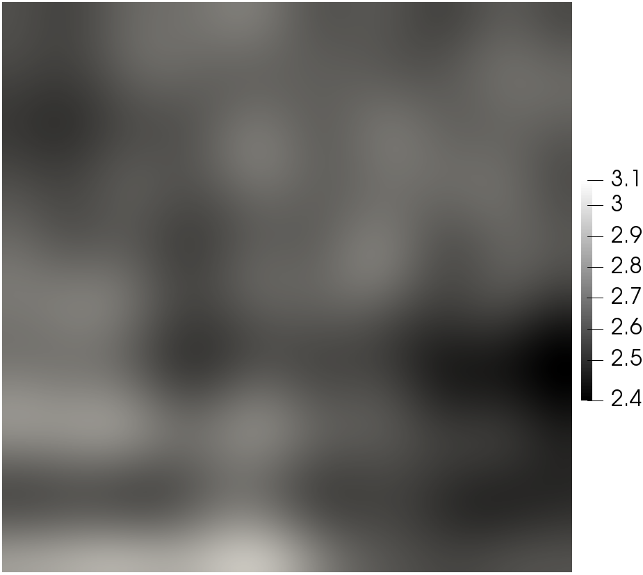
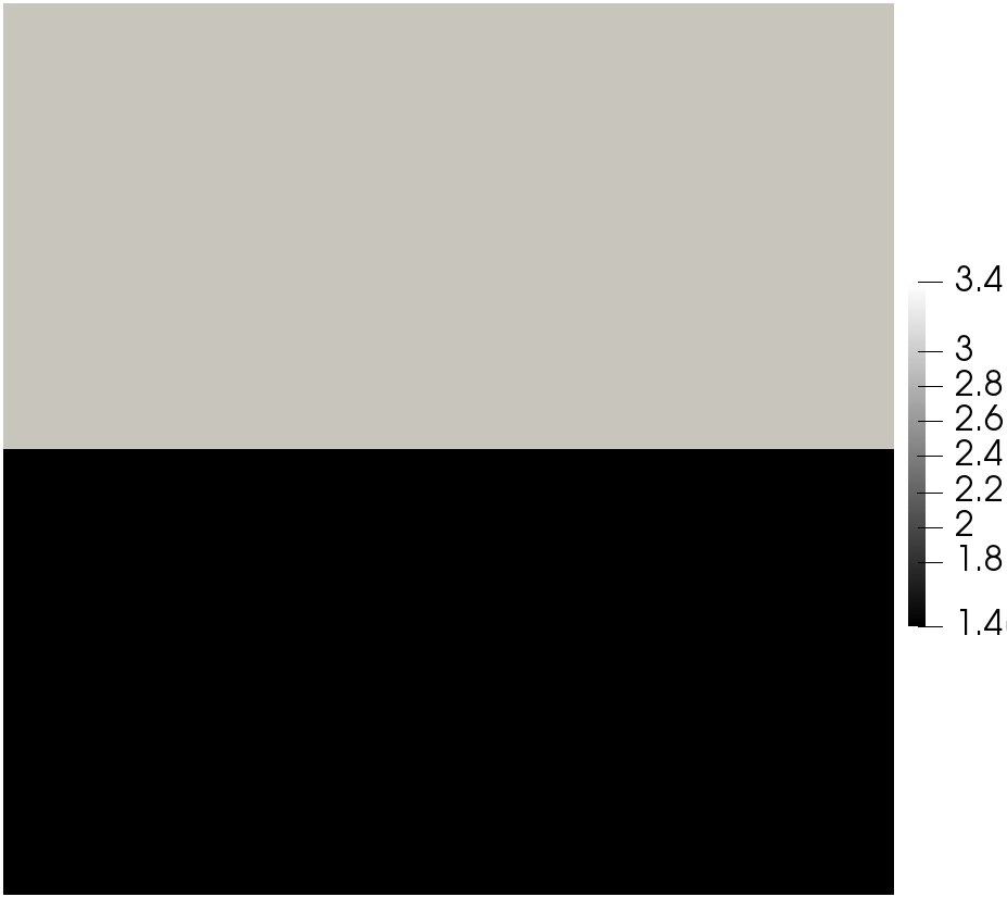
To demonstrate the effect of the random field choice on the convergence, we observe three different random fields. Example realizations of the fields are shown in Figure 1. We recall that for a random field $a$, the Karhunen–Loève expansion takes the form

$$a(x,\omega)=a_{0}+\sum_{i=1}^{\infty}\sqrt{\lambda_{i}}\phi_{i}(x)\xi_{i}(\omega),$$ (5.3)

where $\xi_{i}$ is a random variable with given probability distribution, and $\lambda_{i}$ and $\phi_{i}$ denote the eigenvalues and eigenfunctions associated with the compact self-adjoint operator defined via the covariance function $C\in L^{2}(D\times D)$ by

$$\mathcal{C}(\phi)(x)=\int_{D}C(x,y)\phi(y)\mathop{}\!\mathrm{d}y,\quad x\in D.$$

For simulations, we use a finite dimensional noise assumption to replace (5.3) with

$$a(x,\xi)=a_{0}+\sum_{i=1}^{m}\sqrt{\lambda_{i}}\phi_{i}(x)\xi_{i}(\omega).$$ (5.4)

For an interval $[a,b]$ where $a<b$, we denote the uniform distribution by $U(a,b)$ and the truncated normal distribution with parameters $\mu$ and $\sigma$ by $\mathcal{N}(\mu,\sigma,a,b)$

Remark 5.1.

Of course, truncating the Karhunen–Loève expansion after $m$ summands will introduce an additional error, in general. This can be included in the error estimates in Lemma 4.6 analogous to the error in the uncertain coefficient due to interpolation.

Example 1

For the first example (cf., [24, Example 9.37]), we choose $a_{0}=5,m=20$, and $\xi_{i}\sim U(-\sqrt{3},\sqrt{3})$ for $i=1,\dots,m$. The eigenfunctions and eigenvalues are given by

$$\tilde{\phi}_{j,k}(x):=2\cos(j\pi x_{2})\cos(k\pi x_{1}),\quad\tilde{\lambda}_{k,j}:=\frac{1}{4}\exp(-\pi(j^{2}+k^{2})l^{2}),\quad j,k\geq 1,$$

where we reorder terms so that the eigenvalues appear in descending order (i.e., $\phi_{1}=\tilde{\phi}_{1,1}$ and $\lambda_{1}=\tilde{\lambda}_{1,1}$) and we choose the correlation length $l=0.5$.

Example 2

For the second example, we generate a log-normal random field with truncated Gaussian noise by first generating a truncated expansion for a Gaussian field with a separable exponential, i.e., the covariance function has the form

$$C(x,y)=e^{-|x_{1}-y_{1}|/l_{1}-|x_{2}-y_{2}|/l_{2}}$$

on $D=[-\tfrac{1}{2},\tfrac{1}{2}]^{2}.$ The eigenfunctions are given by $\phi_{j}(x)=\phi_{i,1}(x_{1})\phi_{k,2}(x_{2})$ and the eigenvalues are $\lambda_{j}=\lambda_{i,1}\lambda_{k,2}$, where $\phi_{i,m},\lambda_{i,m}$ are for $m=1,2$ solutions to

$$\int_{-1/2}^{1/2}e^{-|x_{m}-y_{m}|/l_{m}}\phi^{m}(y_{m})\mathop{}\!\mathrm{d}y_{m}=\lambda^{m}\phi^{m}(x_{m}),\quad x_{m}\in[-\tfrac{1}{2},\tfrac{1}{2}].$$ (5.5)

Solutions to (5.5) have the analytic expression (cf., [24, Example 7.55])

$$\phi^{i,m} =\begin{cases}\sqrt{1/2+\sin(\omega_{i})/(2\omega_{i})}^{-1}\cos(\omega_{i}x_{m}),&i\text{ odd}\\ \sqrt{1/2-\sin(\omega_{i})/(2\omega_{i})}^{-1}\sin(\omega_{i}x_{m}),&i\text{ even}\end{cases}$$ (5.6)

$$\lambda_{i,m} =\frac{2l_{m}^{-1}}{\omega_{i}^{2}+l_{m}^{-2}},\quad\quad\quad\omega_{i}=\begin{cases}\hat{\omega}_{\lceil{i/2}\rceil},&i\text{ odd}\\ \tilde{\omega}_{i/2},&i\text{ even}\end{cases},$$

where $\hat{\omega}_{j}$ is the $j^{\text{th}}$ positive root of $l^{-1}-\omega\tan(\omega/2)$ and $\tilde{\omega}_{j}$ is the $j^{\text{th}}$ positive root of $l^{-1}\tan(\omega/2)+\omega.$ Sorting terms in (5.6) by decreasing eigenvalues and reindexing, we define the log-normal field with truncated Gaussian noise by

$$a(x,\xi)=e^{a_{0}+\sum_{i=1}^{m}\sqrt{\lambda_{i}}\phi_{i}(x)\xi_{i}(\omega)}$$ (5.7)

with $a_{0}=1$, $l_{1}=l_{2}=1$, $m=100$, and $\xi_{i}\sim\mathcal{N}(0,0.1,-100,100).$ In simulations, the random fields are additionally transformed to $(0,1)\times(0,1)$. For this choice, the trajectories of $a$ belong to $C^{t}(\bar{D})$ for all $t<1/2$; see [9, Lemma 2.3].

Example 3

We observe an example that does not satisfy Assumption 4.1. We partition $D$ into two non-overlapping subdomains $D_{1}$, $D_{2}$ and define a piecewise constant field by

$$a(x,\omega)=\xi_{1}(\omega)\mathds{1}_{D_{1}}(x)+\xi_{2}(\omega)\mathds{1}_{D_{2}}(x)$$ (5.8)

where $\mathds{1}_{D_{i}}$ is the indicator function of the set $D_{i}\subset D$ and $\xi_{i}$ are bounded, positive and independent random variables. In simulations, we let $D_{1}=(0,1)\times(1/2,1)$ and $D_{2}=(0,1)\times(0,1/2)$; we let $\xi_{1}\sim U(3,4)$ and $\xi_{2}\sim U(1,2)$.

(a) Example 1

(b) Example 2

(c) Example 3

Figure 1: Single realizations of each random field.

5.2 Experiments

Simulations were run on FEniCS [4] on a laptop with Intel Core i7 Processor (8 x 2.6 GHz) with 16 GB RAM. In all experiments, the initial mesh contained eight triangles and was uniformly refined using newest vertex bisection.

Effect of mesh refinement on objective function value

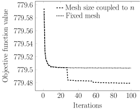
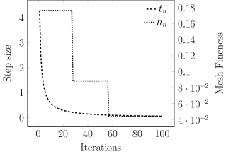
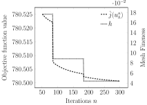
In the first experiment, we observe objective function values with and without mesh refinement for the random field in example 1. The strongly convex case is observed with $\lambda=0.1.$ A total of 1000 samples is taken at iteration $n=100$ and objective function values are compared. We use step sizes (4.12) where $\theta=1/(2\lambda)+1$, $\nu=2\theta K/(2\lambda\theta-1)-1$ and $K=5$. Without refinement, where the mesh is constant $h\approx 0.18$, $\hat{j}_{100}\approx 779.503$. With refinement, where the mesh is refined according to (4.12), we get $h_{100}\approx 0.04$ and $\hat{j}_{100}\approx 779.479$. Figure 2 shows clear jumps where the mesh is refined.

(a) Objective function

(b) Step size and mesh fineness

Figure 2: Behavior of objective function with and without mesh refinement.

Convergence plots - Strongly Convex Case

To demonstrate Algorithm 2 using (4.12), we choose the example for the strongly convex case with $\lambda=0.2$, $\theta>1/(2\lambda)+1$, $K=1$, and $\nu=2\theta K/(2\lambda\theta-1)-1$, and finally, $c=17.5$, which was chosen to prevent the mesh from refining too aggressively. To generate reference solutions, the algorithm was run for $n=3000$ iterations with $h_{1000}\approx 0.0044$ to get $\bar{u}:=u_{3000}$; these solutions are shown for each of the random fields in Figure 3.

(a) Example 1

(b) Example 2

(c) Example 3

Figure 3: Reference solutions for strongly convex case.

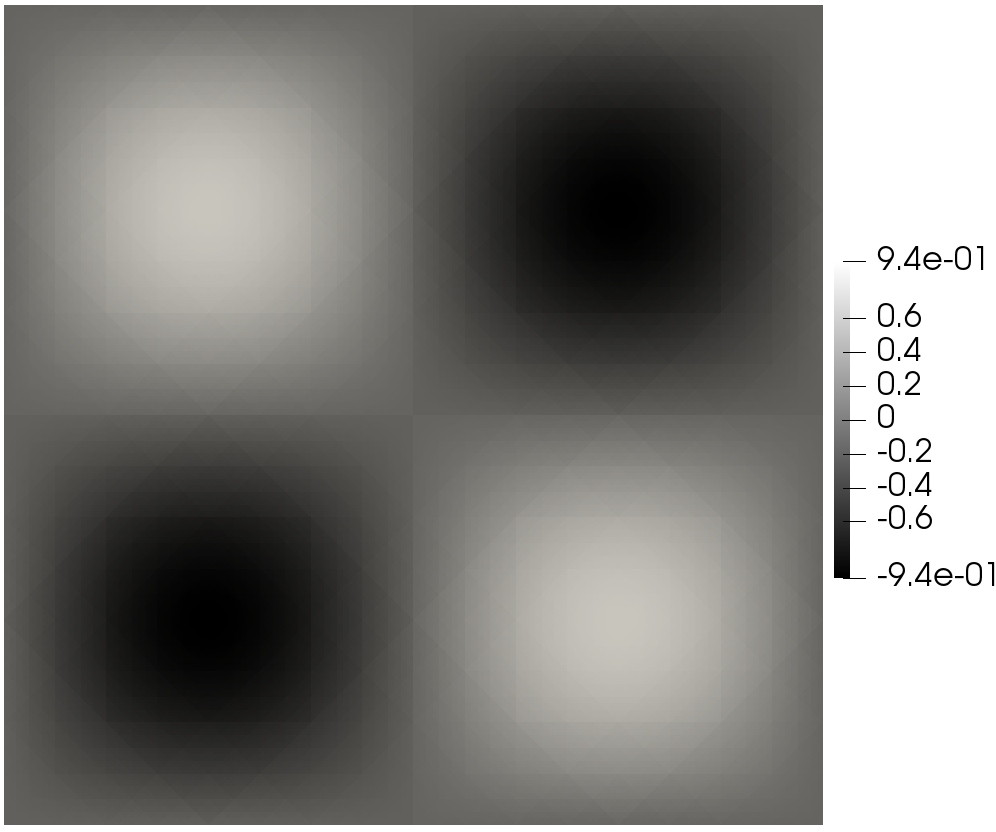
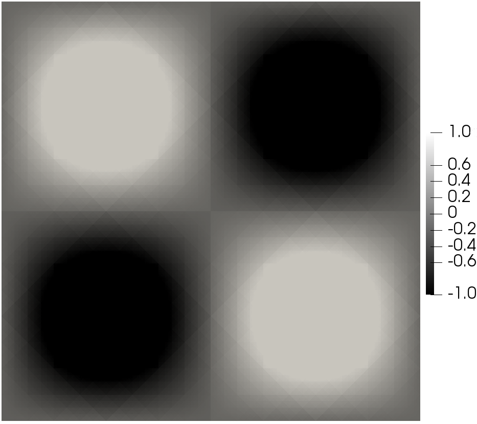
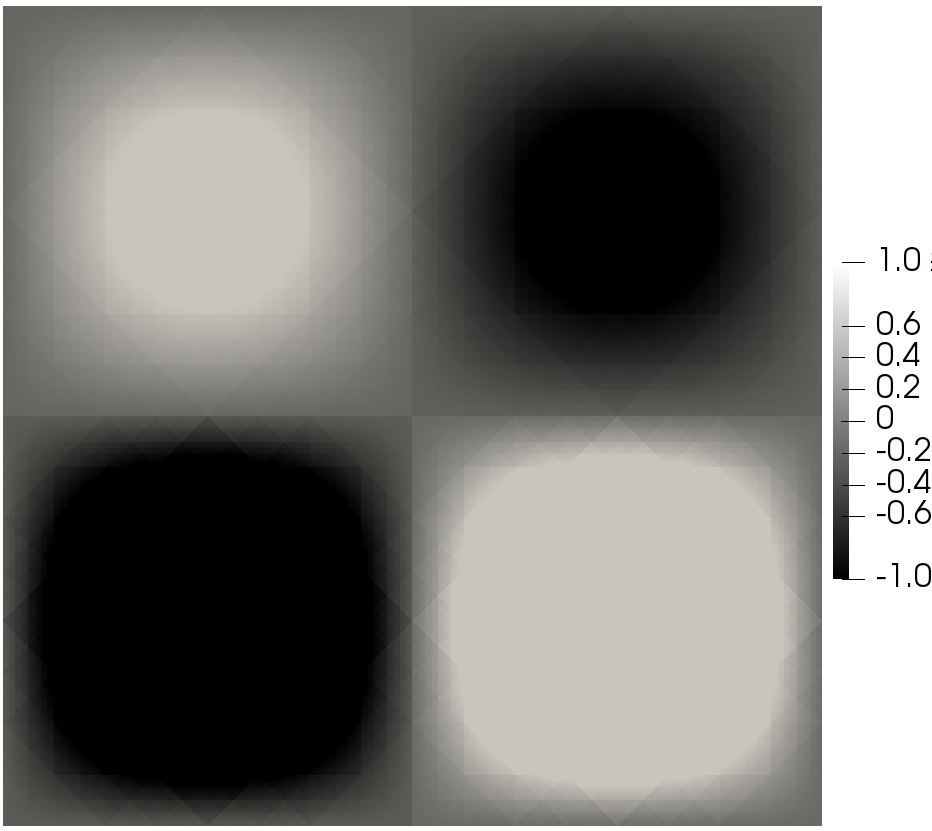
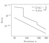
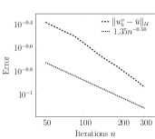
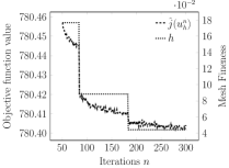
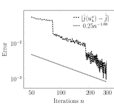
We observe behavior of the algorithm for a single run with $300$ iterations. To approximate objective function values, $m=1000$ samples are generated to get $\hat{j}(u_{h}^{n})=\tfrac{1}{m}\sum_{i=1}^{m}J(u_{h}^{n},\xi^{n,i})$, where $\xi^{n,i}$ denotes a newly generated $i^{\text{th}}$ sample at iteration $n$. We set $\hat{\bar{j}}:=\hat{j}(u_{h}^{3000}).$ We observe objective function decay and convergence rates $\lVert u_{h}^{n}-\bar{u}\rVert_{\mathcal{U}}$ and $|\hat{j}(u_{h}^{n})-\hat{\bar{j}}|$ for a single run of the algorithm for each of the random fields; see Figure 4–6. To approximate $\lVert u_{h}^{n}-\bar{u}\rVert_{\mathcal{U}}$, we project $u_{h}^{n}$ onto the fine mesh used for $\bar{u}$ and compute the error on the fine mesh. In each example, we see clear jumps in the objective function value when the mesh is refined, followed by decay at or better than the expected rate. A single run of 1000 iterations with mesh refinement took 36% of the CPU time when compared to computations on a fixed mesh (corresponding to $h_{1000}\approx 0.011$).

(a) Objective function

(b) Error in iterates

(c) Error in objective function

Figure 4: Strongly convex functional with smooth random field (example 1).

(a) Objective function

(b) Error in iterates

(c) Error in objective function

Figure 5: Strongly convex functional with log-normal random field (example 2).

(a) Objective function

(b) Error in iterates

(c) Error in objective function

Figure 6: Strongly convex functional with piecewise constant random field (example 3).

Convergence Plots - Averaging

For the general convex case, we choose the convex example with the modified constraint (5.1). We denote the discretization of the average of iterates $i$ to $N$ $\tilde{u}_{i}^{N}$, defined in (3.12), as $\tilde{u}_{i,h}^{N}.$ We note that the bound on the second moment of the stochastic gradient $M$ can be analytically computed as in [13] by $M=\lVert G(u,\xi)\rVert_{\mathcal{U}}^{2}\leq[C(\lVert y^{D}\rVert_{\mathcal{U}}+C(\lVert u\rVert_{\mathcal{U}}+\lVert e^{D}\rVert_{\mathcal{U}}))]^{2}$ with $C=C_{p}^{2}/a_{\min}$, where $C_{p}$ is the Poincaré constant, which can be bounded by $\text{diam}(D)/\pi=\sqrt{2}/\pi$ [29]. Note that $\lVert y^{D}\rVert_{\mathcal{U}}^{2}=5/2$, $\lVert e^{D}\rVert_{\mathcal{U}}^{2}=1+9\pi^{4}$ and $\lVert u\rVert_{\mathcal{U}}\leq 1$ for all $u\in\mathcal{U}$. In addition, for example 1, $a_{\min}\approx 3.55$; for example 2, $a_{\min}\approx 2.72$; for example 3, $a_{\min}=1$.

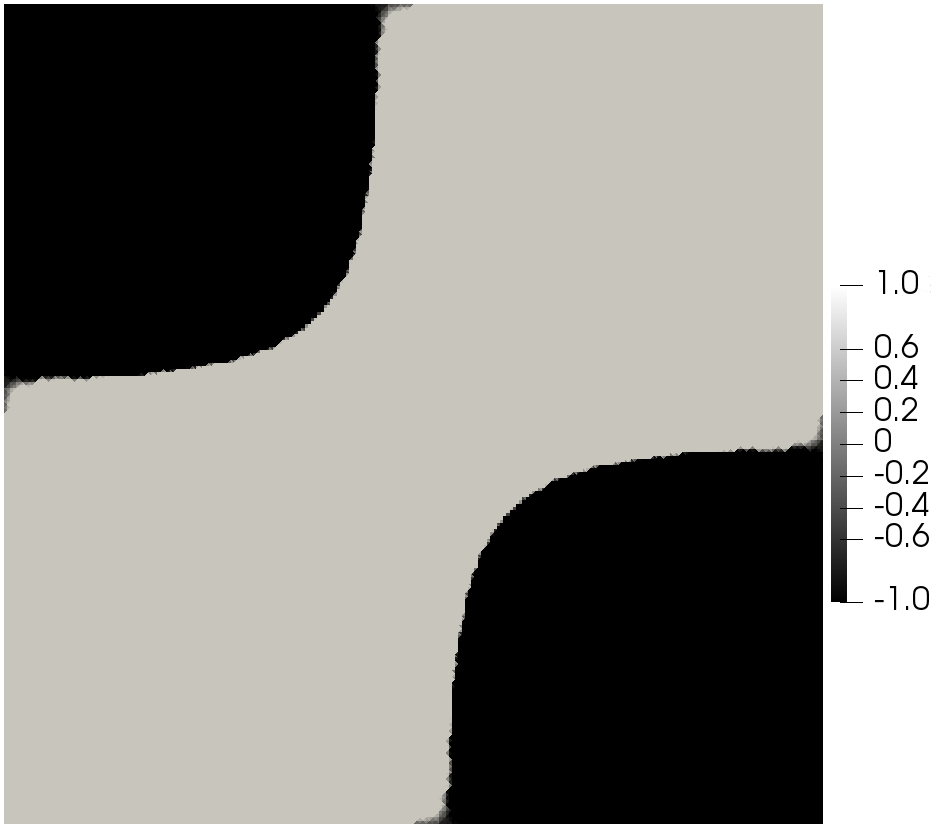
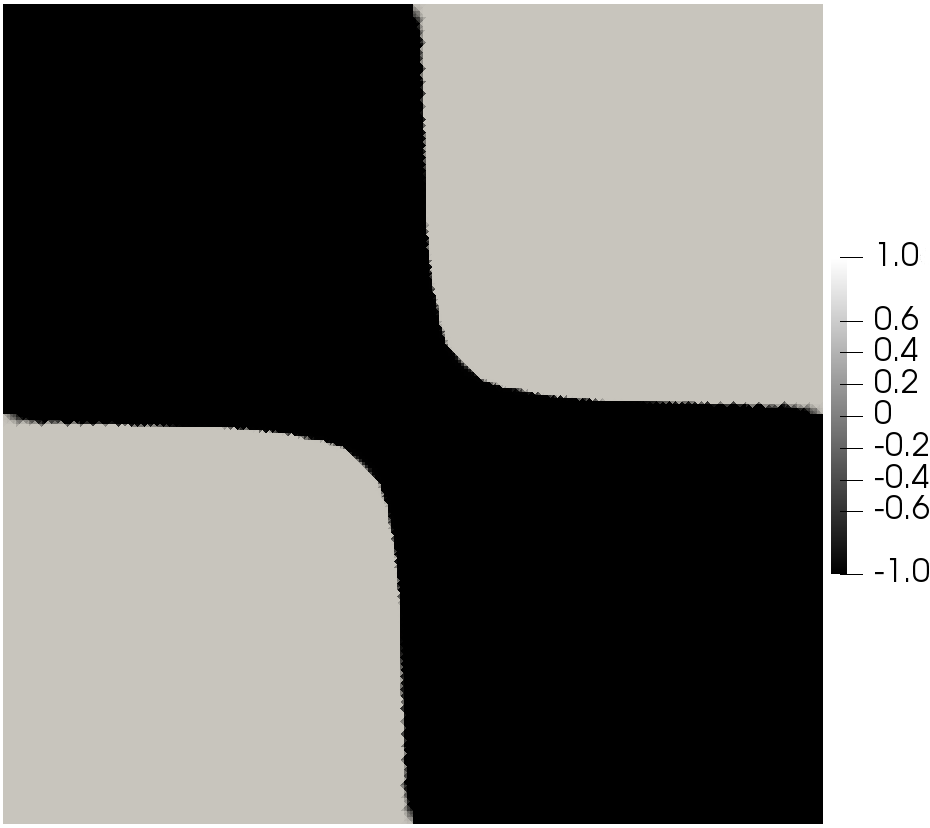
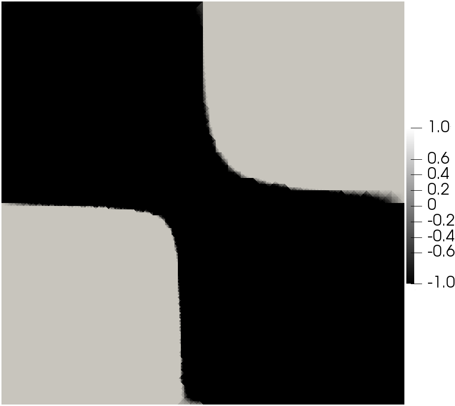
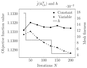
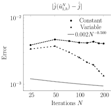
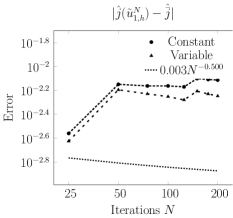
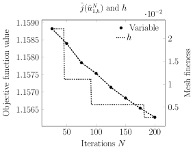
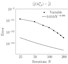
To generate reference solutions, the algorithm is run with the variable step size rule (4.16) with $\theta=50$ for $n=5000$ iterations with $h_{5000}\approx 0.0055$ and $\alpha=0.1$ for the averaging factor to get $\bar{u}=\tilde{u}_{4500,h}^{5000}$; see Figure 7 for the solutions for each random field. To approximate objective function values, $m=5000$ samples were generated to get $\hat{j}(\tilde{u}_{\lceil\alpha N\rceil,h}^{N})=\tfrac{1}{m}\sum_{i=1}^{m}J(\tilde{u}_{\lceil\alpha N\rceil,h}^{N},\xi^{n,i})$, where $\xi^{n,i}$ denotes a newly generated $i^{\text{th}}$ sample at iteration $n$. We set $\hat{\bar{j}}:=\hat{j}(\bar{u})$ and use $\alpha=0.5$ for the experiments. We choose a fixed number of iterations $N\in\{25,50,\dots,250\}$ and for each of these iteration numbers, we ran a separate simulation using the step sizes and mesh refinement rules informed by (4.14) and (4.16). To prevent the mesh from refining too quickly, we choose $c=2$. For the variable step size rule (4.16) we use $\theta=1.$ Plots of convergence for example 1 and example 2 are shown in Figure 8–Figure 9. Again we see agreement with the theory, with clear jumps when the mesh is refined, both with constant and variable step sizes. We also note that positive jumps in the objective function value are possible when the mesh is refined, as seen in Figure 9–Figure 10. For the third example, we modified the random field so that we can view the effect of reduced regularity more clearly; we used $\xi\sim U(5,5.1)$ and $U(1,1.1)$. In Figure 10–Figure 10, we see a decrease in convergence rate, which could be caused by missing regularity due to the jump discontinuity in the random field as mentioned in Remark 4.8. We reran the experiment with the guess $\min(2s,t,1)=0.5$, which results in a more aggressive mesh refinement and convergence according to the theory; see Figure 11. In all examples, the variable step size yields a lower error for the same number of iterations when compared to the constant step size rule.

(a) Example 1

(b) Example 2

(c) Example 3

Figure 7: Reference solutions for general convex case.

(a) Objective function and mesh fineness

(b) Error in objective function

Figure 8: General convex functional with smooth random field (example 1) using constant and variable step size rules.

(a) Objective function and mesh fineness

(b) Error in objective function

Figure 9: General convex functional with log-normal random field (example 2) using constant and variable step size rules.

(a) Objective function and mesh fineness

(b) Error in objective function

Figure 10: General convex functional with piecewise constant random field (example 3) using constant and variable step size rules.

(a) Objective function and mesh fineness

(b) Error in objective function

Figure 11: General convex functional with piecewise constant random field (example 3) and $\min(2s,t,1)=0.5$ using variable step size rules.

6 Conclusion

In this paper, we developed efficiency estimates incorporating numerical error for the projected stochastic gradient algorithm applied to stochastic optimization problems in Hilbert spaces. We distinguish between a strongly convex functional and a general convex case, where in the latter case we use averaging to allow for larger step sizes. These estimates informed how to balance the error and step size rules for both the strongly convex case and the convex case with averaging. We introduced a model stochastic optimization problem with a PDE constraint subject to uncertain coefficients. Using a priori error estimates for the PDE constraint, we developed a mesh refinement strategy that, coupled with reducing step sizes, yields convergence rates according to our efficiency estimates. This was demonstrated using three different random fields on problems with and without a regularization term, which allowed us to test our convergence theory on a strongly convex and general convex objective function.

References

- [1] R. A. Adams and J. J. Fournier, Sobolev Spaces, Elsevier, 2003, \urlhttps://doi.org/10.1016/S0079-8169(03)80002-8.
- [2] A. Alexanderian, N. Petra, G. Stadler, and O. Ghattas, Mean-variance risk-averse optimal control of systems governed by PDEs with random parameter fields using quadratic approximations, SIAM/ASA J. Uncertain. Quantif., 5 (2017), pp. 1166–1192, \urlhttps://doi.org/10.1137/16m106306x.
- [3] A. A. Ali, E. Ullmann, and M. Hinze, Multilevel Monte Carlo analysis for optimal control of elliptic PDEs with random coefficients, SIAM/ASA J. Uncertain. Quantif., 5 (2017), pp. 466–492, \urlhttps://doi.org/10.1137/16M109870X.
- [4] M. S. Alnæs, J. Blechta, J. Hake, A. Johansson, B. Kehlet, A. Logg, C. Richardson, J. Ring, M. E. Rognes, and G. N. Wells, The FEniCS project version 1.5, Arch. of Numerical Software, 3 (2015), \urlhttps://doi.org/10.11588/ans.2015.100.20553.
- [5] I. Babuška, F. Nobile, and R. Tempone, A stochastic collocation method for elliptic partial differential equations with random input data, SIAM J. Numer. Anal., 45 (2007), pp. 1005–1034, \urlhttps://doi.org/10.1137/050645142.
- [6] I. Babuška, R. Tempone, and G. E. Zouraris, Galerkin finite element approximations of stochastic elliptic partial differential equations, SIAM J. Numer. Anal., 42 (2004), pp. 800–825, \urlhttps://doi.org/10.1137/s0036142902418680.
- [7] A. Borzì and G. Von Winckel, Multigrid methods and sparse-grid collocation techniques for parabolic optimal control problems with random coefficients, SIAM J. Sci. Comput., 31 (2009), pp. 2172–2192, \urlhttps://doi.org/10.1137/070711311.
- [8] S. C. Brenner and L. R. Scott, The Mathematical Theory of Finite Element Methods, Springer Verlag, New York, 3. ed., 2008, \urlhttps://doi.org/10.1007/978-0-387-75934-0.
- [9] J. Charrier, R. Scheichl, and A. L. Teckentrup, Finite element error analysis of elliptic PDEs with random coefficients and its application to multilevel Monte Carlo methods, SIAM J. Numer. Anal., 51 (2013), pp. 322–352, \urlhttps://doi.org/10.1137/110853054.
- [10] P. Chen, U. Villa, and O. Ghattas, Taylor approximation and variance reduction for PDE-constrained optimal control under uncertainty, J. Comput. Phys., 385 (2019), pp. 163–186, \urlhttps://doi.org/10.1016/j.jcp.2019.01.047.
- [11] P. G. Ciarlet, The Finite Element Method for Elliptic Problems, vol. 4 of Studies in Mathematics and Applications, North-Holland, 1978, \urlhttps://doi.org/10.1137/1.9780898719208.
- [12] S. Garreis and M. Ulbrich, A fully adaptive method for the optimal control of semilinear elliptic PDEs under uncertainty using low-rank tensors, Preprint, Technical University of Munich, (2019+).
- [13] C. Geiersbach and G. Pflug, Projected stochastic gradients for convex constrained problems in Hilbert spaces, SIAM J. Optim., 29 (2019), pp. 2079–2099, \urlhttps://doi.org/10.1137/18m1200208.
- [14] P. Grisvard, Elliptic Problems in Nonsmooth Domains, Monographs and studies in Mathematics, Pitman, Boston, 1. ed., 1985, \urlhttps://doi.org/10.1137/1.9781611972030.
- [15] M. Gunzburger, C. Webster, and G. Zhang, Stochastic finite element methods for partial differential equations with random input data, Acta Numer., 23 (2014), pp. 521–650, \urlhttps://doi.org/10.1017/s0962492914000075.
- [16] P. A. Guth, V. Kaarnioja, F. Y. Kuo, C. Schillings, and I. H. Sloan, A quasi-Monte Carlo method for an optimal control problem under uncertainty, arXiv preprint arXiv:1910.10022, (2019).
- [17] E. Haber, M. Chung, and F. Herrmann, An effective method for parameter estimation with PDE constraints with multiple right-hand sides, SIAM J. Optim., 22 (2012), \urlhttps://doi.org/10.1137/11081126x.
- [18] R. Haller-Dintelmann, H. Meinlschmidt, and W. Wollner, Higher regularity for solutions to elliptic systems in divergence form subject to mixed boundary conditions, Ann. Mat. Pura Appl., 198 (2019), pp. 1227–1241, \urlhttps://doi.org/10.1007/s10231-018-0818-9.
- [19] L. Hou, J. Lee, and H. Manouzi, Finite element approximations of stochastic optimal control problems constrained by stochastic elliptic PDEs, J. Math. Anal. Appl., 384 (2011), pp. 87–103, \urlhttps://doi.org/10.1016/j.jmaa.2010.07.036.
- [20] J. Kiefer and J. Wolfowitz, Stochastic estimation of the maximum of a regression function, Ann. Math. Statistics, 23 (1952), pp. 462–466, \urlhttps://doi.org/10.1214/aoms/1177729392.
- [21] D. Kouri, M. Heinkenschloss, D. Ridzal, and B. G. V. B. Waanders, A trust-region algorithm with adaptive stochastic collocation for PDE optimization under uncertainty, SIAM J. Sci. Comput., 35 (2013), pp. A1847–A1879, \urlhttps://doi.org/10.1137/120892362.
- [22] D. Kouri, M. Heinkenschloss, D. Ridzal, and B. V. B. Waanders, Inexact objective function evaluations in a trust-region algorithm for PDE-constrained optimization under uncertainty, SIAM J. Sci. Comput., 36 (2014), \urlhttps://doi.org/10.1137/140955665.
- [23] D. P. Kroese, T. Taimre, and Z. I. Botev, Handbook of Monte Carlo methods, vol. 706, John Wiley & Sons, 2011, \urlhttps://doi.org/10.1002/9781118014967.
- [24] G. Lord, C. Powell, and T. Shardlow, An Introduction to Computational Stochastic PDEs, Cambridge University Press, 2014, \urlhttps://doi.org/10.1017/cbo9781139017329.008.
- [25] A. Lunardi, Interpolation Theory, Edizioni della Normale, Pisa, 20018, \urlhttps://doi.org/10.1007/978-88-7642-638-4.
- [26] M. Martin, S. Krumscheid, and F. Nobile, Analysis of stochastic gradient methods for PDE-constrained optimal control problems with uncertain parameters, tech. report, École Polytechnique MATHICSE Institute of Mathematics, 2018.
- [27] C. Meyer, A. Rademacher, and W. Wollner, Adaptive optimal control of the obstacle problem, SIAM J. Sci. Comput., 37 (2015), pp. A918–A945, \urlhttps://doi.org/10.1137/140975863.
- [28] A. Nemirovski, A. Juditsky, G. Lan, and A. Shapiro, Robust stochastic approximation approach to stochastic programming, SIAM J. Optim., 19 (2009), pp. 1574–1609, \urlhttps://doi.org/10.1137/070704277.
- [29] L. Payne and H. Weinberger, An optimal Poincaré inequality for convex domains, Arch. Rational Mech. Anal., 5 (1960), pp. 286–292, \urlhttps://doi.org/10.1007/bf00252910.
- [30] R. Rannacher and B. Vexler, Adaptive finite element discretization in PDE-based optimization, GAMM-Mitt, 33 (2010), pp. 177–193, \urlhttps://doi.org/10.1002/gamm.201010014.
- [31] R. Rannacher, B. Vexler, and W. Wollner, A posteriori error estimation in PDE-constrained optimization with pointwise inequality constraints, in Constrained Optimization and Optimal Control for Partial Differential Equations, vol. 160 of International Series of Numerical Mathematics, Springer, 2012, pp. 349–373, \urlhttps://doi.org/10.1007/978-3-0348-0133-1_19.
- [32] H. Robbins and S. Monro, A stochastic approximation method, Ann. Math. Statist., 22 (1951), pp. 400–407, \urlhttps://doi.org/10.1214/aoms/1177729586.
- [33] E. Rosseel and G. Wells, Optimal control with stochastic PDE constraints and uncertain controls, Comput. Methods Appl. Mech. Engrg., (2012), pp. 152–167, \urlhttps://doi.org/10.1016/j.cma.2011.11.026.
- [34] C. Schwab and C. J. Gittelson, Sparse tensor discretizations of high-dimensional parametric and stochastic PDEs, Acta Numer., 20 (2011), pp. 291–467, \urlhttps://doi.org/10.1017/s0962492911000055.
- [35] H. Tiesler, R. M. Kirby, D. Xiu, and T. Preusser, Stochastic collocation for optimal control problems with stochastic PDE constraints, SIAM J. Control Optim., 50 (2012), pp. 2659–2682, \urlhttps://doi.org/10.1137/110835438.
- [36] H. Triebel, Interpolation Theory, Function Spaces, Differential Operators, Johann Ambrosius Barth Verlag; Heidelberg, Leipzig, 2., rev. and enl. ed., 1995.
- [37] E. Ullmann, H. C. Elman, and O. G. Ernst, Efficient iterative solvers for stochastic Galerkin discretizations of log-transformed random diffusion problems, SIAM J. Sci. Comput., 34 (2012), pp. A659–A682, \urlhttps://doi.org/10.1137/110836675.