The S-matrix Bootstrap IV:
Multiple Amplitudes
Alexandre Homrich, João Penedones, Jonathan Toledo, Balt C. van Rees, Pedro Vieira ††#@gmail.com&/@{alexandre.homrich,jpenedones,jonathan.campbell.toledo,baltvanrees,pedrogvieira}
Perimeter Institute for Theoretical Physics,
Waterloo, Ontario N2L 2Y5, Canada
ICTP South American Institute for Fundamental Research, IFT-UNESP, São Paulo, SP Brazil 01440-070
Fields and Strings Laboratory,
Institute of Physics, École Polytechnique Fédérale de Lausanne (EPFL),
CH-1015 Lausanne,
Switzerland
Centre for Particle Theory, Department of Mathematical Sciences, Durham University, Lower Mountjoy, Stockton Road, Durham, England, DH1 3LE
Abstract
We explore the space of consistent three-particle couplings in -symmetric two-dimensional QFTs using two first-principles approaches. Our first approach relies solely on unitarity, analyticity and crossing symmetry of the two-to-two scattering amplitudes and extends the techniques of [2] to a multi-amplitude setup. Our second approach is based on placing QFTs in AdS to get upper bounds on couplings with the numerical conformal bootstrap, and is a multi-correlator version of [1]. The space of allowed couplings that we carve out is rich in features, some of which we can link to amplitudes in integrable theories with a symmetry, e.g., the three-state Potts and tricritical Ising field theories. Along a specific line our maximal coupling agrees with that of a new exact S-matrix that corresponds to an elliptic deformation of the supersymmetric Sine-Gordon model which preserves unitarity and solves the Yang-Baxter equation.
1 Introduction
The bootstrap of the two-to-two S-matrix of the lightest particle in a relativistic unitarity quantum field theory was recently revived in [1, 2, 3] and extended to particles with flavour in [7, 8, 9, 10]. These works can be seen as gapped counterparts of the conformal bootstrap explorations in [4, 5] and [11] (without and with flavour respectively). Here we initiate the bootstrap analysis of S-matrix elements involving different external particles in symmetric theories. This multiple amplitude study again mimics a similar recent development in the conformal bootstrap, namely the multiple correlator analysis of the Ising model which famously gave rise to the CFT islands in [12].111While walking hand in hand as illustrated in the previous paragraph, the S-matrix and the conformal bootstrap also have significant differences. In the CFT bootstrap we exclude theories; once excluded, a theory can never be accepted; with better computers we exclude more. In the S-matrix bootstrap of [2, 3] we include theories; by constructing explicit solutions to crossing and unitarity some parameters are shown to be allowed; with better computers we include more. (In the S-matrix bootstrap when we impose new physical conditions we will exclude some of the previously found S-matrices though so the process is not as monotonic as in the CFT bootstrap.) The two bootstraps are thus two faces of a same coin, the Yin and the Yang, the darkness and the light, the chaos and the order. For a recent review of the conformal bootstrap state of the art see [13].
We will consider two-dimensional QFTs with exactly two stable particles of masses and . We will assume the theory to be parity and time-reversal invariant and both particles to be parity even. For simplicity we will also postulate the existence of a symmetry, under which the first particle is odd and the second particle is even.222In two dimensions theories with fermions and scalars are naturally symmetric theories so the setup here applies as well to any theories with scalars and fermions, not necessarily supersymmetric. This means that the nonzero three-particle couplings are and , which can be defined non-perturbatively in terms of the residues of a pole in a suitable S-matrix element. In the first part of this paper we will analyze all the two-to-two S-matrices of particles 1 and 2 and use crossing symmetry, analyticity and unitarity to explore the space of possible points in the (non-dimensionalized) plane as a function of – see figure 8 on page 8 to get an idea. In order to avoid singularities or Coleman-Thun poles [6], which complicate the analytic structure of the scattering amplitudes, we will restrict ourselves to
| (1) |
Note that we allow also.
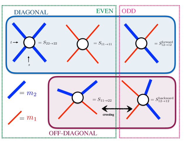
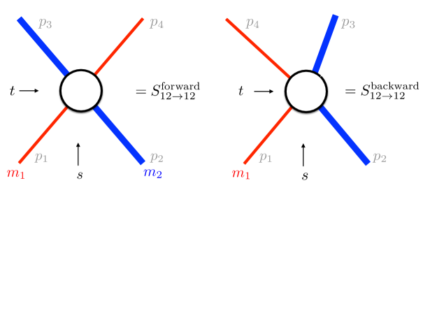
Under the stated assumptions there are five different physical two-to-two scattering processes as shown in figure 1. These can be grouped either according to the nature of their intermediate states, which can be odd or even, or according to whether they are ‘diagonal’ or not. To wit, for a diagonal process the incoming and outgoing momenta are the same whereas for an off-diagonal process they are different.333As explained further below, in two dimensions the scattering angle can take only two values by kinematical restrictions; the outgoing momenta are essentially ‘locked’ in terms of the incoming momenta. Unlike in higher dimensions, there is therefore no (analytic) function interpolating between forward and backward scattering. As is also indicated in figure 1, we call the diagonal process ‘forward’ scattering, and the off-diagonal process ‘backward’.
In section 2 we will state in detail the conditions of unitarity, analyticity, and crossing symmetry that these five processes must obey. To guide ideas let us mention two conspicuous facts. First, we note that crossing symmetry flips the and axes on the diagram. This relates the two off-diagonal processes and thereby reduces the number of independent amplitudes (i.e. functions of the Mandelstam invariant) to four. Of course, it also imposes a non-trivial constraint on the amplitudes for the diagonal processes. Second, we observe that particle 1 can appear as an intermediate state in all the odd processes and gives rise to a pole in these amplitudes with residue proportional to , whereas particle 2 gives rise to poles in all the even amplitudes with residues proportional to , or , depending on the process. These poles can be thought of as our definition of the corresponding couplings.444The astute reader will have noticed that this defines the couplings only up to an overall sign flip, leading to an obvious reflection symmetry in some of our plots.
1.1 Quick comparison with single-correlator bounds
As a warm up exercise let us first discuss the three diagonal processes in isolation and explain how the methods discussed in [2, 3, 15, 16] already lead to some constraints on the couplings.
The analyticity and crossing symmetry of the diagonal processes in the Mandelstam plane is pretty straightforward. For example, the odd process has a two-particle -channel cut starting at and a pole at with residue proportional to , plus the crossed -channel singularities obtained by swapping . The even processes and have their two-particle -channel cuts starting at and a pole with residue or , again plus the crossed -channel singularities obtained by swapping or . As for unitarity, notice that the discontinuity across the cut is always positive, but it is bounded from above only for physical , which means for and for . Therefore only for the lightest of the two particles is the discontinuity everywhere bounded from above, whereas for the other particle the discontinuity can be arbitrarily large (but not negative) in the interval between and .
We can bound the couplings as follows. First let us bound by using the maximum modulus principle for following [2, 3, 15, 16]. We define
| (2) |
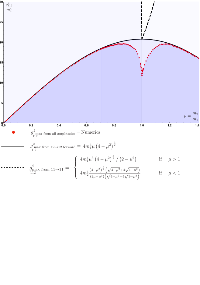
with . The function is free of singularities (since we divided out by functions with poles at the pole location of the amplitudes) and is bounded at the – and – channel cuts (since the functions we divided by are phases at those cuts and the amplitude is bounded). Therefore must have absolute value smaller or equal to everywhere, and in particular at and where we can simply read off the maximally allowed couplings in these amplitudes. This leads to a universal upper bound on , which is the solid line in figure 2.
The exact same analysis can be used for the elastic amplitude for the lightest of the two particles. If we denote this by , so , then the maximum modulus principle for
| (3) |
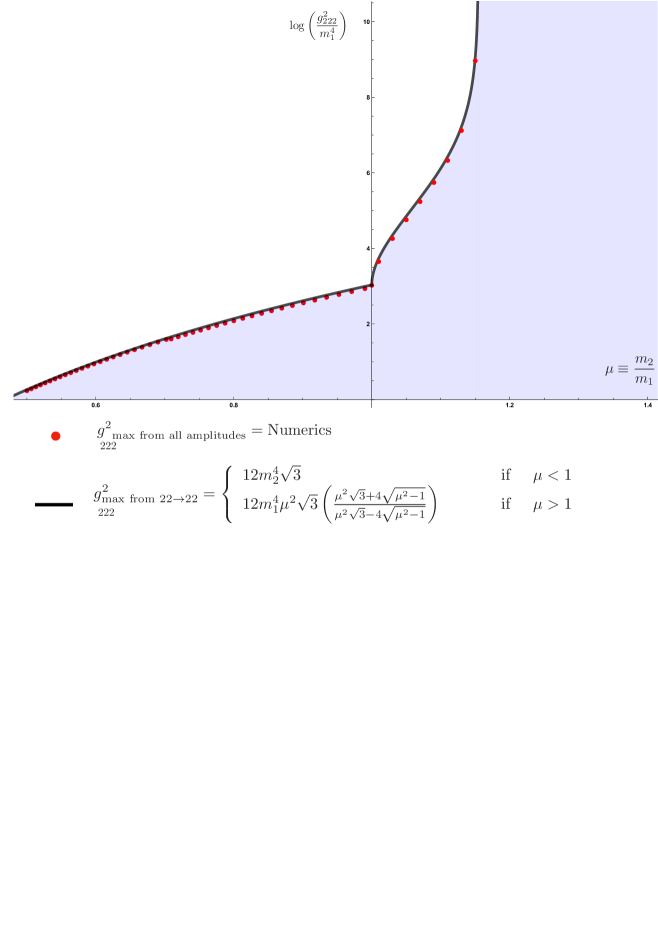
gives a bound on the coupling appearing on , which is . This is the dashed line for in figure 2 and the solid line for in figure 3.
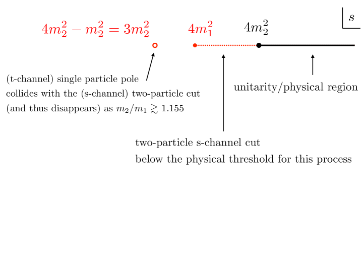
Finally we can use the techniques of [2] to also derive a bound on from the amplitude even when is not the lightest particle. In this case there is a cut which is not bounded directly by unitarity as depicted in figure 4. As we derive in appendix C, the amplitude with maximal is given by
| (4) |
The corresponding bound on is plotted as the solid line in figure 3 for . As the figure shows, the bound actually disappears for , which is due the t-channel pole colliding with the s-channel cut in the process at this mass ratio. This is the simplest instance of a phenomenon we call screening. It is detailed in figure 4 and we will encounter it again below. In the same way we could obtain a bound on from the process even when is the heaviest particle. This bound corresponds to the dashed line in figure 2 for , and is always less restrictive than the bound from .
This concludes our discussion of the single-amplitude results. As a preview for the more detailed numerical results presented below, we already marked in figures 2 and 3 in red dots our best numerical values of the coupling obtained from a simultaneous analysis of the full set of two-to-two amplitudes depicted in figure 1. Figure 2 displays a clear improvement over the quick single-amplitude analysis for , with an intriguing kink at . It would be fascinating to find if this kink corresponds to a physical theory. On the other hand, in figure 3 we see no improvement over the single-amplitude results. In fact, in section 3 we will prove that the maximal value of in the multi-amplitude analysis saturates the single-amplitude analytic bounds just derived. In the same section we will show a more complete picture by considering the entire plane.
1.2 QFT in AdS
As shown in [1], there exists a completely orthogonal approach towards the problem of determining the maximal couplings in QFT. Rather than working from the S-matrix, which required analyticity assumptions that in general dimension are not very well understood, the idea is to consider QFTs on an AdS background. The boundary correlators of such a QFT, which are defined in a similar way as in the AdS/CFT correspondence, behave much like conformal correlation functions in one lower dimension . By applying numerical conformal bootstrap methods of [4] one can put a universal upper bound on the three-point couplings of QFTs in AdS. One can then extrapolate this bound to the flat-space limit (by sending all scaling dimensions to infinity), resulting in putative bounds for flat-space QFTs. In [1, 2] this was shown to work extremely well for two-dimensional QFTs: a precise match was found between the single-correlator analysis using the conformal bootstrap, and the single-amplitude analysis that we partially reviewed above.
In this work we continue these explorations. As discussed further in section 4, the symmetric setup that we consider is easily translated to a multi-correlator conformal bootstrap problem for QFTs in AdS. In most cases we again find a very good match, and in particular we are able to recover the coupling of the 3-state Potts field theory from the conformal crossing equations. For large-ish mass ratios, however, we will see that the multi-correlator bootstrap appears to be less powerful than even the single-amplitude bootstrap.
1.3 Outline
The symmetric S-matrix bootstrap is fully spelled out in section 2 and analysed numerically in section 3 leading to various bounds on the allowed coupling space for various mass ratios as illustrated in figure 8. In section 3.3 we discuss integrable symmetric theories with and how some of them nicely show up at the boundary of the allowed S-matrix space found in the numerical bootstrap. These include a massive deformation of the -state Potts model, the super-symmetric Sine-Gordon model and a SUSY breaking integrable elliptic deformation of the super-symmetric Sine-Gordon which seems to be novel as far as we know. Section 4 contains the results from the QFT in AdS analysis. Various appendices complement the main text with further extensions. (For example, the special role of the Tricritical Ising model as a kink in the space of S-matrices is discussed in appendix H.)
2 Multiple amplitudes
2.1 Kinematics of the various preserving processes
There are six two-to-two processes involving particles (odd) and (even) in a two dimensional symmetric theory. We also assume time-reversal and parity symmetry. Four of those six are even processes where we scatter either or into either or . Of those four, two are trivially related by time-reversal,
| (5) |
so we can ignore one of them (say ) in what follows. The remaining two processes are odd processes where we scatter the odd particle against the even particle obtaining those same two particles in the future. As explained in the introduction this process splits into two possibilities which we call the forward and the backward component, see figures 1 and 5.
In two dimensions, any process depends uniquely on the center of mass energy or equivalently on the Mandelstam invariant
| (6) |
This in particular means that the other two Mandelstam invariants
| (7) |
are completely determined in terms of . It is important to find the precise relation because crossing symmetry permutes the three Mandelstam invariants and therefore leads to symmetries of the amplitudes that we need to impose. In a process555In the convention , , and . involving
| (8) |
The first equal sign is the two dimensional constraint: in two dimensions is always a linear combination of the two-vectors and and hence the determinant vanishes. In the second equal sign we used the on-shell conditions and momentum conservation. For example and so on. Evaluated explicitly and combined with the previous linear constraint on the Mandelstam invariants, this can be cast in a nice symmetric form:
| (9) |
where .
Let us now specialize to the preserving cases mentioned above. For the simplest processes corresponding to all equal masses (i.e. for and ) the condition dramatically simplifies into which leads to or or . In fact, we can not set since by definition we assume to be constructed from two incoming particles and setting or is the same up to a simple relabelling of the final particles which we can always do for indistinguishable particles. Hence without loss of generality we can set recovering the famous result that elastic scattering of identical particles in two dimensions has zero momentum transfer.
Next we have the processes involving two particles of mass and two particles of mass . Here it matters whether the two particles of the same mass are both incoming or if one is incoming and the other is outgoing. Let us start first with the second case so that we can set and in agreement with the conventions of figure 5. Then we obtain a nice factorization of the constraint (9) into
| (10) |
with two clear solutions: corresponding to forward scattering and corresponding to the more complicated backward scattering. Note that in forward scattering the final momenta are equal to the initial momenta but this is not the case in backward scattering where the momentum transfer is non-zero as highlighted in figure 5.
Lastly we have the even process where and which of course corresponds to a simple relabelling of the previous constraint in which and thus leads, after discarding the solution, to
| (11) |
whose solutions are . In fact, these two solutions are equivalent up to relabelling of the two outgoing particles. Of course, the relation between and backward scattering is just crossing symmetry.
All in all we understood that all amplitudes can be thought of as functions of with the other Mandelstam invariants given by
| (12) | ||||
| (13) | ||||
| (14) | ||||
| (15) | ||||
| (16) |
The above equations allow us to state the crossing symmetry equations which we will impose in the sequel. They are:
| (17) | |||
| (18) | |||
| (19) | |||
| (20) |
Note in particular that the last crossing relation plays quite an important role: it connects the even and the odd sectors.
For more on how the above discussion can be related to a similar analysis in higher dimensions see appendix A.
2.2 Analyticity, Unitarity and Extended Unitarity
The central hypothesis for the S-matrix bootstrap is that the scattering amplitudes are analytic for arbitrary complex values of up to so-called Landau singularities [17] corresponding to on-shell intermediate processes. For the amplitudes and mass range discussed in this paper, these singularities in the physical sheet correspond to the possibility of the full scattering process to factorise into two scatterings, first and then . Each on-shell state of the theory will produce a singularity in the process for equal to the center of mass energy squared of the state . This singularity will then proliferate according to its image under crossing transformations, see e.g. (17–20). The discontinuities around these singularities are governed by the generalized unitarity equations [17],
| (21) |
(where the first equality assumes time reversal invariance.) Equation (21) is very powerful and reduces to a number of familiar examples in special cases:
-
•
The contribution from one particle intermediate states corresponds to nothing but the usual bound-state poles: there the phase space integral reduces to the energy momentum delta function and the product of amplitudes to the physical three-point couplings, combining to the bound-state pole discontinuity .
-
•
For real values of for which there are no on-shell states, (21) reduces to the reality condition .
-
•
If we are at physical energies, , then (21) is just the physical unitarity condition .
-
•
All of the above are very well known. Indeed, for the lightest two particle states in a given channel, there is nothing more to (21) than bound state poles, real analyticity and unitarity. For heavier external states, however, (21) extends the unitarity relation to the unphysical energy region by keeping the quadratic terms in the unitarity equation that correspond to physical intermediate states of energy . This is what is called extended unitarity.
In our symmetric setup and for ,666The bound corresponds to the first even three particle state. we find
(22) (23) (24) and for ,
(25) (26) where the denominators come from the phase space factors and is the Heaviside step function. For example, if then equation (24) for is just unitarity for the process, but for it is a “new" constraint over the production cut.
Of course, the scattering amplitudes also have cuts and poles corresponding to crossed intermediate processes. The discontinuities around those singularities are governed by the generalised unitarity equations for the crossed scattering, together with the crossing equations (17–20).
For energies above the three particle threshold, new terms corresponding to three-particle intermediate states should be introduced in the r.h.s. of equations (22-26) It is useful, however, to keep only the contributions from two-particle intermediate states and replace the full set of equations (22-26) by a positive semidefinite constraint on the amplitudes. For the even sector, by dropping the contributions from intermediate states with three or more particles in (21), we can write in matrix form
| (27) |
where takes into account the phase space volume. Note that (27) is saturated for . As discussed in section 3, for the numerical implementation we impose (27) even before multiparticle thresholds, leaving for the computer to achieve saturation where (22-24) applies. A similar discussion holds for the odd sector.
3 Numerics
3.1 Implementation
As discussed in section 2.2, the symmetric scattering amplitudes in the mass range (1) are analytic functions in the physical sheet of the the kinematical variable up to poles corresponding to bound states. This sheet is defined by continuing the amplitudes away from physical kinematics respecting the prescription and has as its boundaries cuts corresponding to two and higher particle production thresholds which may happen in the , and channels. These can be summarised by expressing the amplitudes through dispersion relations, as illustrated in figure 6. For the case , we obtain
| (28) | ||||
| (29) | ||||
| (30) | ||||
| (31) | ||||
with constant. Equations for the case are obtained by replacing in the lower limits of the integrals. Recall that these are the only independent amplitudes, since .
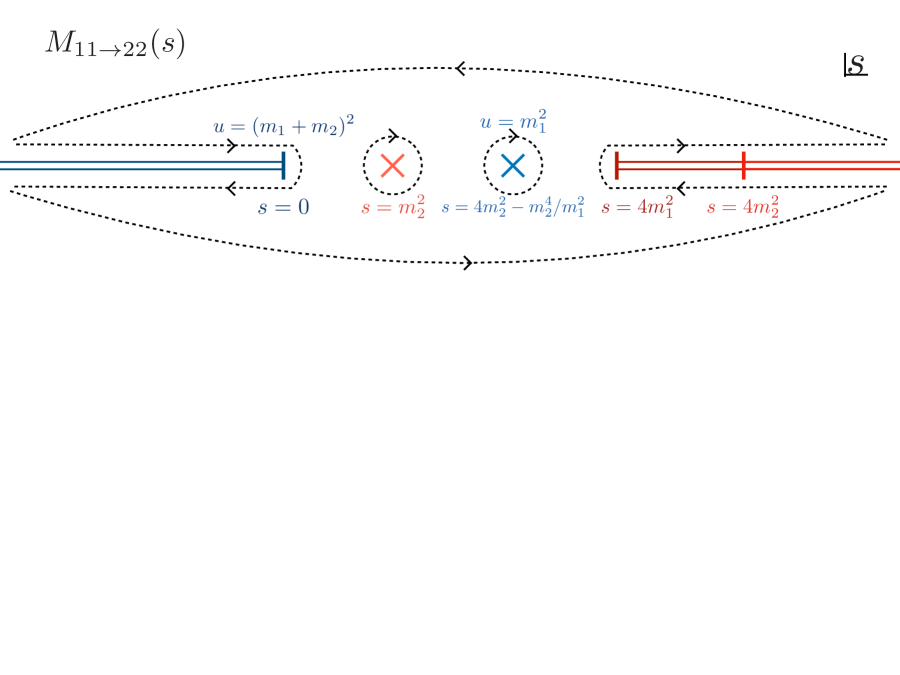
In deriving this relations, see figure 6, we assumed that the scattering amplitudes have no essential singularities at infinity, and in fact approach a constant in this limit, i.e. the S-matrix becomes free. This latter assumption is not crucial nor required: it can be lifted by introducing subtractions as discussed in [2] and the numerical problem of maximising the couplings is not sensitive to this. This is to be expected physically, since the low energy physics of bound state poles should not be much sensitive to the behaviour of the amplitudes at high energies.
To obtain a concrete numerical implementation to the problem, we proceed as follows. First, we define a dispersion grid along the integration domains in (28-31). We then approximate the discontinuities by splines 777If , extended unitarity, equations (22-24), allows for to diverge as close to the threshold. Due to this, between the first two grid points, we approximate . If we should replace in this discussion. linear in between the grid points up to a cutoff point , after which we assume the discontinuities decay as .888This is similar to the numerical implementation in [2]. We could have parametrised our amplitudes using the variables defined in [3]. These variables provide a cleaner framework for the numerics but, in practice, we find that convergence with the variables is much slower than with the use of discretized dispersion relations. With this approximation we can analytically perform the integrals in (28-31) obtaining, in the case and for , as an example,
| (32) |
where the functions are defined in the appendix A of [2]. Next, we impose (27) along a fine grid over (we impose analogous constraints over analogous ranges for the odd channels). Note that we leave for the computer to achieve saturation of (27) before the three-particles thresholds. As shown in appendix I, equation (27)is equivalent to the semidefiniteness constraint
| (33) |
and a similar rewriting can be done for the odd sector. If we fix , as well as the masses, then the matrix in the l.h.s. of (33) is linear on the variables . The problem of maximising in this space of variables under the positive semidefinite constraint (27) (and equivalent for the odd sector) is therefore a semidefinite program and can be solved with, say, SDPB [14]. Details on the numerical implementation, such as parameter settings are available upon request.
3.2 Results for any
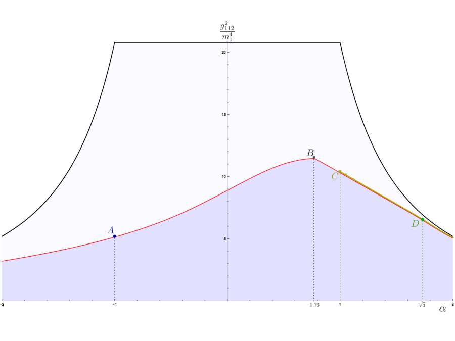
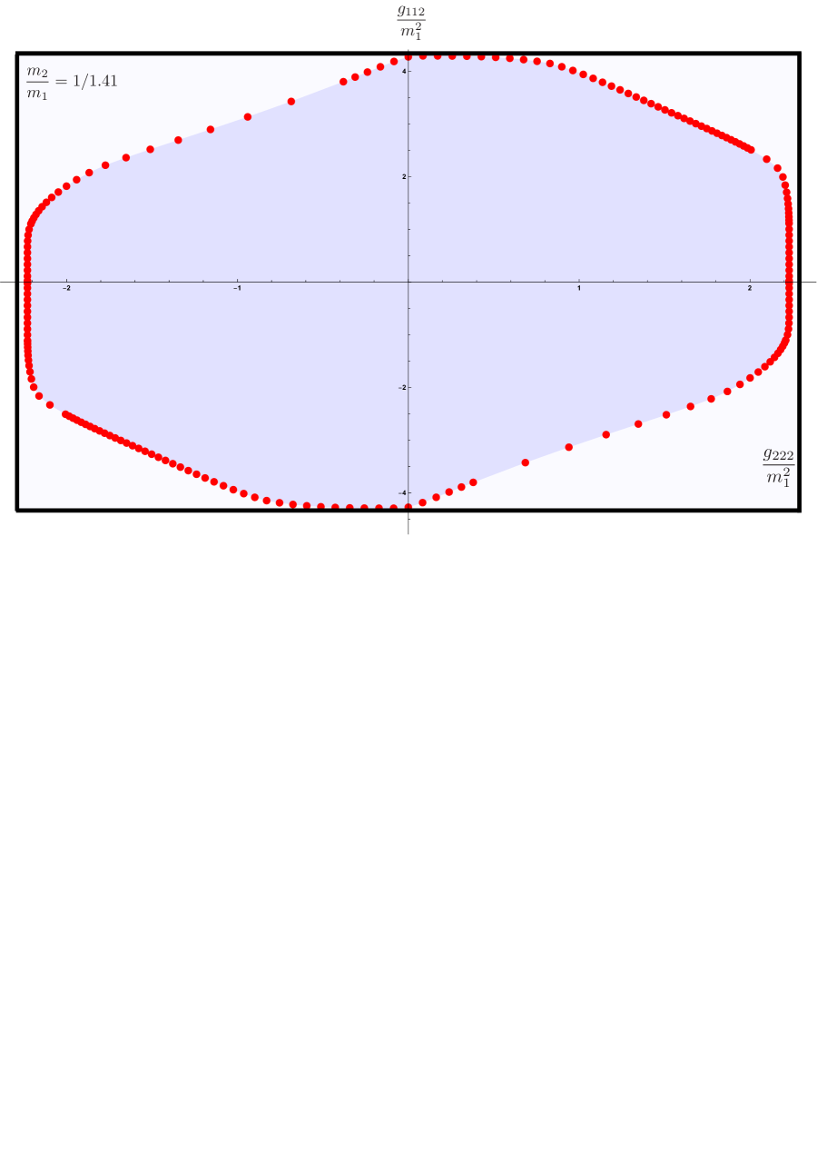
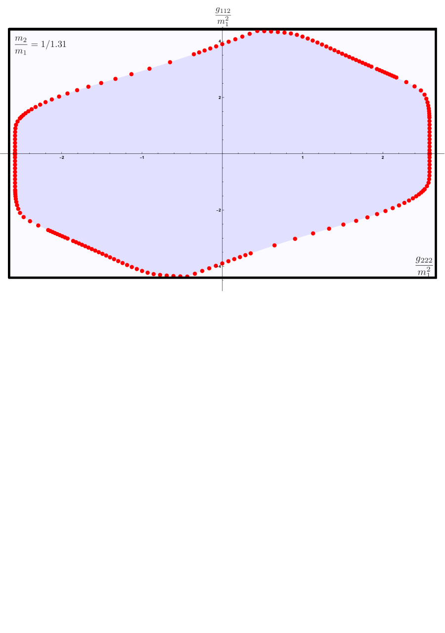
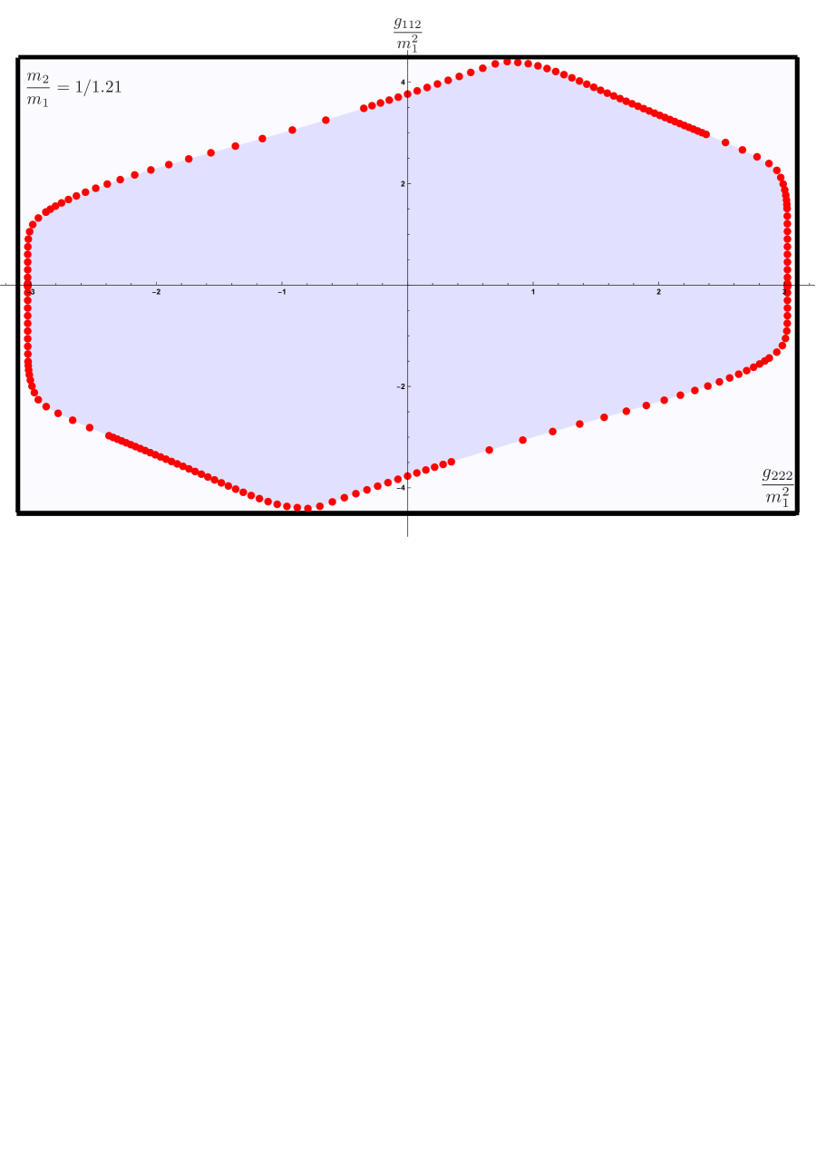
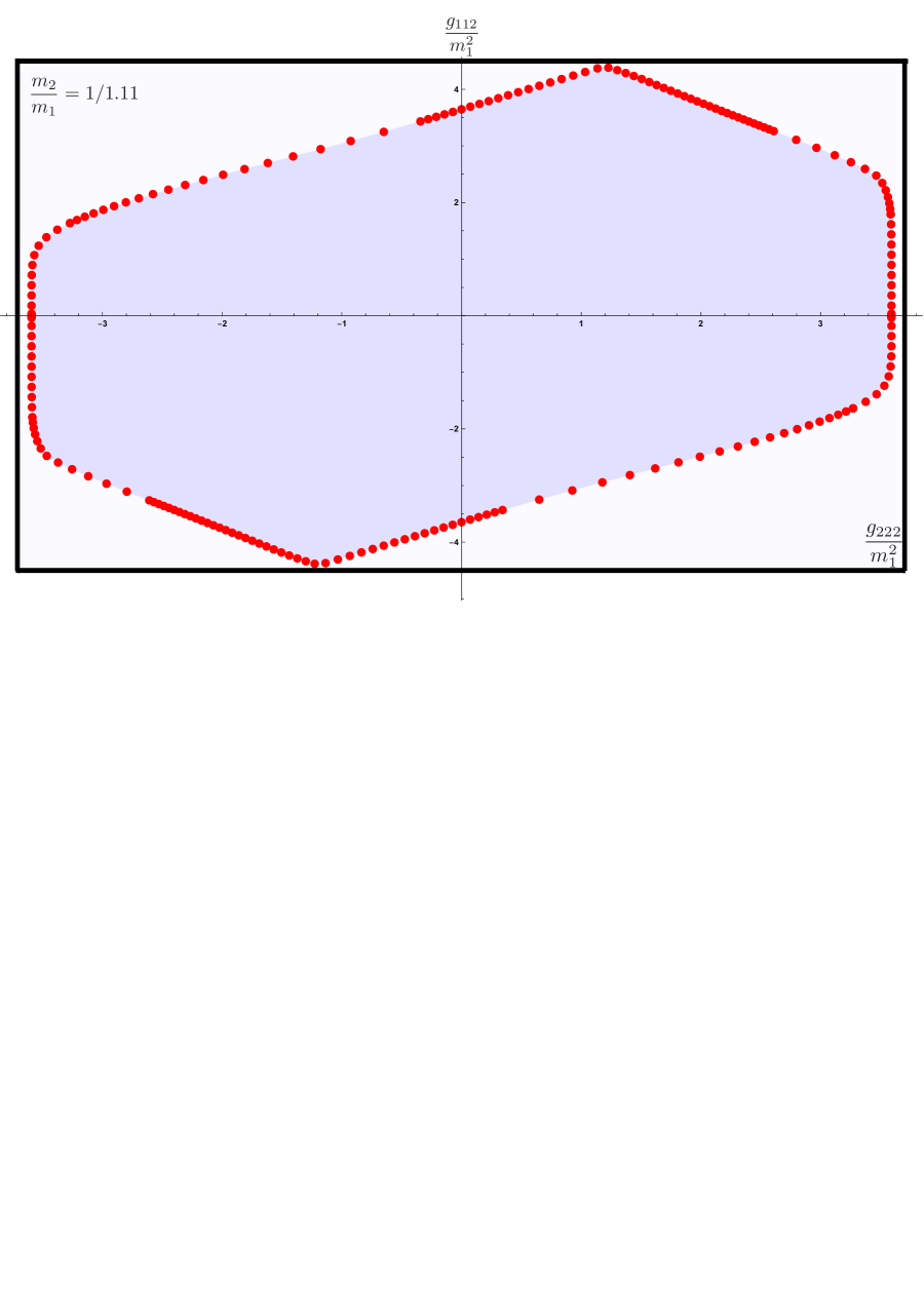
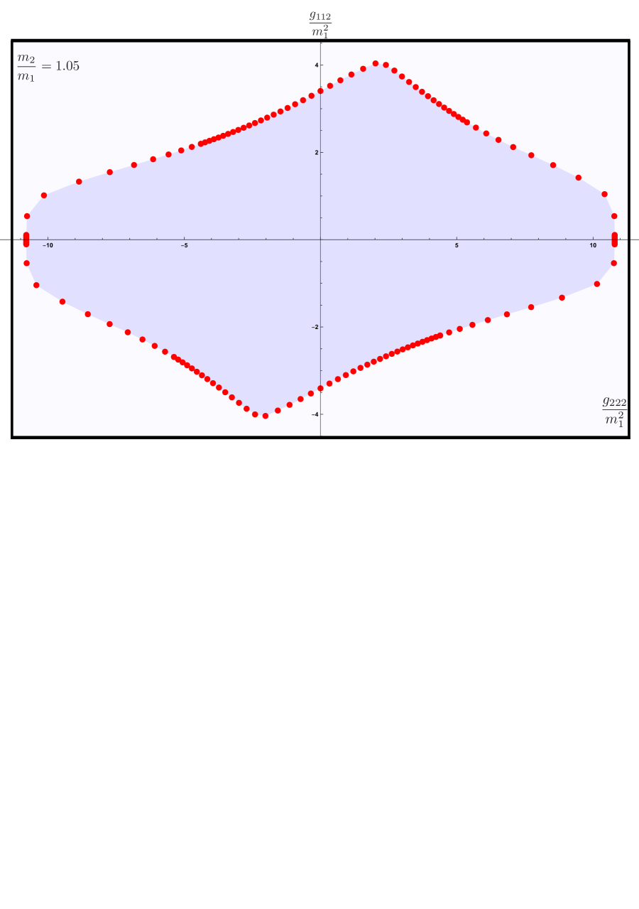
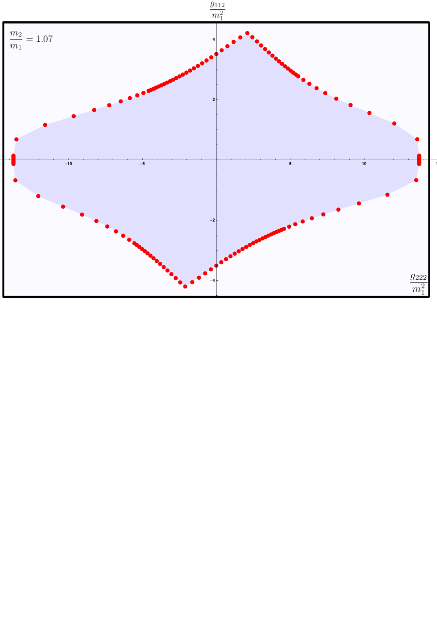
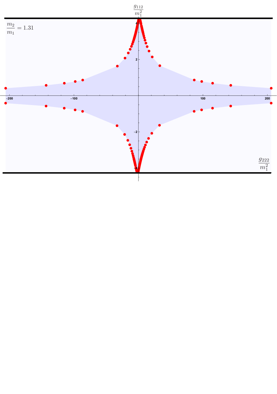
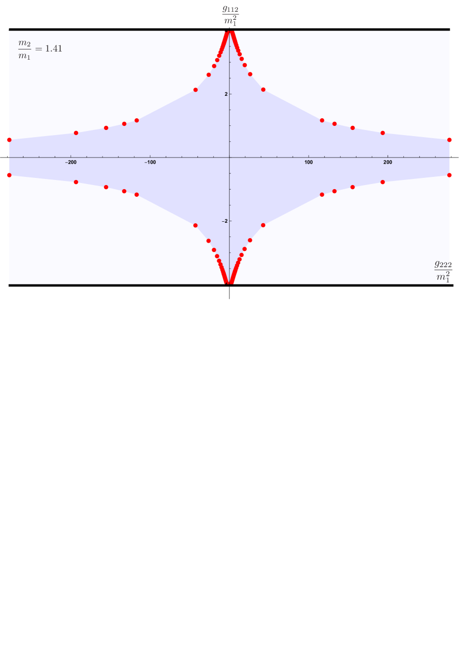
For each mass ratio and for each coupling ratio we can now look for the maximum value of . By varying all parameters we obtain a nice 3D plot which is presented in appendix D; by contrast, in this section we will restrict ourselves to showing only 2D plots that each correspond to a fixed value of . For example, at equal masses we have figure 7 which shows the upper bound as a function of . Although holding fixed is convenient for the numerics (as explained above), it is sometimes more useful to visualize the allowed space of couplings instead. To do this we simply multiply the axis in the numerics by , and in this way we can represent the same data as in figure 9. Applying the same mapping to other mass ratios in the range we furthermore obtain the panels shown in figure 8. (As explained below, the results for are somehow trivial due to screening.) For the most part, the numerical bounds in these figures significantly improve the bounds single amplitude bounds derived in the introduction which set the box sizes.
The most remarkable feature of figures 7 and 8 is the existence of a pronounced maximum of , which is attained for a non-trivial value of the ratio . In particular, for equal masses this maximum (point B in figure 7) is a clear kink in the boundary of the allowed region. It would be remarkable if there is a physical theory sitting close to this kink. As shown in figure 10, such a theory should not be integrable.
Sometimes the numerical red dots in figures 8 approach the solid black lines. When this happens the full numerical bounds saturate the analytically derived diagonal bounds. We see that this happens for very small 999The fact that the numerical points do not exactly touch the vertical lines in panels (a)-(d) in figure 8 when is due to numerical convergence. In that region it would be more sensible to ask for the computer to maximise instead of . This would lead to numerical saturation of the vertical lines. and when we approach the boundaries of the mass range (for some small values of ). This is not surprising: when we decouple the odd and even particles. Since there would be no poles in any amplitude but in , the bound would reduce to the single amplitude bound coming from the process and yielding
| (34) | ||||
| (35) |
This explains the analytic bound in figure 3. In the second case, when we approach the boundary of the mass range, we expect screening to be very important since the extended unitarity region becomes quite large. The poles in the component can now be almost perfectly screened, see also appendix E.2, allowing for the diagonal amplitude bounds on to be saturated. We omitted panels for since in this range we can have perfect screening for any value of , so that the multiple amplitudes bounds in the plane coincide with the rectangular frame derived from diagonal processes.
Note also that there are no vertical walls in the last row of panels in figure 8 since for there are no longer analytic bounds on from the amplitude. As the extended unitarity region in becomes bigger, it becomes increasingly more effective at screening the pole, until at the s (t) channel production threshold collide with the t (s) channel pole as discussed in figure 4. After this mass ratio, the discontinuity across the cut can completely screen the bound state pole implying that its residue can be arbitrary. This is indeed nicely backed up by our numerics as seen in the last two panels in figure 8 where we see that becomes unbounded at this mass range.
Finally, we can also look for the maximum value of either coupling ( or ) leaving the other coupling arbitrary. In other words, how tall () and wide () are the darker allowed regions in (8) where the allowed coupling live. Once plotted for various mass ratios, this gives figures 2 and 3 in the introduction.
Each optimal S-matrix at the boundary of the allowed coupling space is numerically seen to saturate the extended unitarity equations (22-26). This means that the scattering of two particles of type or can never lead to multi-particle production. Processes such as are forbidden. When dealing with 2D S-matrices, in particular extremal examples saturating unitarity such as the ones stemming from this numerical computation, we are commanded to look for integrable field theories. For , these are only possible if the inelastic amplitudes but no -matrices we found satisfy this condition101010This is not an accident, we knew this to be the case apriori since this could only happen if the bound state poles in these amplitudes collided and cancelled or if some extra Landau poles were present. This is not a possibility in the mass range (1). so the boundary S-matrices we find for can at most be close to those describing good physical theories. This still leaves the possibility of finding interesting physical theories along the equal mass line .111111Actually, this line is a one-dimensional kink in the maximal coupling surface described in detail in appendix D.
3.3 (Surprises at) the line
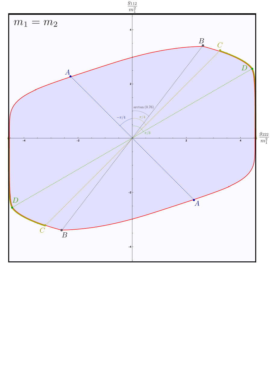
Indeed, nice surprises are to be found in the line depicted in the two equivalent figure 9 (depicting the space of allowed couplings) and figure 7 (for the maximum coupling as a function of the coupling ratio ). Although equivalent these two figures highlight different aspects of this interesting line so it is worth having both in mind.
As concluded in the last section, the line is where our hope lies if we are to match the S-matrices we obtained numerically with physical integrable theories. This necessary condition is not sufficient. For an extremal S-matrix to correspond to an integrable theory it should also obey the factorization conditions encoded in the so-called Yang-Baxter equations [22, 23]. In figure 10 we see how our extremal S-matrices fail to satisfy these conditions as we move along the allowed coupling region (by sweeping ).
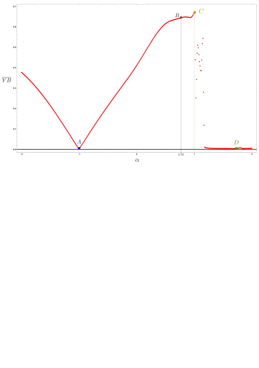
Before unveiling which analytic S-matrices we successfully identified along the line let us go over these numerics in some detail: We observe that for large negative Yang-Baxter is violated until we reach (i.e. when the couplings are equal up to a sign, ) at which point Yang-Baxter is beautifully satisfied. This point is isolated; immediately to the right of Yang-Baxter fails again. It is curious to note that this special point – our first candidate for a physical integrable theory – marked with an in figures 9 and 7 looks absolutely innocent there, without any apparent kink features. As we increase further into positive values we reach point for where the coupling is maximal. As seen in figures 9 and 7 this point is a nice kink. Since it does not obey Yang-Baxter, however, this can hardly correspond to a physical theory. As we increase further we reach marked with a in figures 9 and 7 where again something interesting happens. At that point something goes unstable as far as testing of Yang-Baxter goes indicated by the shower of points in figure 10 from until somewhere around . Once this mess settles we observe a nice line where Yang-Baxter is satisfied throughout! A particularly nice point along that line is point located at . That point actually is the one furthest from the origin in figure 9, in other words, it maximizes and as described below it corresponds to a nice known physical theory.
Now we unveil what we found about these points. In short (setting here):
-
•
Point is a massive deformation of the three state Potts Model.
Here .
-
•
Point is yet to be identified. We do not know the analytic form of the corresponding S-matrix; Since it does not obey YB it can at most be close to a physical theory.
Here .
-
•
Point is (an analytic continuation of the lightest breather S-matrix of) the super-symmetric Sine-Gordon model.
Here .
-
•
There is a line going from point at all the way to where the optimal S-matrix is given by an elliptic deformation of the super-symmetric Sine-Gordon. We are unaware of a physical theory with this S-matrix. Point is the tip of the elliptic deformation where it becomes hyperbolic.
Here .
For comparison recall that the analytic diagonal bounds were .
We will now slowly build up towards those conclusions. The first observation, reviewed in appendix F, is that the full numerical optimization problem can actually be diagonalized and solved exactly for , that is when the two physical couplings are the same up to a sign. For the result is the S-matrix of the massive deformation of the three-state Potts model [19]121212Here we rotated the one particle basis from [19] as , , so that the charge conjugation operator is diagonalized. This operator is to be interpreted as the symmetry generator. In the basis the S-matrix is diagonal and that is why we can solve this point exactly, see Appendix F.
| (36) |
From this solution we read off which matches perfectly with point in figures 9 and 7. In appendix G, we briefly review the 3 state Potts field theory.
As also explained in appendix F, the point is the other point where we can find a clever change of basis to diagonalize our problem and compute the maximal couplings analytically to find which again matches perfectly with point in figures 9 and 7. What we also observe in the process of deriving that analytic solution is that the S-matrix saturating this bound is not unique; there are zero modes. This is probably the explanation of the shower in figure 10. These zero modes are probably only present for but in the vicinity of this point there is probably still some small numerical remnant thereof. We thus expect the shower in figure 10 to be nothing but a zero-mode related numerical artifact; the true solution to the optimization problem probably obeys Yang-Baxter for any . Yet, since this seems to be a zero mode issue, we expect the coupling as predicted by the numerics to still be correct. We will soon provide very strong evidence for these claims.
Point for is a potentially interesting point if we interpret the symmetry as fermion number and think of particles and a Majorana fermion and a boson respectively. Then the condition would follow for theories where these two particles are part of a supersymmetry multiplet, see also [26]. Inspired by this – and by [26] – we tried to compare the optimal S-matrices at to those of the lightest breathers of the super-symmetric sine-Gordon theory.131313Strictly speaking we are comparing with an analytic continuation of that S-matrix since our bound-states have mass equal to the external particles while the next-to-lighests breathers of super-symmetric sine-Gordon have mass bigger than times that of the external particles. In [2] the usual bosonic sine-Gordon S-matrix was identified as the theory with the largest coupling in the S-matrix of the lightest particle with a single bound-state of mass . When this is kosher but as (and in particular for ) we also need to extend the definition of the SG S-matrix beyond its original mass range. In that case it amounted to multiplying the S-matrix by . Here the situation is morally the same but the modification ends up a bit more complicated. This means that here – as there – we do not know a physical theory and we can only write an exact S-matrix that saturates the bound. Beautifully, although we only impose the SUSY condition at the level of the couplings, we see that SUSY emerges at the level of the full S-matrix elements and indeed the optimal S-matrix saturating our bounds at point is an analytical continuation of the lightest breather supermultiplet of the super-symmetric Sine-Gordon! Unfortunately, while we are able to check this to very convincing numerical accuracy we have no analytic derivation of this statement. For completeness, here are some super SG formulae [21].
The lightest breather supermultiplet SSG S-matrix is equal to141414In the basis so that the second (third) element on the second row is the forward (backward) component, for instance.
| (41) |
where
| (42) | ||||
and where is fixed so that the bound state mass is equal to . That is . Note that even though the overall scalar factor in the S-matrix is invariant under , the matrix part is not. This is the sense in which our S-matrix is an analytic continuation of SSG. (compare with SG, in which picking instead of only leads to an overall minus sign). More generally and the physical mass range for SSG is .
Two-particle symmetric solutions of the Yang-Baxter equations are classified [18]. It is natural that if an extension of SSG exists with an extra parameter, that it is given by an elliptic solution of the Yang-Baxter equations. In fact, examining the classified solutions we see that the only good candidate for being promoted to an S-matrix with all the symmetry properties we have and that reduces to SSG in the trigonometric limit is solution 8VII of [18], which is equivalent to
| (47) |
where we normalised by the forward component so that comparison with SSG is easier. from YB. The -channel poles of forward and backward correspond to the flow of a particle of type one, and therefore the residues of this two amplitudes at the pole must coincide. This fixes . Crossing symmetry together with the fact that in the trigonometric limit we have to recover SSG fix where is the complete elliptic integral of the first kind (more precisely, crossing gives with an integer. The limit fixes n). This completely fix a crossing symmetric matrix structure up to one free parameter, , which hopefully is unconstrained. There is a miracle going on. For our amplitudes, we have that
| (48) |
and, moreover,
| (49) |
If (47) is a candidate of matrix structure of the S-matrices saturating the numerical bounds, we must have the same relation between the respective components. It turns out that this holds automatically for any after all the conditions above are imposed. Otherwise this would fix and we would conclude that there are no Yang-Baxter deformations respecting the symmetries and spectrum of our problem. So all we need to do now is to unitarize and introduce the poles. Note that
| (50) |
and for . Therefore, as follows from [2], to unitarize we just need to multiply it by
| (51) |
while to introduce the poles, we multiply by with direct channel pole at ,
| (52) |
At the end of the day, a candidate for a unitary, crossing symmetric, integrable deformation of the supersymmetric sine-Gordon reads
| (53) |
Points and with and would now correspond to and respectively. As , . We can now compute the couplings associated to the elliptic deformation (53), cross our fingers and compare those couplings with the numerics of figures 9 and 7. The elliptic deformation analytic results are the solid chartreuse151515Chartreuse, of selcouth beauty, is a colour half-way between yellow and green. lines in those figures. The agreement could not be better. Note that the agreement goes all the way to point and since by construction the elliptic solution obeys Yang-Baxter, the shower in figure 10 should indeed be a simple zero-mode related numerical artifact. To make precise the elliptic notation used here, we present in appendix J a representation of this S-matrix in Mathematica friendly notation, ready to be copy pasted so the reader can more easily explore this exotic solution.
An obvious question is whether this elliptic deformation corresponds to a nice physical theory.161616We thank Davide Gaiotto for illuminating discussions on related topics. Since the supersymmetric sine-Gordon we encountered here is not a totally kosher theory but an analytic continuation thereof, it is natural to first extend this analysis to the mass range were the super-sine Gordon breather lives and to study its elliptic deformation for those more physical set of parameters. This is beyond the scope of this paper and is currently being investigated in [26].
The line was indeed full of surprises.
4 QFT in AdS
In the previous section we have numerically explored the space of scattering amplitudes that allow for a Mandelstam representation and we found examples of amplitudes that appear to maximize couplings subject to the unitarity constraints. As explained in footnote 1, these extremal coupling constants are not true ‘upper bounds’: although our numerical results appear to have converged, a numerically more refined ansatz will find slightly larger values.
An orthogonal approach to the extremization of three-point couplings in field theories was developed in [1]. The idea is to consider a field theory in an AdS background and investigate the ‘boundary’ correlation functions that are so familiar from the AdS/CFT correspondence. In our setup gravity is non-dynamical and this translates into the absence of a stress tensor among the set of boundary operators. Nevertheless it is natural to claim [1] that these correlation functions obey all the other axioms of a unitary CFT, including crossing symmetry, making them amenable to a numerical bootstrap analysis as in [4]. In this way any general constraints on CFT data directly imply corresponding constraints for QFTs in AdS, and by extrapolating these results to the flat-space limit we can get constraints on flat-space QFTs as well. (For a gapped QFT in AdS2 scaling dimensions and masses are related as and therefore the flat-space limit is typefied by sending all scaling dimensions whilst keeping ratios fixed, .)
The QFT in AdS approach uses CFT axioms to provide rigorous upper bounds, at least modulo our extrapolation procedures. It does not assume analyticity or any particular behavior at large complex energies, and the unitarity constraints are phrased in terms of reflection positivity rather than in terms of probabilities. And yet it was shown in [1] that it provides upper bounds on flat-space couplings that are numerically equal (up to three significant digits in some cases) to the extremal couplings obtained with the S-matrix bootstrap methods. In this section we demonstrate that this striking equivalence was not just a fluke by employing once more the QFT in AdS approach to reproduce some of the previous S-matrix bootstrap results from conformal crossing equations.
4.1 Setup
We will consider four-point functions of operators on the real line, which we think of as the boundary of an AdS2 space with curvature radius . There are two distinguished operators and of dimensions and , which correspond to the two single-particle states of the setup described above – in particular it is understood that for . Besides the assumed symmetry, under which is odd and is even, we will also assume that the QFT is parity invariant and that and are both parity even.171717It is often helpful to think of the parity odd operators as vectors. Indeed, they are equivalent in one dimension because the rotation group is reduced to the parity group and which has only one non-trivial irreducible representation. The OPEs are, schematically,
| (54) |
Here the (non-)appearance of and on the right-hand sides is dictated by symmetry. The other operators are meant to correspond to multi-particle states for the QFT in AdS and their minimal scaling dimension mimicks the beginning of the two-particule cuts in the corresponding scattering amplitudes. The parity properties are dictated by the parity of the operators on the left-hand side. We should add that the OPE coefficients are related to bulk couplings via
| (55) |
with the unsightly relative normalization coefficient [27]
| (56) |
where . This relation was explained in [1].
In one dimension conformal transformations preserve operator ordering modulo cyclic permutations. This leads to the following non-equivalent four-point functions
| (57) |
and we will numerically analyze the lot of them.181818An interesting observation is that the correlator does not feature the identity operator. A conformal bootstrap analysis of this correlator in itself therefore does not give any bounds whatsoever because it lacks an overall normalization. This is completely different from the forward amplitude which we have seen can give a meaningful bound on . However we will shortly see that the ensemble of correlators does give numerical results that mostly agree with the ensemble of amplitudes. Our recipe follows that of [1] with minor variations. Suppose that we wish to obtain a bound on (in units of ) for a given coupling ratio and mass ratio . We then proceed as follows:
-
1.
Choose a . Then set and also fix the ratio
(58) -
2.
A single conformal bootstrap analysis of the four correlators listed above now yields a numerical upper bound on . Our multi-correlator bootstrap analysis is very similar to the one introduced in [12] where it was successfully applied it to the three-dimensional Ising model. The systematics of our analysis (normalizations, conformal block decompositions, functionals) can be found in appendix K. The bound so obtained also depends on the number of derivatives of the crossing equations that we analyze and this introduces a new parameter , so we write
(59) where we use (55) to pass from to .
-
3.
Upon repeating step 2 for various one finds that depends significantly on . To obtain an estimate of the bound that we would obtain if we could analyze all the crossing equations, i.e., if we possessed infinite computational resources, we extrapolate the results for various to estimate
(60) In practice we do this by fitting a polynomial through data points ranging from up to .191919In [1] we were able to obtain results up to or for the different scenarios. The multi-correlator analysis of this paper is numerically more demanding, even more so because the rho series expansion [28] for conformal blocks with large unequal dimensions converges much more slowly. Examples of this extrapolation are shown in figure 26 on page 26. This limit provides our estimate for the best possible upper bound for a QFT in AdS with two particles with masses determined by and and bulk coupling constant ratio given by .
-
4.
We view as a proxy for the AdS curvature radius. We therefore repeat steps to for a number of different values of and once more extrapolate to infinite to obtain a result on the flat-space coupling:
(61) This is the coupling we can compare with the flat-space S-matrix bootstrap analysis.
Appendix K.5 contains technical details of the extrapolation procedure.
For finite and our results provide rigorous upper bounds on the three-point couplings for any QFT in AdS that obeys the stated assumptions. Once we begin the extrapolations we introduce errors that are hard to quantify and this is an unavoidable drawback of our method. Nevertheless we will soon see, as was the case in [1], that the extrapolated bounds appear to accurately reproduce the S-matrix bootstrap results in most cases.
4.2 Results
The numerical algorithm outlined above is computationally demanding. For a single and we need about 10 different values of and for each of these we need about different values of , implying about 150 multi-correlator bootstrap runs. We have therefore chosen a few representative values of and to demonstrate both the feasibility of the multi-correlator conformal bootstrap approach to scattering processes and the match with the flat-space S-matrix bootstrap results.
4.2.1 Results for equal masses
Our first plot is for so we have two particles of equal masses. In figure 11 we overlay the QFT in AdS results (isolated data points) with the S-matrix bootstrap region shown before in figure 9. The black frame again indicates the single-amplitude bounds, which are in fact equal to the single-correlator bounds found in [1]. We have performed a multi correlator QFT in AdS analysis for ratios equal to , , and and in all cases we find reasonably good agreement with the multiple amplitude S-matrix bootstrap result. For our bound comes out somewhat higher than the value reached by the S-matrix bootstrap. This might be due to our extrapolation procedure, which also makes it difficult to put error bars on the QFT in AdS points, but it might also be a consequence of the finite truncation level in the S-matrix bootstrap. It is of course reassuring that the S-matrix bootstrap (Yin) always gives lower values than the conformal bootstrap (Yang).
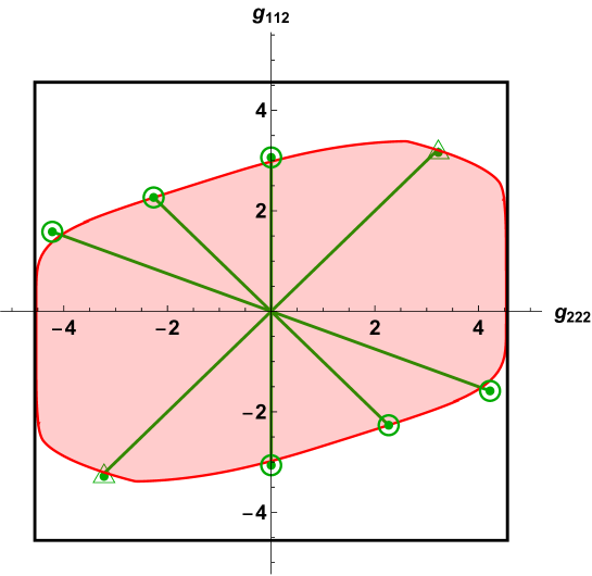
For the ![]() data points in figure 11 the extrapolation is standard, i.e., as outlined above and elaborated on in appendix K, but the
data points in figure 11 the extrapolation is standard, i.e., as outlined above and elaborated on in appendix K, but the ![]() data point requires a comment. In that case we found that the maximal squared coupling from the multi-correlator analysis is always numerically equal to one half of the corresponding maximal squared coupling obtained from the single-correlator analysis – even for finite and so before any extrapolations. Therefore, rather than doing a detailed multi-correlator analysis, we just plotted one half the single-correlator result. This factor of one half is understandable: using a change of operator basis similar to the one described in appendix F, one finds that the multi-correlator problem effectively becomes that of two decoupled single-correlator problems which each feature a squared coupling that is rescaled by a factor 2.202020It is essential here that so .
data point requires a comment. In that case we found that the maximal squared coupling from the multi-correlator analysis is always numerically equal to one half of the corresponding maximal squared coupling obtained from the single-correlator analysis – even for finite and so before any extrapolations. Therefore, rather than doing a detailed multi-correlator analysis, we just plotted one half the single-correlator result. This factor of one half is understandable: using a change of operator basis similar to the one described in appendix F, one finds that the multi-correlator problem effectively becomes that of two decoupled single-correlator problems which each feature a squared coupling that is rescaled by a factor 2.202020It is essential here that so .
4.2.2 Results for
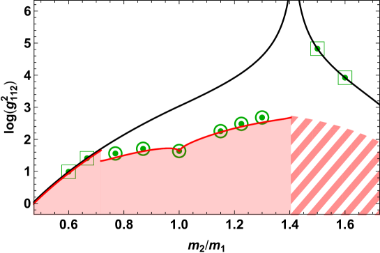
Our next result is shown in figure 12, where we have assumed . We will discuss in turn the black curve, the red shaded region, and the green (new) data points.
The black curve corresponds to the best single-correlator bound for the given mass ratio. It is actually made up of two parts: for it is the bound obtained from the four-point function, whereas for it is the bound obtained from the four-point function. These single-correlator bounds were already obtained in [1] and were shown to agree with the single-amplitude analysis of [2].
In red we show the multi-amplitude results obtained with the methods discussed in section 3.1. It is again made up of different parts: for we can use the numerical analysis and we take the slice from figure 16. For we have screening and the multiple amplitude analysis does not give stronger results than the analysis of the single amplitude which, as we stated before, agrees with the single-correlator bound. For there are Landau singularities and a more sophisticated analysis is necessary to obtain multiple amplitude results, but we do know that the maximal coupling from the multiple amplitude analysis can only lie below the single amplitude bounds. In particular, it must lie below the bound obtained from , which was given as the solid line in figure 2 in the introduction and here yields the striped region in figure 12.212121We explain in appendix L that Landau singularities do not appear in for any mass ratio in the range , so the corresponding single-amplitude bound should be perfectly valid.
Finally, the new data points obtained from the multi-correlator conformal bootstrap are indicated in green. The ![]() data points are obtained from a standard extrapolation, as before, whereas for the
data points are obtained from a standard extrapolation, as before, whereas for the ![]() data points the numerical multi-correlator analysis gave identical results to the numerical single-correlator analysis for all and . The extrapolation will therefore trivially equal the single-correlator result as is indicated in the plot.
data points the numerical multi-correlator analysis gave identical results to the numerical single-correlator analysis for all and . The extrapolation will therefore trivially equal the single-correlator result as is indicated in the plot.
For all points with our extrapolated QFT in AdS results lie at or just above the S-matrix results. As for the previous plot, the small finite difference might be either due to our extrapolation procedure but also due to the S-matrix bootstrap results not yet having converged. The points with are more puzzling. The striped domain, as we mentioned, arises from an analysis of alone and so a multi-amplitude analysis (with Landau singularities and all) will only be able to land somewhere in that domain. Unfortunately this single-amplitude bound does not seem to be picked up by the multi-correlator analysis at all.222222See also footnote 18. It would be nice to know why this is the case: are we missing constraints to be imposed for the QFT in AdS bootstrap?232323At least the multi-correlator result, which is a hard upper bound, is above or equal to the S-matrix bootstrap results in all cases, so the results are not in direct conflict with each other. Alternatively, is there maybe a ‘phase transition’ where by pushing to a very high number of derivatives the single- and multi-correlator analysis begin to differ? Such a phenomenon would obviously invalidate our large extrapolations and might therefore resolve the puzzle. It would be somewhat analogous to the observations discussed in appendix K.4, see in particular figure 25, where we explain that taking different ’s for different crossing equations leads to non-smooth behavior.
Of course, as we mentioned at the beginning of this section, at a technical level the conformal bootstrap analysis looks completely different from the S-matrix bootstrap. We are confident that both analyses yield valid constraints on three-point couplings, but besides physical intuition there was no a priori guarantee that these constraints had to be exactly the same. From this perspective the aspect most in need of an explanation in figure 12 is the quantitative match between the results for (and similarly for all points in figure 11 and the results of [1]) rather than the discrepancy in the other points. Either way, the precise connection between conformal correlators and scattering amplitudes warrants further investigation.
5 Discussion
We have demonstrated the feasibility of the multiple-amplitude bootstrap for the lightest two particles, and shown that it gives stronger bounds compared to the simpler S-matrix bootstrap of only the lightest particle. Clearly one expects to get increasingly stronger bounds by considering more and more scattering processes. It is interesting to consider how such results could converge to an ‘optimal bound’ that we would obtain by considering the entire S-matrix, as follows.
In all our numerical experiments it turns out that the unitarity condition at all energies is (numerically) saturated in the subspace we work on. To illustrate this, consider for example the various possible outcomes from scattering the lightest particle in our setup – let us say that it is the odd particle – against itself. Probabilities must add up to so
| (62) |
where the red and blue inequalities follow trivially from probability positivity as indicated in dark green. In [2] we effectively considered only the weakest red inequality. The theories which lie on the boundary of this space turn out to saturate this inequality for all energies. This would mean that any other process has zero probability, and a theory saturating the bounds of [2] must therefore have zero particle creation or transmutation since the only allowed process is elastic scattering. This is possible for special cases like integrable theories, but generically it cannot be the case. Therefore, by including also the constraints of the other processes we should get better bounds and this is indeed what we have observed in this paper: our improved bounds are due to the stronger constraint given by the lower blue inequality.
However, we once more found that the optimal solutions now saturate this new condition for all values of the energy, so the remaining processes for the extremal S-matrix are again all zero.242424We do not know why this happens; it stands as an empirical observation. In other words, theories lying on the boundary of the new space are theories where particles can continue into or transmute into but we still get zero probability for all other processes that have a different final-state particle content. We expect this pattern to continue by including more and more processes in the game, i.e. we will continue to observe unitarity saturation within the subspace we consider, no matter how large. As we increase the size of our truncation we will hopefully asymptotically approach an optimal bound, but we are unlikely to hit a non-integrable theory at our boundary if we consider only a finite number of processes.252525In particular, the beautiful ridge we observe in figure 16 likely does not correspond to a physical theory in itself, but is hopefully close to one that we can uncover by taking into account more processes. This gives our S-matrix bootstrap approach a more asymptotic flavor than the numerical conformal bootstrap.
Indeed, for our setup with two particles with mass and we find no integrable theories if the masses are different, whereas if they are equal then there are exciting physical theories at our boundary: the three-states Potts model and (an analytic continuation of) the super-symmetric sine-Gordon model. We also find a full segment around the supersymmetric sine-Gordon theory which seems to obey all the necessary factorisation requirements to be an integrable theory; it would be very interesting to see if that is the case. (More on this in [26].)
We also discussed how the same bootstrap results can be obtained from AdS, using the setup first discussed in [1]. Putting a gapped symmetric theory into an AdS box induces a one dimensional symmetric conformal theory in its boundary which we can analyze by numerical conformal bootstrap methods. To make contact with flat space, we take this box to be large which corresponds to large scaling dimensions on the boundary. As it happens the numerical conformal bootstrap results become rather weak at large scaling dimensions and this makes it computationally quite challenging to obtain reliable results. This is the main drawback of the AdS approach. Fortunately there are interesting and potentially very helpful developments on this front: according to [29], convergence can be much improved by a smarter choice of functionals (see also [30, 31]). It would be very interesting to explore this further.
An important advantage of the AdS approach, on the other hand, is that it requires no subtle assumptions about the various analytic properties of scattering amplitudes. The AdS box is thus a literal black box from which we can get beautiful S-matrix bootstrap results even when the analytic properties of such amplitudes might be less obvious.
A good example of such a subtle assumption is extended unitarity, which we have seen is crucial for our multiple-amplitude bounds. Recall that this is a generalisation of usual unitarity which controls the analytic behaviour of scattering amplitudes for unphysical energies, below physical thresholds. For example, when we scatter the next-to-lightest particle against itself we have a two particle cut associated to the lightest particle starting at , before the physical two particle cut at , and extended unitarity governs the discontinuity of scattering amplitudes in the segment between those two values. Extended unitarity is built into perturbation theory [17] but it is not straightforwardly justified non-perturbatively. However, the fact that our QFT in AdS approach exactly reproduces the flat space results provides strong evidence for the validity of the extended unitarity assumption.
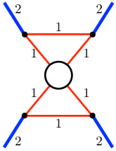
Relatedly, it is puzzling that the AdS bounds for are so much weaker than the forward flat space extremal coupling, see figure 12. Either the AdS numerics did not converge yet or perhaps there is something deeper to be learned there. It would be very interesting to extend our flat space analysis beyond the mass range (1) into the domain. Here we would need to include so-called Coleman-Thun singularities in our setup. An example is shown in figure 13.
Another very important new ingredient which is not unrelated to the anomalous cuts arising in the extended unitarity region and which appeared in this work is the phenomenon of screening. Amplitudes involving heavier particles can sometimes produce discontinuities in some of these anomalous cuts which cancel, i.e. screen, other singularities such as physical poles corresponding to bound-state stable particles. That is, these discontinuities can be tuned so that the amplitudes can often be quite small in the physical energy region where experiments are done. This mechanism is not only possible but it is actually realised by some amplitudes which lie at the boundary of the truncated multiple correlator S-matrix space. It is natural to expect that similar phenomena would also be realised at the boundary of the full S-matrix space. If this boundary is physically significant then screening would be an interesting way for nature to hide strong couplings from the observer.
Let us conclude with some interesting open problems and future directions.
One open problem for which we now have all tools to explore concerns the tricritical Ising field theory. This theory is obtained by deforming a conformal minimal model with two relevant deformations, see appendix H, and is integrable if one of the deformations is set to zero. It would be very interesting to bootstrap this theory when both parameters are non-zero. This is a particularly nice case study because the next to lightest particle here is well below times the mass of the lightest particle – see table 1 for its value at the integrable point – which means we can readily apply all the methods developed here. The only modification would be to include further poles in the ansatz corresponding to the other stable particles this theory has – see again table 1. So here is a homework exercise: consider a line in the mass ratio parameter space which passes by the masses of the integrable theory. Something remarkable should happen: In the anomalous cut of the amplitudes we should see a peak developing as we approach the integrable theory. This peak is going to become a new stable particle in the integrable theory with a mass we know. Seeing this peak show up in detail would be great, as it would constitute a “discovery” of a new particle through the S-matrix bootstrap. Of course, more interesting still would then be to move away from the masses of the integrable theory and explore the full tricritical Ising field theory, non-integrable and all. The previously discovered sharp peak – typical of an integrable theory – would now be smoothened out and correspond to a nearly stable resonance. Because there are so many masses and couplings this would be a challenge numerically, albeit a worthwhile one.
Another open problem which we could now easily address is the problem of multiple amplitudes without symmetry. We would now also include amplitudes such as which have amusing 2D kinematics by themselves. The Ising field theory perturbed by both magnetic field and temperature would be a perfect case study for this case.
A much more challenging but very interesting open problem would be to extend the multiple amplitude analysis to higher dimensions (as in [3] and [10]). The spontaneously broken phase of the model in 3D, for instance, seems to have a single stable bound state of mass [32]; it would be fascinating to try to bootstrap this S-matrix.
Finally, another frontier in 2D would be to delve into the multiple particle S-matrix bootstrap. Can we tame scattering of particles into final particles? There are two obvious obstacles. One is the analytic structure of these amplitudes. They depend now on more kinematical variables and have a huge plethora of Landau singularities; it is unclear if we can characterise them fully. The other challenge is even more basic: can we close up the system of equations? Suppose we consider a basis of initial and final states with both two and three particles. Then we need to deal with the amplitudes. But those, by crossing, are related to . By unitarity we would then need to include four particles in the final and initial states as well. But then we are forced to consider processes which are now related by crossing to and scattering and so on. It seems we are suddenly obliged to consider any number of final particles at once which of course would be computationally completely infeasible. Hopefully we can find a suitable truncation scheme. Along these lines, perhaps we could first try to get some inspiration from the AdS side. Some of the necessary higher point conformal blocks are well known in 1D [33], so can we use this to devise a 1D CFT bootstrap numerical problem dual to the very intimidating flat space multiple particle bootstrap? Even if very challenging numerically, this would prove of extreme conceptual value.
Acknowledgements
We thank Gesualdo Delfino, Carlos Bercini, Lucía Córdova, Patrick Dorey, Davide Gaiotto, Andrea Guerrieri, Matheus Fabri, Giuseppe Mussardo, Miguel Paulos, Erik Schnetter and Alexander Zamolodchikov for numerous enlightening discussions and suggestions. Research at the Perimeter Institute is supported in part by the Government of Canada through NSERC and by the Province of Ontario through MRI. This research received funding from the grant CERN/FIS-NUC/0045/2015. This work was additionally supported by a grant from the Simons Foundation (JP: #488649, BvR: #488659, PV: #488661) JP is supported by the Swiss National Science Foundation through the project 200021-169132 and through the National Centre of Competence in Research SwissMAP.
Appendix A Two dimensions and higher dimensional kinematics
The Mandelstam plane provides us with a very useful depiction of the (real sections of the) interrelations between the three Mandelstam variables . The first important object in this plane is the Mandelstam triangle.
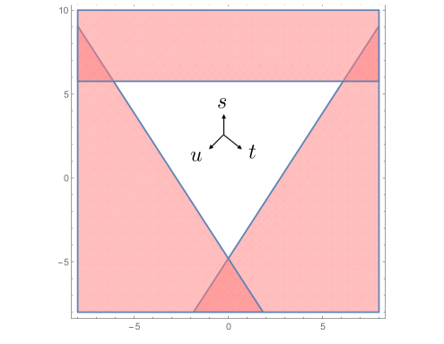
Consider a two-to-two process involving particles with momenta associated to particles of mass . We define the three Mandelstam invariants , and . If particles are the two incoming particles then is the centre of mass energy of the scattering process. The same is true if the incoming particles are particles . In either of these cases the process can only be physical if we have enough energy to produce both the initial and final state, so for . Of course, the same scattering amplitudes can describe other channels.262626To describe other channels we can either swap the masses and always keep to the be the center of mass energy (as in the main text) or leave the masses untouched but reinterpret which Mandelstam invariant corresponds to the center of mass energy (as in this appendix). It is very simple (and very instructive) to go between these active/passive viewpoints. If (or ) are the two incoming particles then is the centre of mass energy of the scattering process and similarly for so the physical conditions in those cases would read and . The three inequalities are depicted by the shaded pink regions in figure 14. The white region is the Mandelstam triangle.
To be in a physical region we thus need to be in the pink region. This is necessary but not sufficient. We need to have enough energy but we also need to scatter at a real angle. For instance for incoming particles we can easily compute the scattering angle to find
| (63) |
For any left hand side between and corresponding to a real angle, and for any in the physical range this equation determines a physical . (Of course, is automatically fixed.) The set of physical and determined in this way determine the physical region in the -channel. The other channels are treated similarly with
| (64) |
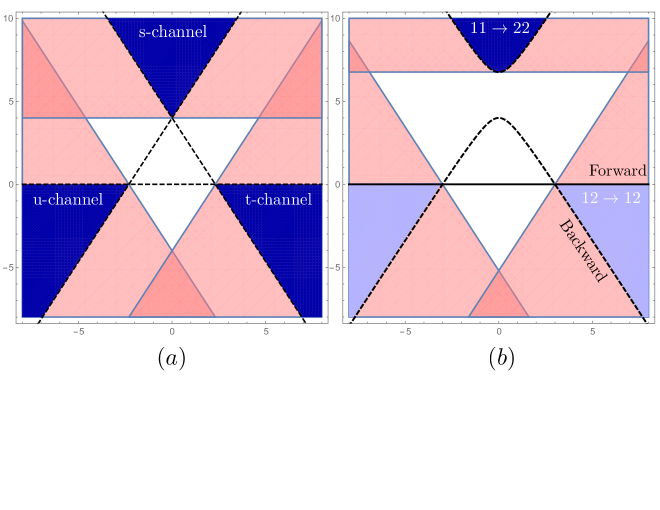
If all masses are equal (to ) then (63) reduces to the famous relation
| (65) |
so that the physical region in the s-channel is simply and represented by the top blue region in figure 15a. In two dimensions the angle ought to be or so that we have either or , i.e. . These two conditions ( and ) are equivalent if the external particles are indistinguishable so in that case we can pick either; in the main text we took . Note that these two conditions are nothing but the boundary of the darker blue region. Similarly we could study all other channels which we can simply obtain by relabelling the Mandelstam variables in (65). The two extra physical regions are the other two blue regions in the same figure 15a. Note that the boundary of all these blue regions can be written concisely as which is nothing but the constraint obtained in the main text from the two dimensional constraint (9) and represented by the dashed lines in figure 15a.
Finally, we come to the more interesting case where the external masses are only pairwise equal: and . This same configuration can describe the process (with being the centre of mass energy), and the processes (with being the centre of mass energy). For the first case we use (63) to get
| (66) |
The physical region corresponding to is now a more interesting curved region, represented by the darker blue region in figure 15b. Again, in two dimensions we can only have backward or forward scattering so must saturate one of these inequalities. If the particles of the same mass are indistinguishable then both solutions are equivalent as before. We can thus take without loss of generality leading to
| (67) |
and reproduce in this way the results below (11) in the main text. In the -channel particles are incoming so we are scattering a odd particle against an even particle. Then we use the first relation in (64) which now reads
| (68) |
Note that in our convention it is (and not ) who is the center of mass energy in this channel.272727Recall footnote 26 when comparing the results that follow to the main text. The physical region corresponding to is now represented by the lighter blue region in figure 15b. The two dimensional conditions that the angle is or are now quite different. The former corresponds to forward scattering and is obtained by (obtained by equating the RHS of (68) to ) while the later corresponds to backward scattering and yields the more involved relation
| (69) |
(obtained by equating the RHS of (68) to .) Note that this relation is nothing but (67) if we solve for . In other words, these two configurations are simply related by crossing symmetry .
To summarize: the boundary of the physical regions are now given by the black solid line and by the black dashed curve in figure 15b. Crossing at relates the left to the right of the straight line – leading to condition (19). Crossing symmetry also relates the top to the bottom branch of the hyperbolic looking curve – reflected in equation (20). In two dimensions these two curves (the hyperbola and the straight line) are independent while in higher dimensions they are smoothly connected (by moving in angle space).
Appendix B Unitarity and final state probabilities
The S-matrix is defined by the expansion of in-states in terms of out-states
| (70) |
The in-states and the out-states are both a complete basis of the Hilbert space. Let us start by discussing the physical meaning of the diagonal unitarity equations (22) and (24). These follow from the statement that the state above is normalized. However, due to the continuum of states this is a bit subtle. The trick is to contract the state with itself but with different momenta
| (71) |
Here, the state represents a state with the same particle content but different momenta. We use the standard normalization for the inner products:
| (72) |
where the product runs over each particle in the state . Unitarity then reads
| (73) |
where is the jacobian defined by
| (74) |
The natural physical interpretation is that
| (75) |
is the probability of the in-state end up in the out-state .
For two particle states and , equation (74) reduces to
| (76) |
with and
| (77) | ||||
| (78) |
This gives
| (79) |
We conclude that, for two particle states, the transition probabilities are given by
| (80) |
For example, for the initial state , we can write
| (81) |
This equation is equivalent to (22) in the energy range
| (82) |
where only 2 particle states are available. To show this we contract (70) with a generic out-state , to find
| (83) |
and use the standard definition of the amplitude :
| (84) |
where denotes the total momentum of the state . This relates with . In the particular case of two particle states one finds
| (85) |
where the first term is present (and equal to ) if and only if the initial and final states are the same. This allows us to rewrite (81) in terms of ,
| (86) |
which should be compared with (22). Notice that the physical derivation given here is not valid for because the two particle state of the heavier particle is not available. This is the regime of extended unitarity where we must use (22).
There is also a more intuitive derivation of the full matrix form of the unitarity constraints (27). Consider the even sector for simplicity. The matrix of inner products of the states :
| (87) |
must be positive semi-definite. In fact, for the range of energies (82) where there are only two particle states, the rank of this matrix must be because both the in and the out states are complete basis. This is a very intuitive way to derive the unitary constraints. However, one must be careful with Jacobian factors that relate different delta-functions. Factoring out and using (70) and (74), we can define a positive semi-definite matrix (without delta-functions)
| (88) |
It is convenient to rescale the states so that all diagonal entries become 1. This leads to the following positive semi-definite matrix:
| (89) |
Notice that using (85), the matrix can be written as
| (90) |
where and are the matrices defined in (27). We will now show that the condition is equivalent to (27) for . First notice that the eigenvalues of the hermitian matrix take the form .282828It is easy to see that the characteristic polynomial is an even function of . Then, the condition implies that . On the other hand, if we compute explicitly the square of , we find
| (91) |
Therefore, the eigenvalues of must be less than 1. Equivalently, we can say that
| (92) |
and (27) follows.292929If a matrix then . This follows from the fact that if for any vector then for any vector (just choose ). In the extended unitarity region this derivation does not apply but we can still use (27).
B.1 Bounding
The discontinuity of the amplitude does not have well defined sign. Furthermore, in the region below the physical regime, one could worry that the discontinuity could be very large and lead to screening. However, the generalized unitarity equations (22)-(24) forbid this phenomena in the range of masses we consider.
For , equations (22-24) reduce to
| (93) | ||||
| (94) | ||||
| (95) |
where the label or stands for the lightest particle. Taking the modulus square of equation (94) and using the other two equations, we find
| (96) |
Therefore the size of is related to the positive discontinuities and , which for this reason are bounded. In fact, in our numerical procedure we impose unitarity as the set of inequalities (27), which in particular implies
| (97) |
This leads to
| (98) |
which bounds in our setup.
B.2 Phase shifts
In the even sector, it is trivial to define diagonal phase shifts
| (99) |
The odd sector is slightly more interesting. In this sector, it is convenient to use states of definite parity,
| (100) |
Then, we define the phase shifts by
| (101) |
In our numerical algorithm, we impose unitarity in the odd sector by the following positive semi-definite condition
| (102) |
It is instructive to see what this implies for the phase shifts . Using (101), we conclude that
| (103) |
where
| (104) |
Thus and we recover the usual unitarity inequality for the phase shifts
| (105) |
Appendix C Analytic upper bound on
The goal of this appendix is to prove that (4) is the amplitude with maximal coupling compatible with crossing symmetry and unitarity. To this end, it is convenient to define
| (106) |
such that
| (107) |
| (108) |
and
| (109) |
Furthermore, is analytic in the -plane minus the s-channel cut and the -channel cut . In the extended unitarity region , we have 303030Recall that .
| (110) |
where we assumed . We conclude that maximizing is equivalent to maximizing subject to , for and for .
To prove that the optimal solution is given by it is useful to change to the coordinate
| (111) |
such that the unit disk covers (the half of) the physical sheet (see figure 1 of [3] for more details). In these coordinates, the optimization problem translates to maximizing subject to for and for , with analytic on the unit disk minus the cut from to 1. Then Cauchy’s theorem leads to
| (112) |
Clearly, the optimal solution is given by (and inside the unit disk).
Appendix D 3D Plots
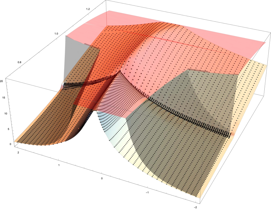
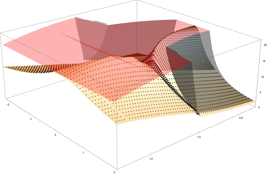
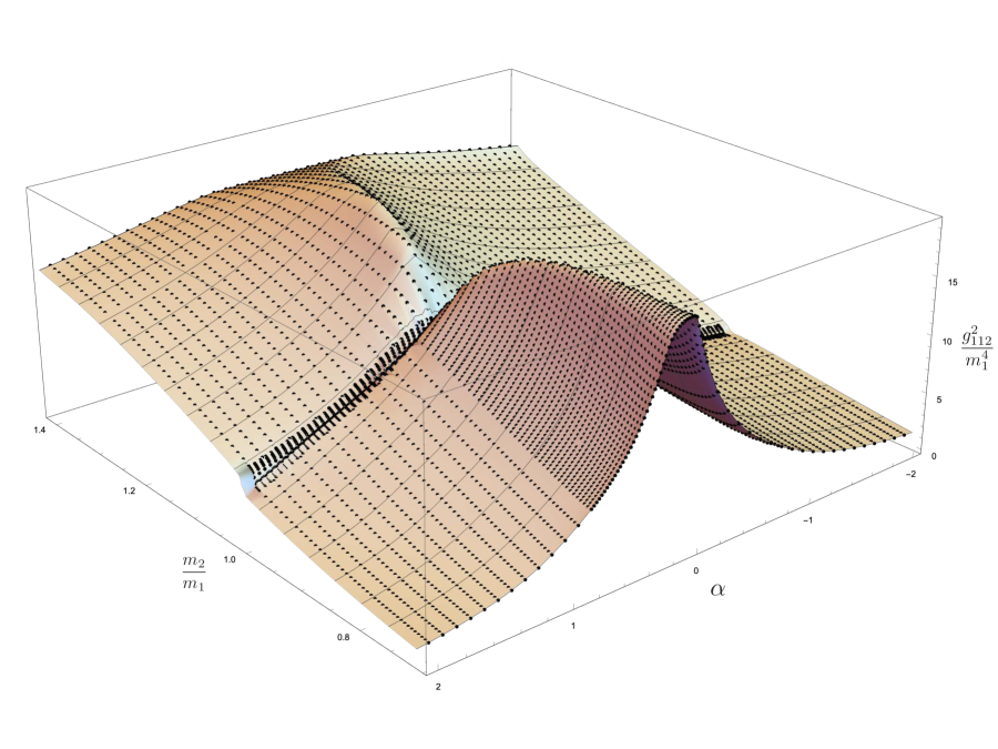
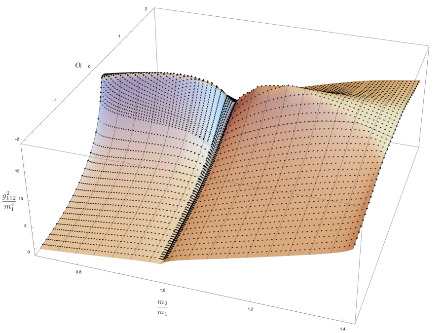
Figure 16 presents the numerical results for the maximum value of for each mass ratio and for each coupling ratio . By changing axes and looking at different sections we obtain figures 8 and 9 from the main text. Many of its features were discussed in section 3.2. The black and red surface correspond to the bounds coming from diagonal processes and are, respectively, the translated versions of the horizontal and vertical solid lines in figure 8.
Figure 16 has a ridge where the coupling is maximal for each mass ratio. That maximal value set an upper bound for the question: how big can the coupling be in a symmetric theory with only two stable particles? In figure 2 we depict this maximum (a similar analysis can be done for , leading to figure 3). We see that this maximal coupling approaches the analytic bound derived from the diagonal component as the mass approaches the boundary of the mass range (1) and is otherwise significantly stronger, specially when the particles are mass degenerate where we observe a nice kink feature in figure 2.
This kink has a cute geometrical interpretation in the full 3d plot in figure 16: The top of the ridge meets a valley at . The valley is a kink for any . For equal masses there is no extended unitarity region and that renders the numerics way more manageable. This is why we can afford to have so many points along the valley as clearly seen in the figure.
There is one more motivation for resolving this valley region very finely: It is the natural place to look for interesting physical theories. Indeed, each optimal S-matrix in the surface of figure 16 saturates the extended unitarity equations (22-26). This means that the scattering of two particles of type or can never lead to multiparticle production. Processes such as are forbidden. When dealing with 2D S-matrices, in particular extremal examples saturating unitarity such as the ones stemming from this numerical computation, we are commanded to look for integrable field theories. For , these are only possible if . It turns out that no point in the surface (16) satisfies this condition.313131This is not an accident, we knew this to be the case a priori since this could only happen if the bound state poles in these amplitudes collided an cancelled or if some extra Landau poles were present. This is not a possibility in the mass range (1). This leaves the possibility of having physical theories along the equal mass line . This line is an one-dimensional kink in the maximal coupling surface described in detail in section 3.3.
Appendix E Screening
E.1 Invisibility Cloak Toy Model
In this appendix we highlight the importance of not leaving any densities unconstrained as they can lead to very efficient screening thus invalidating any possible bounds. To this purpose consider as a toy model the function
| (113) |
where . We think of the first term, the pole at the origin, as a target which we would like to screen. The region where the density term is defined is denoted as the screening region and that second term is denoted as the screening term. We can think of it as an invisibility cloak whose role is to make the full function small in pre-defined regions. To make it concrete suppose we want the target to be screened in a region to the right of the screening region (as we would usually associate to an invisibility cloak a la Harry Potter) but also – thus making it much more challenging – in a region between the target and the screening region and even in another region to the left of the target! The point we want to make here is that this screening is trivial to achieve if we put no bounds on the density . For that purpose it suffices to consider a discretized version of the problem and show that by tuning the ’s we can indeed screen the function remarkably well. Here is an example in Mathematica:
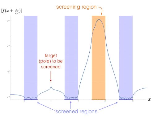
grid=Range[15, 20, 1/5];
screening=Range[25,30,1/10]~Join~Range[-10,-5,1/10]~Join~Range[5,10,1/10];
f[x_]= 1/x + Sum[c[y]/(x - y), {y, grid}];
Total[f[screening]^2]//FindMinimum[#,Variables[#],WorkingPrecision->500]&
leading to the plot in figure 17. Of course this only works because the density is unconstrained here otherwise the amount of possible screening is limited. In the screening region between and the function we get is pretty huge and wild. In other words, the invisibility cloak is working hard so that spectators in the blue screened regions see nothing.
E.2 Screening in our setup
The phenomenon of screening happens in our setup for . In this case, the optimal bounds on the couplings and are just the same as the ones obtained from the single amplitude analysis. In fact, the off-diagonal amplitudes that saturate these bounds vanish in the physical region. To understand how this is possible it is convenient to first understand why the bounds improve in the region .
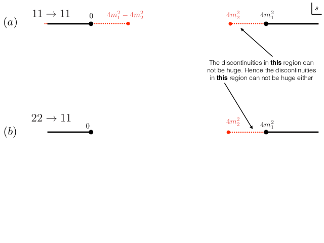
For , the amplitude can not vanish generically so the diagonal amplitude can not saturate unitarity since some production of is inevitable. To see this more precisely note that has poles and an extended unitarity region where the discontinuity is bounded by the diagonal and components as in (98). On the one hand, is bounded by unitarity because this amplitude has no extended unitarity region. On the other hand, the discontinuity of the amplitude is positive in the extended unitarity region and therefore is bounded by unitarity in the physical region. This is depicted in figure 18. To summarize: we see that some screening is possible but it can not lead to a vanishing amplitude in the physical region and thus to unitarity saturation for . This is why the multiple amplitude analysis had to improve the bound obtained from a purely diagonal analysis.
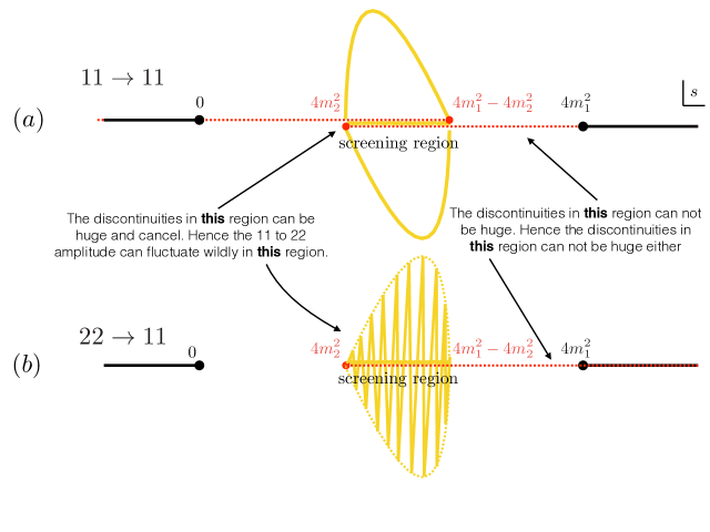
This same analysis also explains why for the diagonal bound is optimal in our setup. This is because in this range we have a collision between the -channel and -channel cuts corresponding to intermediate production of two of the lightest particles in the scattering of the heaviest particle , see figure 19a. The s– and t– channel discontinuities can now be huge as long as they cancel each other and do not lead to a violation of unitarity for the component in the physical region. If they are unbounded, then there is a region in the non-diagonal component where this amplitude can also be unbounded. (Note that if the cuts overlap then the imaginary part in the right hand side of (22) should be understood as the -channel discontinuity.) If the amplitude can be huge with both signs in a finite segment then it can screen as illustrated in the previous section and can thus kill in the physical region (the backward amplitude, related by analytic continuation to the process can also be killed of course). In other words, for we can set to zero all non-diagonal processes without violating any of our physical constraints! Therefore the full numerical plots are expected to coincide with the analytical diagonal bounds. This is indeed what we observed in our numerics.
Would be great to find a way to improve our bounds for . The following section contains a toy model of this screening phenomena which might help elucidate what kind of physics could produce it.
For there is a similar screening phenomena that occurs. Furthermore, in this mass range there are other Landau singularities known in two dimensions as higher pole Coleman-Thun singularities [6]. Indeed, if the mass an on-shell diagram as in figure 13 will produce a double pole. Its residue, as seen in the figure, is governed by the coupling (to the fourth power) and by the on-shell S-matrix of the lightest particle. These are all objects which we are already manipulating and it should thus be possible to tame these singularities if we properly understand how to deal with the inherent non-linearities. We look forward to reporting on this interesting problem in the future.
E.3 Multiple resonance toy model
One might wonder if the screening mechanism is a numerical artifact or could actually be realized in a reasonable QFT. Here we provide an example pointing towards the later provided we accept some fine tuning.
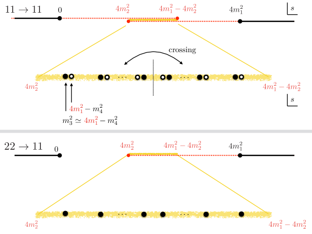
Consider a theory where . The dangerous screening region is the region where the and channel cuts overlap in the amplitude, i.e. for as described in the previous section. Suppose we have many extra even particles with in that screening region range323232Strictly speaking these can not be stable particles since their mass is above so we should think of them as long lived resonances. In other words, we should think of the corresponding poles as coming with a small imaginary part. Our cavalier analysis ignores these subtleties; the conclusions should remain the same since these small imaginary parts are important mostly for the amplitude and for this amplitude we will see that these particles do not show up. and suppose further that for each particle with mass squared in that region there is a particle with mass squared
| (114) |
where is a small parameter. Assume further that the couplings scale with this small parameter as
| (115) |
while since the extra particles are even. Finally, assume that the couplings for two particles related as in (114) are the same up to small corrections. In this scenario, several interesting things might happen, including screening:
-
•
The particles would not appear in the channel since they would come as poles with residues of order or in the channel since they are even.
-
•
The particles would appear in the amplitude. Each particle contributes a huge amount since each coupling is of order . However, because of the condition (114), for each -channel pole there is a corresponding nearby -channel pole which nearly cancels it, leading to a finite result, see figure 20a. If the mass degeneracy if very tiny the couplings could be huge and still lead to a very good cancelation, compatible with unitarity for this amplitude.
-
•
The particles would also appear as s-channel poles in the amplitude since , see figure 20b. Note that this product could be very large and can take any sign. Hence it could lead to screening if is large as explained in the toy example in section E.1. This screening could then lead to being very small in the physical region.
Of course we could ask: “who ordered these extra particles?" No one did but since it is a priori consistent to add them, the numerics will take advantage of them and add them whenever useful for the optimization goal.
Appendix F Solvable Points at
For it is sometimes possible to rotate the one-particle basis as
| (116) |
so that the off-diagonal amplitudes have no poles. If that is the case, we can consistently set these amplitudes to zero and allow for the diagonal processes to saturate unitarity. For the spectrum considered in this paper, the poles terms in the basis are
| (117) |
A straightforward brute force analysis in Mathematica shows that a change of basis as in equation (116) can diagonalise (117) only if
| (118) |
in which case the rotated poles terms become of the form , or
| (119) |
where now the poles terms reduce to . In both cases, the S-matrix in the rotated basis (116) is schematically of the form
| (120) |
It is then straightforward to apply the maximum modulus principle as in section 1 to obtain bounds the optimal couplings. For the (118) scenario, we conclude that and are fixed while , since the diagonal processes must saturate unitarity. This solution corresponds to the S-matrix of the 3-states Potts model at . Note that in the rotated basis we no longer have symmetry for diagonal processes in this case, since the external particles no longer diagonalise the charge conjugation operator, see appendix G. On the other hand, for (119) we conclude only that is fixed and (note that after changing basis is no longer related to by crossing), while and correspond to a zero modes that do not affect the optimal coupling. A particular choice of and lead to the hyperbolic limit of the elliptic deformation of the supersymmetric Sine-Gordon model, discussed in section 3.3.
Appendix G 3-state Potts field theory
The 3-state Potts model in two dimensions has a continuous phase transition described by a non-diagonal minimal model with central charge and a global permutation symmetry . This conformal field theory (CFT) contains 3 relevant scalar operators invariant under (see [25] for a nice introduction to this topic). This allows us to define a family of symmetric QFTs with action
| (121) |
where , and are relevant couplings and we used the notation of [24]. The scaling dimensions of the relevant operators are , and . The purely thermal deformation ( and ) preserves the symmetry and leads to an integrable QFT. This theory has only two stable particles with the same mass transforming as a doublet of . These particles are usually described in a basis where the acts as charge conjugation with [19, 20]. In this basis, the S-matrix is diagonal, i.e. and
| (122) |
where we used the rapidity to parametrize the Mandelstam invariant . Notice that, in this basis, the Yang-Baxter equations are trivially satisfied.
In this paper, we work in the eigenbasis of the global symmetry generated by charge conjugation,
| (123) |
In this basis, we find
| (124) | ||||
| (125) |
Using equation (85) we can obtain the expressions (36) for the connected scattering amplitudes that maximize for and (point A in figure 9).
The magnetic deformations and in (121) preserve and therefore must be compatible with our bounds, at least for small magnetic deformations and that do not give rise to more stable particles. In fact, the mass spectrum of these theories (with and ) has been studied in [24] using the Truncated Conformal Space Approach. The authors observed that the degeneracy between the two particles is lifted for . It would be interesting to study the cubic couplings and the S-matrices of this 2-parameter family of symmetric QFTs and compare them to our bounds.
Appendix H Tricritical Ising (cusp)
The tricritical Ising model in two dimensions has a continuous phase transition described by a diagonal minimal model with central charge and a (spin flip) symmetry. This conformal field theory (CFT) contains 2 relevant scalar operators invariant under (see [25] for a nice introduction to this topic). This allows us to define a family of symmetric QFTs with action
| (126) |
where , are relevant couplings. The scaling dimensions of the relevant operators are and . The purely thermal deformation ( and ) leads to an integrable QFT. This theory has seven particles but only four of them have masses below the continuum of multi-particle states. The masses of these particles are given in table 1.
In this paper, we constrained the space of 2D S-matrices with symmetry by requiring unitarity and analyticity for the two-to-two S-matrix elements involving only the two lightest particles as external states. We restrained ourselves to study the subset of theories for which only and themselves appeared as bound states in these matrix elements. This excludes the tricritical Ising field theory from our analysis in the many body of this paper. However, one can easily relax this restriction. We shall not do a full numerical study of the multiple amplitude bootstrap in this more general setup. We will just derive the analytic bounds that follow from the amplitudes and . For concreteness, we consider a theory with symmetry and a mass spectrum as in the table 1.333333 Any masses within the range and would lead to qualitatively the same conclusions regarding single amplitude bounds as below but the precise locations of cusps and edges on the bounds does depend on the masses. If we deviate away from these mass constraints then we we would have to redo the analysis. This is the same discontinuous nature of the bounds already observed in [2], see e.g. figures 10 and 11 therein.
| Particle | Mass | charge |
|---|---|---|
| odd | ||
| even | ||
| odd | ||
| even | ||
| + possibly extra particles with masses bigger than . |
With this setup there is a richer structure of couplings to play with. For example, in the amplitude we have bound state poles corresponding to particles and :
| (127) |
where . One question that could be asked is: what values for the pair are allowed by the unitarity constraint ?
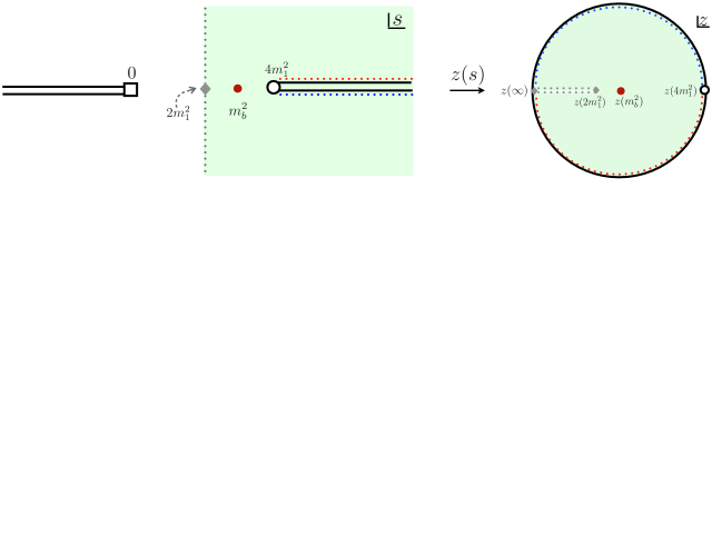
To answer this question, it is useful to introduce the variables
| (128) | ||||
| (129) | ||||
| (130) |
where we take for convenience. This choice of maps to and the imaginary axis to . See figures 21 and 22 for an illustration of such maps.
As a function of the variable, has poles at and . Therefore the function
| (131) |
is a holomorphic function on the unit disk which satisfies, as a consequence of unitarity, . Moreover, from the fact that has a negative residue at and a positive residue at , we find that is positive at and .
Suppose we want to maximise . This is equivalent to maximising . But by the maximum modulus principle, everywhere inside the unit disc and, moreover, the optimal value is only achieved when . From the fact that is positive at and we conclude that a maximal is obtained for and
| (132) |
Note that this solution also maximises so that
| (133) |
Now we maximise under the extra constraint that with . This maximisation problem (together with the equivalent problem of maximising with fixed) completely determines the subspace of compatible with , since this space is convex.
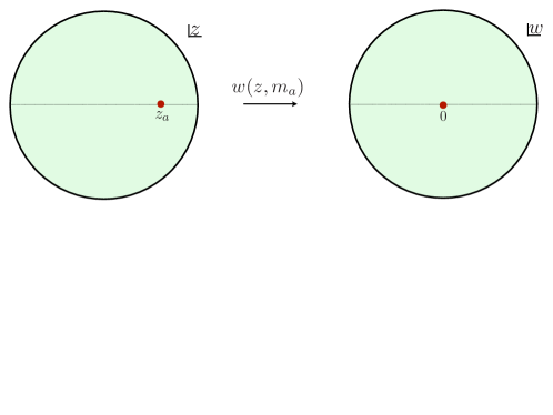
Under this extra constraint, we know that and so the solution is no longer possible. Consider, however, the function
| (134) |
where we now think of as a function of by inverting equation 130. Since is an increasing function of , to maximise is equivalent to maximise . Moreover, since is an automorphism of the disk, unitarity implies for on the unit disc. Finally, . Now recall Schwartz Lemma:
Lemma 1
Schwartz Lemma: Let be the unit disk and be a holomorphic map such that and on . Then . Moreover, if the inequality is saturated for any non-zero point in , then with .
We conclude that under the extra constraint , the maximal value for is given by the solution of the following algebraic equation on :
| (135) |
After performing the equivalent exercise for the maximisation of under , where , we obtain the allowed space of as depicted in the figure 23.
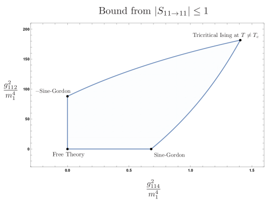
One can play the same game for the matrix element, which contains bound state poles corresponding to particles and (and therefore constrain the space . One can then combine both results into a plot of allowed triplets compatible with and . This is figure 24.
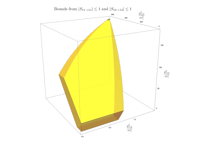
It would be interesting to perform a multiple amplitudes analysis for this setup and explore the space of masses in the vicinity of the values of table 1. Notice that in such an analysis, the values in table 1 would be single out by the condition that the multiple amplitude bounds saturate the single amplitude bounds of figure 24 at the tip of the spear. That is because only for those particular masses can the multiple poles in the off-diagonal channels coincide and cancel (à la integrable bootstrap), allowing for the off-diagonal amplitudes to vanish and for the diagonal processes to saturate unitarity, as in the boundary of the yellow surface in figure 24. It would also be interesting to see if the sub-leading (non-integrable) deformation of the tricritical Ising model leads to any feature of the bounds.
Appendix I Numerical optimization as a SDP
As discussed in section 3.1, once we fix , our discretised ansatz for the amplitudes depends only on the variables . To reduce the maximisation problem to an SDP, all we need to do is to write the extended unitarity constraint (27) as a semidefinite constraint linear on , as in (33). The purpose of this appendix is to prove the equivalence of (27) and (33) or, explicitly,
| (136) |
Appendix J Elliptic Deformation
Bellow one can find the definition of the supersymmetric sine-Gordon elliptic deformation S-matrix in Mathematica friendly notation.
w = EllipticK[k]/\[Pi];
e = 1;
g = 2 \[Pi]/3;
ED = {{JacobiDN[g w, k] - (JacobiDN[I q w, k] JacobiSN[g w, k])/(e
JacobiCN[I q w, k] JacobiSN[I q w, k]), 0, 0,
(JacobiDN[I q w, k] JacobiSN[g w, k])/(e JacobiCN[I q w, k])},
{0, 1, -(JacobiSN[g w, k]/(e JacobiSN[I q w, k])), 0},
{0, -(JacobiSN[g w, k]/(e JacobiSN[I q w, k])), 1, 0},
{(JacobiDN[I q w, k] JacobiSN[g w, k])/(e JacobiCN[I q w, k]), 0, 0, -JacobiDN[g w, k]
- (JacobiDN[I q w, k] JacobiSN[g w, k])/(e JacobiCN[I q w, k] JacobiSN[I q w, k])}};
IntR[x_, k_] := 1/(2 \[Pi] I)Block[{w = (EllipticK[k]/\[Pi])},
(NIntegrate[Log[((1 - JacobiSN[g w, k]^2/JacobiSN[I q w, k]^2)^ -1)
/Sinh[q]^2]/Sinh[q - x], {q, -Infinity, Infinity}])];
U[x_, k_] := -I Sinh[x] Exp[IntR[x, k]];
CDDPole[q_] := (Sinh[q] + I Sin [g])/(Sinh[q] - I Sin[g])
SED[Q_, K_] := U[Q, K] CDDPole[Q] ((ED /. w -> EllipticK[k]/\[Pi])
/. {k -> K, q -> Q});
Note that to compute the S-matrix for physical , one must be careful and take the appropriate principal value around the singularity at in the integrand of IntR.
Appendix K Conformal computations
K.1 Crossing symmetry in one dimension
We consider correlation functions of primary operators in a one-dimensional boundary field theory. The weight of the operator will be denoted as . We will work in the Euclidean theory on . The conformal group is a two-fold cover of ; its elements act by the usual fractional linear transformations on the positions,
| (142) |
with . The elements with negative determinant involve the parity transformation . The Jacobian of this transformation is and the fields transform as
| (143) |
with dictated by the parity of .343434The parity operator is unitary and its square is an internal symmetry transformation. Up to a well-known caveat [34, section 3.3] we can always redefine the parity operator so it squares to and its eigenvalues are then as we assumed. In a correlation function we should remember that the parity operation also reverses the operator ordering.
In a suitable basis the two-point functions take the familiar form
| (144) |
The two-point function of a parity odd operator is negative, so the associated norm is positive.353535It may help the reader that parity odd operators are the same as one-dimensional vectors . The reflection-positive two-point function is then , in one dimension.
The operator product expansion reads
| (145) |
where we assume that . If we act with the parity operator on both sides then we find
| (146) |
and therefore the reflected OPE coefficients between primaries are
| (147) |
with
| (148) |
The previous relation in particular implies that parity odd operators can never appear in the OPE of two identical operators. We will work in a basis where two-point functions are diagonal. The structure of three-point functions then dictates that
| (149) |
and so the OPE coefficients transform either in the trivial representation (if ) or the sign representation (if ) of the permutation group . Notice that, even if parity is broken, the cyclic symmetry is always preserved. This for example means that , whereas and are not always the same.
We will be specifically interested in four-point functions,
| (150) |
with, as usual, and
| (151) |
If for then . The -channel conformal block decomposition reads
| (152) |
with the conformal blocks
| (153) |
where we added an absolute value sign so the expression is unambiguous also for negative values of its argument.
Let us briefly discuss operator ordering. Correlation functions with operator orderings that are cyclic permutations of each other are directly related, as follows from covariance under the (orientation-preserving) inversion . Furthermore, parity symmetry dictates that
| (154) |
To see the complications that arise if we just swap two adjacent operators, let us swap operators 1 and 2. A simple relabeling leads to the block decomposition
| (155) |
and assuming a parity invariant theory this is equal to
| (156) |
where we used a standard hypergeometric transformation formula, valid for . The factor and the absolute value sign in the definition (153) imply that and are not, in general, related in an obvious manner. The symmetries and non-symmetries altogether leave us with three independent four-point functions from which the others follow. We can take these to be , , and , which respectively correspond to , , and . We will here be interested in just the second of these correlators.
With the ordering fixed there are only two OPE channels. For the ordering we gave the first one above; the crossed channel OPE reads
| (157) |
with . Crossing symmetry then takes the form363636One foolproof way to obtain this expression is to relabel the operators in the original expression (150) and then use a conformal transformation to relate to . To verify that directly fusing operators 2 and 3 together in (150) gives the same OPE limit requires that which we proved previously.
| (158) |
Let us consider all correlation functions of two parity-even operators and . We then find, in a diagonal operator basis, the following set of non-trivial crossing equations:
| (159) |
where the operators labeled are parity even, whereas the operators labeled can be either parity even or parity odd.
K.2 Transition to convex optimization
In matrix form, the ’th crossing symmetry equation can be written as:
| (160) |
with
| (161) |
and with
| (162) | ||||||
where
| (163) |
We can act with a functional on each equation, and then add all of them. This yields
| (164) |
where (without an argument) is shorthand for the function of obtained by acting with the corresponding component of the functional.
If we single out the identity (with and ) and the external operators from the sums then we obtain
| (165) |
For a feasibility study we can normalize the functionals on the unit operators, giving
| (166) |
and furthermore demand positive semidefiniteness of the three square matrices listed above. We can also get bounds on products of OPE coefficients. For example, if we set
| (167) |
and then maximize/minimize , we obtain a lower/upper bound on . More precisely, if we extremize and the result is positive then crossing cannot be solved. If the result is negative then the absolute value of the result is our upper (for minimization) or lower (for maximization) bound.
K.3 Setup with symmetry
In the previous section we discussed the general one-dimensional conformal bootstrap analysis for two operators. Let us now specialize to the case discussed in the main text, so we consider a QFT in AdS2 with a symmetry and only two stable parity even particles; a odd one created by an operator and a even one created by an operator .
With this additional symmetry automatically which leaves four non-trivial correlation functions of and . In these correlators we should also label the internal operators with an even/odd quantum number depending on the OPE channel in which they appear. Our notation above is already adapted to this situation: in equation (159) the operators labeled are necessarily parity and even, whereas the operators labeled are parity even or odd but always odd. (Operators that are even but parity odd do not feature in this set of correlation functions.) With the exception of and themselves we take their dimensions to lie above the following ‘gap’ values:
| gap | index in (168) | ||
|---|---|---|---|
| even | even | ||
| odd | even | ||
| odd | odd |
These gaps are precisely the two-particle values for a QFT in AdS, reflecting our assumption that there are no further stable single-particle states.
Going then through the same logic as before we write the crossing equations in matrix form as
| (168) |
with (note some redefinitions with respect to the previous formulae)
| (169) |
and with
| (170) |
After acting with the functional and singling out the important operators again we find
| (171) |
If we want to find bounds in the plane we can set and set a normalization
| (172) |
With this normalization our problem takes the form of a semidefinite program and we can proceed using the well-known numerical bootstrap methods of [4, 12] and the specialized solver of [14]. Further technical details are available upon request from the authors.
K.4 Functionals and derivative combinations
As in previous works, our choice of functionals are linear combinations of derivatives of the crossing equations at , so our functionals can be written as
| (173) |
The coefficients should be thought of as the main degrees of freedom to be fixed by the optimization procedure. Furthermore, in a multi-correlator study we can act with a different functional on each of the crossing equations in (159), so the degrees of freedom are
| (174) |
where, as before, denotes the different crossing equations and we used that the third and fourth equation are identically zero by our symmetry assumptions.
Of course the functions that are odd around , like the first and second crossing equation in (159), contribute only about non-trivial degrees of freedom since the for odd are meaningless (and in fact should be set to zero to prevent numerical instabilities). This reduces the scaling of the number of components to rather than .
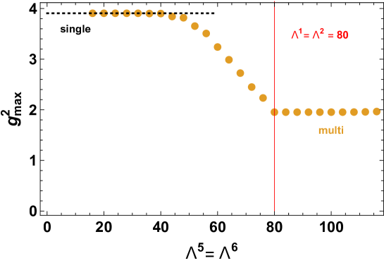
In our earliest attempts we thought it unfair to first two crossing equations that they could only contribute half as many functional components as the fifth and sixth equation. Therefore we decided to cut off the sum in (173) at for the fifth and sixth equation but at for the first and second equation. Such an egalitarian approach, however, would have led to completely different and incorrect results. To illustrate this we plot in figure 25 the upper bound on the coupling as a function of , i.e. the cutoffs for the fifth and sixth equation, whilst holding fixed every other parameter, including the cutoffs for the first and second equation. Clearly for the multi-correlator bound offers exactly no improvement over the single-correlator bound. So, if we had continued to work with the egalitarian cutoffs then we would erroneously conclude that no improvement would have been possible over the single-correlator bound! Only when increasing beyond do we begin to see a gradual improvement, which stops as abruptly as it started at .
Notice that the plot is drawn for the ![]() data point in figure 11, which has the special property that the multi-correlator bound turns out to be exactly half that of the single-correlator bound. We however observed very similar behavior, including the kinks and stabilization, also for other data points where the final multi-correlator bound is completely non-trivial.
data point in figure 11, which has the special property that the multi-correlator bound turns out to be exactly half that of the single-correlator bound. We however observed very similar behavior, including the kinks and stabilization, also for other data points where the final multi-correlator bound is completely non-trivial.
K.5 Extrapolations
An example of the extrapolation procedure outlined in section 4.1 is shown in figure 26. One important subtlety not mentioned in the main text is that we extrapolate the log-ratio of the multi-correlator and the single-correlator result. That is, for every multi-correlator optimization run we also ran a single-correlator optimization run (for either or ) and so we get raw data that we can denote and . We found that direct extrapolation of the multi-correlator bounds led to a relatively large dependence on our fitting procedure, whereas extrapolation of the log-ratio
| (175) |
could, as shown, be done with relatively low-degree fits. Since we know that the single-correlator bounds match the analytic single-amplitude bounds with large accuracy [1], we can add (the logarithm of) this known answer to our extrapolated log-ratio to obtain a better estimate of the flat-space multi-correlator bound.
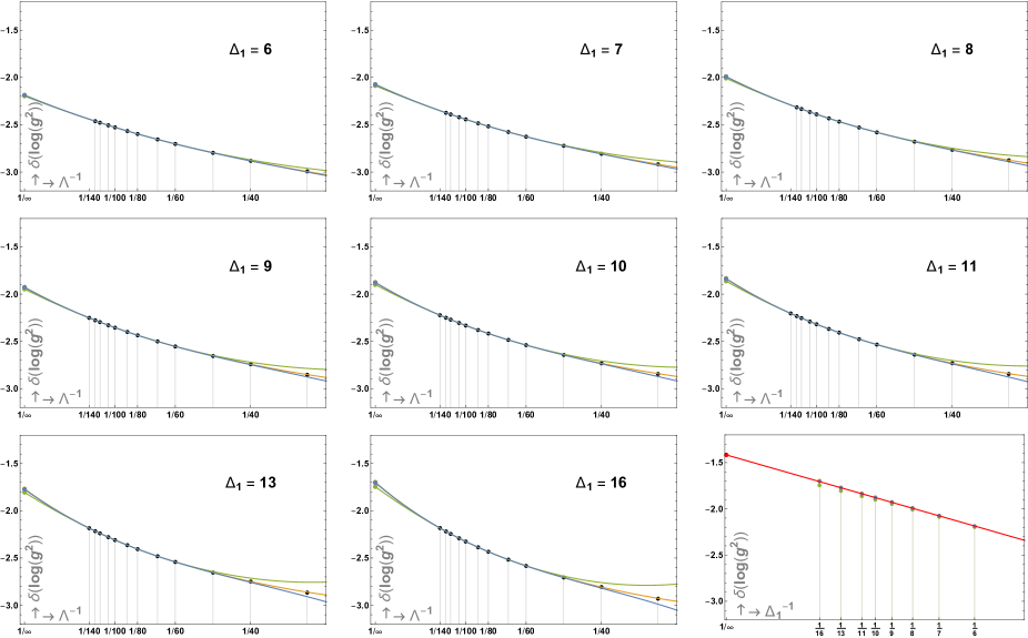
The first 8 plots show the raw data and subsequent extrapolations to infinite . The three curves correspond to fits with a polynomial in of degree 3 (in blue), degree 4 (in orange, mostly coinciding with blue), and degree 2 (in green). In the fits we did not include the (three) data points with . We observe a rather small difference between the different extrapolations, and we have checked that these fits give good predictions for the high raw data points if we exclude one or more of them by hand.
The final plot in figure 26 collects all the extrapolated points to infinite . The data points line up nicely, providing evidence for a small non-systematic error in our first extrapolation. We have fitted a linear function in to the degree 3 (in blue) points, leading to the extrapolated value of for the log-ratio of this data point. From this plot it is clear that there is no meaningful difference if we had extrapolated the degree 4 (in orange) points instead.
We employed exactly the same extrapolation procedure, including the choice of the degree of the fitting functions, for all the other data points shown in the main text.
Appendix L Landau Singularities in Scattering
Landau singularities are associated to diagrams representing particle interactions with all lines on-shell and momentum conservation at each vertex [17, 6]. We claimed in the text that for the forward scattering there ought to be no new such singularities (to be added to the bound state poles already there) whereas for the backward component we claimed that when we do find such new on-shell processes. It is easy to convince oneself of that with a few pictures. For that purpose, we adapt here some beautiful discussion in chapter 18 of the book [35] by Bjorken and Drell, translating it to our two dimensional case of interest.
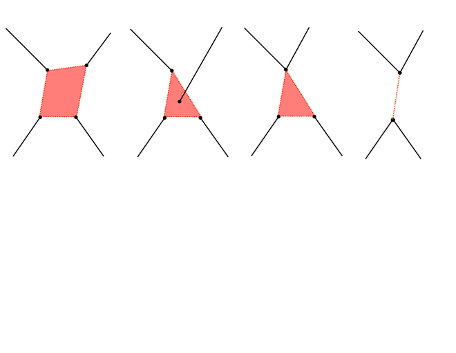
Start with a diagram representing a two-to-two on-shell process. Each of the four external particles eventually encounter a vertex (several can meet at the same vertex). Consider those vertices containing an external line. They define a convex hull which can be a quadrilateral, a triangle or a line as shown in figure 27. Next we draw all other internal lines to complete the Landau diagram. The first important claim is that all those lines must lie inside the convex hulls just defined. That is simply because of momentum conservation: if they got out of the convex hull there would be no external particle to kick them back in (and the diagram would never close)! With this in mind we can go on to analyse the three possible convex hulls in turn.
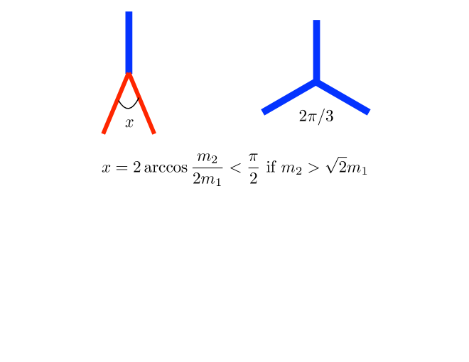
Consider first the quadrilateral case and assume first that at each of the four external vertices we have a cubic vertex. Then, momentum conservation and on-shellness constrains the angles at those cubic vertices373737In this appendix we assume that the diagrams and four-momenta are euclidean. This is the case in-between two-particle cuts, since then all spatial momenta can be chosen to be purely imaginary, making the lorentzian metric effectively euclidean. The absence of Landau diagrams in the full physical sheet follows from their absence in the euclidean region after a causality argument, as detailed in [35].. For example, for the case at hand with two particles of different masses we have the angles in figure 28. For we realize right away that the angles are obtuse so it is generically impossible to form a quadrilateral! What about using other vertices when particles first interact? Well, that would be even worse as the total opening angles would be even greater in that case. If then one of the angles is smaller than so we have a better chance of finding extra singularities and, indeed, we can sometimes form such diagrams, as the one in figure 13, but not if two external particles are of type and two particles are of type as illustrated in figure 29(a). Hence, there are no “quadrilateral convex hull" Landau diagrams for scattering.
What about “triangular convex hull” singularities? When , as explained in figure 29(b), those are indeed present in the backward component, but not in the forward one. So the backward amplitude should have extra Landau poles but the forward amplitude should not. As such, the bound on derived from the forward component should hold even for . As discussed in the main text, this bound is not captured by the QFT in AdS bootstrap, see figure 12.
We did not discuss the case where the convex hull is the line: those are just the usual singularities such as the bound state poles and all the production cuts which open for multi-particles at rest, and thus moving parallel to each other, along the convex hull line.
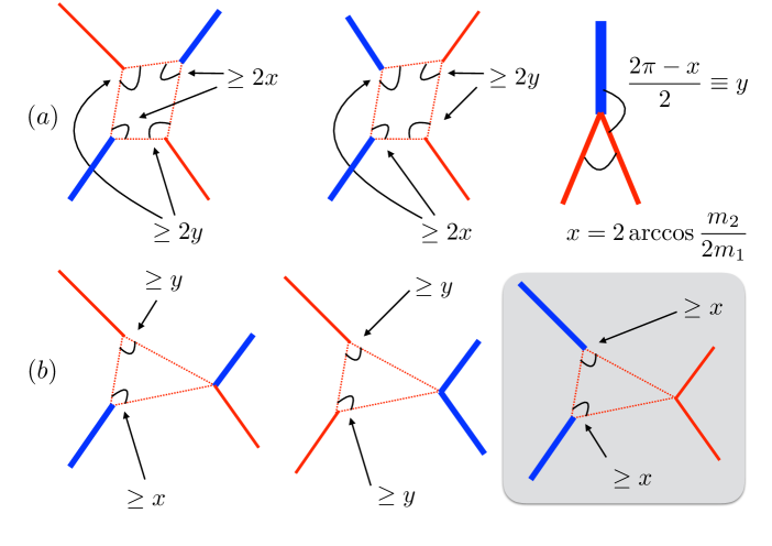
References
- [1] M. F. Paulos, J. Penedones, J. Toledo, B. C. van Rees and P. Vieira, “The S-matrix bootstrap. Part I: QFT in AdS,” JHEP 1711 (2017) 133 doi:10.1007/JHEP11(2017)133 [arXiv:1607.06109 [hep-th]].
- [2] M. F. Paulos, J. Penedones, J. Toledo, B. C. van Rees and P. Vieira, “The S-matrix bootstrap II: two dimensional amplitudes,” JHEP 1711 (2017) 143 doi:10.1007/JHEP11(2017)143 [arXiv:1607.06110 [hep-th]].
- [3] M. F. Paulos, J. Penedones, J. Toledo, B. C. van Rees and P. Vieira, arXiv:1708.06765 [hep-th].
- [4] R. Rattazzi, V. S. Rychkov, E. Tonni and A. Vichi, “Bounding scalar operator dimensions in 4D CFT,” JHEP 0812 (2008) 031 doi:10.1088/1126-6708/2008/12/031 [arXiv:0807.0004 [hep-th]].
- [5] F. Caracciolo and V. S. Rychkov, “Rigorous Limits on the Interaction Strength in Quantum Field Theory,” Phys. Rev. D 81, 085037 (2010) doi:10.1103/PhysRevD.81.085037 [arXiv:0912.2726 [hep-th]].
- [6] S. R. Coleman and H. J. Thun, “On the Prosaic Origin of the Double Poles in the Sine-Gordon S Matrix,” Commun. Math. Phys. 61, 31 (1978). doi:10.1007/BF01609466
- [7] Y. He, A. Irrgang and M. Kruczenski, “A note on the S-matrix bootstrap for the 2d O(N) bosonic model,” JHEP 1811 (2018) 093 doi:10.1007/JHEP11(2018)093 [arXiv:1805.02812 [hep-th]].
- [8] L. Córdova and P. Vieira, “Adding flavour to the S-matrix bootstrap,” JHEP 1812 (2018) 063 doi:10.1007/JHEP12(2018)063 [arXiv:1805.11143 [hep-th]].
- [9] M. F. Paulos and Z. Zheng, “Bounding scattering of charged particles in dimensions,” arXiv:1805.11429 [hep-th].
- [10] A. L. Guerrieri, J. Penedones and P. Vieira, “Bootstrapping QCD: the Lake, the Peninsula and the Kink,” arXiv:1810.12849 [hep-th].
- [11] F. Kos, D. Poland and D. Simmons-Duffin, “Bootstrapping the vector models,” JHEP 1406 (2014) 091 doi:10.1007/JHEP06(2014)091 [arXiv:1307.6856 [hep-th]].
- [12] F. Kos, D. Poland and D. Simmons-Duffin, “Bootstrapping Mixed Correlators in the 3D Ising Model,” JHEP 1411, 109 (2014) doi:10.1007/JHEP11(2014)109 [arXiv:1406.4858 [hep-th]].
- [13] D. Poland, S. Rychkov and A. Vichi, “The Conformal Bootstrap: Theory, Numerical Techniques, and Applications,” Rev. Mod. Phys. 91 (2019) no.1, 015002 doi:10.1103/RevModPhys.91.015002 [arXiv:1805.04405 [hep-th]].
- [14] D. Simmons-Duffin, “A Semidefinite Program Solver for the Conformal Bootstrap,” JHEP 1506, 174 (2015) doi:10.1007/JHEP06(2015)174 [arXiv:1502.02033 [hep-th]].
- [15] M. Creutz, “Rigorous bounds on coupling constants in two-dimensional field theories,” Phys. Rev. D 6, 2763 (1972). doi:10.1103/PhysRevD.6.2763
- [16] K. Symanzik, “The asymptotic condition and dispersion relations,” In: Lectures on field theory and the many-body problem, pp. 67-92, Caianiello, E.R. (ed.). New York: Academic Press 1961
- [17] L. D. Landau, “On analytic properties of vertex parts in quantum field theory,” Nucl. Phys. 13 (1959) 181. doi:10.1016/0029-5582(59)90154-3 R. E. Cutkosky, “Singularities and discontinuities of Feynman amplitudes,” J. Math. Phys. 1 (1960) 429. doi:10.1063/1.1703676
- [18] K. Sogo, M. Uchinami, Y. Akutsu, M. Wadati, “Classification of exactly solvable two-component models," Prog. Theor. Phys. 68 (1982) 508. doi: 10.1143/PTP.68.508
- [19] A. B. Zamolodchikov, “Integrals of Motion in Scaling 3-State Potts Model Field Theory," Int. J. Mod. Phys. A, 03, (1988) 743. doi:10.1142/s0217751x88000333
- [20] M. Caselle, G. Delfino, P. Grinza, O. Jahn and N. Magnoli, “Potts correlators and the static three-quark potential,” J. Stat. Mech. 0603 (2006) P03008 doi:10.1088/1742-5468/2006/03/P03008 [hep-th/0511168].
- [21] C. Ahn, “Complete S-matrix of Supersymmetric Sine-Gordon Theory and Perturbed Superconformal Minimal Model" Nucl. Phys. B 354 (1991) 57. doi:10.1016/0550-3213(91)90175-W
- [22] C. N. Yang, C. P. Yang, “Thermodynamics of one-dimensional system of bosons with repulsive delta function interaction," J. Math. Phys. 10 (1969) 1115
- [23] A. B. Zamolodchikov, Al. Zamolodchikov, ‘Factorized s Matrices in Two-Dimensions as the Exact Solutions of Certain Relativistic Quantum Field Models," Annals Phys. 120 (1979) 253
- [24] L. Lepori, G. Z. Toth and G. Delfino, “Particle spectrum of the 3-state Potts field theory: A Numerical study,” J. Stat. Mech. 0911 (2009) P11007 doi:10.1088/1742-5468/2009/11/P11007 [arXiv:0909.2192 [hep-th]].
- [25] G. Mussardo, “Statistical field theory : an introduction to exactly solved models in statistical physics,”
- [26] C. Bercini, M. Fabri, A. Homrich, P. Vieira, “2D SUSY S-matrix Bootstrap Kinks”
- [27] D. Z. Freedman, S. D. Mathur, A. Matusis and L. Rastelli, “Correlation functions in the CFT(d) / AdS(d+1) correspondence,” Nucl. Phys. B 546, 96 (1999) [hep-th/9804058].
- [28] M. Hogervorst and S. Rychkov, “Radial Coordinates for Conformal Blocks,” Phys. Rev. D 87, 106004 (2013) doi:10.1103/PhysRevD.87.106004 [arXiv:1303.1111 [hep-th]].
- [29] M. F. Paulos, B. Zan, “A functional approach to the numerical conformal bootstrap," [arXiv:1904.03193[hep-th]]
- [30] D. Mazac, M. F. Paulos, “The analytic functional bootstrap. Part I: 1D CFTs and 2D S-matrices," JHEP 1902,162 (2019) doi:10.1007/JHEP02(2019)162 [arXiv:1803.10233 [hep-th]]
- [31] D. Mazac, M. F. Paulos, “The analytic functional bootstrap. Part II. Natural bases for the crossing equation," JHEP 1902,163 (2019) doi:10.1007/JHEP02(2019)163 [arXiv:1811.10646 [hep-th]]
- [32] M. Caselle, M. Hasenbusch, P. Provero, K. Zarembo “Bound states in the 3-d Ising model and implications for QCD at finite temperature and density," Nucl. Phys. Proc. Suppl. 106 (2002) 504-506 doi:10.1016/S0920-5632(01)01761-3 [arXiv:0110160v1 [hep-lat]]
- [33] V. Rosenhaus, “Multipoint Conformal Blocks in the Comb Channel," JHEP 1902,142 (2019) doi:10.1007/JHEP02(2019)142 [arXiv:1810.03244 [hep-th]]
- [34] S. Weinberg, “The Quantum theory of fields. Vol. 1: Foundations”
- [35] J.D. Bjorken, S. Drell, “Relativistic Quantum Fields”