Naive Bayes with Correlation Factor for Text Classification Problem

Abstract

Naive Bayes estimator is widely used in text classification problems. However, it doesn’t perform well with small-size training dataset. We propose a new method based on Naive Bayes estimator to solve this problem. A correlation factor is introduced to incorporate the correlation among different classes. Experimental results show that our estimator achieves a better accuracy compared with traditional Naive Bayes in real world data.

I Introduction

Text classification problem has long been an interesting research field, the aim of text classification is to develop algorithm to find the categories of given documents. Text classification has many applications in natural language processing (NLP), such as spam filtering, email routing, and sentimental analysis. Despite intensive work, there still remains an open problem today.

This problem has been studied from many aspects, including: supervised classification problem, if we are given the labeled training data; unsupervised clustering problem, if we only have documents without labeling; feature selection.

For supervised problem, if we assume that all the categories follow independent multinomial distributions, and each document is a sample generated by that distribution. Then a straight forward idea is to use some linear models to distinguish them, such as support vector machine (SVM)[1, 2], which is used to find the ”maximum-margin hyper-plane” that divides the documents with different labels. The algorithm is defined so that the distance between the hyper-plane and the nearest sample $d_{i}$ from each group is maximized. The hyper-plane can be written as the set of documents vector $\vec{d}$ satisfying:

$$\vec{w}\cdot\vec{d}-b=0,$$

where $\vec{w}$ is the normal vector to the hyper-plane. Under the same assumption, another effective classifier, using scores based on the probability of given documents conditioned on categories, is called Naive Bayesian classifier[3, 4, 5]. This classifier learns from training data to estimate the distribution of each categories, then we can compute the conditional probability of each document $d_{i}$ given the class label $C_{i}$ by applying Bayes rule, then the prediction of the class is done by choosing the highest posterior probability. The algorithm to get the label for a given document $d$ is given by:

$$label(d)=\operatorname*{argmax}_{j}P(C_{j})P(d|C_{j}).$$

Given a huge data set, we also consider using deep learning models such as Recurrent Neural Network (RNN)[6, 7] to do classification, which includes more information such as the order of words and semantic representations.

For unsupervised problem, we have traditional method SVD (Singular Value Decomposition)[8] for the dimension reduction and clustering. There also exist some algorithms based on EM algorithm, such as pLSA (Probabilistic latent semantic analysis)[9], which considers the probability of each co-occurrence as a mixture of conditionally independent multinomial distributions:

$$P(w,d) = \sum_{C}P(C)P(d|C)P(w|C)$$

$$= P(d)\sum_{C}P(C|d)P(w|C),$$

where $w$ and $d$ are observed words and documents, and $C$ is the words’ topic. As mentioned above, parameters here are learned by EM algorithm. Using the same idea, but assuming that the topic distribution has sparse Dirichlet prior, we have algorithm LDA (Latent Dirichlet allocation)[10]. The sparse Dirichlet priors encode the intuition that documents cover only a small set of topics and that topics use only a small set of words frequently. In practice, this results in a better disambiguation of words and a more precise assignment of documents to topics.

Naive Bayes estimator is a widely used estimator, however, it requires plenty of well labeled data for training purposes. To tackle this problem, this paper proposes a novel estimation method. In the remainder of this paper, we firstly summarize the Naive Bayes estimator in section III. Then we discuss the error of the Naive Bayes estimator in Theorem III.1 and demonstrate that it is unbiased. In section IV, we propose a novel estimation method (see equation 11) called Naive Bayes with correlation factor. It addresses the problem in many real world text classification applications that have only limited available training data. Furthermore, in theorem IV.1 we show the error of the new estimator is controlled by the correlation factor and the variation has a smaller order compared with Naive Bayes estimator. In section V, we show results of simulations, which demonstrates the performance of our method presented in section IV. Finally section VI concludes our work and mentions possible future work.

II General Setting

Consider a classification problem with the sample (document) set $S$, and the class set $C$ with $k$ different classes:

$$C=\{C_{1},C_{2},...,C_{k}\}.$$

Assume we have totally $v$ different words, thus for each document $d\in S$, we have:

$$d=\{x_{1},x_{2},\cdots,x_{v}\}.$$

Define $y=(y_{1},y_{2},\cdots,y_{k})$ as our label vector. For document $d$ is in class $C_{i}$, we have $y_{i}(d)=1$. Notice that for a single label problem, we have: $\sum_{i=1}^{k}y_{i}=1$.
For a test document $d$, our target is to predict:

$$\hat{y}(d)=f(d;\theta)=(f_{1}(d;\theta),f_{2}(d;\theta),...,f_{k}(d;\theta))$$

given training sample set $S$, where $\theta$ is the parameter matrix and $f_{i}(d;\theta)$ is the likelihood function of document $d$ in class $C_{i}$.

III Naive Bayes classifier in text classification problem

In this section we will discuss the properties of estimator derived from traditional Naive Bayes method. Let class $C_{i}\;(1\leq i\leq k)$ with centroid $\theta_{i}=(\theta_{i_{1}},\theta_{i_{2}},...,\theta_{i_{v}})$ and $\theta_{i}$ satisfies: $\sum_{j=1}^{v}\theta_{i_{j}}=1$. Assuming independence of the words, the most likely class for a document $d$ is computed as:

$$label(d) = \operatorname*{argmax}_{i}P(C_{i})P(d|C_{i})$$

$$= \operatorname*{argmax}_{i}P(C_{i})\prod_{j=1}^{v}(\theta_{i_{j}})^{x_{j}}$$

$$= \operatorname*{argmax}_{i}\log{P(C_{i})}+\sum_{j=1}^{v}x_{j}\log{\theta_{i_{j}}}.$$

This gives the classification criteria once $\theta$ is estimated, namely finding the largest among

$$\log f_{i}(d;\theta)=\log{P(C_{i})}+\sum_{j=1}^{v}x_{j}\log{\theta_{i_{j}}}\;\quad 1\leq i\leq k$$

Now we shall derive an maximum likelihood estimator for $\theta$. For a class $C_{i}$, we have the standard likelihood function:

$$L(C_{i},\theta) = \prod_{d\in S}f_{i}(d;\theta)^{y_{i}(d)}$$ (2)

$$= \prod_{d\in C_{i}}\prod_{j=1}^{v}\theta_{i_{j}}^{x_{j}}$$

Take logarithm for both sides, we obtain the log-likelihood function:

$$\log{L(C_{i},\theta)}=\sum_{d\in C_{i}}\sum_{j=1}^{v}x_{j}\log{\theta_{i_{j}}}.$$ (3)

We would like to solve optimization problem:

$$\max\ \log L(C_{i},\theta)$$ (4)

$$\text{subject to}: \sum_{j=1}^{v}\theta_{i_{j}}=1$$

$$\theta_{i_{j}}\geq 0$$

The problem (4) can be explicitly solved by Lagrange Multiplier, for class $C_{i}$, we have $\theta_{i}=\{\theta_{i_{1}},\theta_{i_{2}},...,\theta_{i_{v}}\}$, where:

$$\hat{\theta}_{i_{j}}=\frac{\sum_{d\in C_{i}}x_{j}}{\sum_{d\in C_{i}}\sum_{j=1}^{v}x_{j}}.$$ (5)

For estimator $\hat{\theta}$, we have following theorem.

Theorem III.1

Assume we have normalized length of each document, that is: $\sum_{j=1}^{v}x_{j}=m$ for all documents $d\in S$, the estimator (5) satisfies following properties:

1. $\hat{\theta}_{i_{j}}$ is unbiased.

2. $E[|\hat{\theta}_{i_{j}}-\theta_{i_{j}}|^{2}]=\frac{\theta_{i_{j}}(1-\theta_{i_{j}})}{|C_{i}|m}$.

Proof:

With assumption $\sum_{j=1}^{v}x_{j}=m$, we can rewrite (5) as:

$$\hat{\theta}_{i_{j}}=\frac{\sum_{d\in C_{i}}x_{j}}{\sum_{d\in C_{i}}m}=\frac{\sum_{d\in C_{i}}x_{j}}{|C_{i}|m}.$$

Since $d=(x_{1},x_{2},...,x_{v})$ is multinomial distribution in class $C_{i}$, we have: $E[x_{j}]=m\theta_{i_{j}}$, and $E[x_{j}^{2}]=m\theta_{i_{j}}(1-\theta_{i_{j}}+m\theta_{i_{j}}).$

1. $$E[\hat{\theta}_{i_{j}}] =E[\frac{\sum_{d\in C_{i}}x_{j}}{|C_{i}|m}]=\frac{\sum_{d\in C_{i}}E[x_{j}]}{|C_{i}|m}$$

   $$=\frac{\sum_{d\in C_{i}}m\theta_{i_{j}}}{|C_{i}|m}=\theta_{i_{j}}.$$

   Thus $\hat{\theta}_{i_{j}}$ is unbiased.

2. By (1), we have:

   $$E[|\hat{\theta}_{i_{j}}-\theta_{i_{j}}|^{2}]=E[\hat{\theta}_{i_{j}}^{2}]-2\theta_{i_{j}}E[\hat{\theta}_{i_{j}}]+\theta_{i_{j}}^{2}=E[\hat{\theta}_{i_{j}}^{2}]-\theta_{i_{j}}^{2}.$$

   Then notice

   $$\hat{\theta}_{i_{j}}^{2}=\frac{(\sum_{d\in C_{i}}x_{j})^{2}}{|C_{i}|^{2}m^{2}}=\frac{\sum_{d\in C_{i}}x_{j}^{2}+\sum_{d\neq d^{\prime}\in C_{i}}x_{j}^{d}x_{j}^{d^{\prime}}}{|C_{i}|^{2}m^{2}},$$ (6)

   where $d=(x_{1}^{d},x_{2}^{d},...,x_{v}^{d})$.
   Since:

   $$E[\frac{\sum_{d\in C_{i}}x_{j}^{2}}{|C_{i}|^{2}m^{2}}] =\frac{|C_{i}|m\theta_{i_{j}}(1-\theta_{i_{j}}+m\theta_{i_{j}})}{|C_{i}|^{2}m^{2}}$$

   $$=\frac{\theta_{i_{j}}(1-\theta_{i_{j}}+m\theta_{i_{j}})}{|C_{i}|m},$$

   and

   $$E[\frac{\sum_{d\neq d^{\prime}\in C_{i}}x_{j}^{d}x_{j}^{d^{\prime}}}{|C_{i}|^{2}m^{2}}] =\frac{|C_{i}|(|C_{i}|-1)m^{2}\theta_{i_{j}}^{2}}{|C_{i}|^{2}m^{2}}$$

   $$=\frac{(|C_{i}|-1)\theta_{i_{j}}^{2}}{|C_{i}|}.$$

   Plugging them into (6) obtains:

   $$E[\hat{\theta}_{i_{j}}^{2}]=\frac{\theta_{i_{j}}(1-\theta_{i_{j}})}{|C_{i}|m}+\theta_{i_{j}}^{2},$$

   thus: $E[|\hat{\theta}_{i_{j}}-\theta_{i_{j}}|^{2}]=\frac{\theta_{i_{j}}(1-\theta_{i_{j}})}{|C_{i}|m}$.

∎

IV Naive Bayes with correlation factor

From Theorem.III.1, we can see that traditional Naive Bayes estimator $\hat{\theta}$ is an unbiased estimator with variance $O(\frac{\theta_{i_{j}}(1-\theta_{i_{j}})}{|C_{i}|m})$. Now we will try to find an estimator, and prove that it can perform better than traditional Naive Bayes estimator.

Our basic idea is that, even for a single labeling problem, a document $d$ usually contains words from different classes, thus it should include feature from different classes. However, our label $y$ in training set does not reflect that information since only one component of $y$ is 1. Thus, we would like to replace $y$ by $y+t$ in Naive Bayes likelihood function 2 with some optimized $t$ to get our new likelihood function $L_{1}$:

$$L_{1}(C_{i},\theta) = \prod_{d\in S}f_{i}(d;\theta)^{y_{i}(d)+t}$$ (7)

$$= \prod_{d\in S}(\prod_{j=1}^{v}\theta_{i_{j}}^{x_{j}})^{y_{i}(d)+t}.$$

Notice that to compute $L_{1}$ of a given class $C_{i}$ in our estimator, instead of just using documents in $C_{1}$ as Naive Bayes estimator, we will use every $d\in S$.

Take logarithm for both sides of 7, we obtain the log-likelihood function:

$$\log{L_{1}(C_{i},\theta)}=\sum_{d\in S}\ \left[(y_{i}(d)+t)\sum_{j=1}^{v}x_{j}\log{\theta_{i_{j}}}\right].$$ (8)

Similar to Naive Bayes estimator, We would like to solve optimization problem:

$$\max\ \log{L_{1}(C_{i},\theta)}$$ (9)

$$\text{subject to}: \sum_{j=1}^{v}\theta_{i_{j}}=1$$

$$\theta_{i_{j}}\geq 0$$

Let:

$$G_{i}=1-\sum_{j=1}^{v}\theta_{i_{j}},$$

by Lagrange multiplier, we have:

$$\left\{\begin{aligned} &\frac{\partial\log(L_{1})}{\partial\theta_{i_{j}}}+\lambda_{i}\frac{\partial G_{i}}{\partial\theta_{i_{j}}}=0\ \forall\ 1\leq i\leq k\ \forall\ 1\leq j\leq v\\ &\sum_{j=1}^{v}\theta_{i_{j}}=1,\ \forall\ 1\leq i\leq k\end{aligned}\right.$$

plug in, we obtain:

$$\left\{\begin{aligned} &\sum_{d\in S}\frac{(y_{i}(d)+t)x_{j}}{\theta_{i_{j}}}-\lambda_{i}=0,\ \forall\ 1\leq i\leq k\ \forall\ 1\leq j\leq v\\ &\sum_{j=1}^{v}\theta_{i_{j}}=1,\ \forall\ 1\leq i\leq k\end{aligned}\right.$$ (10)

Solve (10), we got the solution of optimization problem (9):

$$\hat{\theta}_{i_{j}}^{L_{1}}=\frac{\sum_{d\in S}(y_{i}(d)+t)x_{j}}{\sum_{j=1}^{v}\sum_{d\in S}(y_{i}(d)+t)x_{j}}=\frac{\sum_{d\in S}(y_{i}(d)+t)x_{j}}{m(|C_{i}|+t|S|)}$$ (11)

For estimator $\hat{\theta}_{i_{j}}^{L_{1}}$, we have the following result:

Theorem IV.1

Assume for each class, we have prior distributions $p_{1},p_{2},\cdots,p_{k}$ with $p_{i}=|C_{i}|/|S|$, and we have normalized length for each document, that is: $\sum_{j=1}^{v}x_{j}=m$. The estimator (11) satisfies following property:

1. $\hat{\theta}_{i_{j}}^{L_{1}}$ is biased, with: $E[|\hat{\theta}_{i_{j}}^{L_{1}}-\theta_{i_{j}}|]=O(t)$

2. $E[|\hat{\theta}_{i_{j}}^{L_{1}}-E[\hat{\theta}_{i_{j}}^{L_{1}}]|^{2}]=O(\frac{1}{m|S|}).$

Proof:

1. With assumption $\sum_{j=1}^{v}x_{j}=m$, we have:

   $$E[\hat{\theta}_{i_{j}}^{L_{1}}] = \frac{\sum_{d\in S}(y_{i}(d)+t)E[x_{j}]}{m(t|S|+|C_{i}|)}$$

   $$= \frac{\sum_{d\in S}tE[x_{j}]+\sum_{x\in C_{i}}E[x_{j}]}{m(t|S|+|C_{i}|)}$$

   $$= \frac{t\sum_{l=1}^{k}|C_{l}|\theta_{l_{j}}+\theta_{i_{j}}|C_{i}|}{t|S|+|C_{i}|}$$

   $$= \frac{t|S|\sum_{l=1}^{k}p_{l}\theta_{l_{j}}+\theta_{i_{j}}|C_{i}|}{t|S|+|C_{i}|}$$

   Thus:

   $$E[|\hat{\theta}_{i_{j}}^{L_{1}}-\theta_{i_{j}}|] = \frac{t|S||\sum_{l=1}^{k}p_{l}\theta_{l_{j}}-\theta_{i_{j}}|}{t|S|+|C_{i}|}$$

   $$= \frac{|\sum_{l=1}^{k}p_{l}\theta_{l_{j}}-\theta_{i_{j}}|}{1+p_{i}/t}$$

   $$= O(t).$$

   This shows our estimator is biased. The error is controlled by $t$. When $t$ converges to 0, our estimator converges to the unbiased Naive Bayes estimator. We can also derive a lower bound for the square error:

   $$E[|\hat{\theta}_{i_{j}}^{L_{1}}-\theta_{i_{j}}|^{2}] \geq (E[|\hat{\theta}_{i_{j}}^{L_{1}}-\theta_{i_{j}}|])^{2}$$

   $$= \frac{|\sum_{l=1}^{k}p_{l}\theta_{l_{j}}-\theta_{i_{j}}|^{2}}{(1+p_{i}/t)^{2}}$$

2. For variance part, since

   $$\hat{\theta}_{i_{j}}^{L_{1}}=\frac{\sum_{d\in S}(y_{i}(d)+t)x_{j}}{m(|C_{i}|+t|S|)},$$

   we have:

   $$E[|\hat{\theta}_{i_{j}}^{L_{1}}-E[\hat{\theta}_{i_{j}}^{L_{1}}]|^{2}]$$ (12)

   $$= E\left[\left|\frac{\sum_{d\in S}(y_{i}(d)+t)(x_{j}-E[x_{j}])}{m(|C_{i}|+t|S|)}\right|^{2}\right]$$

   $$= \frac{\sum_{d\in S}(y_{i}(d)+t)^{2}E(|x_{j}-E[x_{j}]|^{2})}{m^{2}(|C_{i}|+t|S|)^{2}}$$

   $$= \frac{\sum_{d\in C_{i}}(1+t)^{2}m\theta_{i_{j}}(1-\theta_{i_{j}})}{m^{2}(|C_{i}|+t|S|)^{2}}$$

   $$+ \frac{\sum_{d\in C_{l},l\neq i}t^{2}m\theta_{l_{j}}(1-\theta_{l_{j}})}{m^{2}(|C_{i}|+t|S|)^{2}}$$

   $$= \frac{|C_{i}|(1+2t)\theta_{i_{j}}(1-\theta_{i_{j}})+\sum_{l=1}^{k}|C_{l}|t^{2}\theta_{l_{j}}(1-\theta_{l_{j}})}{m(|C_{i}|+t|S|)^{2}}$$

   $$= \frac{|S|p_{i}(1+2t)\theta_{i_{j}}(1-\theta_{i_{j}})+|S|\sum_{l=1}^{k}p_{l}t^{2}\theta_{l_{j}}(1-\theta_{l_{j}})}{m(|S|p_{i}+t|S|)^{2}}$$

   $$= \frac{p_{i}(1+2t)\theta_{i_{j}}(1-\theta_{i_{j}})+\sum_{l=1}^{k}p_{l}t^{2}\theta_{l_{j}}(1-\theta_{l_{j}})}{m|S|(p_{i}+t)^{2}}$$ (13)

   $$= O(\frac{1}{m|S|})$$

∎

We can see that $E[|\hat{\theta}_{i_{j}}^{L_{1}}-E[\hat{\theta}_{i_{j}}^{L_{1}}]|^{2}]$ is in $O(\frac{1}{|S|})$, which means it convergent faster than standard Naive Bayes $O(\frac{1}{|C_{i}|})$, however, since $E[|\hat{\theta}_{i_{j}}^{L_{1}}-\theta_{i_{j}}|]\neq 0$, it is not an unbiased estimator.

V Experiment

V-A Simulation with Fixed Correlation Factor

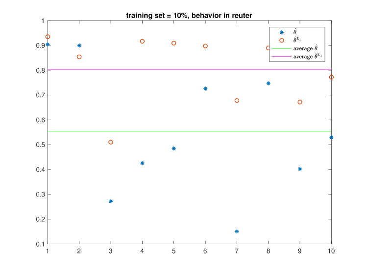
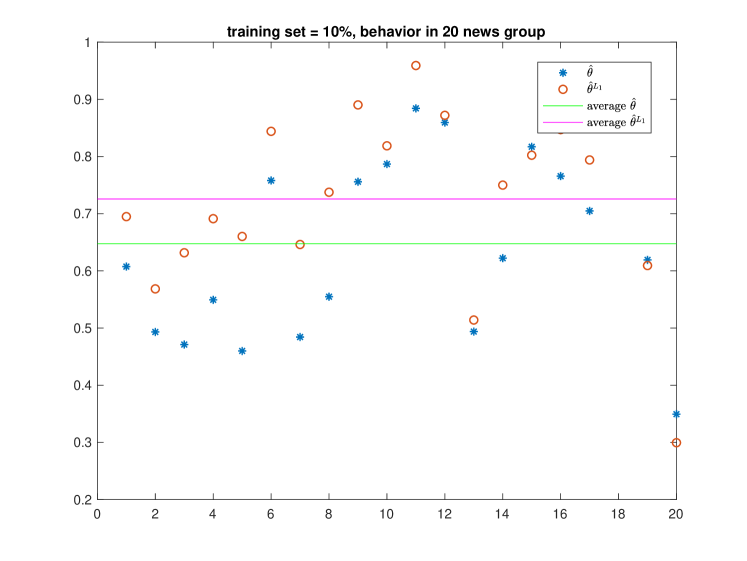
We applied our method on top 10 topics of single labeled documents in Reuters-21578 data[11], and 20 news group data[12]. we compare the result of traditional Naive Bayes estimator (5): $\hat{\theta}_{i_{j}}$and our estimator (11): $\hat{\theta}_{i_{j}}^{L_{1}}$. In this simulation,our correlation factor $t$ is chosen to be $1$ for Figure.1, Figure.2 and Figure.3.

First of all, we run both algorithms on these two sample sets. We know that when sample size becomes large enough, our estimator actually convergences into something else. But when training set is small, our estimator should converge faster. Thus we first take the training size relatively small. See Figure.1 and Figure.1. According to the simulation, we can see our method is more accurate for most of the classes, and more accurate in average.

Figure 1: We take 10 largest groups in Reuter-21578 dataset (a) and 20 news group dataset (b), and take 10% of the data as training set. The y-axis is the accuracy, and the x-axis is the class index.

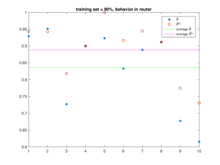
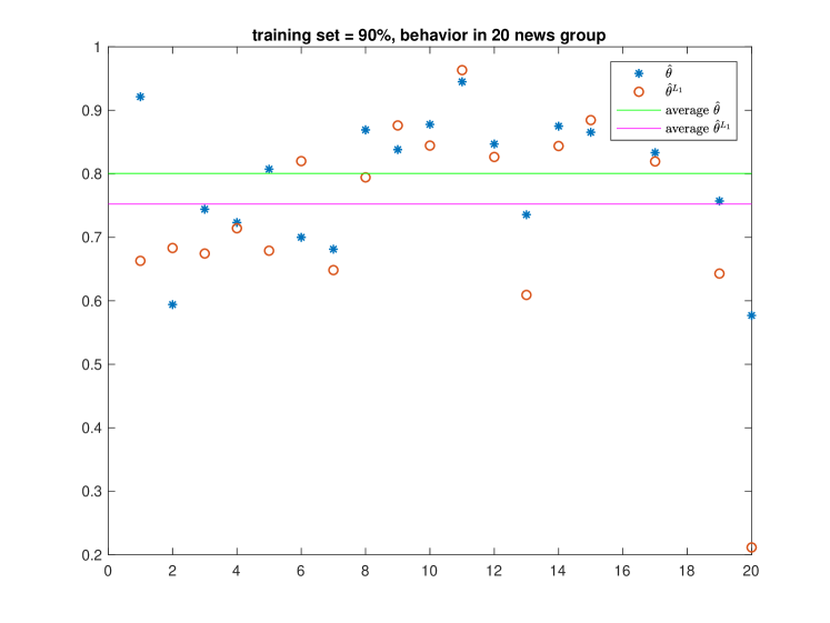
Then we test our estimator $\hat{\theta}^{L_{1}}$ with larger dataset. In our analysis above, we know that as dataset becomes large enough, our estimator converges to something else, so we expect a better result with traditional Naive Bayes estimator. See Figure.2 and Figure.2. According to the simulation, we can see for 20 news group, traditional Naive Bayes performs better than our method, but our method is still more accurate than Naive Bayes in Reuter’s data. The reason might be that we have a huge unbalance dataset in Reuter’s data, 90% of the training set is still not large enough for many classes.

Figure 2: We take 10 largest groups in Reuter-21578 dataset (a) and 20 news group dataset (b), and take 90% of the data as training set. The y-axis is the accuracy, and the x-axis is the class index.

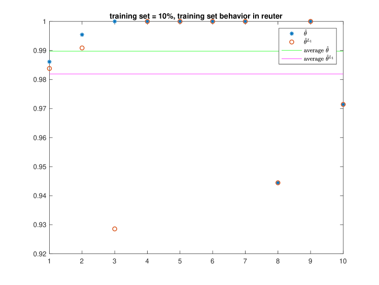
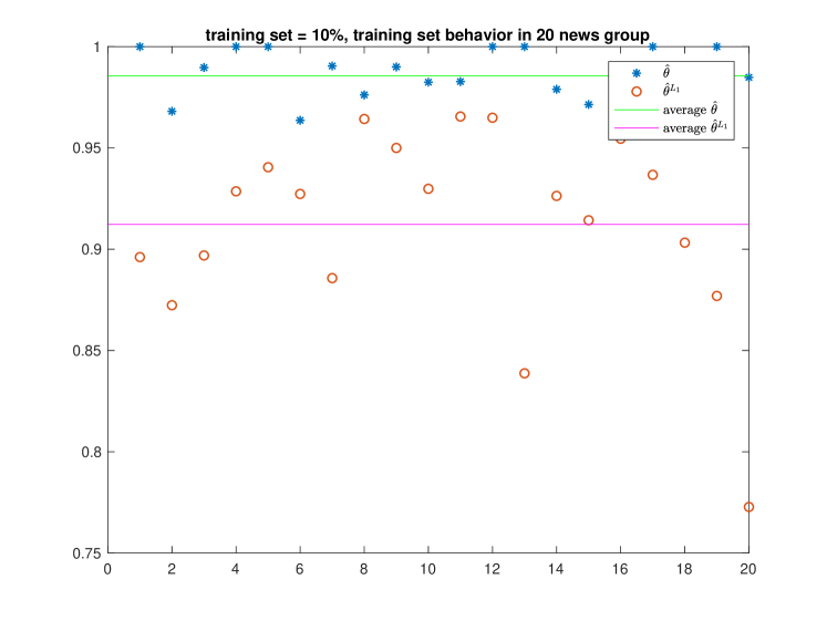
Finally, We apply same training set with training size 10$\%$ and test the accuracy on training set instead of test set. We find traditional Naive Bayes estimator actually achieves better result, which means it might have more over-fitting problems. This might be the reason why our method works better when dataset is not too large: adding the correlation factor $t$ helps us bring some uncertainty in training process, which helps avoid over-fitting. See Figure.3 and Figure.3.

Figure 3: We take 10 largest groups in Reuter-21578 dataset (a), and 20 news group dataset (b), and take 10% of the data as training set. We test the result on training set. The y-axis is the accuracy, and the x-axis is the class index.

V-B Simulation with Different Correlation Factor

In our estimator (11), we need to determine how to choose correlation factor $t$. An idea is to choose $t$ to minimize the variance (12). Taking derivative of (12) with respect to $t$ and setting it to be 0, we find $t$ satisfies:

$$(p_{i}-t-1)\theta_{i_{j}}(1-\theta_{i_{j}})+t\sum_{l=1}^{k}p_{l}\theta_{l_{j}}(1-\theta_{l_{j}})=0,$$

that is:

$$t=\frac{(1-p_{i})\theta_{i_{j}}(1-\theta_{i_{j}})}{[\sum_{l=1}^{k}p_{l}\theta_{l_{j}}(1-\theta_{l_{j}})]-\theta_{i_{j}}(1-\theta_{i_{j}})}$$ (14)

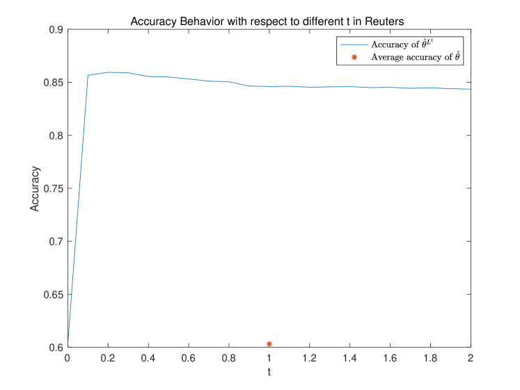
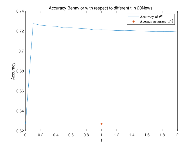
We can see from (14) that our correlation factor $t$ should be less than 1. In our simulation, we notice that when we choose correlation factor to be around 0.1, we get best accuracy for our estimation. See Figure.4 and Figure.4.

Figure 4: We test accuracy behavior with respect to different correlation factors in Reuter-21578 (a) and 20 News group dataset (b). We take 10% of the data as training set. The y-axis is the accuracy and the x-axis is the correlation factor $t$

VI Conclusion

In this paper, we modified the traditional Naive Bayes estimator with a correlation factor to obtain a new estimator, which is biased but with a smaller variance. We applied our estimator in text classification problems, and showed that it works better when training data set is small.

There are several important questions related our estimator:

1. We have a parameter, correlation factor $t$, in our estimator (11). In Section V, we have some simulations when $t=1$, and further show what happened when $t$ ranges from $[0,2]$, but we don’t have theoretical result about how to choose $t$. One important question is how can we choose $t$ in different problems, in each of these problems, can we solve $t$ explicitly?

2. We only test our result in Reuter’s data [11] and 20 news group [12], these datasets are news from newspapers, which means they are highly correlated to each other. Will our estimator still work in other more independent datasets?

3. We can only use our method in single labeled dataset so far, it would be interesting to see if we can extend our result in partial labeled dataset or multi-labeled dataset.

References

• [1] C. Cortes and V. Vapnik, “Support-vector networks,” Machine learning, vol. 20, no. 3, pp. 273–297, 1995.
• [2] T. Joachims, “Text categorization with support vector machines: Learning with many relevant features,” in European conference on machine learning.   Springer, 1998, pp. 137–142.
• [3] N. Friedman, D. Geiger, and M. Goldszmidt, “Bayesian network classifiers,” Machine learning, vol. 29, no. 2-3, pp. 131–163, 1997.
• [4] P. Langley, W. Iba, K. Thompson et al., “An analysis of bayesian classifiers,” in Aaai, vol. 90, 1992, pp. 223–228.
• [5] J. Chen, H. Matzinger, H. Zhai, and M. Zhou, “Centroid estimation based on symmetric kl divergence for multinomial text classification problem,” in 2018 17th IEEE International Conference on Machine Learning and Applications (ICMLA).   IEEE, 2018, pp. 1174–1177.
• [6] D. Tang, B. Qin, and T. Liu, “Document modeling with gated recurrent neural network for sentiment classification,” in Proceedings of the 2015 conference on empirical methods in natural language processing, 2015, pp. 1422–1432.
• [7] P. Liu, X. Qiu, and X. Huang, “Recurrent neural network for text classification with multi-task learning,” arXiv preprint arXiv:1605.05101, 2016.
• [8] R. Albright, “Taming text with the svd,” SAS Institute Inc, 2004.
• [9] T. Hofmann, “Probabilistic latent semantic analysis,” in Proceedings of the Fifteenth conference on Uncertainty in artificial intelligence.   Morgan Kaufmann Publishers Inc., 1999, pp. 289–296.
• [10] D. M. Blei, A. Y. Ng, and M. I. Jordan, “Latent dirichlet allocation,” Journal of machine Learning research, vol. 3, no. Jan, pp. 993–1022, 2003.
• [11] D. D. Lewis, “Reuters-21578.”
• [12] K. Lang, “20 newsgroups data set.” [Online]. Available: http://www.ai.mit.edu/people/jrennie/20Newsgroups/
• [13] V. Koltchinskii and K. Lounici, “Concentration Inequalities and Moment Bounds for Sample Covariance Operators,” arXiv:1405.2468 [math], May 2014, arXiv: 1405.2468. [Online]. Available: http://arxiv.org/abs/1405.2468
• [14] V. Koltchinskii, K. Lounici et al., “Asymptotics and concentration bounds for bilinear forms of spectral projectors of sample covariance,” in Annales de l’Institut Henri Poincaré, Probabilités et Statistiques, vol. 52.   Institut Henri Poincaré, 2016, pp. 1976–2013.
• [15] ——, “Normal approximation and concentration of spectral projectors of sample covariance,” The Annals of Statistics, vol. 45, no. 1, pp. 121–157, 2017.
• [16] K.-M. Schneider, “A new feature selection score for multinomial naive bayes text classification based on kl-divergence,” in Proceedings of the ACL 2004 on Interactive poster and demonstration sessions.   Association for Computational Linguistics, 2004, p. 24.
• [17] J. Ramos et al., “Using tf-idf to determine word relevance in document queries,” in Proceedings of the first instructional conference on machine learning, vol. 242, 2003, pp. 133–142.
• [18] A. McCallum, K. Nigam et al., “A comparison of event models for naive bayes text classification,” in AAAI-98 workshop on learning for text categorization, vol. 752.   Citeseer, 1998, pp. 41–48.
• [19] S. Dumais, J. Platt, D. Heckerman, and M. Sahami, “Inductive learning algorithms and representations for text categorization,” in Proceedings of the seventh international conference on Information and knowledge management.   ACM, 1998, pp. 148–155.
• [20] L. S. Larkey, “Automatic essay grading using text categorization techniques,” in Proceedings of the 21st annual international ACM SIGIR conference on Research and development in information retrieval.   ACM, 1998, pp. 90–95.
• [21] T. Cour, B. Sapp, and B. Taskar, “Learning from partial labels,” Journal of Machine Learning Research, vol. 12, no. May, pp. 1501–1536, 2011.
• [22] X. Li and B. Liu, “Learning to classify texts using positive and unlabeled data,” in IJCAI, vol. 3, 2003, pp. 587–592.
• [23] R. Jin and Z. Ghahramani, “Learning with multiple labels,” in Advances in neural information processing systems, 2003, pp. 921–928.
• [24] M.-L. Zhang and Z.-H. Zhou, “A review on multi-label learning algorithms,” IEEE transactions on knowledge and data engineering, vol. 26, no. 8, pp. 1819–1837, 2014.
• [25] I. Rish et al., “An empirical study of the naive bayes classifier,” in IJCAI 2001 workshop on empirical methods in artificial intelligence, vol. 3.   IBM New York, 2001, pp. 41–46.
• [26] Jeff, “Dimension reduction with pca.” [Online]. Available: https://www.polarmicrobes.org/dimension-reduction-with-pca/