11institutetext: W.  Song 22institutetext: Department of Physics, Hanyang University, Seoul 04763, Korea 33institutetext: Center for Quantum Information, Korea Institute of Science and Technology (KIST), Seoul, 02792, Korea 44institutetext: M. Wieśniak 55institutetext: Institute of Theoretical Physics and Astrophysics, Faculty of Mathematics, Physics and Informatics, University of Gdańsk, 80-308 Gdańsk, Poland 66institutetext: International Centre for Theory of Quantum Technologies, University of Gdańsk, 80-308 Gdańsk, Poland 77institutetext: N. Liu 88institutetext: Institute of Natural Science, Shanghai Jiao Tong University, Shanghai 200240, China 99institutetext: Ministry of Education, Key Laboratory in Scientific and Engineering Computing, Shanghai Jiao Tong University, Shanghai 200240, China 1010institutetext: University of Michigan-Shanghai Jiao Tong University Joint Institute, Shanghai 200240, China 1111institutetext: M. Pawłowski 1212institutetext: International Centre for Theory of Quantum Technologies, University of Gdańsk, 80-308 Gdańsk, Poland 1313institutetext: J. Lee (1313email: hyoung@hanyang.ac.kr) 1414institutetext: Department of Physics, Hanyang University, Seoul 04763, Korea 1515institutetext: J. Kim (1515email: jaewan@kias.re.kr) 1616institutetext: School of Computational Sciences, Korea Institute for Advanced Study, Seoul 02455, Korea 1717institutetext: J. Bang (1717email: jbang@etri.re.kr) 1818institutetext: Electronics and Telecommunications Research Institute, Daejeon 34129, Korea 1919institutetext: Correspondence and requests for materials should be addressed to the last three authors.

Tangible reduction in learning sample complexity with large classical samples and small quantum system

Wooyeong Song    Marcin Wieśniak    Nana Liu    Marcin Pawłowski    Jinhyoung Lee    Jaewan Kim    Jeongho Bang
(Received: date / Accepted: date)
Abstract

Quantum computation requires large classical datasets to be embedded into quantum states in order to exploit quantum parallelism. However, this embedding requires considerable resources in general. It would therefore be desirable to avoid it, if possible, for noisy intermediate-scale quantum (NISQ) implementation. Accordingly, we consider a classical-quantum hybrid architecture, which allows large classical input data, with a relatively small-scale quantum system. This hybrid architecture is used to implement a sampling oracle. It is shown that in the presence of noise in the hybrid oracle, the effects of internal noise can cancel each other out and thereby improve the query success rate. It is also shown that such an immunity of the hybrid oracle to noise directly and tangibly reduces the sample complexity in the framework of computational learning theory. This NISQ-compatible learning advantage is attributed to the oracle’s ability to handle large input features.

Keywords:
Quantum Machine Learning Probably-Approximately-Correct (PAC) Learning Classical-Quantum Hybrid Query Sample Complexity

1 Introduction

Many celebrated quantum algorithms have shown promise for the quantum computational speedup Shor99 ; Grover97 ; Harrow09 . However, apart from requiring considerable computational resources needed for the main calculation, many of them involve high costs for introducing “big” classical data into quantum states, for example, by accessing a useful quantum gadget, called quantum random-access memory (QRAM). An efficient QRAM algorithm, named bucket-brigade algorithm, has been developed Giovannetti08-1 ; Giovannetti08-2 . Nevertheless, despite its promise for usefulness, it has some caveats related to physical resources and its ability to correct errors. This has been argued by S. Aaronson in Ref. Aaronson15 . Thus, it is still unclear whether the bucket-brigade QRAM can be a prototype. This issue is well known in quantum computation and quantum machine learning (QML) (see Ref. Arunachalam15 and Chap. 555 of Ref. Ciliberto2018 for additional details on this issue). Therefore, researchers in the field of quantum computation and/or QML are unlikely to decisively state that tangible quantum (learning) speedups can be achieved with noisy intermediate-scale quantum (NISQ) technologies Preskill2018 ; Arute2019 , when a large superposition of data is required. In this context, it is now highly desirable to show the possibility of achieving NISQ-technology-based speedups, namely, without using excessively large data superposition or, equivalently, without accessing the bucket-brigade QRAM.

Toward this end, one promising approach is to consider a classical-quantum hybrid architecture and identify the optimal interplay between classical and quantum strategies. Such approaches have received increasing attention, an example being the consideration of variational formulations Peruzzo14 ; Mcclean16 ; Khoshaman18 ; Zhu18 ; Havlivcek19 . Here, we devise an intriguing type of hybrid architecture, in which the input data remain classical but a small-scale quantum system is employed. Such an architecture differs from those of other classical-quantum hybridization, however it will render the task suitable for the NISQ implementation without requiring an excessively large superposition of the inputs, or equivalently, the bucket-brigade QRAM Yoo14 ; Lee19 ; Bang19-1 . The motivation and background of this study are similar to those of the recent works in Refs. Dunjko18 ; Harrow2020 .

We apply our hybridization to a classification task, a fundamental problem in computation and machine learning. For this, we employ a classical-quantum hybrid oracle designed on the basis of our main idea and assume that the oracle generates noisy samples due to errors resulting from the use of erroneous (internal) quantum gates. A model with such erroneous gates is often referred to as a noisy query model and is integrated in realistic models Buhrman07 ; Cross15 . We demonstrate both analytically and numerically that our hybrid oracle can exhibit a high probability of success for queries. This advantage is attributed to the high capability of the oracle to explore a wider space of solutions, and it naturally leads to a quantum learning advantage, namely, a reduction in the sample complexity, in a computational learning framework Valiant84 ; Langley95 . Our hybridization architecture is applicable in the relevant context of NISQ machine learning Havlivcek19 .

2 Classification with noisy samples

Classification is a fundamental computational problem that is defined as follows Ambainis04 ; Childs13 ; Arunachalam17 . Consider a Boolean function hsuperscripth^{\star} that maps 𝐱=x1x2xn𝐱subscript𝑥1subscript𝑥2subscript𝑥𝑛\mathbf{x}=x_{1}x_{2}\ldots x_{n} (xj{0,1}subscript𝑥𝑗01x_{j}\in\{0,1\} j=1,,nfor-all𝑗1𝑛\forall j=1,\ldots,n) to h(𝐱){0,1}superscript𝐱01h^{\star}(\mathbf{x})\in\{0,1\} 111Here, we consider a binary classification, i.e., mapping {0,1}n{0,1}superscript01𝑛01\{0,1\}^{n}\to\{0,1\}.. Here, an algorithm (or a learner) can invoke an oracle to prepare a (finite) set of samples; given the inputs 𝐱𝐱\mathbf{x}, the oracle returns the corresponding outputs h(𝐱)superscript𝐱h^{\star}(\mathbf{x}) and generates a set of samples T={(𝐱,h(𝐱))}𝑇𝐱superscript𝐱T=\{(\mathbf{x},h^{\star}(\mathbf{x}))\}. The task is to identify a hypothesis hh close to hsuperscripth^{\star} from among a set, say H𝐻H, of candidates while minimizing the number of invocations of the oracle, or equivalently, the size of samples |T|𝑇\left|T\right|. The oracle can be implemented by using the general form of the Boolean function Gupta06

h(𝐱)=a0a1x1a2x2a3x1x2a2n1x1x2xn,superscript𝐱direct-sumsubscript𝑎0subscript𝑎1subscript𝑥1subscript𝑎2subscript𝑥2subscript𝑎3subscript𝑥1subscript𝑥2subscript𝑎superscript2𝑛1subscript𝑥1subscript𝑥2subscript𝑥𝑛\displaystyle h^{\star}(\mathbf{x})=a_{0}\oplus a_{1}x_{1}\oplus a_{2}x_{2}\oplus a_{3}x_{1}x_{2}\oplus\cdots\oplus a_{2^{n}-1}x_{1}x_{2}\ldots x_{n}, (1)

where ak{0,1}subscript𝑎𝑘01a_{k}\in\{0,1\} (k=0,1,,2n1𝑘01superscript2𝑛1k=0,1,\ldots,2^{n}-1) are known as the Reed-Muller coefficients. In other words, given 𝐱=x1x2xn𝐱subscript𝑥1subscript𝑥2subscript𝑥𝑛\mathbf{x}=x_{1}x_{2}\cdots x_{n}, the oracle outputs, which could be either ideal or noisy. In this study, we are interested in noisy outputs, namely, the case where the oracle provides invalid outputs, resulting in a noisy sample set T~~𝑇\tilde{T}. Note that the classification problem for noisy samples has widely been studied in computational learning theory since real-world data are not clean, which makes the computation much harder Angluin88 ; Angluin94 .

Here, we can introduce a corresponding error model of the generation of T~~𝑇\tilde{T}. For this, each coefficient aksubscript𝑎𝑘a_{k} is changed such that akak1subscript𝑎𝑘direct-sumsubscript𝑎𝑘1a_{k}\to a_{k}\oplus 1 with a certain probability ηk12subscript𝜂𝑘12\eta_{k}\leq\frac{1}{2}, and from the changed coefficients, noisy samples (𝐱,h(𝐱)e)𝐱direct-sumsuperscript𝐱𝑒(\mathbf{x},h^{\star}(\mathbf{x})\oplus e), where e𝑒e is to be 00 (or 111) with probability (say) P(𝐱)𝑃𝐱P(\mathbf{x}) (or 1P(𝐱)1𝑃𝐱1-P(\mathbf{x})), can be obtained. This situation is often referred to as classification error in a noisy query model of computation Bshouty98 . Such a model is useful since Eq. (1) is a general form and each aksubscript𝑎𝑘a_{k} can be realized by a Toffoli gate conditioned by 𝐱𝐱\mathbf{x} channels in a circuit Toffoli80 ; Younes2004 (this is shown later). In this case, the oracle’s invalid outputs are provided by flipping (i.e., 01010\rightleftharpoons 1) the bit signal with probability ηksubscript𝜂𝑘\eta_{k} before or after applying the k𝑘kth Toffoli gate, namely, aksubscript𝑎𝑘a_{k}. This error model can indicate a situation where the probability P(𝐱)𝑃𝐱P(\mathbf{x}) of a successful query decreases as the problem size n𝑛n increases, and it is well suited for determining the effect of noise in complexity-theoretic studies Yoo14 .

3 Classical-quantum hybrid oracle
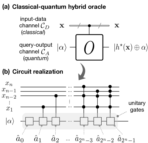
Refer to caption
Figure 1: (a) Schematic of our hybrid oracle. The oracle consists of two different input/output (I/O) channel types, one for input classical data 𝐱=x1x2xn𝐱subscript𝑥1subscript𝑥2subscript𝑥𝑛\mathbf{x}=x_{1}x_{2}\cdots x_{n} (xj{0,1}subscript𝑥𝑗01x_{j}\in\{0,1\} j=1,,nfor-all𝑗1𝑛\forall j=1,\ldots,n), where n𝑛n can be very large, and the other for a single qubit, which produces the query-output states |h(𝐱){0,1}ketsuperscript𝐱01\left|h^{\star}(\mathbf{x})\right>\in\{0,1\}. (b) Circuit realization of the oracle. This oracle applies 2nsuperscript2𝑛2^{n} unitary gates a^k{σ^z,iσ^y}subscript^𝑎𝑘subscript^𝜎𝑧𝑖subscript^𝜎𝑦\hat{a}_{k}\in\{\hat{\sigma}_{z},i\hat{\sigma}_{y}\} (k=0,1,,2n1𝑘01superscript2𝑛1k=0,1,\ldots,2^{n}-1) onto the qubit system, conditioned on the values of the classical bits xjsubscript𝑥𝑗x_{j} in 𝐱𝐱\mathbf{x}. In a fully classical case, these gates are either identity or logical-not. Here, we set α=0𝛼0\alpha=0 for convenience.

In classical studies, the oracle handles classical inputs and outputs. By contrast, (fully) quantum approaches begin by changing classical inputs into the corresponding quantum states, such as 𝐱|𝐱𝐱ket𝐱\mathbf{x}\to\left|\mathbf{x}\right>, and the oracle performs the mapping

𝐱|𝐱,α𝐱|𝐱,h(𝐱)e,subscript𝐱ket𝐱𝛼subscript𝐱ket𝐱direct-sumsuperscript𝐱𝑒\displaystyle\sum_{\mathbf{x}}\left|\mathbf{x},\alpha\right>\to\sum_{\mathbf{x}}\left|\mathbf{x},h^{\star}(\mathbf{x})\oplus e\right>, (2)

in which the quantum parallelism resulting from the superposition of the samples is utilized 222Here we should clarify that such an oracle is employed for data-sampling, which it differs from those employed, for example, in the context of so-called amplitude amplification, where the oracle marks the relative phase on a single data state among superposed ones. In amplitude amplification studies, the primary objective is to reduce the number of iterations of the phase-marking oracle by using other incorporating modules Van1998 .. This oracle enables us to enjoy a quantum computational advantage in a specific situation Arunachalam17 . However, such a process involves considerable cost and can even offset the advantages gained, as described at the beginning of this paper.

In line with our motivation and goal, we thus consider a classical-quantum hybrid oracle that allows classical inputs 𝐱𝐱\mathbf{x} and a small (a single qubit in our case) quantum system for the output (see Fig. 1(a)). More specifically, the oracle performs the mapping

(𝐱,|α)(𝐱,|ψout(𝐱)),𝐱ket𝛼𝐱ketsubscript𝜓out𝐱\displaystyle\left(\mathbf{x},\left|\alpha\right>\right)\to\left(\mathbf{x},\left|\psi_{\text{out}}(\mathbf{x})\right>\right), (3)

where |αket𝛼\left|\alpha\right> is an arbitrary fiducial state and the output state |ψout(𝐱)ketsubscript𝜓out𝐱\left|\psi_{\text{out}}(\mathbf{x})\right> has the form Cross15 ; Bang19-1

|ψout(𝐱)=P(𝐱)|h(𝐱)+Q(𝐱)|h(𝐱)1,ketsubscript𝜓out𝐱𝑃𝐱ketsuperscript𝐱𝑄𝐱ketdirect-sumsuperscript𝐱1\displaystyle\left|\psi_{\text{out}}(\mathbf{x})\right>=\sqrt{P(\mathbf{x})}\left|h^{\star}(\mathbf{x})\right>+\sqrt{Q(\mathbf{x})}\left|h^{\star}(\mathbf{x})\oplus 1\right>, (4)

where Q(𝐱)=1P(𝐱)𝑄𝐱1𝑃𝐱Q(\mathbf{x})=1-P(\mathbf{x}). Then, we can obtain a valid (or invalid) sample with probability P(𝐱)𝑃𝐱P(\mathbf{x}) (or Q(𝐱)𝑄𝐱Q(\mathbf{x})), which is consistent with the error model described above. Note that 𝐱𝐱\mathbf{x} remains unaltered during and after the mapping.

This hybrid oracle can be realized by using the circuit shown in Fig. 1(b). The circuit contains 2nsuperscript2𝑛2^{n} gates acting on the ancilla qubit, namely, the single-qubit gate a^0subscript^𝑎0\hat{a}_{0} and 2n1superscript2𝑛12^{n}-1 of gates a^ksubscript^𝑎𝑘\hat{a}_{k} (k=1,2,,2n1𝑘12superscript2𝑛1k=1,2,\ldots,2^{n}-1) conditioned on the classical bit values x1,x2,,xnsubscript𝑥1subscript𝑥2subscript𝑥𝑛x_{1},x_{2},\ldots,x_{n} in 𝐱𝐱\mathbf{x}. The gates a^ksubscript^𝑎𝑘\hat{a}_{k} are

a^k{σ^z,iσ^y},for allk=0,1,,2n1,formulae-sequencesubscript^𝑎𝑘subscript^𝜎𝑧𝑖subscript^𝜎𝑦for all𝑘01superscript2𝑛1\displaystyle\hat{a}_{k}\in\left\{\hat{\sigma}_{z},i\hat{\sigma}_{y}\right\},~{}\text{for all}~{}k=0,1,\ldots,2^{n}-1, (5)

where σ^xsubscript^𝜎𝑥\hat{\sigma}_{x}, σ^ysubscript^𝜎𝑦\hat{\sigma}_{y}, and σ^zsubscript^𝜎𝑧\hat{\sigma}_{z} are the Pauli operators. Such a circuit realization is consistent with that described in the previous section and Eq. (1). Actually, each coefficient aksubscript𝑎𝑘a_{k} has a corresponding gate operation a^ksubscript^𝑎𝑘\hat{a}_{k}. More specifically, ak=0subscript𝑎𝑘0a_{k}=0 means that a^ksubscript^𝑎𝑘\hat{a}_{k} leaves the bit signal unchanged (identity) and ak=1subscript𝑎𝑘1a_{k}=1 indicates that a^ksubscript^𝑎𝑘\hat{a}_{k} flips the bit signal (logical-not). The oracle is thus characterized by a fixed set of a^ksubscript^𝑎𝑘\hat{a}_{k}’s. The gates a^ksubscript^𝑎𝑘\hat{a}_{k} and their operation are not opened, and the task is to identify all of them.

We can consider an error model consistently where the incorrect oracle answer h(𝐱)1direct-sumsuperscript𝐱1h^{\star}(\mathbf{x})\oplus 1 arises from the systematic errors in the gates a^ksubscript^𝑎𝑘\hat{a}_{k}. More specifically, the error can be described by |ψk(𝐱)|ψk(𝐱)=ϵ^k|ψk(𝐱)ketsubscript𝜓𝑘𝐱ketsuperscriptsubscript𝜓𝑘𝐱subscript^italic-ϵ𝑘ketsubscript𝜓𝑘𝐱\left|\psi_{k}(\mathbf{x})\right>\to\left|\psi_{k}^{\prime}(\mathbf{x})\right>=\hat{\epsilon}_{k}\left|\psi_{k}(\mathbf{x})\right>, where |ψk(𝐱)ketsubscript𝜓𝑘𝐱\left|\psi_{k}(\mathbf{x})\right> is the state passing through the gate a^ksubscript^𝑎𝑘\hat{a}_{k}. Here, ϵ^ksubscript^italic-ϵ𝑘\hat{\epsilon}_{k} is a bit-flip operator defined as ϵ^k=1ηk11^±iηkσ^xsubscript^italic-ϵ𝑘plus-or-minus1subscript𝜂𝑘^11𝑖subscript𝜂𝑘subscript^𝜎𝑥\hat{\epsilon}_{k}=\sqrt{1-\eta_{k}}\hat{1\!\!1}\pm i\sqrt{\eta_{k}}\hat{\sigma}_{x}. In addition, we should consider another type of quantum error, the phase-flip error. This is a challenge for our hybrid oracle because in general, the phase-flip does not occur in classical gates. Thus, the prospect of quantum advantage (to be proved) can be claimed more confidently. The aforementioned error model is realistic, for example, for ion-trap or superconducting qubits, where the systematic errors are caused by imperfect control pulses Debnath16 .

4 Analysis

We now analyze the query success probability PC,Qsubscript𝑃𝐶𝑄P_{C,Q} in Eq. (4). Here, the subscripts Q𝑄Q and C𝐶C refer to when the ancilla system in our hybrid oracle is quantum or classical, respectively. First, let us define a set Ω𝐱={0,l1,l2,,lκ1}subscriptΩ𝐱0subscript𝑙1subscript𝑙2subscript𝑙𝜅1\Omega_{\mathbf{x}}=\{0,l_{1},l_{2},\ldots,l_{\kappa-1}\} whose elements are the indices of the gates a^ksubscript^𝑎𝑘\hat{a}_{k} that are “activated” (i.e., when the corresponding classical control bit xk=1subscript𝑥𝑘1x_{k}=1). The number of activated gates is given by κ=2ω(𝐱)𝜅superscript2𝜔𝐱\kappa=2^{\omega(\mathbf{x})}, where ω(𝐱)𝜔𝐱\omega(\mathbf{x}) denotes the Hamming weight of 𝐱=x1x2xn𝐱subscript𝑥1subscript𝑥2subscript𝑥𝑛\mathbf{x}=x_{1}x_{2}\cdots x_{n}, namely, the number of xjsubscript𝑥𝑗x_{j}’s with a value of 111 for j[1,n]𝑗1𝑛j\in[1,n]. Then, PC,Qsubscript𝑃𝐶𝑄P_{C,Q} can be written in terms of ω𝜔\omega. In the classical case, PC(ω)subscript𝑃𝐶𝜔P_{C}(\omega) can be estimated as

PC(ω)jκ/2(κ2j)(1η¯)2jη¯κ2j12(1+e2ωc),similar-to-or-equalssubscript𝑃𝐶𝜔superscriptsubscript𝑗𝜅2binomial𝜅2𝑗superscript1¯𝜂2𝑗superscript¯𝜂𝜅2𝑗similar-to-or-equals121superscript𝑒superscript2𝜔𝑐\displaystyle P_{C}(\omega)\simeq\sum_{j}^{\kappa/2}{{\kappa}\choose{2j}}\left(1-\overline{\eta}\right)^{2j}\overline{\eta}^{\kappa-2j}\simeq\frac{1}{2}\left(1+e^{-\frac{2^{\omega}}{c}}\right), (6)

where η¯¯𝜂\overline{\eta} is the average error probability given by η¯=1|Ω𝐱|kΩ𝐱ηk¯𝜂1subscriptΩ𝐱subscript𝑘subscriptΩ𝐱subscript𝜂𝑘{\overline{\eta}=\frac{1}{\left|\Omega_{\mathbf{x}}\right|}\sum_{k\in\Omega_{\mathbf{x}}}\eta_{k}}. The variance of the error probability, given by Δη2=1|Ω𝐱|kΩ𝐱ηk2η¯2superscriptsubscriptΔ𝜂21subscriptΩ𝐱subscript𝑘subscriptΩ𝐱superscriptsubscript𝜂𝑘2superscript¯𝜂2{\Delta_{\eta}^{2}=\frac{1}{\left|\Omega_{\mathbf{x}}\right|}\sum_{k\in\Omega_{\mathbf{x}}}\eta_{k}^{2}-\overline{\eta}^{2}}, is assumed to be small. The factor c𝑐c is defined as

c=1ln(12η¯)(2η¯)1,𝑐112¯𝜂similar-to-or-equalssuperscript2¯𝜂1\displaystyle c=-\frac{1}{\ln{(1-2\overline{\eta})}}\simeq({2\overline{\eta}})^{-1}, (7)

and is termed characteristic constant. Here, it is assumed that O(η¯2)0𝑂superscript¯𝜂20O(\overline{\eta}^{2})\to 0. From Eq. (6), c𝑐c can be interpreted as the characteristic number, say κ𝜅\kappa, of steps in the gate operations allowed before the oracle begins to give completely random outputs which cannot be used for learning.

In the case of our hybrid architecture, the success probability PQ(ω)subscript𝑃𝑄𝜔P_{Q}(\omega) is expressed as

PQ(ω)=|h(𝐱)|ϵ^lκ1a^lκ1ϵ^l1a^l1ϵ^0a^0|α|2.subscript𝑃𝑄𝜔superscriptquantum-operator-productsuperscript𝐱subscript^italic-ϵsubscript𝑙𝜅1subscript^𝑎subscript𝑙𝜅1subscript^italic-ϵsubscript𝑙1subscript^𝑎subscript𝑙1subscript^italic-ϵ0subscript^𝑎0𝛼2\displaystyle P_{Q}(\omega)=\left|\left<h^{\star}(\mathbf{x})\right|\hat{\epsilon}_{l_{\kappa-1}}\hat{a}_{l_{\kappa-1}}\cdots\hat{\epsilon}_{l_{1}}\hat{a}_{l_{1}}\hat{\epsilon}_{0}\hat{a}_{0}\left|\alpha\right>\right|^{2}. (8)

Here, using

{σ^x,a^k}+=σ^xa^k+a^kσ^x=0,subscriptsubscript^𝜎𝑥subscript^𝑎𝑘subscript^𝜎𝑥subscript^𝑎𝑘subscript^𝑎𝑘subscript^𝜎𝑥0\displaystyle\{\hat{\sigma}_{x},\hat{a}_{k}\}_{+}=\hat{\sigma}_{x}\hat{a}_{k}+\hat{a}_{k}\hat{\sigma}_{x}=0, (9)

we can show that PQ(ω)subscript𝑃𝑄𝜔P_{Q}(\omega) becomes unity in the limit Δη0subscriptΔ𝜂0\Delta_{\eta}\to 0. Thus, as long as the gate errors are regular, namely, ηk=η¯subscript𝜂𝑘¯𝜂\eta_{k}=\overline{\eta} (kΩ𝐱for-all𝑘subscriptΩ𝐱\forall k\in\Omega_{\mathbf{x}}Cross15 , our hybrid oracle makes no mistakes. Evidently, our gates a^ksubscript^𝑎𝑘\hat{a}_{k} in Eq. (5) satisfy the anticommutation relation in Eq. (9), resulting in the amplitudes associated with gate errors canceling out through destructive interference.

However, it is impractical to realize such a perfect oracle that makes no mistakes, since in a realistic situation, it is difficult to meet the condition Δη=0subscriptΔ𝜂0\Delta_{\eta}=0. Furthermore, we should consider the phase-flip; this is crucial to generate a successful query output since the amplitudes changed by the gate errors would interfere in a disorderly manner because of the phase-flip. In fact, such a feature is often encountered in many physics models, for example, when dealing with localization problems Eleuch17 . Consequently, PQ(ω)subscript𝑃𝑄𝜔P_{Q}(\omega) has a form analogous to that of Eq. (6). The characteristic constant c𝑐c is replaced with an “effective” one ceff(2η¯eff)1similar-to-or-equalssubscript𝑐effsuperscript2subscript¯𝜂eff1c_{\text{eff}}\simeq(2\overline{\eta}_{\text{eff}})^{-1}, where again, O(η¯2)0𝑂superscript¯𝜂20O(\overline{\eta}^{2})\to 0. Here, η¯effsubscript¯𝜂eff\overline{\eta}_{\text{eff}} is defined in terms of the effective average error of the a^ksubscript^𝑎𝑘\hat{a}_{k}’s. Notably, it is considerably smaller than η¯¯𝜂\overline{\eta}, since η¯effsubscript¯𝜂eff\overline{\eta}_{\text{eff}} originates from the errors remaining after destructive interference. Surprisingly, this feature, namely,

η¯effη¯or equivalentlyceffc,subscript¯𝜂eff¯𝜂or equivalentlysubscript𝑐eff𝑐\displaystyle\overline{\eta}_{\text{eff}}\leq\overline{\eta}~{}\text{or equivalently}~{}c_{\text{eff}}\geq c, (10)

does not depend on η¯¯𝜂\overline{\eta} but rather on ΔηsubscriptΔ𝜂\Delta_{\eta}. For a more detailed analysis, see Appendix A.

On the basis of this feature, we show a quantum advantage. We begin with the average Hamming weight ω¯=n2¯𝜔𝑛2\overline{\omega}=\frac{n}{2} for a given number n𝑛n of input bit strings. Then, on average, our hybrid oracle is useful up to the input bit-string length n=2log2ceff𝑛2subscript2subscript𝑐effn=2\log_{2}{c_{\text{eff}}}, while n=2log2c𝑛2subscript2𝑐n=2\log_{2}{c} is the upper limit in the purely classical case. Hence, if ceffcsubscript𝑐eff𝑐c_{\text{eff}}\geq c, our hybrid oracle can be useful for larger bit-string inputs; this condition also implies the expansion of the space of legitimate samples that can be explored by the erroneous gates, which ranges from O(e(2η¯)2ln2)𝑂superscript𝑒superscript2¯𝜂22O(e^{\left({2\overline{\eta}}\right)^{-2}\ln{2}}) to O(eγ2(2η¯)2ln2)𝑂superscript𝑒superscript𝛾2superscript2¯𝜂22O(e^{\gamma^{2}\left({2\overline{\eta}}\right)^{-2}\ln{2}}), where γ=ceffc𝛾subscript𝑐eff𝑐\gamma=\frac{c_{\text{eff}}}{c} is larger than 111.

In addition to our theoretical analysis, we present numerical simulations in which PC,Q(ω)subscript𝑃𝐶𝑄𝜔P_{C,Q}(\omega) are evaluated by counting a large number (105similar-to-or-equalsabsentsuperscript105\simeq 10^{5}) of queries for each given number of ω(𝐱)𝜔𝐱\omega(\mathbf{x}). Here, the identified data of PC,Q(ω)subscript𝑃𝐶𝑄𝜔P_{C,Q}(\omega) are averaged over the trials (103similar-to-or-equalsabsentsuperscript103\simeq 10^{3}) again. To simulate a more realistic scenario, it is assumed that ηksubscript𝜂𝑘\eta_{k}’s are drawn from a normal distribution 𝒩(η¯,Δη)𝒩¯𝜂subscriptΔ𝜂{\cal N}(\overline{\eta},\Delta_{\eta}). We also assume that the ancilla qubit undergoes the phase-flip errors on the gates a^ksubscript^𝑎𝑘\hat{a}_{k} with probability χk12subscript𝜒𝑘12\chi_{k}\leq\frac{1}{2}, drawn from 𝒩(χ¯,Δχ)𝒩¯𝜒subscriptΔ𝜒{\cal N}(\overline{\chi},\Delta_{\chi}). The simulation results confirm our theoretical analysis, allowing us to determine ceffsubscript𝑐effc_{\text{eff}} and γ𝛾\gamma for a given noise level. For example, when η¯=103¯𝜂superscript103\overline{\eta}=10^{-3} with Δη=5%ofη¯subscriptΔ𝜂percent5of¯𝜂\Delta_{\eta}=5\%~{}\text{of}~{}\overline{\eta}, our hybrid oracle would be applicable up to n27.23similar-to-or-equals𝑛27.23n\simeq 27.23 even in the presence of a phase-flip of χ¯=102¯𝜒superscript102\overline{\chi}=10^{-2}, whereas n17.93similar-to-or-equals𝑛17.93n\simeq 17.93 would be the limit in the purely classical case. Equivalently, the hybrid oracle can cover a space up to about O(e1.09×108)𝑂superscript𝑒1.09superscript108O(e^{1.09\times 10^{8}}) scale, which is considerably larger than the space, about O(e1.73×105)𝑂superscript𝑒1.73superscript105O(e^{1.73\times 10^{5}}) scale, allowed in the classical case. The determined ceffsubscript𝑐effc_{\text{eff}} and γ𝛾\gamma values are listed in Table 1. For details on the methods and results of the numerical analysis, see Appendix B.

      χ¯¯𝜒\overline{\chi}       ceffsubscript𝑐effc_{\text{eff}} (cf., c=0.5×10³𝑐0.5superscript103c=0.5\times 10^{3})       γ=ceffc𝛾subscript𝑐eff𝑐\gamma=\frac{c_{\text{eff}}}{c}
      no phase-flip       0.5×106.230.5superscript106.230.5\times 10^{6.23}       103.23superscript103.2310^{3.23}
      104superscript10410^{-4}       0.5×106.010.5superscript106.010.5\times 10^{6.01}       103.01superscript103.0110^{3.01}
      103superscript10310^{-3}       0.5×105.340.5superscript105.340.5\times 10^{5.34}       102.34superscript102.3410^{2.34}
      102superscript10210^{-2}       0.5×104.400.5superscript104.400.5\times 10^{4.40}       101.40superscript101.4010^{1.40}
Table 1: Values of ceffsubscript𝑐effc_{\text{eff}} and γ𝛾\gamma are listed for several cases: χ¯=0¯𝜒0\overline{\chi}=0, 104superscript10410^{-4}, 103superscript10310^{-3}, and 102superscript10210^{-2}. Here, η¯¯𝜂\overline{\eta} is assumed to be 103superscript10310^{-3} and Δη=0.05η¯subscriptΔ𝜂0.05¯𝜂\Delta_{\eta}=0.05\overline{\eta}.

5 Reduction of sample complexity

The quantum advantage described above can be applied to a computational model of learning, the so-called PAC learning model. In this model, a finite set of hsuperscripth^{\star}, say Hsuperscript𝐻H^{\star}, is said to be (ϵ,δ)italic-ϵ𝛿(\epsilon,\delta)-PAC learnable and we call the learner (or learning algorithm employed) (ϵ,δ)italic-ϵ𝛿(\epsilon,\delta)-PAC learner, if P[E(h,h)ϵ]1δ𝑃delimited-[]𝐸superscriptitalic-ϵ1𝛿P[E(h,h^{\star})\leq\epsilon]\geq 1-\delta is satisfied for hHsuperscriptsuperscript𝐻h^{\star}\in H^{\star}. Here, E(h,h)𝐸superscriptE(h,h^{\star}) denotes an arbitrary error function that indicates how hh and hsuperscripth^{\star} are different. Borrowing terms from sampling theory in statistics, ϵitalic-ϵ\epsilon and 1δ1𝛿1-\delta are defined in terms of the accuracy and confidence, respectively. One beauty of PAC learning is that for any hHsuperscriptsuperscript𝐻h^{\star}\in H^{\star}, if a learner is allowed to use a finite size, say Mb(ϵ,δ)subscript𝑀𝑏italic-ϵ𝛿M_{b}(\epsilon,\delta), of samples, then the learner can be a (ϵ,δ)italic-ϵ𝛿(\epsilon,\delta)-PAC learner; in other words, we can know whether Hsuperscript𝐻H^{\star} is learnable in terms of the required samples, independent of the learning algorithm used. Usually, Mb(ϵ,δ)subscript𝑀𝑏italic-ϵ𝛿M_{b}(\epsilon,\delta) is referred to as sample complexity. For a given set of noisy samples T~={(𝐱,m)}~𝑇𝐱𝑚\tilde{T}=\{(\mathbf{x},m)\} where m𝑚m is either h(𝐱)superscript𝐱h^{\star}(\mathbf{x}) or h(𝐱)1direct-sumsuperscript𝐱1h^{\star}(\mathbf{x})\oplus 1, it is known that Mb(ϵ,δ)subscript𝑀𝑏italic-ϵ𝛿M_{b}(\epsilon,\delta) is at most 333The determination of its optimal (i.e., necessary and sufficient) condition is central and long-standing interest in computational learning theory, but this aspect is outside the scope of our study Hanneke2016 .

2ϵ2(12ξ)2ln(2|H|δ),2superscriptitalic-ϵ2superscript12𝜉22𝐻𝛿\displaystyle\frac{2}{\epsilon^{2}(1-2\xi)^{2}}\ln{\left(\frac{2\left|H\right|}{\delta}\right)}, (11)

where ξ𝜉\xi is the imperfection of the oracle, that is, the probability ξ𝜉\xi that the oracle provides an incorrect output. For more details about PAC learning, see Refs. Valiant84 ; Angluin94 .

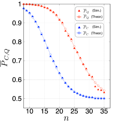
Our previous analysis on the improvement of the query success rate can be extended to the reduction of sample complexity by letting ξ=1P¯Q(n)𝜉1subscript¯𝑃𝑄𝑛\xi=1-\overline{P}_{Q}(n), where P¯Q(n)subscript¯𝑃𝑄𝑛\overline{P}_{Q}(n) is the average query success probability given by P¯Q(n)=12nω=0n(nω)PQ(ω)subscript¯𝑃𝑄𝑛1superscript2𝑛superscriptsubscript𝜔0𝑛binomial𝑛𝜔subscript𝑃𝑄𝜔\overline{P}_{Q}(n)=\frac{1}{2^{n}}\sum_{\omega=0}^{n}{{n}\choose{\omega}}P_{Q}(\omega). Note that P¯Q(n)subscript¯𝑃𝑄𝑛\overline{P}_{Q}(n) would decrease as the number of gates (i.e., 2nsuperscript2𝑛2^{n}) increases, indicating that the oracle’s reliability rapidly worsens as the problem size n𝑛n increases. This is reasonable and shows that the error model is well suited for realistic situations. Here, we introduce the quantity

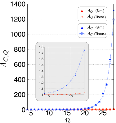
AQ=1(2P¯Q(n)1)2=[j=0(1)jj!(1γc)j(2j+12)n]2,subscript𝐴𝑄1superscript2subscript¯𝑃𝑄𝑛12superscriptdelimited-[]superscriptsubscript𝑗0superscript1𝑗𝑗superscript1𝛾𝑐𝑗superscriptsuperscript2𝑗12𝑛2\displaystyle A_{Q}=\frac{1}{\left(2\overline{P}_{Q}(n)-1\right)^{2}}=\left[\sum_{j=0}^{\infty}\frac{(-1)^{j}}{j!}\left(\frac{1}{\gamma c}\right)^{j}\left(\frac{2^{j}+1}{2}\right)^{n}\right]^{-2}, (12)

which is consistently proportional to the sample complexity consistently but does not depend on ϵitalic-ϵ\epsilon, δ𝛿\delta, and |H|𝐻\left|H\right|. Subsequently, for the sake of comparison, we also consider the case where a purely classical oracle is employed; in this case, the classical counterpart to AQsubscript𝐴𝑄A_{Q} is ACsubscript𝐴𝐶A_{C}, which is defined using P¯C(n)=12nω=0n(nω)PC(ω)subscript¯𝑃𝐶𝑛1superscript2𝑛superscriptsubscript𝜔0𝑛binomial𝑛𝜔subscript𝑃𝐶𝜔\overline{P}_{C}(n)=\frac{1}{2^{n}}\sum_{\omega=0}^{n}{{n}\choose{\omega}}P_{C}(\omega) instead of P¯Q(n)subscript¯𝑃𝑄𝑛\overline{P}_{Q}(n). Then, we can show the reduction of the sample complexity from Eq. (10) and Eq. (29) for AQACsubscript𝐴𝑄subscript𝐴𝐶A_{Q}\leq A_{C}.

This result tells us that for a large n𝑛n, our hybrid oracle allows us to define a (ϵitalic-ϵ\epsilon, δ𝛿\delta)-PAC learner, whereas a fully-classical oracle cannot. What is remarkable is that the sample complexity reduction is achieved with classical samples without the need to embed them into quantum states, unlike other classical-quantum hybrid schemes. Nevertheless, we note that if n𝑛n is too large (roughly, when n2log2γcmuch-greater-than𝑛2subscript2𝛾𝑐n\gg 2\log_{2}{\gamma c}), it is also impractical to define a legitimate PAC learner, even with the quantum learning advantage gained.
Refer to caption
Refer to caption
Figure 2: Numerical plots of P¯C,Qsubscript¯𝑃𝐶𝑄\bar{P}_{C,Q} (left) and AC,Qsubscript𝐴𝐶𝑄A_{C,Q} (right) with respect to n𝑛n. Here, we have used η¯=103¯𝜂superscript103\overline{\eta}=10^{-3} with Δη=0.05η¯subscriptΔ𝜂0.05¯𝜂\Delta_{\eta}=0.05\overline{\eta} and χ¯=102¯𝜒superscript102\overline{\chi}=10^{-2}. Theoretical values are also presented for comparison. Refer to the main text for a detailed description.

To confirm this feature, we perform numerical simulations. P¯C,Q(n)subscript¯𝑃𝐶𝑄𝑛\overline{P}_{C,Q}(n) are evaluated by repeating trials for randomly sampled inputs, with each bit xjsubscript𝑥𝑗x_{j} (j=1,2,,n𝑗12𝑛j=1,2,\ldots,n) in 𝐱𝐱\mathbf{x} being either 00 or 111 with probability 1212\frac{1}{2}, and we examine the range n=8𝑛8n=8 to n=35𝑛35n=35. In these simulations, we assume η¯=103¯𝜂superscript103\overline{\eta}=10^{-3} with Δη=0.05η¯subscriptΔ𝜂0.05¯𝜂\Delta_{\eta}=0.05\overline{\eta} and χ¯=102¯𝜒superscript102\overline{\chi}=10^{-2} with Δχ=0.1χ¯subscriptΔ𝜒0.1¯𝜒\Delta_{\chi}=0.1\overline{\chi}. In Fig. 2, we plot the dependence of P¯C,Qsubscript¯𝑃𝐶𝑄\overline{P}_{C,Q} and AC,Qsubscript𝐴𝐶𝑄A_{C,Q} on n𝑛n. These results agree well with our theoretical predictions. Detailed descriptions of the method and analysis are provided in Appendix C.

6 Summary and remarks

We have studied how a tangible quantum advantage can be achieved on the basis of a classical-quantum hybrid architecture distinct from other existing ones. Our approach is appealing, since the proposed hybridization architecture allows classical input data, without requiring (big) classical data to be embedded into a largely superposed quantum state, for example, by implementing QRAM. Instead, the quantum advantage is achieved with a small-sized quantum system (only a single-qubit is required in our case). We applied this approach to a binary classification problem and found that the oracle designed based on our main idea of classical-quantum hybridization, can improve the query success rate. This advantageous feature was attributed to the cancelation of the quantum amplitudes associated with the oracle’s internal gate errors. Such (say) immunity could lead to a reduction of sample complexity in the PAC learning, facilitating the exploration of a large candidate space with noisy classical samples.

Of the two recent research directions in quantum machine learning—those seeking very strong complexity-theoretic evidence of quantum superiority to be realized in a full-scale quantum computer versus providing prospects for tangible quantum advantages which can be realized with NISQ technologies—our work pertains to the latter. We believe that the presented results are realizable and have potential to facilitate the development of an innovative classical-quantum hybrid technologies.

Acknowledgements.
W.S., N.L., and J.B. are grateful to Gahyun Choi and Yonuk Chong for the valuable discussions on superconducting-qubit experiments. W.S., J.L., and J.B. acknowledge the financial support of the National Research Foundation of Korea (NRF) grants (No. 2019R1A2C2005504, No. NRF-2019M3E4A1079666, and No. 2021M3E4A1038213), funded by the MSIP (Ministry of Science, ICT and Future Planning) of the Korea government. J.B. also acknowledge the support of the Institute of Information and Communications Technology Planning and Evaluation grant funded by the Korea government (Grant No. 2020-0-00890). W.S. and J.B. acknowledge the research project on developing quantum machine learning and quantum algorithm (No. 2018-104) by the ETRI affiliated research institute. W.S. acknowledge the KIST research program (2E31021). N. L. acknowledges funding from the Shanghai Pujiang Talent Grant (no. 20PJ1408400) and the NSFC International Young Scientists Project (no. 12050410230). N. L. is also supported by the Innovation Program of the Shanghai Municipal Education Commission (no. 2021-01-07-00-02-E00087), the Shanghai Municipal Science and Technology Major Project (2021SHZDZX0102) and the Natural Science Foundation of Shanghai grant 21ZR1431000. M.W. and M.P. acknowledge the ICTQT IRAP project of FNP (Contract No. 2018/MAB/5), financed by structural funds of EU. M.P. was supported under FNP grant First Team/2016-1/5. J.K. was supported in part by KIAS Advanced Research Program (No. CG014604). J.B. was supported by a KIAS Individual Grant (No. CG061003).

Appendix A: Detailed calculations of PQ(ω)subscript𝑃𝑄𝜔P_{Q}(\omega)

Refer to caption
Refer to caption
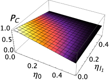
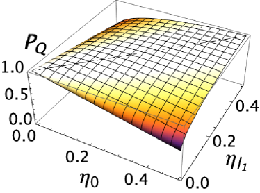
Figure 3: 3D graphs of PCsubscript𝑃𝐶P_{C} (left) and PQsubscript𝑃𝑄P_{Q} (right) with respect to η0subscript𝜂0\eta_{0} and ηl1subscript𝜂subscript𝑙1\eta_{l_{1}} for ω=1𝜔1\omega=1. The advantage defined in Eq. (19) is observed; PQsubscript𝑃𝑄P_{Q} is always larger than PCsubscript𝑃𝐶P_{C}. Here, the most remarkable feature is that our hybrid oracle always yields correct results when PQ=1subscript𝑃𝑄1P_{Q}=1 provided that η0=ηl1subscript𝜂0subscript𝜂subscript𝑙1\eta_{0}=\eta_{l_{1}}.

Here, we present the procedure to calculate PQ(ω)subscript𝑃𝑄𝜔P_{Q}(\omega) in Eq. (6) of the main manuscript. We start by analyzing the simple case, i.e., of ω=1𝜔1\omega=1. In particular, we consider an input 𝐱=x1x2xn𝐱subscript𝑥1subscript𝑥2subscript𝑥𝑛\mathbf{x}=x_{1}x_{2}\cdots x_{n} satisfying xl1=1subscript𝑥subscript𝑙11x_{l_{1}}=1 for arbitrary l1[1,n]subscript𝑙11𝑛l_{1}\in[1,n] and xj=0subscript𝑥𝑗0x_{j}=0 for all jl1𝑗subscript𝑙1j\neq l_{1}. Subsequently, only two gates a^0subscript^𝑎0\hat{a}_{0} and a^l1subscript^𝑎subscript𝑙1\hat{a}_{l_{1}} are activated with Ω𝐱={0,l1}subscriptΩ𝐱0subscript𝑙1\Omega_{\mathbf{x}}=\{0,l_{1}\}. In a purely classical query, PC(ω=1)subscript𝑃𝐶𝜔1P_{C}(\omega=1) is given as

PC(ω=1)=(1ηl1)(1η0)+ηl1η0,subscript𝑃𝐶𝜔11subscript𝜂subscript𝑙11subscript𝜂0subscript𝜂subscript𝑙1subscript𝜂0\displaystyle P_{C}(\omega=1)=\left(1-\eta_{l_{1}}\right)\left(1-\eta_{0}\right)+\eta_{l_{1}}\eta_{0}, (13)

where ηksubscript𝜂𝑘\eta_{k} is the probability that a bit-flip error will occur at a^ksubscript^𝑎𝑘\hat{a}_{k} (k{0,l1}𝑘0subscript𝑙1k\in\{0,l_{1}\}). Meanwhile, PQ(ω=1)subscript𝑃𝑄𝜔1P_{Q}(\omega=1) is calculated as below:

PQ(ω=1)subscript𝑃𝑄𝜔1\displaystyle P_{Q}(\omega=1) =\displaystyle= |h(𝐱)|ϵ^l1a^l1ϵ^0a^0|α|2,superscriptquantum-operator-productsuperscript𝐱subscript^italic-ϵsubscript𝑙1subscript^𝑎subscript𝑙1subscript^italic-ϵ0subscript^𝑎0𝛼2\displaystyle\left|\left<h^{\star}(\mathbf{x})\right|{\hat{\epsilon}_{l_{1}}\hat{a}_{l_{1}}\hat{\epsilon}_{0}\hat{a}_{0}}\left|\alpha\right>\right|^{2},
=\displaystyle= |h(𝐱)|(1ηl111^±iηl1σ^x)a^l1(1η011^±iη0σ^x)a^0|α|2,superscriptquantum-operator-productsuperscript𝐱plus-or-minus1subscript𝜂subscript𝑙1^11𝑖subscript𝜂subscript𝑙1subscript^𝜎𝑥subscript^𝑎subscript𝑙1plus-or-minus1subscript𝜂0^11𝑖subscript𝜂0subscript^𝜎𝑥subscript^𝑎0𝛼2\displaystyle\left|\left<h^{\star}(\mathbf{x})\right|\left(\sqrt{1-\eta_{l_{1}}}\hat{1\!\!1}\pm i\sqrt{\eta_{l_{1}}}\hat{\sigma}_{x}\right)\hat{a}_{l_{1}}\left(\sqrt{1-\eta_{0}}\hat{1\!\!1}\pm i\sqrt{\eta_{0}}\hat{\sigma}_{x}\right)\hat{a}_{0}\left|\alpha\right>\right|^{2},
=\displaystyle= |1ηl11η0h(𝐱)|a^l1a^0|α±i1ηl1η0h(𝐱)|a^l1σ^xa^0|α\displaystyle\left|\sqrt{1-\eta_{l_{1}}}\sqrt{1-\eta_{0}}\left<h^{\star}(\mathbf{x})\right|\hat{a}_{l_{1}}\hat{a}_{0}\left|\alpha\right>\pm i\sqrt{1-\eta_{l_{1}}}\sqrt{\eta_{0}}\left<h^{\star}(\mathbf{x})\right|\hat{a}_{l_{1}}\hat{\sigma}_{x}\hat{a}_{0}\left|\alpha\right>\right.
±iηl11η0h(𝐱)|σ^xa^l1a^0|αηl1η0h(𝐱)|σ^xa^l1σ^xa^0|α|2,\displaystyle\left.\pm i\sqrt{\eta_{l_{1}}}\sqrt{1-\eta_{0}}\left<h^{\star}(\mathbf{x})\right|\hat{\sigma}_{x}\hat{a}_{l_{1}}\hat{a}_{0}\left|\alpha\right>-\sqrt{\eta_{l_{1}}}\sqrt{\eta_{0}}\left<h^{\star}(\mathbf{x})\right|\hat{\sigma}_{x}\hat{a}_{l_{1}}\hat{\sigma}_{x}\hat{a}_{0}\left|\alpha\right>\right|^{2},

where ϵ^k=1ηk11^±iηkσ^xsubscript^italic-ϵ𝑘plus-or-minus1subscript𝜂𝑘^11𝑖subscript𝜂𝑘subscript^𝜎𝑥\hat{\epsilon}_{k}=\sqrt{1-\eta_{k}}\hat{1\!\!1}\pm i\sqrt{\eta_{k}}\hat{\sigma}_{x} is the error operation, defined in the main manuscript. Using the properties in Eq. (7) of the main manuscript, i.e., σ^xa^k=a^kσ^xsubscript^𝜎𝑥subscript^𝑎𝑘subscript^𝑎𝑘subscript^𝜎𝑥\hat{\sigma}_{x}\hat{a}_{k}=-\hat{a}_{k}\hat{\sigma}_{x} and h(𝐱)|a^l1a^0|α=1quantum-operator-productsuperscript𝐱subscript^𝑎subscript𝑙1subscript^𝑎0𝛼1\left<h^{\star}(\mathbf{x})\right|\hat{a}_{l_{1}}\hat{a}_{0}\left|\alpha\right>=1, we can evaluate the following:

{h(𝐱)|a^l1σ^xa^0|α=h(𝐱)|a^l1a^0σ^x|α=0,h(𝐱)|σ^xa^l1a^0|α=h(𝐱)|a^l1a^0σ^x|α=0,h(𝐱)|σ^xa^l1σ^xa^0|α=h(𝐱)|a^l1a^0|α=1.casesquantum-operator-productsuperscript𝐱subscript^𝑎subscript𝑙1subscript^𝜎𝑥subscript^𝑎0𝛼quantum-operator-productsuperscript𝐱subscript^𝑎subscript𝑙1subscript^𝑎0subscript^𝜎𝑥𝛼0quantum-operator-productsuperscript𝐱subscript^𝜎𝑥subscript^𝑎subscript𝑙1subscript^𝑎0𝛼quantum-operator-productsuperscript𝐱subscript^𝑎subscript𝑙1subscript^𝑎0subscript^𝜎𝑥𝛼0quantum-operator-productsuperscript𝐱subscript^𝜎𝑥subscript^𝑎subscript𝑙1subscript^𝜎𝑥subscript^𝑎0𝛼quantum-operator-productsuperscript𝐱subscript^𝑎subscript𝑙1subscript^𝑎0𝛼1\displaystyle\left\{\begin{array}[]{l}\left<h^{\star}(\mathbf{x})\right|\hat{a}_{l_{1}}\hat{\sigma}_{x}\hat{a}_{0}\left|\alpha\right>=-\left<h^{\star}(\mathbf{x})\right|\hat{a}_{l_{1}}\hat{a}_{0}\hat{\sigma}_{x}\left|\alpha\right>=0,\\ \left<h^{\star}(\mathbf{x})\right|\hat{\sigma}_{x}\hat{a}_{l_{1}}\hat{a}_{0}\left|\alpha\right>=\left<h^{\star}(\mathbf{x})\right|\hat{a}_{l_{1}}\hat{a}_{0}\hat{\sigma}_{x}\left|\alpha\right>=0,\\ \left<h^{\star}(\mathbf{x})\right|\hat{\sigma}_{x}\hat{a}_{l_{1}}\hat{\sigma}_{x}\hat{a}_{0}\left|\alpha\right>=-\left<h^{\star}(\mathbf{x})\right|\hat{a}_{l_{1}}\hat{a}_{0}\left|\alpha\right>=-1.\end{array}\right. (18)

Subsequently, using Eq. (18), we can obtain

PQ(ω=1)PC(ω=1)=Γ0,l1,subscript𝑃𝑄𝜔1subscript𝑃𝐶𝜔1subscriptΓ0subscript𝑙1\displaystyle P_{Q}(\omega=1)-P_{C}(\omega=1)=\Gamma_{0,l_{1}}, (19)

where

Γ0,l1=21ηl11η0ηl1η00.subscriptΓ0subscript𝑙121subscript𝜂subscript𝑙11subscript𝜂0subscript𝜂subscript𝑙1subscript𝜂00\displaystyle\Gamma_{0,l_{1}}=2\sqrt{1-\eta_{l_{1}}}\sqrt{1-\eta_{0}}\sqrt{\eta_{l_{1}}}\sqrt{\eta_{0}}\geq 0. (20)

This factor Γ0,l1subscriptΓ0subscript𝑙1\Gamma_{0,l_{1}} is from quantum superposition and clearly indicates the enhancement of the success probability with the condition Γ0,l10subscriptΓ0subscript𝑙10\Gamma_{0,l_{1}}\geq 0. In Fig. 3, we depict the graphs of PC,Qsubscript𝑃𝐶𝑄P_{C,Q} with respect to η0subscript𝜂0\eta_{0} and ηl1subscript𝜂subscript𝑙1\eta_{l_{1}}. It is noteworthy that our hybrid oracle always yields correct results, i.e., PQ=1subscript𝑃𝑄1P_{Q}=1, provided that ηl1=η0subscript𝜂subscript𝑙1subscript𝜂0\eta_{l_{1}}=\eta_{0}, even though ηl1subscript𝜂subscript𝑙1\eta_{l_{1}} and η0subscript𝜂0\eta_{0} are large. This is the most remarkable feature in our classical–quantum hybrid query.

Subsequently, we consider the case of ω=2𝜔2\omega=2, where a set of four gates, a^0subscript^𝑎0\hat{a}_{0}, a^l1subscript^𝑎subscript𝑙1\hat{a}_{l_{1}}, a^l2subscript^𝑎subscript𝑙2\hat{a}_{l_{2}}, and a^l3subscript^𝑎subscript𝑙3\hat{a}_{l_{3}}, are to be activated with Ω𝐱={0,l1,l2,l3}subscriptΩ𝐱0subscript𝑙1subscript𝑙2subscript𝑙3\Omega_{\mathbf{x}}=\{0,l_{1},l_{2},l_{3}\}. We subsequently calculate PQ(ω=2)subscript𝑃𝑄𝜔2P_{Q}(\omega=2) as follows:

PQ(ω=2)=|h(𝐱)|ϵ^l3a^l3ϵ^l2a^l2ϵ^l1a^l1ϵ^0a^0|α|2.subscript𝑃𝑄𝜔2superscriptquantum-operator-productsuperscript𝐱subscript^italic-ϵsubscript𝑙3subscript^𝑎subscript𝑙3subscript^italic-ϵsubscript𝑙2subscript^𝑎subscript𝑙2subscript^italic-ϵsubscript𝑙1subscript^𝑎subscript𝑙1subscript^italic-ϵ0subscript^𝑎0𝛼2\displaystyle P_{Q}(\omega=2)=\left|\left<h^{\star}(\mathbf{x})\right|\hat{\epsilon}_{l_{3}}\hat{a}_{l_{3}}\hat{\epsilon}_{l_{2}}\hat{a}_{l_{2}}\hat{\epsilon}_{l_{1}}\hat{a}_{l_{1}}\hat{\epsilon}_{0}\hat{a}_{0}\left|\alpha\right>\right|^{2}. (21)

To proceed with the calculation, we introduce an identity 11^β,β=|ββ|+|ββ|subscript^11𝛽superscript𝛽perpendicular-toket𝛽bra𝛽ketsuperscript𝛽perpendicular-tobrasuperscript𝛽perpendicular-to\hat{1\!\!1}_{\beta,\beta^{\perp}}=\left|\beta\right>\left<\beta\right|+\left|\beta^{\perp}\right>\left<\beta^{\perp}\right|, where the state |βket𝛽\left|\beta\right> (β{0,1}𝛽01\beta\in\{0,1\}) is defined with the following properties:

|h(𝐱)|a^l3a^l2|β|2=1and|β|a^l1a^0|α|2=1.superscriptquantum-operator-productsuperscript𝐱subscript^𝑎subscript𝑙3subscript^𝑎subscript𝑙2𝛽21andsuperscriptquantum-operator-product𝛽subscript^𝑎subscript𝑙1subscript^𝑎0𝛼21\displaystyle\left|\left<h^{\star}(\mathbf{x})\right|\hat{a}_{l_{3}}\hat{a}_{l_{2}}\left|\beta\right>\right|^{2}=1~{}\text{and}~{}\left|\left<\beta\right|\hat{a}_{l_{1}}\hat{a}_{0}\left|\alpha\right>\right|^{2}=1. (22)

Using a mathematical method of substituting the identity 11^β,βsubscript^11𝛽superscript𝛽perpendicular-to\hat{1\!\!1}_{\beta,\beta^{\perp}} between ϵ^l3a^l3ϵ^l2a^l2subscript^italic-ϵsubscript𝑙3subscript^𝑎subscript𝑙3subscript^italic-ϵsubscript𝑙2subscript^𝑎subscript𝑙2\hat{\epsilon}_{l_{3}}\hat{a}_{l_{3}}\hat{\epsilon}_{l_{2}}\hat{a}_{l_{2}} and ϵ^l1a^l1ϵ^0a^0subscript^italic-ϵsubscript𝑙1subscript^𝑎subscript𝑙1subscript^italic-ϵ0subscript^𝑎0\hat{\epsilon}_{l_{1}}\hat{a}_{l_{1}}\hat{\epsilon}_{0}\hat{a}_{0} in Eq. (21), we can obtain

PQ(ω=2)subscript𝑃𝑄𝜔2\displaystyle P_{Q}(\omega=2) =\displaystyle= |(1ηl31ηl2+ηl3ηl2)(1ηl11η0+ηl1η0)\displaystyle\left|\left(\sqrt{1-\eta_{l_{3}}}\sqrt{1-\eta_{l_{2}}}+\sqrt{\eta_{l_{3}}}\sqrt{\eta_{l_{2}}}\right)\left(\sqrt{1-\eta_{l_{1}}}\sqrt{1-\eta_{0}}+\sqrt{\eta_{l_{1}}}\sqrt{\eta_{0}}\right)\right.
(1ηl3ηl2ηl31ηl2)(1ηl1η0ηl11η0)|2\displaystyle-\left.\left(\sqrt{1-\eta_{l_{3}}}\sqrt{\eta_{l_{2}}}-\sqrt{\eta_{l_{3}}}\sqrt{1-\eta_{l_{2}}}\right)\left(\sqrt{1-\eta_{l_{1}}}\sqrt{\eta_{0}}-\sqrt{\eta_{l_{1}}}\sqrt{1-\eta_{0}}\right)\right|^{2}

Furthermore, after some algebraic simplifications, we can arrive at

PQ(ω=2)PC(ω=2)subscript𝑃𝑄𝜔2subscript𝑃𝐶𝜔2\displaystyle P_{Q}(\omega=2)-P_{C}(\omega=2) =\displaystyle= Γl1,0(12ηl2)(12ηl3)+Γl2,l1(12ηl3)(12η0)subscriptΓsubscript𝑙1012subscript𝜂subscript𝑙212subscript𝜂subscript𝑙3subscriptΓsubscript𝑙2subscript𝑙112subscript𝜂subscript𝑙312subscript𝜂0\displaystyle\Gamma_{l_{1},0}\left(1-2\eta_{l_{2}}\right)\left(1-2\eta_{l_{3}}\right)+\Gamma_{l_{2},l_{1}}\left(1-2\eta_{l_{3}}\right)\left(1-2\eta_{0}\right) (24)
+Γl3,l2(12ηl1)(12η0)+Γ0,l3(12ηl2)(12ηl1)subscriptΓsubscript𝑙3subscript𝑙212subscript𝜂subscript𝑙112subscript𝜂0subscriptΓ0subscript𝑙312subscript𝜂subscript𝑙212subscript𝜂subscript𝑙1\displaystyle+\Gamma_{l_{3},l_{2}}\left(1-2\eta_{l_{1}}\right)\left(1-2\eta_{0}\right)+\Gamma_{0,l_{3}}\left(1-2\eta_{l_{2}}\right)\left(1-2\eta_{l_{1}}\right)
Γl2,0(12ηl3)(12ηl1)Γl3,l1(12ηl2)(12η0)subscriptΓsubscript𝑙2012subscript𝜂subscript𝑙312subscript𝜂subscript𝑙1subscriptΓsubscript𝑙3subscript𝑙112subscript𝜂subscript𝑙212subscript𝜂0\displaystyle-\Gamma_{l_{2},0}\left(1-2\eta_{l_{3}}\right)\left(1-2\eta_{l_{1}}\right)-\Gamma_{l_{3},l_{1}}\left(1-2\eta_{l_{2}}\right)\left(1-2\eta_{0}\right)
+2Γl3,l2Γl1,0,2subscriptΓsubscript𝑙3subscript𝑙2subscriptΓsubscript𝑙10\displaystyle+2\Gamma_{l_{3},l_{2}}\Gamma_{l_{1},0},

where

PC(ω=2)subscript𝑃𝐶𝜔2\displaystyle P_{C}(\omega=2) =\displaystyle= (1ηl3)(1ηl2)(1ηl1)(1η0)1subscript𝜂subscript𝑙31subscript𝜂subscript𝑙21subscript𝜂subscript𝑙11subscript𝜂0\displaystyle\left(1-\eta_{l_{3}}\right)\left(1-\eta_{l_{2}}\right)\left(1-\eta_{l_{1}}\right)\left(1-\eta_{0}\right) (25)
+(1ηl3)(1ηl2)ηl1η0+(1ηl3)ηl2(1ηl1)η01subscript𝜂subscript𝑙31subscript𝜂subscript𝑙2subscript𝜂subscript𝑙1subscript𝜂01subscript𝜂subscript𝑙3subscript𝜂subscript𝑙21subscript𝜂subscript𝑙1subscript𝜂0\displaystyle+\left(1-\eta_{l_{3}}\right)\left(1-\eta_{l_{2}}\right)\eta_{l_{1}}\eta_{0}+\left(1-\eta_{l_{3}}\right)\eta_{l_{2}}\left(1-\eta_{l_{1}}\right)\eta_{0}
+ηl3(1ηl2)(1ηl1)η0+(1ηl3)ηl2ηl1(1η0)subscript𝜂subscript𝑙31subscript𝜂subscript𝑙21subscript𝜂subscript𝑙1subscript𝜂01subscript𝜂subscript𝑙3subscript𝜂subscript𝑙2subscript𝜂subscript𝑙11subscript𝜂0\displaystyle+\eta_{l_{3}}\left(1-\eta_{l_{2}}\right)\left(1-\eta_{l_{1}}\right)\eta_{0}+\left(1-\eta_{l_{3}}\right)\eta_{l_{2}}\eta_{l_{1}}\left(1-\eta_{0}\right)
+ηl3(1ηl2)ηl1(1η0)+ηl3ηl2(1ηl1)(1η0)subscript𝜂subscript𝑙31subscript𝜂subscript𝑙2subscript𝜂subscript𝑙11subscript𝜂0subscript𝜂subscript𝑙3subscript𝜂subscript𝑙21subscript𝜂subscript𝑙11subscript𝜂0\displaystyle+\eta_{l_{3}}\left(1-\eta_{l_{2}}\right)\eta_{l_{1}}\left(1-\eta_{0}\right)+\eta_{l_{3}}\eta_{l_{2}}\left(1-\eta_{l_{1}}\right)\left(1-\eta_{0}\right)
+ηl3ηl2ηl1η0.subscript𝜂subscript𝑙3subscript𝜂subscript𝑙2subscript𝜂subscript𝑙1subscript𝜂0\displaystyle+\eta_{l_{3}}\eta_{l_{2}}\eta_{l_{1}}\eta_{0}.

Here, Γa,bsubscriptΓ𝑎𝑏\Gamma_{a,b} is defined as Γa,b=21ηa1ηbηaηbsubscriptΓ𝑎𝑏21subscript𝜂𝑎1subscript𝜂𝑏subscript𝜂𝑎subscript𝜂𝑏\Gamma_{a,b}=2\sqrt{1-\eta_{a}}\sqrt{1-\eta_{b}}\sqrt{\eta_{a}}\sqrt{\eta_{b}} for abΩ𝐱={0,l1,l2,l3}𝑎𝑏subscriptΩ𝐱0subscript𝑙1subscript𝑙2subscript𝑙3a\neq b\in\Omega_{\mathbf{x}}=\{0,l_{1},l_{2},l_{3}\}, similarly to Eq. (20). Subsequently, using Eq. (LABEL:eq:Pq(w=2)-1) and Eq. (24), we demonstrate that the quantum advantage can be achieved with the positive factors Γa,bsubscriptΓ𝑎𝑏\Gamma_{a,b}. Note that Eq. (24) could be negative thus exhibiting the disadvantage, e.g., when ηl3=ηl1=0subscript𝜂subscript𝑙3𝜂subscript𝑙10\eta_{l_{3}}=\eta{l_{1}}=0 or ηl2=ηl1=0subscript𝜂subscript𝑙2subscript𝜂subscript𝑙10\eta_{l_{2}}=\eta_{l_{1}}=0 for all input 𝐱𝐱\mathbf{x}. However, the aforementioned situation is not likely to occur in real physical systems. Consistent with the case of ω=1𝜔1\omega=1, we observed that PQ(ω=2)subscript𝑃𝑄𝜔2P_{Q}(\omega=2) becomes unity when ηl3=ηl2=ηl1=η0subscript𝜂subscript𝑙3subscript𝜂subscript𝑙2subscript𝜂subscript𝑙1subscript𝜂0\eta_{l_{3}}=\eta_{l_{2}}=\eta_{l_{1}}=\eta_{0}.

By observing the two cases above, we can infer that the same method, i.e., of introducing the identities, can be used to calculate PQ(ω)subscript𝑃𝑄𝜔P_{Q}(\omega) for arbitrary higher Hamming-weight inputs. The most remarkable construction, i.e., having unity query-success probability with equal error probabilities, can be generalized as well. Therefore, it can be sufficiently concluded that the enhancement in the query-success probability can be achieved for an arbitrary Hamming-weight in our hybrid query.

Appendix B: Numerical analyses with realistic conditions

As mentioned in the main manuscript, in a more realistic situation, the amplitudes related to the errors are not completely canceled out owing to a nonzero ΔηsubscriptΔ𝜂\Delta_{\eta}, and PQ(ω)subscript𝑃𝑄𝜔P_{Q}(\omega) exhibits an analogous form to PC(ω)subscript𝑃𝐶𝜔P_{C}(\omega) in Eq. (6) of the main manuscript, with an “effective” characteristic constant ceff(2η¯eff)1similar-to-or-equalssubscript𝑐effsuperscript2subscript¯𝜂eff1c_{\text{eff}}\simeq(2\overline{\eta}_{\text{eff}})^{-1}. Here, the effective average error η¯effsubscript¯𝜂eff\overline{\eta}_{\text{eff}} is expected to be much smaller than c𝑐c. This feature results in the quantum advantage that does not depend on the degree of η¯¯𝜂\overline{\eta} but only on ΔηsubscriptΔ𝜂\Delta_{\eta}, i.e., how “varying” they are.

Refer to caption
Refer to caption
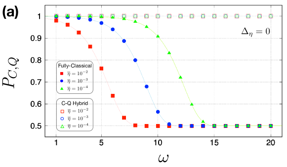
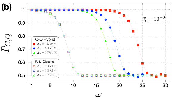
Figure 4: We plot the graphs of PC,Qsubscript𝑃𝐶𝑄P_{C,Q} versus ω𝜔\omega. The simulation is performed for randomly chosen inputs 𝐱𝐱\mathbf{x} and hsuperscripth^{\star}. In each simulation, PC,Qsubscript𝑃𝐶𝑄P_{C,Q} is evaluated by counting success and failure events over 105superscript10510^{5} queries. One single data point of PC,Qsubscript𝑃𝐶𝑄P_{C,Q} is obtained by averaging 103similar-to-or-equalsabsentsuperscript103\simeq 10^{3} trials of the simulation. (a) First, we present the simulation data of PC,Qsubscript𝑃𝐶𝑄P_{C,Q} evaluated for η¯=104¯𝜂superscript104\overline{\eta}=10^{-4}, 103superscript10310^{-3}, and 102superscript10210^{-2} with Δη=0subscriptΔ𝜂0\Delta_{\eta}=0. The results show that PCsubscript𝑃𝐶P_{C} rapidly approaches 1212\frac{1}{2} with increasing ω𝜔\omega, indicating good agreement with Eq. (6) of our main manuscript (see red, blue, and green solid lines). Meanwhile, PQsubscript𝑃𝑄P_{Q} remains unity for all the cases of η¯¯𝜂\overline{\eta}, as predicted. (b) Next, we consider the realistic situation, assuming a normal distribution 𝒩(η¯,Δη)𝒩¯𝜂subscriptΔ𝜂{\cal N}(\overline{\eta},\Delta_{\eta}). Here, we set η¯=103¯𝜂superscript103\overline{\eta}=10^{-3} with Δη=1%subscriptΔ𝜂percent1\Delta_{\eta}=1\%, 5%percent55\%, and 10%ofη¯percent10of¯𝜂10\%~{}\text{of}~{}\overline{\eta}. The data of PC,Qsubscript𝑃𝐶𝑄P_{C,Q} are shown to decay, but PQsubscript𝑃𝑄P_{Q} is much slower. In such cases, the data PQsubscript𝑃𝑄P_{Q} are well fitted by Eq. (6) of the main manuscript with ceffsubscript𝑐effc_{\text{eff}}, indicating that the data agrees well with our theoretical predictions.
      ΔηsubscriptΔ𝜂\Delta_{\eta}       η¯effsubscript¯𝜂eff\overline{\eta}_{\text{eff}} (c.f., η¯=103¯𝜂superscript103\overline{\eta}=10^{-3})       ceffsubscript𝑐effc_{\text{eff}} (c.f., c=0.5×10³𝑐0.5superscript103c=0.5\times 10^{3})
      1%ofη¯percent1of¯𝜂1\%~{}\text{of}~{}\overline{\eta}       107.63similar-to-or-equalsabsentsuperscript107.63\simeq 10^{-7.63}       0.5×107.63similar-to-or-equalsabsent0.5superscript107.63\simeq 0.5\times 10^{7.63}
      5%ofη¯percent5of¯𝜂5\%~{}\text{of}~{}\overline{\eta}       106.23similar-to-or-equalsabsentsuperscript106.23\simeq 10^{-6.23}       0.5×106.23similar-to-or-equalsabsent0.5superscript106.23\simeq 0.5\times 10^{6.23}
      10%ofη¯percent10of¯𝜂10\%~{}\text{of}~{}\overline{\eta}       105.60similar-to-or-equalsabsentsuperscript105.60\simeq 10^{-5.60}       0.5×105.60similar-to-or-equalsabsent0.5superscript105.60\simeq 0.5\times 10^{5.60}
Table 2: Detailed values of η¯effsubscript¯𝜂eff\overline{\eta}_{\text{eff}} and ceffsubscript𝑐effc_{\text{eff}} for each ΔηsubscriptΔ𝜂\Delta_{\eta}.

To corroborate and extend our theoretical predictions, we perform a numerical analysis. It starts with an input 𝐱𝐱\mathbf{x} of ω(𝐱)𝜔𝐱\omega(\mathbf{x}). We subsequently evaluate PC,Q(𝐱)subscript𝑃𝐶𝑄𝐱P_{C,Q}(\mathbf{x}) by counting the number of “h(𝐱)superscript𝐱h^{\star}(\mathbf{x})” (e.g.,, “success”) and “h(𝐱)1direct-sumsuperscript𝐱1h^{\star}(\mathbf{x})\oplus 1” (e.g.,, “failure”), such that PC,Q(𝐱)=NS/(NS+NF)subscript𝑃𝐶𝑄𝐱subscript𝑁𝑆subscript𝑁𝑆subscript𝑁𝐹P_{C,Q}(\mathbf{x})={N_{S}}/\left({N_{S}+N_{F}}\right), where NSsubscript𝑁𝑆N_{S} and NFsubscript𝑁𝐹N_{F} denote the numbers of success and failure, respectively, and NS+NF=105subscript𝑁𝑆subscript𝑁𝐹superscript105N_{S}+N_{F}=10^{5}. Here, we use the Monte-Carlo approach to mimic quantum measurement statistics. This simulation is repeated for different values of ηksubscript𝜂𝑘\eta_{k} (for kΩ𝐱𝑘subscriptΩ𝐱k\in\Omega_{\mathbf{x}}) satisfying c=(2η¯)1𝑐superscript2¯𝜂1c=(2\overline{\eta})^{-1}. This condition enables us to analyze the data statistically (i.e., by averaging over the trials) without losing generality, even though in each simulation ηksubscript𝜂𝑘\eta_{k} is changed with different hsuperscripth^{\star}. First, as an extreme but illustrative example, we consider the case of Δη=0subscriptΔ𝜂0\Delta_{\eta}=0, i.e., by assuming ηk=η¯subscript𝜂𝑘¯𝜂\eta_{k}=\overline{\eta} for all possible k=1,2,,2n𝑘12superscript2𝑛k=1,2,\ldots,2^{n}. As results, we present the graphs of PC,Qsubscript𝑃𝐶𝑄P_{C,Q} versus ω𝜔\omega as dots in Fig. 4(a) for η¯=104¯𝜂superscript104\overline{\eta}=10^{-4}, 103superscript10310^{-3}, and 102superscript10210^{-2}, where each data point of PC,Qsubscript𝑃𝐶𝑄P_{C,Q} is obtained by averaging over 103similar-to-or-equalsabsentsuperscript103\simeq 10^{3} trials. Here, it is observed that PCsubscript𝑃𝐶P_{C} decays fast to 1212\frac{1}{2}, indicating good agreement with Eq. (6) of the main manuscript. The data of PQsubscript𝑃𝑄P_{Q} are, meanwhile, shown to be unity without depending on the degree of η¯¯𝜂\overline{\eta}, as predicted. Next, we consider a realistic situation, assuming that ηksubscript𝜂𝑘\eta_{k} is drawn from a normal distribution 𝒩(η¯,Δη)𝒩¯𝜂subscriptΔ𝜂{\cal N}(\overline{\eta},\Delta_{\eta}) for all k=1,2,,2n𝑘12superscript2𝑛k=1,2,\ldots,2^{n} (and hence for kΩ𝐱𝑘subscriptΩ𝐱k\in\Omega_{\mathbf{x}}). Here, we set η¯=103¯𝜂superscript103\overline{\eta}=10^{-3} with Δη=1%subscriptΔ𝜂percent1\Delta_{\eta}=1\%, 5%percent55\%, and 10%ofη¯percent10of¯𝜂10\%~{}\text{of}~{}\overline{\eta}. The simulation results are shown in Fig. 4(b). For all cases of ΔηsubscriptΔ𝜂\Delta_{\eta}, both PCsubscript𝑃𝐶P_{C} and PQsubscript𝑃𝑄P_{Q} decay to 1212\frac{1}{2}; however, PQsubscript𝑃𝑄P_{Q} is much slower. It is also observed that the data of PQsubscript𝑃𝑄P_{Q} matched well with Eq. (6) of the main manuscript, thus allowing us to identify the effective characteristic constant ceffsubscript𝑐effc_{\text{eff}}. The identified values of ceffsubscript𝑐effc_{\text{eff}} and η¯effsubscript¯𝜂eff\overline{\eta}_{\text{eff}} are listed in Tab. 2; they manifest the predicted condition in Eq. (8) of the main manuscript.
Refer to caption
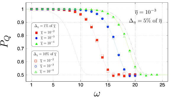
Figure 5: Graphs of PQsubscript𝑃𝑄P_{Q} with respect to ω𝜔\omega for χ¯=104¯𝜒superscript104\overline{\chi}=10^{-4}, 103superscript10310^{-3}, and 102superscript10210^{-2}. Each data point is obtained by averaging over 103superscript10310^{3} simulations. The data fitted well to Eq. (6) in the main manuscript, together with the parameter ceffsubscript𝑐effc_{\text{eff}}. The result shows that the quantum advantage becomes less pronounced as χ¯¯𝜒\overline{\chi} is increased; however, it is still highly durable. It is noteworthy that the data obtained for Δχ=1%ofχ¯subscriptΔ𝜒percent1of¯𝜒\Delta_{\chi}=1\%~{}\text{of}~{}\overline{\chi} (filled square, circle, and triangle points) and Δχ=10%ofχ¯subscriptΔ𝜒percent10of¯𝜒\Delta_{\chi}=10\%~{}\text{of}~{}\overline{\chi} (empty square, circle, and triangle points) are almost identical (up to the order of 102superscript10210^{-2}); namely, PQsubscript𝑃𝑄P_{Q} is not affected significantly by ΔχsubscriptΔ𝜒\Delta_{\chi}. The identified η¯effsubscript¯𝜂eff\overline{\eta}_{\text{eff}} and ceffsubscript𝑐effc_{\text{eff}} are listed in Tab. 2.
      χ¯¯𝜒\overline{\chi}       η¯effsubscript¯𝜂eff\overline{\eta}_{\text{eff}} (c.f., η¯=103¯𝜂superscript103\overline{\eta}=10^{-3})       ceffsubscript𝑐effc_{\text{eff}} (c.f., c=0.5×10³𝑐0.5superscript103c=0.5\times 10^{3})
      no phase-flip       106.23similar-to-or-equalsabsentsuperscript106.23\simeq 10^{-6.23}       0.5×106.23similar-to-or-equalsabsent0.5superscript106.23\simeq 0.5\times 10^{6.23}
      104superscript10410^{-4}       106.01similar-to-or-equalsabsentsuperscript106.01\simeq 10^{-6.01}       0.5×106.01similar-to-or-equalsabsent0.5superscript106.01\simeq 0.5\times 10^{6.01}
      103superscript10310^{-3}       105.34similar-to-or-equalsabsentsuperscript105.34\simeq 10^{-5.34}       0.5×105.34similar-to-or-equalsabsent0.5superscript105.34\simeq 0.5\times 10^{5.34}
      102superscript10210^{-2}       104.40similar-to-or-equalsabsentsuperscript104.40\simeq 10^{-4.40}       0.5×104.40similar-to-or-equalsabsent0.5superscript104.40\simeq 0.5\times 10^{4.40}
Table 3: Detailed values of η¯effsubscript¯𝜂eff\overline{\eta}_{\text{eff}} and ceffsubscript𝑐effc_{\text{eff}} for each χ¯¯𝜒\overline{\chi}.

For a more realistic condition, we consider another type of error, i.e., phase-flip in the assistant qubit that would be crucial for maintaining a higher success rate of the query. In particular, we assume that the phase-flip errors primarily occur when the qubit travels between a^ksubscript^𝑎𝑘\hat{a}_{k} and a^k+1subscript^𝑎𝑘1\hat{a}_{k+1} with a certain probability χk12subscript𝜒𝑘12\chi_{k}\leq\frac{1}{2}. First, when Δη=0subscriptΔ𝜂0\Delta_{\eta}=0 (or equivalently, ηk=η¯subscript𝜂𝑘¯𝜂\eta_{k}=\overline{\eta}) for all k𝑘k, the phase-flip errors do not affect the query process and PQsubscript𝑃𝑄P_{Q} becomes unity. In the realistic case, namely of Δη0subscriptΔ𝜂0\Delta_{\eta}\neq 0, however, it is predicted that the amplitudes of the bit-flip errors would interfere disorderly owing to the phase-flip, and eventually the quantum advantage becomes smaller, as described in our main manuscript. Thus, we perform the simulations and present the data of PQsubscript𝑃𝑄P_{Q} in Fig. 5. Here, χksubscript𝜒𝑘\chi_{k} is assumed to be drawn from 𝒩(χ¯,Δχ)𝒩¯𝜒subscriptΔ𝜒{\cal N}(\overline{\chi},\Delta_{\chi}) for all k=1,2,,2n𝑘12superscript2𝑛k=1,2,\ldots,2^{n}. The simulation data are generated for χ¯=104¯𝜒superscript104\overline{\chi}=10^{-4}, 103superscript10310^{-3} and 102superscript10210^{-2}. Here, we set η¯=103¯𝜂superscript103\overline{\eta}=10^{-3} with Δη=5%ofη¯subscriptΔ𝜂percent5of¯𝜂\Delta_{\eta}=5\%~{}\text{of}~{}\overline{\eta}. The data are well fitted by Eq. (6) of our main manuscript, and ceffsubscript𝑐effc_{\text{eff}} are well estimated from the data (see Tab. 3). As expected, the quantum advantage becomes less pronounced as χ¯¯𝜒\overline{\chi} is increased; however, it can still exhibit a higher success rate of the query. It is noteworthy that the data obtained for both Δχ=1%and10%ofχ¯subscriptΔ𝜒percent1andpercent10of¯𝜒\Delta_{\chi}=1\%~{}\text{and}~{}10\%~{}\text{of}~{}\overline{\chi} are almost identical (up to the second digit of a decimal).

Appendix C: Reduction in learning sample complexity in the framework of probably-approximately-correct (PAC) learning

In a probably-approximately-correct (PAC) learning model, a learner (or equivalently, a learning algorithm) samples a finite set of training data {(𝐱i,h(𝐱i))}subscript𝐱𝑖superscriptsubscript𝐱𝑖\{(\mathbf{x}_{i},h^{\star}(\mathbf{x}_{i}))\} (i=1,2,,M𝑖12𝑀i=1,2,\ldots,M) by accessing an oracle, aiming at obtaining the best hypothesis hh close to hsuperscripth^{\star} for a given set, e.g., H𝐻{H}, of the hypothesis hh. Here, 𝐱isubscript𝐱𝑖\mathbf{x}_{i} is typically assumed to be drawn uniformly. Subsequently, a learning algorithm is a (ϵitalic-ϵ\epsilon, δ𝛿\delta)-PAC learner (under uniform distribution), if the algorithm obtains an ϵitalic-ϵ\epsilon-approximated correct hh with probability 1δ1𝛿1-\delta; more specifically, satisfying

P[E(h,h)ϵ]1δ,𝑃delimited-[]𝐸superscriptitalic-ϵ1𝛿\displaystyle P[E(h,h^{\star})\leq\epsilon]\geq 1-\delta, (26)

where E(h,h)𝐸superscriptE(h,h^{\star}) denotes the error. Here, if hh identified by the algorithm agrees with

M1ϵln|H|δ𝑀1italic-ϵ𝐻𝛿\displaystyle M\geq\frac{1}{\epsilon}\ln{\frac{{\left|H\right|}}{\delta}} (27)

of samples constructed from the oracle, then Eq. (26) holds. Here, |H|22n𝐻superscript2superscript2𝑛\left|H\right|\leq 2^{2^{n}} denotes the cardinality of H𝐻{H}. Eq. (27) is known as the bound of the sample complexity Valiant84 ; Langley95 , i.e., it yields the minimum number of training samples to successfully learn hH𝐻h\in{H} satisfying Eq. (26). Such a sample complexity bound derived from the previous studies can directly be carried over to our scenario; in our classical–quantum hybrid query scheme, the same sample complexity bound exists, because 𝐱isubscript𝐱𝑖\mathbf{x}_{i} and h(𝐱i)superscriptsubscript𝐱𝑖h^{\star}(\mathbf{x}_{i}) identified by the measurement on |ψout(𝐱i)ketsubscript𝜓outsubscript𝐱𝑖\left|\psi_{\text{out}}(\mathbf{x}_{i})\right> are classical.

However, in the case where the oracle is not perfect, the bound of sample complexity in Eq. (27) is modified as follows: First, we draw a sequence of the training data {(𝐱1,m1),(𝐱2,m2),,(𝐱M,mM)}subscript𝐱1subscript𝑚1subscript𝐱2subscript𝑚2subscript𝐱𝑀subscript𝑚𝑀\{(\mathbf{x}_{1},m_{1}),(\mathbf{x}_{2},m_{2}),\ldots,(\mathbf{x}_{M},m_{M})\} sampled from our classical–quantum hybrid oracle, where mi{h(𝐱i),h(𝐱i)1}subscript𝑚𝑖superscriptsubscript𝐱𝑖direct-sumsuperscriptsubscript𝐱𝑖1m_{i}\in\{h^{\star}(\mathbf{x}_{i}),h^{\star}(\mathbf{x}_{i})\oplus 1\} denotes the outcome of the measurement performed on |ψout(𝐱i)ketsubscript𝜓outsubscript𝐱𝑖\left|\psi_{\text{out}}(\mathbf{x}_{i})\right>. Subsequently, if the sampling is performed with

M2AQln(2|H|δ)1ϵ2,\displaystyle M\geq 2A_{Q}\ln{\left(\frac{2\left|H\right|}{\delta}\right)^{\frac{1}{\epsilon^{2}}}}, (28)

we can verify that Eq. (26) holds for the algorithm that obtains hh maximizing P¯Qsubscript¯𝑃𝑄\overline{P}_{Q}. In fact, it has been proven that the additional factor AQsubscript𝐴𝑄A_{Q} is given as Angluin94

AQ=1(2P¯Q(n)1)2.subscript𝐴𝑄1superscript2subscript¯𝑃𝑄𝑛12\displaystyle A_{Q}=\frac{1}{\left(2\overline{P}_{Q}(n)-1\right)^{2}}. (29)

It is noteworthy that in the purely classical case, the corresponding factor, e.g., ACsubscript𝐴𝐶A_{C}, is given with P¯Csubscript¯𝑃𝐶\overline{P}_{C} instead of P¯Qsubscript¯𝑃𝑄\overline{P}_{Q}. Thus, we can derive the reduction in the sample complexity with the condition AQACsubscript𝐴𝑄subscript𝐴𝐶A_{Q}\leq A_{C} from P¯QP¯Csubscript¯𝑃𝑄subscript¯𝑃𝐶\overline{P}_{Q}\geq\overline{P}_{C}. To view this explicitly, we rewrite AQsubscript𝐴𝑄A_{Q} in Eq. (29) to a more useful form:

AQ=[12nω=0n(nω)e2ωγc]2=[j=0(1)jj!(1γc)j(2j+12)n]2subscript𝐴𝑄superscriptdelimited-[]1superscript2𝑛superscriptsubscript𝜔0𝑛binomial𝑛𝜔superscript𝑒superscript2𝜔𝛾𝑐2superscriptdelimited-[]superscriptsubscript𝑗0superscript1𝑗𝑗superscript1𝛾𝑐𝑗superscriptsuperscript2𝑗12𝑛2\displaystyle A_{Q}=\left[\frac{1}{2^{n}}\sum_{\omega=0}^{n}{{n}\choose{\omega}}e^{-\frac{2^{\omega}}{\gamma c}}\right]^{-2}=\left[\sum_{j=0}^{\infty}\frac{(-1)^{j}}{j!}\left(\frac{1}{\gamma c}\right)^{j}\left(\frac{2^{j}+1}{2}\right)^{n}\right]^{-2} (30)

This implies that a small increment in the sample complexity bound when n𝑛n is small increases abruptly from near n2log2γcsimilar-to-or-equals𝑛2subscript2𝛾𝑐n\simeq 2\log_{2}{\gamma c}. As ACsubscript𝐴𝐶A_{C} is characterized by c𝑐c without γ𝛾\gamma, we can interpret γ𝛾\gamma as a quantum learning advantage in the PAC learning framework; i.e., for any large n𝑛n, we can define a (ϵitalic-ϵ\epsilon, δ𝛿\delta)-PAC learner with our hybrid oracle, unlike with a fully classical one. It is noteworthy that if n𝑛n is excessively large, i.e., when n2log2γcmuch-greater-than𝑛2subscript2𝛾𝑐n\gg 2\log_{2}{\gamma c}, it is impractical to define a legitimate PAC learner even with our hybrid oracle. This result is consistent with the recent theoretical study in Ref. Cross15 ; however, in our case, such a quantum learning advantage is achieved with classical data.

To corroborate and extend our analysis, numerical simulations are performed: For a given n𝑛n, we prepare a set of inputs {𝐱1,𝐱2,,𝐱M}subscript𝐱1subscript𝐱2subscript𝐱𝑀\{\mathbf{x}_{1},\mathbf{x}_{2},\ldots,\mathbf{x}_{M}\} that is sampled randomly. For the given ω(𝐱i)𝜔subscript𝐱𝑖\omega(\mathbf{x}_{i}) (i=1,2,,M𝑖12𝑀i=1,2,\ldots,M), we evaluate PC,Q(ω)subscript𝑃𝐶𝑄𝜔P_{C,Q}(\omega) by counting 105superscript10510^{5} queries and identify their average value, i.e., 1105i=1105PC,Q(ω(𝐱i))1superscript105superscriptsubscript𝑖1superscript105subscript𝑃𝐶𝑄𝜔subscript𝐱𝑖\frac{1}{10^{5}}\sum_{i=1}^{10^{5}}P_{C,Q}(\omega(\mathbf{x}_{i})). This process is repeated 103similar-to-or-equalsabsentsuperscript103\simeq 10^{3} times for different input sets to analyze P¯C,Q(n)subscript¯𝑃𝐶𝑄𝑛\overline{P}_{C,Q}(n) statistically. The data are generated from n=8𝑛8n=8 to n=35𝑛35n=35, assuming that ηksubscript𝜂𝑘\eta_{k} and χksubscript𝜒𝑘\chi_{k} (kfor-all𝑘\forall k) are drawn from 𝒩(η¯,Δη)𝒩¯𝜂subscriptΔ𝜂{\cal N}(\overline{\eta},\Delta_{\eta}) and 𝒩(χ¯,Δχ)𝒩¯𝜒subscriptΔ𝜒{\cal N}(\overline{\chi},\Delta_{\chi}), respectively. Here, we consider η¯=103¯𝜂superscript103\overline{\eta}=10^{-3} with Δη=0.05η¯subscriptΔ𝜂0.05¯𝜂\Delta_{\eta}=0.05\overline{\eta} and χ¯=102¯𝜒superscript102\overline{\chi}=10^{-2} with Δχ=0.1χ¯subscriptΔ𝜒0.1¯𝜒\Delta_{\chi}=0.1\overline{\chi}. In each simulation, M𝑀M is fixed to 100100100. The obtained data agree well with our theoretical predictions (see Figs. 2(a) and 2(b) in the main manuscript).

References

  • (1) Shor, P. W.: Polynomial-time algorithms for prime factorization and discrete logarithms on a quantum computer. SIAM Review 41(2), 302-332 (1999).
  • (2) Grover, L.K.: Quantum mechanics helps in searching for a needle in a haystack. Phys. Rev. Lett. 79, 325 (1997).
  • (3) Harrow, A. W., Hassidim, A. and Lloyd, S.: Quantum algorithm for linear systems of equations. Phys. Rev. Lett. 103, 150502 (2009).
  • (4) Giovannetti, V., Lloyd, S. and Maccone, L.: Quantum random access memory. Phys. Rev. Lett. 100, 160501 (2008).
  • (5) Giovannetti, V., Lloyd, S. and Maccone, L.: Architectures for a quantum random access memory. Phys. Rev. A 78, 052310 (2008).
  • (6) Aaronson, S.: Read the find print. Nature Physics 11, 291 (2015).
  • (7) Arunachalam, S., Gheorghiu, V., Jochym-O’Connor, T., Mosca, M. and Srinivasan, P. V.: On the robustness of bucket brigade quantum RAM. New Journal of Physics 17, 123010 (2015)
  • (8) Ciliberto, C., Herbster, M., Ialongo, A. D., Pontil, M., Rocchetto, A., Severini, S. and Wossnig, L.: Quantum machine learning: a classical perspective. Proc. R. Soc. A 474, 20170551 (2018).
  • (9) Preskill, J.: Quantum Computing in the NISQ era and beyond. Quantum 2, 79 (2018).
  • (10) Arute, F. et al.: Quantum supremacy using a programmable superconducting processor. Nature 574, 505 (2019).
  • (11) Peruzzo, A., McClean, J. R., Shadbolt, P., Yung, M. H., Zhou, X. Q., Love, P. J., Aspuru-Guzik, A. and O’brien, J. L.: A variational eigenvalue solver on a photonic quantum processor. Nature communications 5, 4213 (2014).
  • (12) McClean, J. R., Romerom J., Babbush, R. and Aspuru-Guzik, A.: The theory of variational hybrid quantum-classical algorithms. New Journal of Physics 18, 023023 (2016).
  • (13) Khoshaman, A., Vinci, W., Denis, B., Andriyash, E. and Amin, M. H.: Quantum variational autoencoder. Quantum Science and Technology 4, 014001 (2018).
  • (14) Zhu, D. et al.: Training of quantum circuits on a hybrid quantum computer. Science Advances 5(10) (2019).
  • (15) Havlíček, V., Córcoles, A. D., Temme, K., Harrow, A. W., Kandala, A., Chow, J. M. and Gambetta, J. M.: Supervised learning with quantum-enhanced feature spaces. Nature 567, 209 (2019).
  • (16) Yoo, S., Bang, J., Lee, C. and Lee, J.: A quantum speedup in machine learning: Finding a N-bit Boolean function for a classification. New Journal of Physics 16, 103014 (2014).
  • (17) Lee, J. S., Bang, J., Hong, S., Lee, C., Seol, K. H., Lee, J. and Lee, K. G.: Experimental demonstration of quantum learning speedup with classical input data. Phys. Rev. A 99, 012313 (2019).
  • (18) Bang, J., Dutta, A., Lee, S. W. and Kim, J.: Optimal usage of quantum random access memory in quantum machine learning. Phys. Rev. A 99, 012326 (2019).
  • (19) Dunjko, V., Ge, Y. and Cirac, J. I.: Computational speedups using small quantum devices. Phys. Rev. Lett. 121, 250501 (2018).
  • (20) Harrow, A. W.: Small quantum computers and large classical data sets. arXiv preprint arXiv:2004.00026 (2020).
  • (21) Buhrman, H., Newman, I., Rohrig, H. and de Wolf, R.: Robust polynomials and quantum algorithms. Theory of Computing Systems 40, 379 (2007).
  • (22) Cross, A. W., Smith, G. and Smolin, J. A.: Quantum learning robust against noise. Phys. Rev. A 92, 012327 (2015).
  • (23) Valiant, L. G.: A theory of the learnable. Communications of the ACM 27, 1134 (1984)
  • (24) Langley, P.,: Elements of machine learning, (Morgan Kaufmann) (1995)
  • (25) Ambainis, A., Iwama, K., Kawachi, A., Masuda, H., Putra, R. H. and Yamashita, S.: Quantum identification of Boolean oracles. Annual Symposium on Theoretical Aspects of Computer Science, Springer pp. 105–116 (2004).
  • (26) Childs, A. M., Kothari, R., Ozols, M. and Roetteler, M.: Easy and hard functions for the Boolean hidden shift problem. 8th Conference on the Theory of Quantum Computation, Communication and Cryptography (TQC 2013) (Dagstuhl, Germany: Schloss Dagstuhl–Leibniz-Zentrum fuer Informatik) vol. 22 of Leibniz International Proceedings in Informatics (LIPIcs) pp. 50–79 (2013).
  • (27) Arunachalam, S. and de Wolf, R.: Guest column: A survey of quantum learning theory. ACM SIGACT News 48, 41 (2017).
  • (28) Gupta, P., Agrawal, A. and Jha, N. K.: An algorithm for synthesis of reversible logic circuits. IEEE Transactions on Computer-Aided Design of Integrated Circuits and Systems 25, 2317 (2006).
  • (29) Angluin, D. and Laird, P.: Queries and concept learning. Machine Learning 2(4), 319 (1988).
  • (30) Angluin, D. and Slonim, D. K.: Randomly fallible teachers: Learning monotone DNF with an incomplete membership oracle. Machine Learning 14(1), 7 (1994)
  • (31) Bshouty, N. H. and Jackson, J. C.: Learning DNF over the uniform distribution using a quantum example oracle. SIAM Journal on Computing 28, 1136 (1998).
  • (32) Toffoli, T.: Reversible computing. International Colloquium on Automata, Languages, and Programming. Springer pp. 632–644 (1980).
  • (33) Younes, A. and Miller, J. F.: Representation of Boolean quantum circuits as Reed–Muller expansions. International journal of electronics 91, 431 (2004)
  • (34) Van Dam, W.: Quantum oracle interrogation: Getting all information for almost half the price. Proceedings 39th Annual Symposium on Foundations of Computer Science (Cat. No. 98CB36280) IEEE pp. 362–367 (1998)
  • (35) Debnath, S., Linke, N. M., Figgatt, C., Landsman, K. A., Wright, K. and Monroe, C.: Demonstration of a small programmable quantum computer with atomic qubits. Nature 536, 63 (2016).
  • (36) Eleuch, H., Hilke, M. and MacKenzie, R.: Probing Anderson localization using the dynamics of a qubit. Phys. Rev. A 95, 062114 (2017).
  • (37) Hanneke, S.: The optimal sample complexity of PAC learning. The Journal of Machine Learning Research 17, 1319 (2016).