Gaussian Lattice Boltzmann method and its applications to rarefied flows

Abstract

A novel discretization approach for the Bhatnager-Gross-Krook (BGK) kinetic equation is proposed. A hierarchy of LB models starting from $D1Q3$ model with increasing number of velocities converging to BGK model is derived. The method inherits properties of the Lattice Boltzmann (LB) method like linear streaming step, conservation of moments. Similar to the finite-difference methods for the BGK model the presented approach describes high-order moments of the distribution function with controllable error. The Sod shock tube problem, the Poiseuille flow between parallel plates and the plane Couette flow are considered for wide range of Knudsen numbers. Good stability and significant increase in precision over the conventional LB models are observed.

Keywords: Lattice Boltzmann method, rarefied flows, non-equilibrium flows

1 Introduction

Nowadays the Lattice Boltzmann (LB) approach [1, 2, 3] is supposed to be an useful tool in modeling of non-equilibrium rarefied flows [4, 5, 6, 7, 8, 9, 10, 11, 12, 13, 14, 15, 16, 17]. Nevertheless, when the flow is rarefied and the role of high-order moments of the velocity distribution function increases the precision of conventional LB models go down.

In the conventional LB method the discretization is performed in a such way that the LB distribution function is equivalent to the solution for the BGK equation projected on a finite basis in a velocity space spanned by the Hermite polynomials (the Grad expansion). This equivalence is achieved via the Gauss-Hermite quadratures [18, 19, 20, 21]. Since the first moments of the LB local equilibrium are reproduced in the same form as for the local Maxwell state then LB method is conservative by the construction. The application of an additional regularization procedure [22, 23, 24] guarantees that the solutions of LB will be confined in this finite velocity space and results in increased stability and precision of the LB models [5, 7, 25, 26, 15].

Instead of the exact reproduction of the first moments for the local Maxwell state, the finite-difference methods for the BGK model are aimed to recover the distribution function in overall with decreasing error when the discrete velocity set is growing [27]. Potentially all the moments of the distribution function are recovered but with some error. The cost to pay is the usage of relatively large discrete velocity sets, moreover conservation of the first moments requires some additional efforts and the streaming step does not have concise form like in the LB method.

The present research is aimed to develop a new LB based discrete velocity (DV) method which is able to cope with the kinetic high-order moments in the rarefied flow but without drastic increase in number of discrete velocities. The starting point of the presented construction is a well-known one-dimensional three-velocity $D1Q3$ LB model [28]. At the next step, a summation procedure for the LB model is introduced: an addition of $D1Q3$ model to $D1Q3$ model yields $D1Q5$ model. The repetition of the summation $k$ times leads to models with $(3+2k)$ velocities. All the models in the hierarchy have the same order of the isotropy equals to the order of the isotropy of the root model ($D1Q3$), moreover the models are calibrated at the same flow velocity and temperature. The models in the hierarchy have monotonically increasing precision in a following sense. The magnitudes of the errors in all highest moments (in the comparison with the local Maxwell state) are uniformly decreasing when $k$ is growing. Using the Central Limit Theorem (CLT) one can show that the hierarchy of LB models converges to the BGK model. The presented method covers advantageous properties of the both DV and LB methods. The Gaussian shape of the local equilibrium state is better reproduced in each subsequent summation step which results in better reproduction of the half-moments and the kinetic boundary conditions.

The numerical experiments presented in Section 5 support the theoretical predictions. The models show good stability in the Sod shock tube problem. For the the plane Couette flow and Poiseuille flow between parallel walls the convergence to the benchmark solutions is observed.

2 The Construction of the Hierarchy of Lattice Boltzmann models and Central Limit Theorem

The simplest LB one-dimensional discretization of the BGK equation which is able to reproduce the Navier-Stokes equations at the limit of low Mach numbers $Ma$ (with $O(Ma^{3})$ error) is D1Q3 model [28]

$$f_{i}(t+\Delta t,x+c_{i}\Delta t)-f_{i}(t,x)=\frac{\Delta t}{\tau+\frac{\Delta t}{2}}\left(f^{eq}_{i}-f_{i}\right)(t,x),$$

where $\tau$ is the relaxation time, $f_{i},i=-1,0,1$ are the lattice distribution functions corresponding to the lattice velocities $c_{i}:-c,0,+c$, here $c\Delta t$ is the distance between the lattice nodes, $\Delta t$ is the lattice time step. The form of a collision frequency $\frac{1}{\tau+\frac{\Delta t}{2}}$ guarantees second-order accuracy in physical space [28]. The equilibrium states $f^{eq}_{\pm 1},f^{eq}_{0}$ are defined as

$$f^{eq}_{\pm 1}(t,x)=\frac{\rho(t,x)}{6}\left(1\pm 3\frac{u(t,x)}{c}+3\frac{u(t,x)^{2}}{c^{2}}\right),$$

$$f^{eq}_{0}(t,x)=\frac{4\rho(t,x)}{6}\left(1-3\frac{u(t,x)^{2}}{2c^{2}}\right),$$

where the macroscopic parameters $\rho,u$ are defined from the expressions

$$\rho(t,x)=f_{-1}(t,x)+f_{0}(t,x)+f_{+1}(t,x),$$

$$\rho(t,x)u(t,x)=-f_{-1}(t,x)c+f_{+1}(t,x)c,$$

moreover the full energy is calculated as follows

$$\rho(t,x)(u(t,x)^{2}+c_{s}^{2})=(f_{-1}(t,x)+f_{+1}(t,x))c^{2},$$

where the sound velocity is fixed: $c_{s}=\sqrt{\frac{1}{3}}c$, i.e. the model describes only isothermal flows. This model serves as a root of the presented below hierarchy.

Now lets associate with the local equilibrium distribution function for $D1Q3$ model a random variable $X(N)$, here $N=1$ (the first step in the hierarchy). Assume that this random variable has three outcomes $-c(1),0,+c(1)$, where $c(1)$ is some lattice velocity. Assume that $X(1)$ has the distribution function same as the local equilibrium distribution for $D1Q3$ model. At the present moment this procedure is formal and does not give any additional information. The underlying reason for the introduction of the random variable $X(1)$ will be clear at the next step.

Next, consider two independent identically distributed (i.i.d.) random variables $X_{1}(2),X_{2}(2)$ (here $N=2$ , the second step) where each of the variables has again three outcomes $-c(2),0,+c(2)$ in a such way that their sum has the same expected value (the bulk velocity $u$) and the same variance (the temperature $c_{s}^{2}$) as for $N=1$ case.

Now, generalizing the previous step consider a sum of $N$ i.i.d. random variables (each has three outcomes $-c(N),0,+c(N)$) such that their sum has an expected value $u$ and variance $c_{s}^{2}$. The variable $\sum_{j}^{N}X_{j}(N)$ has $2N+1$ possible outcomes $-Nc,(-N+1)c\ldots Nc,\,c\equiv c(N)$. Since this sum is composed of the independent identical random variables then the corresponding distribution function can be calculated in an exact closed form. As a result, a triangular array of the random variables can be constructed

$$X(1),$$

$$X_{1}(2),X_{2}(2),$$

$$X_{1}(3),X_{2}(3),X_{3}(3),$$

$$\ldots\ldots\ldots\ldots$$

$$X_{1}(2),X_{2}(2),\ldots\ldots X_{N}(N).$$

The Central Limit Theorem (CLT) for triangular arrays in the form of Lyapunov or Lindeberg-Feller [29] guarantees that the sequence of the distribution functions in the hierarchy converges to the Gaussian distribution (the Maxwell state with the bulk velocity $u$ and the temperature $c_{s}^{2}$).

It will be convenient to define as $Prob\left(\sum_{j=1}^{N}X_{j}=nc\right)$ a probability for a sum of $N$ random variables $X_{j}(N),j=1\ldots N$ to have a value $nc(N),n=-N\ldots N$.

The evaluation of $Prob\left(\sum_{j=1}^{N}X_{j}=nc\right)$ can be reduced to the following problem. Assume that a dice is rolled $N$ times, each dice roll has three outcomes $0,\pm 1$ with the probabilities $p_{0},p_{\pm}$. One needs to find the probability that a sum of rolls take the value $n,|n|\leq N$. Assume that $n\geq 0$ (the case of negative $n$ can be considered in a similar way) and the value $-1$ is obtained $m$ times. Then the value $1$ is rolled $n+m$ times, and the value $0$ is obtained $N-(n+m)-m\geq 0$ times. The latter inequality means that $m$ is lesser than $(N-m)/2$. Since $m$ can take only integer values then $m$ lies in the interval from $0$ to $\lfloor\frac{N-n}{2}\rfloor$. The number of ways to get $-1$ result $m$ times and $1,0$ results $n+m,N-n-2m$ times respectively is $N!/(n+m)!m!(N-n-2m)!$. Then the required probability is $\sum_{m=0}^{\lfloor\frac{N-n}{2}\rfloor}\frac{N!}{(n+m)!m!(N-n-2m)!}p_{+}^{n+m}p_{-}^{m}p_{0}^{N-n-2m}$ .

Finally, at $N$-s step ($N-1$ summations) the following $2N+1$ discrete velocity model is introduced for $-Nc,(-N+1)c\ldots Nc,\,c\equiv c(N)$ lattice

$$f_{n}(t+\Delta t,x+nc\Delta t)-f_{n}(t,x)=\frac{\Delta t}{\tau+\frac{\Delta t}{2}}\left(f^{eq}_{n;N}-f_{n}\right)(t,x),$$ (1)

where $n=-N\ldots N$ and

$$f^{eq}_{n;N}(t,x)=\rho Prob\left(\sum_{j=1}^{N}X_{j}=nc\right),$$ (2)

$$Prob\left(\sum_{j=1}^{N}X_{j}=nc\right)=$$

$$=\sum_{m=0}^{\lfloor\frac{N-n}{2}\rfloor}\frac{N!}{(n+m)!m!(N-n-2m)!}P_{N,+}^{n+m}P_{N,-}^{m}P_{N,0}^{N-n-2m}$$ (3)

for $n\geq 0$ , where $\lfloor\cdot\rfloor$ is the rounding to lowest integer and

$$P_{N,\pm}=\frac{1}{2c^{2}N}\left(c_{s}^{2}\pm cu+\frac{u^{2}}{N}\right),$$ (4)

$$P_{N,0}=1-P_{N,+}-P_{N,-}$$ (5)

and

$$c_{s}^{2}=\frac{Nc^{2}}{3},$$ (6)

where for the sake of brevity the shortened notation for the lattice velocity $c$ is used instead of $c(N)$. To keep the temperature constant $c_{s}^{2}=\theta_{0}$ at the all levels of the hierarchy it should be required

$$c\equiv c(N)=\sqrt{3\theta_{0}/N},$$ (7)

thus the lattice step is decreasing when $N$ grows. Similar expressions can be obtained for $n<0$ by taking $|n|$ instead of $n$ and changing $P_{N,\pm}$ by $P_{N,\mp}$. For the sake of clarity an example for $N=2$ case is addressed in Appendix A. One can convince that the shape of the equilibrium states $f^{eq}_{n;N}$ readily converges to Gaussian after a few summation steps.

The model (1)-(6) is the main result of the paper. It can considered as a new LB type discretization for the BGK kinetic equation (for isothermal flows).

3 Analytical properties

The equilibrium states in the hierarchy contain the functions $P_{N,\pm},P_{N,0}$. This states are non-negative if $P_{N,\pm},P_{N,0}$ are non-negative. This requirement leads to the following inequality $|u|\leq\sqrt{\frac{2}{3}}Nc$ or $|u|\leq\sqrt{2N\theta_{0}}$. Therefore, the domain of non-negativity is growing when $N$ increases. Potentially this property can result in better stability for the models with $N>1$ in comparison with the conventional $D1Q3$ model.

The most interesting question is the reproduction of the highest moments of the local Maxwell state by the presented method. By a straightforward computation one can convince that the difference between the third moment for the local Maxwell distribution and the third moment for $N$-s model in the hierarchy is

$$\frac{u^{3}}{N^{2}}.$$

The order of isotropy is constant in the hierarchy but the overall magnitude of the error is decreasing as $N^{-2}$. This is very similar to the finite-difference methods for BGK model, for which the errors appear in all moments but they are suppressed at some rate when the number of discrete velocities is growing.

The fourth moment behaves in a similar way. For the difference between the local Maxwell fourth moment and the fourth moment for the local equilibrium states in the hierarchy one has the expression

$$\frac{\theta_{0}u^{2}}{N^{2}}-\left(\frac{4}{N^{2}}+\frac{3}{N^{3}}\right)u^{4},$$

and again similarly to the $D1Q3$ model all the models in the hierarchy have $O(u^{2})$ leading error term. The amplitude of the errors decrease as $N^{-2}$.

The straightforward computation of the moment generating function (MGF) defined by $M(s)$ is complicated. One has

$$M(s)\equiv<e^{ns}>=\sum_{n=-N}^{N}e^{ns}Prob\left(\sum_{j=1}^{N}X_{j}=nc\right).$$

The convolution of the sums seems to be problematic. Nevertheless, the result can be obtained if one takes in account the fact that the local equilibrium is related to a sum $Y=\sum^{N}_{j}X_{j}(N)$ of independent random variables $X_{j}(N)$. Then the moment generating function for $Y$ is a product of the moment generating functions for $X_{j}(N)$, they are defined below as $M_{X}(s)$. As a result

$$M(s)=M_{X}(s)^{N}=(P_{N,-}e^{-cs}+P_{N,0}+P_{N,+}e^{cs})^{N},$$ (8)

then any moment $m_{k}$ of order $k$ can be calculated from Eq. (8) using the formula

$$m_{k}=\frac{d^{k}M(s)}{ds^{k}}|_{s=0}.$$

Now taking logarithm from the MGF function (8) and using the expressions (4) one obtains the following expression

$$\log(M(s))=\frac{\theta s^{2}}{2}+us+$$

$$+\left\{(9/6!-1/16)s^{6}+\ldots+(-u^{3}/2)s^{3}\right\}\frac{1}{N^{2}}+O\left(\frac{1}{N^{3}}\right),$$

where $\frac{\theta s^{2}}{2}+us$ is the logarithm of MGF for the Gaussian distribution and $\theta$ is some constant temperature. Therefore, the difference between the logarithms of MGF for the LB local equilibrium state in Eqs. (1)-(6) and the local Maxwell state is of $O(1/N^{2})$ order. Then one concludes that the moments for the presented LB models converge to the local Maxwell ones with the error decreasing as $O(1/N^{2})$.

4 Models in several dimensions and ballistic streamers removal

The models in several dimensions can be constructed as a tensor product of 1D models. It will be convenient to denote the models based on the presented summation procedure as $G$-$DaQb$ (Gaussian LB model in $a$ dimensions with $b$ velocities). Since all the models in the discussed above hierarchy have the same order of isotropy ($D1Q3$, $G$-$D1Q5$, $G$-$D1Q7$ and so on) then one can construct 2D and 3D models in the form $G$-$D1Qn\times G$-$D1Qm$ and $G$-$D1Qn\times G$-$D1Qm\times G$-$D1Qk$ with $n*m$, $n*m*k$ velocities respectively, the order of isotropy for the multidimensional models will be the same as in 1D case. The local equilibrium takes the product form of the equilibrium states for 1D models. This product form approach is based on the ideas from [30].

For instance, the simplest multidimensional model (2D case) is $15$ velocity model $G$-$D2Q15$ composed by the $G$-$D1Q5$ (the formal sum of $D1Q3$ and $D1Q3$) and $D1Q3$ model.

This models have velocities parallel to the axis - a streaming directions which do not collide with a wall if the wall is placed parallel to the axis (ballistic streamers effect) [4]. The removal of zero lattice velocity mitigates the problem and significantly increases the calculation precision for several problems [4, 16].

Having $(2N+1)$ velocity model for $[-Nc\ldots 0\ldots Nc]$ lattice the transformation to $(2N+2)$ velocity model (zero velocity is removed) for $[-(N+0.5)c,-(N-0.5)c,\ldots(N-0.5)c,(N+0.5)c]$ lattice is proposed. Here the lattice step $c$ is not fixed by the relation (7) since another relation between the temperature and lattice velocity will be obtained. This model reads as

$$f_{n+\frac{1}{2}}\left(t+\Delta t,x+\left(n+\frac{1}{2}\right)c\Delta t\right)-f_{n+\frac{1}{2}}(t,x)=$$

$$=\frac{\Delta t}{\tau+\frac{\Delta t}{2}}\left(f^{eq}_{n+\frac{1}{2};N}-f_{n+\frac{1}{2}}\right)(t,x),\quad n=0\ldots N,$$

$$f_{n-\frac{1}{2}}\left(t+\Delta t,x+\left(n-\frac{1}{2}\right)c\Delta t\right)-f_{n-\frac{1}{2}}(t,x)=$$

$$=\frac{\Delta t}{\tau+\frac{\Delta t}{2}}\left(f^{eq}_{n-\frac{1}{2};N}-f_{n-\frac{1}{2}}\right)(t,x),\quad n=-N,$$

where $f_{n+\frac{1}{2}},f_{n+\frac{1}{2};N}^{eq}$ are the distribution functions and local equilibrium states for the lattice velocities $(n+\frac{1}{2})c,\,n=0\ldots N$; $f_{n-\frac{1}{2}},f_{n-\frac{1}{2};N}^{eq}$ are the distribution functions and local equilibrium states for the lattice velocities $(n-\frac{1}{2})c,\,n=-N\ldots 0$.

Here the values of $f_{\pm n\pm\frac{1}{2};N}^{eq}$ are taken as the average value of the local distribution states from $2N+1$ hierarchy for the neighbouring to $(\pm n\pm\frac{1}{2})c$ lattice velocities $\pm nc$ and $\pm(n+1)c$

$$f_{n+\frac{1}{2};N}^{eq}\left(nc+\frac{1}{2}c\right)=\frac{1}{2}\left\{f_{n+1;N}^{eq}(nc+c)+f_{n;N}^{eq}(nc)\right\},$$ (9)

valid for $0\leq n<N$ and

$$f_{N+\frac{1}{2};N}^{eq}\left(Nc+\frac{1}{2}c\right)=\frac{1}{2}f_{N;N}^{eq}(Nc),$$ (10)

also

$$f_{n-\frac{1}{2};N}^{eq}\left(nc-\frac{1}{2}c\right)=\frac{1}{2}\left\{f_{n-1;N}^{eq}(nc-c)+f_{n;N}^{eq}(nc)\right\}$$ (11)

valid for $-N<n\leq 0$ and

$$f_{-N-\frac{1}{2};N}^{eq}\left(-Nc-\frac{1}{2}c\right)=\frac{1}{2}f_{-N;N}^{eq}(-Nc),$$ (12)

where $f_{n,N}^{eq}$ are the local equilibrium states from $2N+1$ velocities hierarchy (4). One can convince that

$$\sum_{n=-N}^{0}f_{n-\frac{1}{2};N}^{eq}+\sum_{n=0}^{N}f_{n+\frac{1}{2};N}^{eq}=\sum_{n=-N}^{N}f_{n;N}^{eq}=\rho$$

and

$$\sum_{n=-N}^{0}f_{n-\frac{1}{2};N}^{eq}\left[nc-\frac{1}{2}c\right]+\sum_{n=0}^{N}f_{n+\frac{1}{2};N}^{eq}\left[nc+\frac{1}{2}c\right]=$$

$$=\sum_{n=-N}^{N}f^{eq}_{n;N}nc=\rho u.$$

The second moment for the $2N+2$ hierarchy is shifted

$$\sum_{n=-N}^{0}f_{n-\frac{1}{2};N}^{eq}\left[nc-\frac{1}{2}c\right]^{2}+\sum_{n=0}^{N}f_{n+\frac{1}{2};N}^{eq}\left[nc+\frac{1}{2}c\right]^{2}=$$

$$=\rho\frac{c^{2}}{4}+\sum_{n=-N}^{N}f_{n;N}^{eq}(nc)^{2}=\rho\frac{c^{2}}{4}+\rho u^{2}+\rho\frac{Nc^{2}}{3},$$

therefore the models $2N+2$ velocities are calibrated at the temperature $\theta$ which is given by the following expression

$$\theta=\frac{Nc^{2}}{3}+\frac{c^{2}}{4}=\frac{4N+3}{12}c^{2},$$ (13)

the constant temperature $\theta=\theta_{0}$ is required at the all levels of the hierarchy then the following formula for the lattice velocities should be applied

$$c\equiv c(N)=\sqrt{\frac{12}{4N+3}\theta_{0}}.$$

Finally, it is worth to mention that the error terms in the third moment for $2N+2$ hierarchy (9)-(12) in comparison to the Maxwell distribution are the same as for $2N+1$ hierarchy (1)-(6) (Appendix B.).

Figure 1: Sod shock tube problem for the viscosity $\nu=0.1$. All the models are calibrated at unit temperature. The initial density ratio is $4:1$, the number of spatial points equals $800$.

Figure 2: Sod shock tube problem for the viscosity $\nu=0.03$. All the models are calibrated at unit temperature. The initial density ratio is $4:1$, the number of spatial points equals $800$.

Figure 3: The slip velocities for the plane Couette flow.The benchmark solution (black boxes) was taken from [31, 32] (the numerical solution to the linearized BGK equation).

Figure 4: The slip velocities for the plane Couette flow. The benchmark solution (black boxes) was taken from [31, 32] (the numerical solution to the linearized BGK equation).

Figure 5: The Poiseuille flow across flat walls and the Knudsen paradox. The volumetric flow vs Knudsen number is presented. The volumetric flow rate results for the linearized BGK solution (defined as Linear BGK in the plot) are taken from [33]

Figure 6: The Poiseuille flow across flat walls and the Knudsen paradox for the Knudsen numbers beyond the slip regime ($Kn\geq 0.1$). The volumetric flow vs Knudsen number is presented. For the sake of clarity only transitional and ballistic regimes are shown, $Kn\geq 0.1$. The volumetric flow rate results for the linearized BGK solution (defined as Linear BGK in the plot) are taken from [33]

Figure 7: The slip velocities for the Poiseuille flow across flat walls at different Knudsen numbers (the slip velocities are defined as $u(0)/u(H/2)$, where $u(0)$ is the velocity at the wall). The benchmark slip velocities (DSMC) are taken from [16].

Figure 8: The slip velocities for the Poiseuille flow across flat walls at different Knudsen numbers (the slip velocities are defined as $u(0)/u(H/2)$, where $u(0)$ is the velocity at the wall). The benchmark slip velocities (DSMC) are taken from [16].

Figure 9: Normalized velocity profiles for the Poiseuille flow for two Knudsen numbers. The benchmark profile for BGK model (denoted as BGK in the plots) was obtained using upwind difference scheme.

5 Test problems: the Sod shock tube, Couette flow, Poiseuille flow

5.1 Sod shock tube

The first test case is 1D Sod shock tube problem. The initial condition is a step density profile: $\rho=4,x\leq H/2$ and $\rho=1,x>H/2$, $H$ is the length of the domain, $800$ spatial nodes were used.

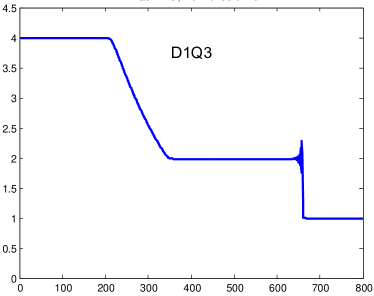
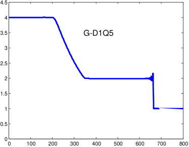
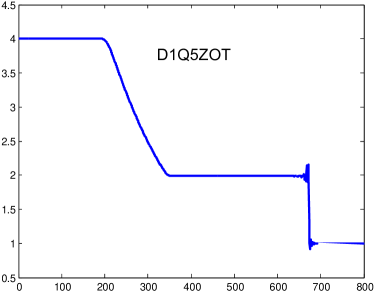
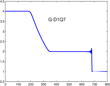
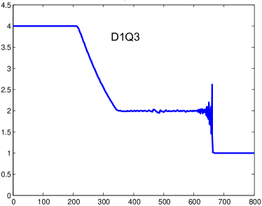
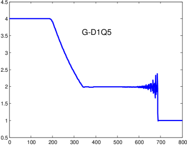
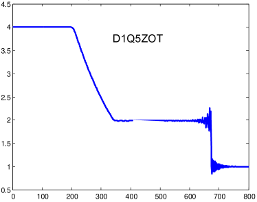
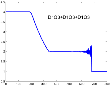
As a benchmark $D1Q5ZOT$ LB model was adopted, this model has good stability [34, 35]. The models were calibrated at the unit temperature $\theta=1$. All the models show good stability for moderate viscosity $\nu\sim 0.1$ ($\nu=\theta\tau$) but show some overrelaxation effects (oscillations) (Fig. 1). When the viscosity was decreased to $0.03$ (this corresponds to the Reynolds number close to $30-40\times 10^{3}$, where the Reynolds number is defined as $uH/\nu$) the oscillations are amplified (Fig. 2). The overall oscillation magnitudes are largest for $D1Q3$, the further small decrease in viscosity leads to breakdown of the solution to $D1Q3$ model while all the other models are able to reproduce the solution (though oscillations are growing). As a result, one can conclude that the models in the hierarchy for $N>1$ have better stability than the conventional $D1Q3$.

Interestingly, that five velocity models for $(-2c,-c,0,c,2c)$ lattice are supposed to be unstable [34, 35]. This result seems to contradict to the presented Sod shock tube simulations since it was shown that the $G$-$D1Q5$ model from the $2N+1,N=2$ hierarchy has good stability. This seeming contradiction has the following explanation. The result in the papers [34, 35] is related to the high order LB model (which exactly reproduces the third order moments of the Maxwell distribution) while in the present case $G$-$D1Q5$ has the same order of isotropy as $D1Q3$ model.

5.2 Knudsen number

For the next two test problems (Couette and Poiseuille flow) the rarefaction measure or Knudsen number should be introduced. The modeling results will be compared with the data from literature in which numerous definitions are used. Thus this definition should be considered in detail for consistency.

Following the paper [8] the viscosity based Knudsen number is introduced

$$k=\frac{\lambda}{H}=\sqrt{\frac{\pi}{2\theta}}\frac{\nu}{H},$$

where $\lambda,H$ are the mean free path and width of the channel for the plane Couette or Poiseuille problem; $\nu=\theta\tau$ is the viscosity, $\tau,\theta$ are the relaxation time and temperature.

In several papers [36, 37, 33] the results for the Poiseuille flow are presented against a rarefaction parameter $\delta$ which is proportional to the inverse of the Knudsen number

$$\delta=\frac{\sqrt{\pi}}{2k},$$

therefore another definition of the Knudsen number can be introduced

$$Kn=\delta^{-1}=\sqrt{\frac{2}{\theta}}\frac{\nu}{H}$$ (14)

In the present paper I will stick to the definition (14) which is most convenient since the benchmark results for the Poiseuille and Couette flows are presented for $\delta$ or $Kn$ [36, 37, 33, 31, 32].

5.3 Couette flow

The plane 2D Couette flow is considered. For this flow the parallel plates move in opposite direction with the velocities $\pm U_{w}$ respectively. The magnitudes of the velocities are taken small, such that the flow velocity is $Ma\sim 10^{-4}$. The kinetic boundary conditions for high-order lattices are stated at the walls [38, 39], $200$ spatial nodes between the walls are used in the computations.

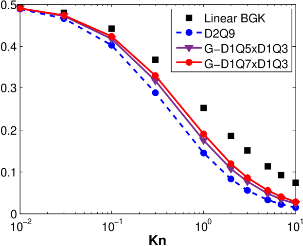
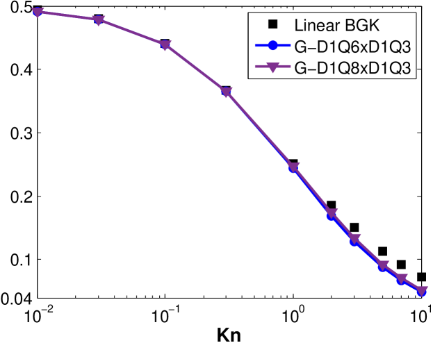
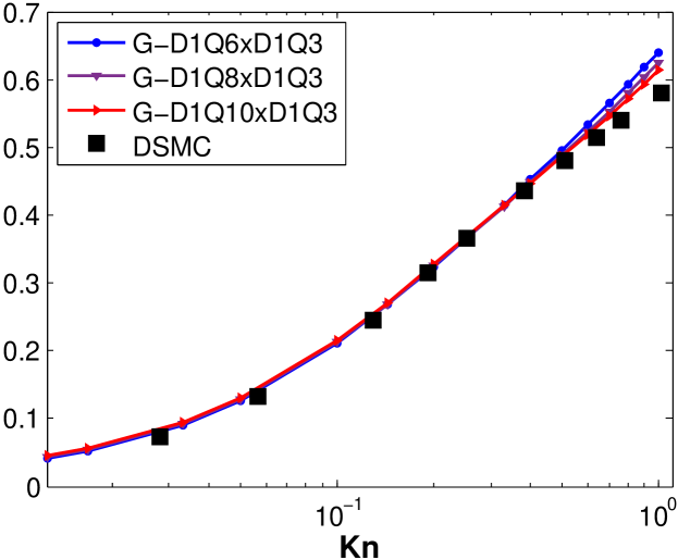
The slip velocities are defined as $u(0)/(2U_{w})$, where $u(0)$ is the velocity at the wall for the LB models. The slip velocities are presented in Fig. 3 and Fig. 4 for the Knudsen numbers varying from $10^{-2}$ to $10^{1}$. The high-precision solutions to the linearized BGK equations are chosen as benchmark [31, 32].

It is worth to mention that for 2D models in the form $G$-$D1Q5\times D1Q3$, $G$-$D1Q7\times D1Q3$ or $G$-$D1Q6\times D1Q3$, $G$-$D1Q8\times D1Q3$ and etc, the parts $G$-$D1Q5$, $G$-$D1Q6$, $G$-$D1Q7$ and etc are responsible for the dynamics transverse to the flow direction (perpendicular to the walls) while the component $D1Q3$ is responsible to the streamwise direction.

Obviously $D2Q9$ fails to reproduce Knudsen layer and understates the slip velocities for $Kn>0.05$. This behavior is well-known [6, 9] and is predicted analytically [6]. The results for the models $G$-$D1Q5\times D1Q3$, $G$-$D1Q7\times D1Q3$ based on the summation procedure presented earlier (1)-(6) are significantly better than $D2Q9$ for all Knudsen numbers. Nevertheless, in comparison with the results for the fourth-order off-lattice $D2Q16$ model (Fig. 1 in the paper [6]) the models $G$-$D1Q5\times D1Q3$, $G$-$D1Q7\times D1Q3$ show worse precision. The model $D2Q16$ predicts Knudsen layer at least qualitatively. Also the lattice velocities for $D2Q16$ model do not have components parallel to the walls. The latter seems to be even more important than the fact that $D2Q16$ is high order LB model. The results for $G$-$D1Q6\times D1Q3$, $G$-$D1Q8\times D1Q3$ models (no lattice velocities parallel to the walls) support this idea. The precision for these models is much better than $G$-$D1Q5\times D1Q3$, $G$-$D1Q7\times D1Q3$ and also $D2Q16$ for all Knudsen numbers (Fig. 4).

The positive effect of zero velocity removal is thoroughly explained in [13, 16]. Zero velocity usually has the lattice weight significantly greater than the weights of the other velocities, on the other hand zero-velocity weight does not influence half-moments (or half-fluxes) which enter the kinetic boundary conditions. Therefore, the wall half-moments are underestimated. The models $G$-$D1Q6\times D1Q3$, $G$-$D1Q8\times D1Q3$ from $(2N+2)$ hierarchy (9)-(12) do not have wall-parallel velocities moreover the form of their local equilibrium is close to Gaussian which result in a good reproduction of the kinetic boundary conditions.

5.4 Poiseuille flow

The force driven 2D Poiseuille flow is considered. The kinetic boundary conditions are stated at two parallel walls [38, 39]. Similarly to the previous case the parts $G$-$D1Q5$, $G$-$D1Q6$, $G$-$D1Q7$ for $G$-$D1Q5\times D1Q3$, $G$-$D1Q6\times D1Q3$, $G$-$D1Q7\times D1Q3$ and etc are responsible for the dynamics transverse to the flow direction (perpendicular to the walls). The force is taken in the linearized form [28]

$$F_{ij}=W_{i}w_{j}c_{j}F,$$

where $i=1\ldots 2N+1$ or $i=1\ldots 2N+2$ and $j=1,2,3$; $F$ is the force amplitude, $W_{i}$ are the weights for the (the values of local equilibrium state taken at $\rho=1,u=0$, see example in Appendix A) for the lattices $G$-$D1Q5$, $G$-$D1Q6$, $G$-$D1Q7$ and etc and $w_{j},c_{j}$ are the weights and the lattice velocities for $D1Q3$ model (calibrated at unit temperature): $(1/6,4/6,1/6)$ and $(-\sqrt{3},0,\sqrt{3})$ respectively; $200$ cross-stream spatial nodes were used in the computations. The amplitude of the force $F$ is taken small such that the flow velocity is of order $Ma^{-4}$, moreover instead of using the force term the boundary conditions with pressure variations were tested [40], they give very similar results to the force-driven case.

The reproduction of the Knudsen paradox i.e. the shape of the the volumetric flow with a minimum near $Kn=1$ is challenging for the Lattice Boltzmann method. The volumetric flow is defined as [8]

$$Q=\frac{\delta}{4U_{0}H}\int_{0}^{H}u(s)ds,$$

where $U_{0}=FH^{2}/(8\rho\nu)$ is the centerline velocity for the Navier-Stokes equation with no-slip boundary conditions, $H$ is the distance between the walls, $\rho$ is the gas density, $\nu$ is the viscosity, $u$ is the streamwise velocity.

The straightforward application of high-order lattices is not sufficient for the reproduction of the rarefied flow effects [41, 13]. For instance, the Knudsen minimum is well reproduced when extreme high-order LB models are used [13]. There exist numerous approaches to improve the results for the Poiseuille flow. The multiple relaxation LB approach is able to capture non-equilibrium rarefaction effects in several test flows [42, 43, 44]. The regularization of LB models significantly improves the results [5, 15] yet the Knudsen minimum is not obtained. The application of the regularization with an additional inclusion of two relaxation times (dependent on Knudsen number) leads to the prediction of the Knudsen minimum [7]. Another solution is the alternation of even and odd high-order LB schemes and averaging the results [45]. The high-order on-lattice models with correct half-fluxes (wall half-moments) [16] show good accuracy for $Kn<1$, the thermal off-lattice schemes with exact half-fluxes based on $S$ kinetic model are able to predict the volumetric flow for a wide range of Knudsen numbers [46, 47, 14].

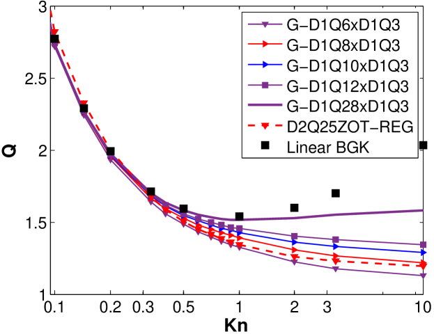
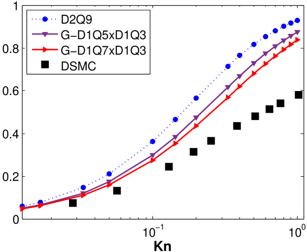
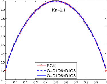
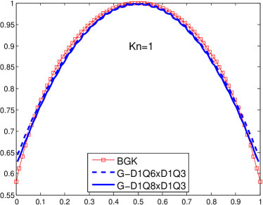
In the present paper un-regularized on-latice LB models with single relaxation time are studied (except the regularized $D2Q25ZOT$ which is used as benchmark). The results for the models from $2N+1$ hierarchy (1)-(6) are presented in Fig.5 and Fig. 7. The precision is significantly increased over $D2Q9$. The volumetric flow modeling results in Fig. 5 can serve as an apparent example of the convergence for the $2N+1$ hierarchy to the BGK equation.

In ballistic regime runaway effects prevent the correct computation of the flux for $2N+1$ hierarchy (1)-(6) while for the models from $2N+2$ hierarchy (9)-(12) runaway effects are absent but the flow does not have minimum. This result is very typical for LB models with a single relaxation time: the models with velocities parallel to the wall suffer from runaway effects, while the models which are free of such lattice velocities do not reproduce the Knudsen minimum, see [8, 48, 15, 16]. Nevertheless, the models from $(2N+2)$ hierarchy (9)-(12) show excellent accuracy in slip and transitional regimes ($Kn<1$), Fig.6, Fig.8 and Fig. 9. The regularized $D2Q25ZOT$ model (2D analog of the regularized $D3Q41$ model applied in [15]) was also implemented for the comparison with the models from $2N+2$ hierarchy. For clarity the volumetric flow is shown in Fig. 6 only for the transitional and ballistic regimes ($Kn\geq 0.1$). All the models have good precision in slip regime only the regularized $D2Q25ZOT$ slightly overestimates the flow. This at least in qualitative agreement with the results from [15], where the slight over prediction of the flow for the regularized $D3Q41$ is observed in the slip and transitional regimes. In the part of the transitional regime and ballistic regime the regularized $D2Q25ZOT$ performs better than $G$-$D1Q6\times D1Q3$, Fig. 6. The next models in the hierarchy $G$-$D1Q8\times D1Q3$, $G$-$D1Q10\times D1Q3$, $G$-$D1Q12\times D1Q3$ surpass both the regularized $D2Q25ZOT$ and $G$-$D1Q6\times D1Q3$ models for all Knudsen numbers and monotonically converge to the BGK model results.

The Knudsen minimum for the even-velocity $2N+2$ hierarchy is observed for $N=10$, and the case $N=13$ i.e. $G$-$D1Q28\times D1Q3$ is presented in Fig. 6. The discrepancy between the model solution and the tabulated data is approximately $10\%$ for the Knudsen numbers in the part of the ballistic regime $1\leq Kn\leq 3.33$. Similar result can be obtained for an even-velocity high-order $D2Q4624$ off-lattice LB model with one relaxation time [13]. In the present case the fully symmetric $2D$ Gaussian LB model for $N=13$ in the $2N+2$ hierarchy has $28*28=784$ velocities ($G$-$D2Q784$). The model $G$-$D2Q784$ is on-lattice and shorter than $D2Q4624$. Therefore, the Gaussian method shows faster convergence to the benchmark results in ballistic regime than the increase of the order for the Gauss-Hermite quadratures in conventional LB models.

6 Conclusion

The new discretization approach for the kinetic BGK model is proposed. This approach somewhat intermediate for the classical LB method and DV approximation of the BGK model. The presented hierarchy of the LB has several attractive properties. The streaming step is linear and the method is conservative, these properties are inherited directly from the conventional LB models. Similarly to the DV methods for the BGK model the errors in the high order moments can be controlled by the choice of the number of the summation steps. Since the shape of the equilibrium state after each summation step approaches closer to the Gauss distribution then the better reproduction of the kinetic boundary conditions is obtained. The numerical experiments for the test problems (2D Couette and Poiseuille flows) support this fact. Moreover, the summation monotonically enlarges the domain of positivity for the local equilibrium state. This results in better stability, though the detailed investigation of stability properties should be performed in future. Finally, applying the Central Limit Theorem several analytical properties are obtained: quadratic convergence to the BGK model and the closed form of the moment generating function.

The presented construction confirms the idea that the precision of LB models (at least in the case of slow test flows) are mostly influenced by the structure of the lattice and the weights but not the order of the lattice [2]. Moreover, the results of the paper give an positive answer on the question of the convergence of the LB method to the BGK model [2, 6]. Interestingly that this convergence is achieved using low-order lattices.

The main drawbacks of the method are the restriction to isothermal flows and cubic growth of the number of lattice velocities for 3D problems. This features are well-known for the conventional LB method and various techniques for overcoming of this difficulties are proposed. These questions are leaved for the future study.

Figure 10: Lattice for $G$-$D1Q5\times D1Q3$ model.

Figure 11: Lattice $G$-$D1Q6\times D1Q3$ model.

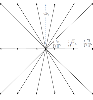
Appendix A $G$-$D1Q5=D1Q3+D1Q3$ example

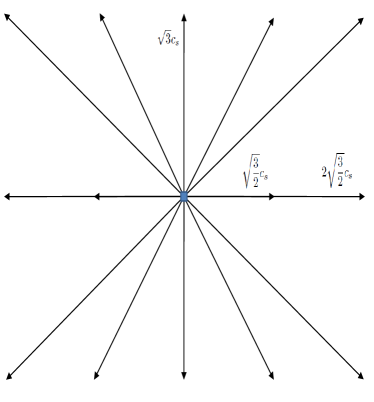
For a particular case of $N=2$ the $G$-$D1Q5$ (the formal sum $D1Q3+D1Q3$) LB model uses $-2c,\,-c,\,0,\,+c,\,+2c$ lattice and the following local equilibrium state is obtained (here the particular case of unit temperature is considered)

$$f_{2}^{eq}(2c)=\rho P_{2,+}^{2},\quad f_{1}^{eq}(c)=2\rho P_{2,0}P_{2,+},$$

$$f_{0}^{eq}(0)=\rho\bigl{(}P_{2,0}^{2}+2P_{2,+}P_{2,-}\bigr{)},$$

$$f_{-1}^{eq}(-c)=2\rho P_{2,0}P_{2,-},\quad f_{-2}^{eq}(-2c)=\rho P_{2,-}^{2},$$

where

$$P_{2,\pm}=\frac{1}{4c^{2}}\left(1\pm cu+\frac{u^{2}}{2}\right),$$

$$P_{2,0}=1-P_{2,+}-P_{2,-},\quad c=\sqrt{3/2}.$$

When the bulk velocity $u$ is zero the total equilibrium state for $D1Q5$ has the following form

$$f_{2}^{eq}(2c)=w_{1}^{2},\quad f_{1}^{eq}(c)=2w_{0}w_{1},$$

$$f_{0}^{eq}(0)=w_{0}^{2}+2w_{1}^{2},$$

$$f_{-1}^{eq}(-c)=2w_{0}w_{1},\quad f_{-2}^{eq}(-2c)=w_{1}^{2},$$

where $w_{0}=4/6,w_{1}=1/6$ are the lattice weights for the $D1Q3$ model. This is the simplest generalization of $D1Q3$ model. It should be mentioned that all the models in the hierarchy have the same order of isotropy (as for $D1Q3$). This is unusual in comparison with the conventional LB method where the increase in number of discrete velocities leads to increase in number of exactly reproduced moments.

Appendix B Third and Fourth moments

Consider the third moment $m_{3}$ for $2N+1$ hierarchy. For the sake of brevity in this Section it is assumed that $\rho=1$. A simplest way to find the moments in an exact form is an application of the moment generating function (8). One has for $2N+1$

$$m_{3}^{(2N+1)}=\frac{d^{3}(P_{N,-}e^{-cs}+P_{N,0}+P_{N,+}e^{cs})^{N}}{ds^{3}}|_{s=0}=$$

$$=N(N-1)(N-2)(P_{N,+}-P_{N,-})^{3}+$$

$$+3N(N-1)(P_{N,+}-P_{N,-})(P_{N,+}+P_{N,-})+N(P_{N,+}-P_{N,-})$$

and remembering the definitions of $P_{N,\pm}$ from (3) the final result is obtained

$$m_{3}^{(2N+1)}=u^{3}+3u\theta_{0}-\frac{u^{3}}{N^{2}},$$

where $\theta_{0}=c_{s}^{2}$ is the gas temperature.

Another way to find this moment is based on the fact that the local equilibrium distribution has the form of the probability density for a sum of the independent and identically distributed random variables, i.e. $Y=\sum_{j}^{N}X_{j}$. Then

$$m_{3}^{(2N+1)}=\langle Y^{3}\rangle=\left\langle\left(\sum_{j=1}^{N}X_{j}\right)^{3}\right\rangle$$

and applying $\langle X_{i}X_{j}X_{k}\rangle=\langle X_{i}\rangle\langle X_{j}\rangle\langle X_{k}\rangle$ if $i\neq j\neq k$ one obtains the expression

$$m_{3}^{(2N+1)}=N(N-1)(N-2)\langle X\rangle^{3}+3N(N-1)\langle X^{2}\rangle\langle X\rangle+N\langle X^{3}\rangle,$$

where $X$ means any of $X_{j}$ . The latter expression leads to the same result.

The fourth moment can be obtained from the moment generating function or by computing $\langle Y^{4}\rangle=\langle(\sum_{j}^{N}X_{j})^{4}\rangle$, after some lengthy algebra one obtains the following result

$$m_{4}^{(2N+1)}=u^{4}+6u^{2}\theta_{0}+3\theta_{0}^{2}+\left(\frac{4}{N^{2}}+\frac{3}{N^{3}}\right)u^{4}-\frac{3\theta_{0}u^{2}}{N^{2}}.$$

For $2N+2$ hierarchy the moment generating function was not obtained, the third moment is then computed in a straightforward way

$$m_{3}^{(2N+2)}=\frac{c^{3}}{2}\sum_{n=-N}^{N}Prob\left(\sum_{j}^{N}X_{j}=nc\right)\times\left(\left(n-\frac{1}{2}\right)^{3}+\left(n+\frac{1}{2}\right)^{3}\right)=$$

$$=\sum_{n=-N}^{N}Prob\left(\sum_{j}^{N}X_{j}=nc\right)(nc)^{3}+\frac{3}{4}c^{2}u.$$

and the sum in the expression above is the third moment for $2N+1$ hierarchy, then

$$m_{3}^{(2N+2)}=u^{3}+3u\left(\theta_{0}+\frac{1}{4}c^{2}\right)-\frac{u^{3}}{N^{2}}$$

finally remembering that the temperature for $2N+2$ hierarchy is given by the relation (13) i.e. equals $\theta_{0}+\frac{c^{2}}{4}$ one can conclude that the error is again $u^{2}/N^{3}$ in comparison with the local Maxwell third moment.

References

- [1] Succi S 2015 EPL 109 50001
- [2] Succi S 2016 AIP Conf. Proc. 1786 030001
- [3] Succi S 2018 The Lattice Boltzmann Equation: For Complex States of Flowing Matter (Oxford: OUP)
- [4] Toschi F and Succi S 2005 Europhys. Lett. 69 549
- [5] Zhang R, Shan X and Chen H 2006 Phys. Rev. E 74 046703
- [6] Ansumali S, Karlin I, Arcidiacono S, Abbas A and Prasianakis N 2007 Phys. Rev. Lett. 98 124502
- [7] Niu X, Hyodo S, Munekata T and Suga K 2007 Phys. Rev. E 76 036711
- [8] Kim S, Pitsch H and Boyd I 2008 J. Comput. Phys. 227 8655
- [9] Tang G, Zhang Y and Emerson D 2008 Phys. Rev. E 77 046701
- [10] Yudistiawan W, Ansumali S and Karlin I 2008 Phys. Rev. E 78 016705
- [11] Verhaeghe F, Luo L and Blanpain B 2009 J. Comput. Phys. 228 147–157
- [12] Yudistiawan W, Kwak S, Patil D and Ansumali S 2010 Phys. Rev. E 82 046701
- [13] Meng J and Zhang Y 2011 Phys. Rev. E 83 036704
- [14] Ambrus V and Sofonea V 2014 Phys. Rev. E 89 041301 (R)
- [15] Montessori A, Prestininzi P, La Rocca M and Succi S 2015 Phys. Rev. E 92 043308
- [16] Feuchter C and Schleifenbaum W 2016 Phys. Rev. E 94 013304
- [17] Silva G and Semiao V 2017 Phys. Rev. E 96 013311
- [18] He X and Luo L 1997 Phys. Rev. E 55 R6333–R6336
- [19] Shan X and He X 1998 Phys. Rev. Lett. 80 65–67
- [20] Shan X, Yuan X and Chen H 2006 J. Fluid Mech. 550 413–441
- [21] Shan X 2010 Phys. Rev. E 81 036702
- [22] Latt J and Chopard B 2006 Math. Comp. Simul. 72 165–168
- [23] Chen H, Zhang R, Staroselsky I and Jhon M 2006 Phys. A 362 125–131
- [24] Mattila K, Philippi P and Hegele Jr L 2017 Phys. Fluids 29 046103
- [25] Montessori A, Falcucci G, Prestininzi P, La Rocca M and Succi S 2014 Phys. Rev. E 89 053317
- [26] Montessori A, La Rocca M, Falcucci G and Succi S 2014 Int. J. Mod. Phys. C 25 1441003
- [27] Mieussens L 2000 Math. Models Meth. Appl. Sci. 10 1121–1149
- [28] Krüger T, Kusumaatmaja H, Kuzmin A, Shardt O, Silva G and Viggen E 2017 The Lattice Boltzmann Method. Principles and Practice (Springer)
- [29] Ferguson T 1996 A Course in Large Sample Theory (Chapman and Hall)
- [30] Karlin I and Asinari P 2010 Physica A 389 1530–1548
- [31] Li W, Luo L and Shen J 2015 Comput. Fluids 111 18
- [32] Jiang S and Luo L 2016 J. Comput. Phys. 316 416
- [33] Cercignani C, Lampis M and Lorenzani S 2004 Phys. Fluids 16 3426
- [34] Chikatamarla S and Karlin I 2006 Phys. Rev. Lett. 97 190601
- [35] Chikatamarla S and Karlin I 2009 Phys. Rev. E 79 046701
- [36] Fukui S and Kaneko R 1990 J. Tribol. 112 78–83
- [37] Sharipov F and Seleznev V 1998 J. Phys. and Chem. Ref. Data 27 657–706
- [38] Meng J and Zhang Y 2014 J. Comput. Phys. 0021-9991 258 601–612
- [39] Ansumali S and Karlin I 2002 Phys. Rev. E 66 026311
- [40] Kim S and Pitsch H 2007 Phys. Fluids 19 108101
- [41] Shi Y, Brookes P, Yap Y and Sader J 2011 Phys. Rev. E 83 045701(R)
- [42] Guo Z, Zheng C and Shi B 2008 Phys. Rev. E 77 036707
- [43] Li Q, He Y, Tang G and Tao W 2011 Microfluidics Nanofluidics 10 607–618
- [44] Su W, Lindsay S, Liu H and Wu L 2017 Phys. Rev. E 96 023309
- [45] de Izarra L, Rouet J and Izrar B 2011 Phys. Rev. E 84 066705
- [46] Ambrus V and Sofonea V 2016 J. Comput. Sci. 17 403––417
- [47] Ambrus V and Sofonea V 2016 J. Comp. Phys. 316 760
- [48] Kim S and Pitsch H 2008 Phys. Rev. E 78 016702