ForestDSH: A Universal Hash Design for Discrete Probability Distributions

Arash Gholami Davoodi, Sean Chang, Hyun Gon Yoo, Anubhav Baweja, Mihir Mongia and Hosein Mohimani
Carnegie Mellon University, Pittsburgh, PA, 15213
Email: {agholami,szchang,hyungony,abaweja,mmongia,hoseinm}@andrew.cmu.edu
Abstract

In this paper, we consider the problem of classification of M𝑀M high dimensional queries y1,,yMSsuperscript𝑦1superscript𝑦𝑀superscript𝑆y^{1},\cdots,y^{M}\in\mathcal{B}^{S} to N𝑁N high dimensional classes x1,,xN𝒜Ssuperscript𝑥1superscript𝑥𝑁superscript𝒜𝑆x^{1},\cdots,x^{N}\in\mathcal{A}^{S} where 𝒜𝒜\mathcal{A} and \mathcal{B} are discrete alphabets and the probabilistic model that relates data to the classes (x,y)𝑥𝑦\mathbb{P}(x,y) is known. This problem has applications in various fields including the database search problem in mass spectrometry. The problem is analogous to the nearest neighbor search problem, where the goal is to find the data point in a database that is the most similar to a query point. The state of the art method for solving an approximate version of the nearest neighbor search problem in high dimensions is locality sensitive hashing (LSH). LSH is based on designing hash functions that map near points to the same buckets with a probability higher than random (far) points. To solve our high dimensional classification problem, we introduce distribution sensitive hashes that map jointly generated pairs (x,y)similar-to𝑥𝑦(x,y)\sim\mathbb{P} to the same bucket with probability higher than random pairs x𝒜similar-to𝑥superscript𝒜x\sim{\mathbb{P}}^{\mathcal{A}} and ysimilar-to𝑦superscripty\sim{\mathbb{P}}^{\mathcal{B}}, where 𝒜superscript𝒜{\mathbb{P}}^{\mathcal{A}} and superscript{\mathbb{P}}^{\mathcal{B}} are the marginal probability distributions of \mathbb{P}. We design distribution sensitive hashes using a forest of decision trees and we show that the complexity of search grows with O(Nλ())𝑂superscript𝑁superscript𝜆O(N^{\lambda^{*}({\mathbb{P}})}) where λ()superscript𝜆\lambda^{*}({\mathbb{P}}) is expressed in an analytical form. We further show that the proposed hashes perform faster than state of the art approximate nearest neighbor search methods for a range of probability distributions, in both theory and simulations. Finally, we apply our method to the spectral library search problem in mass spectrometry, and show that it is an order of magnitude faster than the state of the art methods.

1 Introduction

Consider the problem of classifying a large number of high dimensional data Y={y1,,yM}S𝑌superscript𝑦1superscript𝑦𝑀superscript𝑆Y=\{y^{1},\cdots,y^{M}\}\subset\mathcal{B}^{S} into high dimensional classes X={x1,,xN}𝒜S𝑋superscript𝑥1superscript𝑥𝑁superscript𝒜𝑆X=\{x^{1},\cdots,x^{N}\}\subset\mathcal{A}^{S}, given a known joint probability distribution (x,y)𝑥𝑦\mathbb{P}(x,y), where 𝒜𝒜\mathcal{A} and \mathcal{B} are discrete alphabets. Given a point yY𝑦𝑌y\in Y, the goal is to find the class xX𝑥𝑋x\in X that maximize (yx)conditional𝑦𝑥\mathbb{P}(y\mid x);

ArgmaxxX(yx),𝐴𝑟𝑔subscript𝑥𝑋conditional𝑦𝑥\displaystyle{Arg}\max_{x\in{X}}\mathbb{P}(y\mid x), (1)

where (yx)conditional𝑦𝑥\mathbb{P}(y\mid x) is factorizable to i.i.d. components, i.e.,111Here, we assume that (x)𝑥\mathbb{P}(x) is also factorizable to i.i.d. components.

(yx)=s=1Sp(ysxs).conditional𝑦𝑥superscriptsubscriptproduct𝑠1𝑆𝑝conditionalsubscript𝑦𝑠subscript𝑥𝑠\displaystyle\mathbb{P}(y\mid x)=\prod_{s=1}^{S}p(y_{s}\mid x_{s}). (2)

In this paper, we refer to X={x1,,xN}𝑋superscript𝑥1superscript𝑥𝑁X=\{x^{1},\cdots,x^{N}\} as data base points and Y={y1,,yM}𝑌superscript𝑦1superscript𝑦𝑀Y=\{y^{1},\cdots,y^{M}\} as queries. This problem has application in various fields, including the clustering of spectra generated by mass spectrometry instruments [1]. Consider the problem where there are billions of data points (mass spectra) and given a query spectrum y𝑦y the goal is to find the spectrum x𝑥x that maximize known probability distribution (yx)conditional𝑦𝑥\mathbb{P}(y\mid x) [2, 3]. This is similar to the nearest neighbor search problem [4, 5], where instead of minimizing a distance, we maximize a probability distribution, and has applications in machine learning [6], database querying [7] and computer vision [8, 9] .

A naive approach to solve this problem is to compute (yx)conditional𝑦𝑥\mathbb{P}(y\mid x) for each xX𝑥𝑋x\in X, and find the maximum. The run time for this algorithm is O(NS)𝑂𝑁𝑆O(NS) which is very slow when the number of classes, N𝑁N, is large.

In order to address this problem where the number of classes is massive, multiclass classification methods have been established [10, 11, 12, 13, 14, 15, 16, 17, 18, 19, 20, 21, 22]. For example, in [16] an approach to construct a tree with logarithmic (in terms of number of classes) depth is presented and logarithmic train and test time complexity is achieved. However, these methods are limited to low-dimensional data (when the number of dimensions is less than 101010), and their complexity grows exponentially with the dimension. The methods in [10, 11, 12] speed up the prediction by rejecting a significant portion of classes for each query. However, all these methods suffer from the curse of dimensionality, i.e., when the dimension of the data increases, the complexity of these methods increases linearly with the number of classes.222The curse of dimensionality holds for non-deterministic probability distributions. When p(yx)𝑝conditional𝑦𝑥p(y\mid x) is deterministic, i.e., when it takes only a single value with probability one, there is no curse of dimensionality. In this paper, we are interested in the case of non-deterministic probability distributions. Dimension reduction can also be utilized before applying nearest neighbor search algorithms to high dimensional data [23, 24, 25, 26]. Moreover, Structure Preserving Embedding (SPE) which is a low-dimensional embedding algorithm for Euclidean space is also used as a dimension reduction tool [27]. Set similarity in nearest neighbor search literature is studied extensively [28, 29]. In [28], the authors develop a data structure that solves the problem of approximate set similarity search under Braun-Blanquet similarity B(x,y)=|xy|max(|x|,|y|)𝐵𝑥𝑦𝑥𝑦𝑥𝑦B(x,y)=\frac{|x\cap y|}{\max(|x|,|y|)} in sub-quadratic query time.

A similar problem has been investigated in the field of nearest neighbor search. In this problem, given a set of points in a database, the goal is to find the point in the database that is closest to a query point. A popular approach to this problem is locality sensitive hashing [30, 31]. This approach solves ϵitalic-ϵ\epsilon-approximate nearest neighbor search problem by designing a family of hashes in a way that near points are hashed to the same bucket with probability much higher than random points. In ϵitalic-ϵ\epsilon-approximate nearest neighbor search problem, given a query point y𝑦y, the goal is to find xX𝑥𝑋x\in X for which d(x,y)(1+ϵ)d(x,y)𝑑𝑥𝑦1italic-ϵ𝑑superscript𝑥𝑦d(x,y)\leq(1+\epsilon)d(x^{\prime},y) for all xXsuperscript𝑥𝑋x^{\prime}\in X and X𝑋X is the set of all feasible points [30, 32]. One of the most popular methods for approximate nearest neighbor search is LSH [30, 31, 33, 34, 35, 28]. For any metric space =(M,d)𝑀𝑑\mathcal{M}=(M,d), a family of functions h:S:𝑆h:{\mathcal{M}}\to S is (R,cR,p1,p2)𝑅𝑐𝑅subscript𝑝1subscript𝑝2\mathcal{F}(R,cR,{p}_{1},{p}_{2})-sensitive if for any two points x,y𝑥𝑦x,y\in{\mathcal{M}}:

If d(x,y)R, then h𝒜(x)=h(y) with probability at least p1.formulae-sequenceIf 𝑑𝑥𝑦𝑅 then superscript𝒜𝑥superscript𝑦 with probability at least subscript𝑝1\displaystyle\mbox{If~{}}d(x,y)\leq R,\mbox{~{}then~{}}h^{\mathcal{A}}(x)=h^{\mathcal{B}}(y)\mbox{~{}with probability at least~{}}{p}_{1}. (3)
If d(x,y)cR, then h𝒜(x)=h(y) with probability at most p2.formulae-sequenceIf 𝑑𝑥𝑦𝑐𝑅 then superscript𝒜𝑥superscript𝑦 with probability at most subscript𝑝2\displaystyle\mbox{If~{}}d(x,y)\geq cR,\mbox{~{}then~{}}{h^{\mathcal{A}}(x)}=h^{\mathcal{B}}(y)\mbox{~{}with probability at most~{}}{p}_{2}. (4)

A family is interesting when p1>p2subscript𝑝1subscript𝑝2p_{1}>p_{2}. In the case of hamming distance, i.e., when data are in the form of d𝑑d-dimensional vectors from {0,1}dsuperscript01𝑑{\{0,1\}}^{d}, the family of hashes may be defined simply as H=i=1d{h:{0,1}d{0,1}h(x)=xi}𝐻superscriptsubscript𝑖1𝑑conditional-setsuperscript01𝑑conditional01𝑥subscript𝑥𝑖H=\cup_{i=1}^{d}\{h:\{0,1\}^{d}\to\{0,1\}\mid h(x)=x_{i}\} where xisubscript𝑥𝑖x_{i} is i𝑖i-th coordinate of x𝑥x. From (3) and (4), we conclude that p1=1Rdsubscript𝑝11𝑅𝑑p_{1}=1-\frac{R}{d} and p2=1cRdsubscript𝑝21𝑐𝑅𝑑p_{2}=1-\frac{cR}{d}333Note that d(x,y)R𝑑𝑥𝑦𝑅d(x,y)\leq R is equivalent to x𝑥x and y𝑦y are different in at most R𝑅R coordinates..

In this paper, in addition to going from minimizing a distance to maximizing a probabilistic measure, our approach differs from the classic LSH in the following way. The proposed hashes in this paper are defined to be a subset of integers instead of an integer and our goal is to ensure that444In fact, to control the complexity, two more conditions are defined in Definition 2. (x,y)𝑥𝑦{\mathbb{P}(x,y)} is joint probability distribution while 𝒜(x)superscript𝒜𝑥{\mathbb{P}^{\mathcal{A}}(x)} and (y)superscript𝑦{\mathbb{P}^{\mathcal{B}}(y)} are marginal probability distributions of (x,y)𝑥𝑦{\mathbb{P}(x,y)}. (x,y)𝑥𝑦{\mathbb{Q}(x,y)} is also defined as (x,y)=𝒜(x)(y)𝑥𝑦superscript𝒜𝑥superscript𝑦{\mathbb{Q}(x,y)}={\mathbb{P}^{\mathcal{A}}(x)}{\mathbb{P}^{\mathcal{B}}(y)}.

Prob(H𝒜(x)H(y)(x,y))𝑃𝑟𝑜𝑏superscript𝐻𝒜𝑥superscript𝐻𝑦conditional𝑥𝑦similar-to\displaystyle Prob(H^{\mathcal{A}}(x)\cap H^{\mathcal{B}}(y)\neq\varnothing\mid(x,y)\sim\mathbb{P}) \displaystyle\geq α,𝛼\displaystyle\alpha, (5)
Prob(H𝒜(x)H(y)(x,y))𝑃𝑟𝑜𝑏superscript𝐻𝒜𝑥superscript𝐻𝑦conditional𝑥𝑦similar-to\displaystyle Prob(H^{\mathcal{A}}(x)\cap H^{\mathcal{B}}(y)\neq\varnothing\mid(x,y)\sim\mathbb{Q}) \displaystyle\leq β.𝛽\displaystyle\beta. (6)

In words, these hashes hash the jointly-generated pairs of points to the same buckets with probabilities higher than α𝛼\alpha while hash random pairs of points to the same buckets with probabilities lower than β𝛽\beta. Note that, in this case for data points x𝑥x and y𝑦y, collision happens when we have H𝒜(x)H(y)superscript𝐻𝒜𝑥superscript𝐻𝑦H^{\mathcal{A}}(x)\cap H^{\mathcal{B}}(y)\neq\varnothing, while in the classic LSH, x𝑥x and y𝑦y have collision if H𝒜(x)=H(y)superscript𝐻𝒜𝑥superscript𝐻𝑦H^{\mathcal{A}}(x)=H^{\mathcal{B}}(y). The idea of defining hash collision as the intersection of hash sets has been previously proposed in [28].

Currently, the locality sensitive hashing approach does not generalize to the cases where the triangle inequality, i.e., d(x,y)d(x,z)+d(z,y)𝑑𝑥𝑦𝑑𝑥𝑧𝑑𝑧𝑦d(x,y)\leq d(x,z)+d(z,y) does not hold [29, 30, 31, 36, 37, 38, 39, 40]. These papers are based on balls on some specific points in the metric space and the notion of balls is well defined only for metric spaces that satisfy triangle inequality. Recently, high dimensional approximate nearest neighbors in a known probabilistic distribution setting have been investigated [32, 41]. However, currently it is not possible to design efficient algorithms based on these methods, due to the large number of parameters involved.

The problem of finding high dimensional approximate nearest neighbors in a known probabilistic setting using a bucketing tree algorithm has been studied previously in [41, 42]. Dubiner uses a strategy to hash the data points from an arbitrary joint probability distribution into the leafs of the tree in a way that the paired data collide with a probability higher than the random pairs. Here, paired data refers to pairs coming from joint probability distribution, i.e., (x,y)similar-to𝑥𝑦(x,y)\sim\mathbb{P} random pairs are the pairs coming from an independent probability distribution, i.e., x𝒜similar-to𝑥superscript𝒜x\sim{\mathbb{P}}^{\mathcal{A}} and ysimilar-to𝑦superscripty\sim{\mathbb{P}}^{\mathcal{B}}. However, the algorithm introduced in Dubiner requires solving computationally intractable optimizations, making it impossible to implement (e.g. see equation (126) from [41]). However, in this paper, for the specific case where the distribution for any s{1,2,,S}𝑠12𝑆s\in\{1,2,\cdots,S\} is p(xs=0,ys=0)=p(xs=1,ys=1)=p2,p(xs=1,ys=0)=p(xs=1,ys=0)=1p2formulae-sequence𝑝formulae-sequencesubscript𝑥𝑠0subscript𝑦𝑠0𝑝formulae-sequencesubscript𝑥𝑠1subscript𝑦𝑠1𝑝2𝑝formulae-sequencesubscript𝑥𝑠1subscript𝑦𝑠0𝑝formulae-sequencesubscript𝑥𝑠1subscript𝑦𝑠01𝑝2p(x_{s}=0,y_{s}=0)=p(x_{s}=1,y_{s}=1)=\frac{p}{2},p(x_{s}=1,y_{s}=0)=p(x_{s}=1,y_{s}=0)=\frac{1-p}{2}, our theoretical and practical results are compared to [41] for the range of 0p10𝑝10\leq p\leq 1.

In this paper, we propose to solve (1) by defining a family of distribution sensitive hashes satisfying the following property. They hash the jointly-generated pairs of points to the same buckets with probabilities much higher than random pairs. We further design an algorithm to solve (1) in sub-linear time using these families of hashes. Next, a method to find optimal family of hashes is presented to achieve minimum search complexity using multiple decision trees. Note that, these decision trees have the same tree structure while they apply to different permutations {1,2,,S}{1,2,,S}12𝑆12𝑆\{1,2,\cdots,S\}\rightarrow\{1,2,\cdots,S\} of the data. This way, we design forest of decision trees where each decision tree captures a very small ratio α𝛼\alpha of true pairs for some α+𝛼superscript\alpha\in\mathbb{R}^{+} and by recruiting #bands=O(1α)#𝑏𝑎𝑛𝑑𝑠𝑂1𝛼\#bands=O(\frac{1}{\alpha}) independently permuted decision trees we can reach near perfect recovery of all the true pairs. In this paper, we refer to each decision tree as a band and #bands#𝑏𝑎𝑛𝑑𝑠\#bands is referred to as the number of bands.

The main idea is that we construct decision-tree hashes, in a way that the chance of true pairs hashing to the same leaf nodes in these decision trees is higher than random points (Figure 111). The decision tree is built in a way that the ratio (x,y)(x,y)𝑥𝑦𝑥𝑦\frac{\mathbb{P}(x,y)}{\mathbb{Q}(x,y)} is higher than a minimum threshold, while the ratios (x,y)𝒜(x)𝑥𝑦superscript𝒜𝑥\frac{\mathbb{P}(x,y)}{\mathbb{P}^{\mathcal{A}}(x)} and (x,y)(y)𝑥𝑦superscript𝑦\frac{\mathbb{P}(x,y)}{\mathbb{P}^{\mathcal{B}}(y)} and the number of nodes in the graph are lower than a maximum thresholds, see Algorithm 4. We further determined the optimal tree among many trees that can be constructed in this way. Two theorems are presented here on the complexity of the decision tree built in Algorithm 4.

  1. 1.

    No decision tree exists with the overall search complexity below O(Nλ)𝑂superscript𝑁superscript𝜆O(N^{\lambda^{*}}) where λsuperscript𝜆\lambda^{*} is derived analytically from the probability distribution (x,y)𝑥𝑦\mathbb{P}(x,y).

  2. 2.

    The decision tree construction of Algorithm 4 described in (57) results in the overall search with complexity O(Nλ)𝑂superscript𝑁superscript𝜆O(N^{\lambda^{*}}).

Our results show that our approach, Forest-wise distribution sensitive hashing (ForestDSH), provides a universal hash design for arbitrary discrete joint probability distributions, outperforming the existing state of the art approaches in specific range of distributions, in theory and practice. Moreover, we applied this method to the problem of clustering spectra generated from mass spectrometry instruments.

An alternative strategy for solving (2) is to reformulate the problem as minimum inner product search problem (MIPS) [35] by transferring the data points into a new space. However, as we show in Section 6 the transferred data points are nearly orthogonal to each other making it very slow to find maximum inner product using the existing method [35].

Note that, the algorithms presented in this paper are based on the assumption that the true pairs are generated from a known distribution \mathbb{P}. The distribution \mathbb{P} can be learned from a training dataset of true pairs. In practice, training data can be collected by running a brute force search on smaller data sets or portion of the whole data. For example, in case of mass spectrometry search, we collect training data by running brute-force search on small portion of our data [1]. Note that, we can never perfectly learn the probability distribution that the data is generated from. In Theorem 3, we prove that our algorithm is robust to noise and our experiment confirms this.

Notation: The cardinality of a set A𝐴A is denoted as |A|𝐴|A|. The sets \mathbb{N} and \mathbb{R} stand for the sets of natural and real numbers, respectively. We use ()\mathbb{P}(\cdot) and ()\mathbb{Q}(\cdot) to denote the probability function Prob()Prob\mbox{Prob}(\cdot). 𝔼(ν)𝔼𝜈\mathbb{E}(\nu) denotes the expected value of the random variable v𝑣v. Moreover, we use the notation f(x)=O(g(x))𝑓𝑥𝑂𝑔𝑥f(x)=O(g(x)), if lim supx|f(x)|g(x)<subscriptlimit-supremum𝑥𝑓𝑥𝑔𝑥\limsup_{x\rightarrow\infty}\frac{|f(x)|}{g(x)}<\infty and the notation f(x)=Ω(g(x))𝑓𝑥Ω𝑔𝑥f(x)=\Omega(g(x)), if lim supx|f(x)|g(x)>0subscriptlimit-supremum𝑥𝑓𝑥𝑔𝑥0\limsup_{x\rightarrow\infty}\frac{|f(x)|}{g(x)}>0. In this paper, logx𝑥\log x is computed to the base e𝑒e.

2 Definitions

Definition 1

Define the S𝑆S-dimensional joint probability distribution \mathbb{P} as follows.

:𝒜S×S[0,1],:superscript𝒜𝑆superscript𝑆01\displaystyle\mathbb{P}:\mathcal{A}^{S}\times\mathcal{B}^{S}\rightarrow[0,1], (x,y)=s=1Sp(xs,ys),𝑥𝑦superscriptsubscriptproduct𝑠1𝑆𝑝subscript𝑥𝑠subscript𝑦𝑠\displaystyle\mathbb{P}(x,y)=\prod_{s=1}^{S}{p}(x_{s},y_{s}), (7)

where 𝒜={a1,a2,,ak}𝒜subscript𝑎1subscript𝑎2subscript𝑎𝑘\mathcal{A}=\{a_{1},a_{2},\cdots,a_{k}\}, ={b1,b2,,bl}subscript𝑏1subscript𝑏2subscript𝑏𝑙\mathcal{B}=\{b_{1},b_{2},\cdots,b_{l}\}, x=(x1,x2,,xS)𝒜S𝑥subscript𝑥1subscript𝑥2subscript𝑥𝑆superscript𝒜𝑆x=(x_{1},x_{2},\cdots,x_{S})\in\mathcal{A}^{S} and y=(y1,y2,,yS)S𝑦subscript𝑦1subscript𝑦2subscript𝑦𝑆superscript𝑆y=(y_{1},y_{2},\cdots,y_{S})\in\mathcal{B}^{S} where k,l<𝑘𝑙k,l<\infty. On the other hand, we assume that the probability distribution function p(a,b)𝑝𝑎𝑏{p}(a,b) is independent of s𝑠s and satisfies a[k],b[l]pa,b=1subscriptformulae-sequence𝑎delimited-[]𝑘𝑏delimited-[]𝑙subscript𝑝𝑎𝑏1\sum_{a\in[k],b\in[l]}p_{a,b}=1. Similarly, we define the marginal probability distributions 𝒜:𝒜S[0,1]:superscript𝒜superscript𝒜𝑆01\mathbb{P}^{\mathcal{A}}:\mathcal{A}^{S}\rightarrow[0,1], :S[0,1]:superscriptsuperscript𝑆01\mathbb{P}^{\mathcal{B}}:\mathcal{B}^{S}\rightarrow[0,1] and :𝒜S×S[0,1]:superscript𝒜𝑆superscript𝑆01\mathbb{Q}:\mathcal{A}^{S}\times\mathcal{B}^{S}\rightarrow[0,1] as 𝒜(x)=s=1Sp𝒜(xs)superscript𝒜𝑥superscriptsubscriptproduct𝑠1𝑆superscript𝑝𝒜subscript𝑥𝑠\mathbb{P}^{\mathcal{A}}(x)=\prod_{s=1}^{S}{p}^{\mathcal{A}}(x_{s}), (y)=s=1Sp(ys)superscript𝑦superscriptsubscriptproduct𝑠1𝑆superscript𝑝subscript𝑦𝑠\mathbb{P}^{\mathcal{B}}(y)=\prod_{s=1}^{S}{p}^{\mathcal{B}}(y_{s}) and (x,y)=s=1Sq(xs,ys)𝑥𝑦superscriptsubscriptproduct𝑠1𝑆𝑞subscript𝑥𝑠subscript𝑦𝑠\mathbb{Q}(x,y)=\prod_{s=1}^{S}{q}(x_{s},y_{s}), where

p𝒜(xs)superscript𝑝𝒜subscript𝑥𝑠\displaystyle{p}^{\mathcal{A}}(x_{s}) =\displaystyle= j=1lp(xs,bj),superscriptsubscript𝑗1𝑙𝑝subscript𝑥𝑠subscript𝑏𝑗\displaystyle\sum_{j=1}^{l}p(x_{s},b_{j}), (8)
p(ys)superscript𝑝subscript𝑦𝑠\displaystyle{p}^{\mathcal{B}}(y_{s}) =\displaystyle= i=1kp(ai,ys),superscriptsubscript𝑖1𝑘𝑝subscript𝑎𝑖subscript𝑦𝑠\displaystyle\sum_{i=1}^{k}p(a_{i},y_{s}), (9)
q(xs,ys)𝑞subscript𝑥𝑠subscript𝑦𝑠\displaystyle{q}(x_{s},y_{s}) =\displaystyle= p𝒜(xs)×p(ys).superscript𝑝𝒜subscript𝑥𝑠superscript𝑝subscript𝑦𝑠\displaystyle{p}^{\mathcal{A}}(x_{s})\times{p}^{\mathcal{B}}(y_{s}). (10)

We use pijsubscript𝑝𝑖𝑗p_{ij} instead of p(ai,bj)𝑝subscript𝑎𝑖subscript𝑏𝑗p(a_{i},b_{j}) for simplicity. Moreover, pi𝒜superscriptsubscript𝑝𝑖𝒜p_{i}^{\mathcal{A}}, pjsuperscriptsubscript𝑝𝑗p_{j}^{\mathcal{B}} and qijsubscript𝑞𝑖𝑗q_{ij} are defined as j=1lpijsuperscriptsubscript𝑗1𝑙subscript𝑝𝑖𝑗\sum_{j=1}^{l}p_{ij}, i=1kpijsuperscriptsubscript𝑖1𝑘subscript𝑝𝑖𝑗\sum_{i=1}^{k}p_{ij} and q(ai,bj)𝑞subscript𝑎𝑖subscript𝑏𝑗q(a_{i},b_{j}), respectively. Finally, we use compact notations P=[pij]𝑃delimited-[]subscript𝑝𝑖𝑗P=[p_{ij}] and Q=[qij]𝑄delimited-[]subscript𝑞𝑖𝑗Q=[q_{ij}] as the k×l𝑘𝑙k\times l matrices with pijsubscript𝑝𝑖𝑗p_{ij} and qijsubscript𝑞𝑖𝑗q_{ij} in their i𝑖i-th row and j𝑗j-th column, respectively.

We define family of distribution sensitive hashes as follows.

Definition 2

[Family of Distribution Sensitive Hashes] Assume that the four parameters α𝛼\alpha, β𝛽\beta, γ𝒜superscript𝛾𝒜\gamma^{\mathcal{A}} and γsuperscript𝛾\gamma^{\mathcal{B}} along with the probability distributions \mathbb{P}, 𝒜superscript𝒜\mathbb{P}^{\mathcal{A}}, superscript\mathbb{P}^{\mathcal{B}}, \mathbb{Q} and finite set VBucketssubscript𝑉𝐵𝑢𝑐𝑘𝑒𝑡𝑠V_{Buckets} are given where 𝒜superscript𝒜\mathbb{P}^{\mathcal{A}} and superscript\mathbb{P}^{\mathcal{B}} are marginal distributions of \mathbb{P} and =𝒜superscript𝒜superscript\mathbb{Q}=\mathbb{P}^{\mathcal{A}}\mathbb{P}^{\mathcal{B}}. A family of hashes Hz𝒜:𝒜S2VBuckets:superscriptsubscript𝐻𝑧𝒜superscript𝒜𝑆superscript2subscript𝑉𝐵𝑢𝑐𝑘𝑒𝑡𝑠H_{z}^{\mathcal{A}}:\mathcal{A}^{S}\rightarrow 2^{V_{Buckets}} and Hz:S2VBuckets:superscriptsubscript𝐻𝑧superscript𝑆superscript2subscript𝑉𝐵𝑢𝑐𝑘𝑒𝑡𝑠H_{z}^{\mathcal{B}}:\mathcal{B}^{S}\rightarrow 2^{V_{Buckets}} is called (,α,β,γ𝒜,γ)𝛼𝛽superscript𝛾𝒜superscript𝛾(\mathbb{P},\alpha,\beta,\gamma^{\mathcal{A}},\gamma^{\mathcal{B}})-distribution sensitive, if the following hold

α𝛼\displaystyle\alpha =\displaystyle= vVBucketsProb(vHz𝒜(x)Hz(y)(x,y)),subscript𝑣subscript𝑉𝐵𝑢𝑐𝑘𝑒𝑡𝑠𝑃𝑟𝑜𝑏𝑣superscriptsubscript𝐻𝑧𝒜𝑥conditionalsuperscriptsubscript𝐻𝑧𝑦𝑥𝑦similar-to\displaystyle\sum_{v\in V_{Buckets}}Prob(v\in H_{z}^{\mathcal{A}}(x)\cap H_{z}^{\mathcal{B}}(y)\mid(x,y)\sim\mathbb{P}), (11)
β𝛽\displaystyle\beta =\displaystyle= vVBucketsProb(vHz𝒜(x)Hz(y)(x,y)),subscript𝑣subscript𝑉𝐵𝑢𝑐𝑘𝑒𝑡𝑠𝑃𝑟𝑜𝑏𝑣superscriptsubscript𝐻𝑧𝒜𝑥conditionalsuperscriptsubscript𝐻𝑧𝑦𝑥𝑦similar-to\displaystyle\sum_{v\in V_{Buckets}}Prob(v\in H_{z}^{\mathcal{A}}(x)\cap H_{z}^{\mathcal{B}}(y)\mid(x,y)\sim\mathbb{Q}), (12)
γ𝒜superscript𝛾𝒜\displaystyle\gamma^{\mathcal{A}} =\displaystyle= vVBucketsProb(vHz𝒜(x)x𝒜),subscript𝑣subscript𝑉𝐵𝑢𝑐𝑘𝑒𝑡𝑠𝑃𝑟𝑜𝑏𝑣conditionalsuperscriptsubscript𝐻𝑧𝒜𝑥𝑥similar-tosuperscript𝒜\displaystyle\sum_{v\in V_{Buckets}}Prob(v\in H_{z}^{\mathcal{A}}(x)\mid x\sim\mathbb{P}^{\mathcal{A}}), (13)
γsuperscript𝛾\displaystyle\gamma^{\mathcal{B}} =\displaystyle= vVBucketsProb(vHz(y)y),subscript𝑣subscript𝑉𝐵𝑢𝑐𝑘𝑒𝑡𝑠𝑃𝑟𝑜𝑏𝑣conditionalsuperscriptsubscript𝐻𝑧𝑦𝑦similar-tosuperscript\displaystyle\sum_{v\in V_{Buckets}}Prob(v\in H_{z}^{\mathcal{B}}(y)\mid y\sim\mathbb{P}^{\mathcal{B}}), (15)
Hz𝒜(x)Hz(y)1,delimited-∣∣superscriptsubscript𝐻𝑧𝒜𝑥superscriptsubscript𝐻𝑧𝑦1\displaystyle{\mid H_{z}^{\mathcal{A}}(x)\cap H_{z}^{\mathcal{B}}(y)\mid}\leq 1,

where 1z#bands1𝑧#𝑏𝑎𝑛𝑑𝑠1\leq z\leq\#bands and #bands#𝑏𝑎𝑛𝑑𝑠\#bands represent the number of bands, while VBucketssubscript𝑉𝐵𝑢𝑐𝑘𝑒𝑡𝑠V_{Buckets} represent a set of indices for the buckets. We show how to choose #bands#𝑏𝑎𝑛𝑑𝑠\#bands in (51) in Appendix C and how to select VBucketssubscript𝑉𝐵𝑢𝑐𝑘𝑒𝑡𝑠V_{Buckets} in Algorithm 3. Intuitively, α𝛼\alpha represents the chance of a true pair falling in the same bucket, while β𝛽\beta represents the chance of random pairs falling in the same bucket. We will show that γ𝒜superscript𝛾𝒜\gamma^{\mathcal{A}} and γsuperscript𝛾\gamma^{\mathcal{B}} represent the complexity of computing which buckets the data points fall into. In the next section, we will describe how the families of distribution sensitive hashes can be used to design an efficient solution for (1). Note that, in [28] definitions similar to Definition 2 have been made in order to speed up set similarity search. How the data points are mapped through a decision tree is sketched in Figure 1. The decision tree and the set of buckets are explained in Algorithm 4. Finally, in Figure 2, we show how the rates of positive call for true and random pairs, i.e., α𝛼\alpha and β𝛽\beta are derived. The average number of times that data points and queries fall in buckets, i.e., γ𝒜superscript𝛾𝒜\gamma^{\mathcal{A}} and γsuperscript𝛾\gamma^{\mathcal{B}} are also derived and shown in this figure.

Remark 1

In classic LSH, we have |H𝒜(x)|=1superscript𝐻𝒜𝑥1|H^{\mathcal{A}}(x)|=1 and |H(y)|=1superscript𝐻𝑦1|H^{\mathcal{B}}(y)|=1. Therefore, γ𝒜=γ=1superscript𝛾𝒜superscript𝛾1\gamma^{\mathcal{A}}=\gamma^{\mathcal{B}}=1. Our approach is more flexible in the following two ways. First, we allow for γ𝒜superscript𝛾𝒜\gamma^{\mathcal{A}} and γsuperscript𝛾\gamma^{\mathcal{B}} to be larger than one. Moreover, even in the case of γ𝒜=γ=1superscript𝛾𝒜superscript𝛾1\gamma^{\mathcal{A}}=\gamma^{\mathcal{B}}=1, our method can optimize over the larger set of possible hashes.
Refer to caption

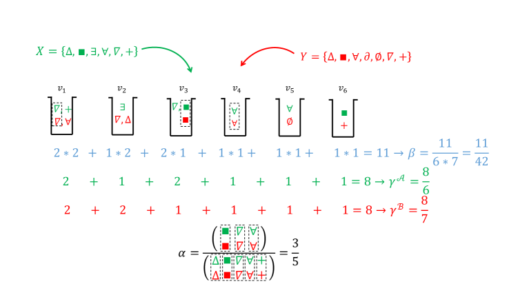
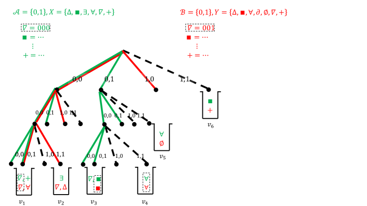
Figure 1: Distribution sensitive hashing is based on a decision tree G𝐺G and a set of buckets VBucketssubscript𝑉𝐵𝑢𝑐𝑘𝑒𝑡𝑠V_{Buckets} which are a subset of leaf nodes of G𝐺G. Construction of the tree and VBucketssubscript𝑉𝐵𝑢𝑐𝑘𝑒𝑡𝑠V_{Buckets} are explained in Algorithm 4. Here, VBucketssubscript𝑉𝐵𝑢𝑐𝑘𝑒𝑡𝑠V_{Buckets} has six buckets in it. We map data points to buckets by propagating them down the tree, starting from the root using Algorithm 3. If we reach a bucket node, we insert the data point. On the other hand, only a subset of leaf nodes are labeled as bucket and if we reach a leaf node that is not a bucket node, we will simply ignore it. The mapping of =000000\triangledown=000 and =001001\triangledown=001 are shown in the figure for S=3𝑆3S=3. Each of the data points =001001\triangledown=001 and =000000\triangledown=000 are mapped to two buckets. Consider data point =000000\triangledown=000. Mapping this point by propagating down the tree, we end up with the two buckets v1subscript𝑣1v_{1} and v3subscript𝑣3v_{3}. Note that, the first character on each of the edges in the paths from root to v1subscript𝑣1v_{1} and v3subscript𝑣3v_{3} is 00. Similarly mapping =001001\triangledown=001 by propagating down the tree, we end up with the two buckets v1subscript𝑣1v_{1} and v2subscript𝑣2v_{2} as the second alphabet on the edges should be 00 in all the first two depths and 111 at the third depth.

Refer to caption

Figure 2: For the data points that are mapped to each bucket, we call them positive (see Algorithm 2). The rate of positive call for true and random pairs are shown as α𝛼\alpha and β𝛽\beta. The average number of times x𝑥x and y𝑦y data points appear in buckets are also shown as γ𝒜superscript𝛾𝒜\gamma^{\mathcal{A}} and γsuperscript𝛾\gamma^{\mathcal{B}}. For formal definition of α𝛼\alpha, β𝛽\beta, γ𝒜superscript𝛾𝒜\gamma^{\mathcal{A}} and γsuperscript𝛾\gamma^{\mathcal{B}}, see Definition 2. Here, we derive the empirical probabilities ((11)(15))italic-(11italic-)italic-(15italic-)(\eqref{family1}-\eqref{family2}) in Definition 2. For example, β𝛽\beta is derived by counting the number of data points combinations in all the six buckets, i.e., 22+12+21+11+11+112212211111112*2+1*2+2*1+1*1+1*1+1*1 over all the possible number of data points which is 67676*7. Here the size of X𝑋X is six, and the size of Y𝑌Y is 7. Similarly, γ𝒜superscript𝛾𝒜\gamma^{\mathcal{A}} is derived by counting number of data points from the set X𝑋X designated to the buckets divided by |X|𝑋|X|.

Here we present a general algorithm on how ForestDSH algorithm works.

Algorithm 1 ForestDSH
  Inputs: Probability distribution \mathbb{P}, X={x1,,xN}𝒜S𝑋superscript𝑥1superscript𝑥𝑁superscript𝒜𝑆{X}=\{x^{1},\cdots,x^{N}\}\subset\mathcal{A}^{S}, yS𝑦superscript𝑆y\in\mathcal{B}^{S}, true positive rate TP𝑇𝑃TP and threshold ΔΔ\Delta.
  Output: Classes xX𝑥𝑋x\in{X} satisfying P(yx)>Δ𝑃conditional𝑦𝑥ΔP(y\mid x)>\Delta.
  procedure:
  Run Algorithm 5.
        This algorithm takes probability distribution \mathbb{P}, M𝑀M and N𝑁N as inputs and generates parameters for decision tree design such as μsuperscript𝜇\mu^{*}, νsuperscript𝜈\nu^{*}, ηsuperscript𝜂\eta^{*}, λsuperscript𝜆\lambda^{*}, and δ𝛿\delta.
  Run Algorithm 4.
        Here, the parameters generated in Algorithm 5 are given as an input while it gives G=(V,E,f)𝐺𝑉𝐸𝑓G=(V,E,f) and a subset of leaf nodes of the decision tree VBucketssubscript𝑉𝐵𝑢𝑐𝑘𝑒𝑡𝑠V_{Buckets} as outputs.
  Run Algorithm 3.
        In this algorithm, list of buckets VBucketssubscript𝑉𝐵𝑢𝑐𝑘𝑒𝑡𝑠V_{Buckets}, permutations permz,1z#bands𝑝𝑒𝑟subscript𝑚𝑧1𝑧#𝑏𝑎𝑛𝑑𝑠perm_{z},1\leq z\leq\#bands, and a set of data points X={x1,,xN}𝑋superscript𝑥1superscript𝑥𝑁X=\{x^{1},\cdots,x^{N}\} are given as input while the outputs are Hz𝒜(x)superscriptsubscript𝐻𝑧𝒜𝑥H_{z}^{\mathcal{A}}(x) for each xX𝑥𝑋x\in X and each band 1z#bands1𝑧#𝑏𝑎𝑛𝑑𝑠1\leq z\leq\#bands. Similarly, Hz(y)superscriptsubscript𝐻𝑧𝑦H_{z}^{\mathcal{B}}(y) are derived from this algorithm
  Run Algorithm 2.
        This algorithm takes X={x1,,xN}𝒜S𝑋superscript𝑥1superscript𝑥𝑁superscript𝒜𝑆{X}=\{x^{1},\cdots,x^{N}\}\subset\mathcal{A}^{S}, yS𝑦superscript𝑆y\in\mathcal{B}^{S}, #bands,VBuckets,Hz𝒜(x),Hz(y)#𝑏𝑎𝑛𝑑𝑠subscript𝑉𝐵𝑢𝑐𝑘𝑒𝑡𝑠superscriptsubscript𝐻𝑧𝒜𝑥superscriptsubscript𝐻𝑧𝑦\#bands,V_{Buckets},H_{z}^{\mathcal{A}}(x),H_{z}^{\mathcal{B}}(y) and threshold ΔΔ\Delta as an input and gives Classes xX𝑥𝑋x\in X satisfying P(yx)>Δ𝑃conditional𝑦𝑥ΔP(y\mid x)>\Delta as an output.

3 Forest Distribution Sensitive Hashing Algorithm

In this section, we assume an oracle has given us a family of distribution sensitive hashes Hz𝒜,Hz,z:1z#bands:superscriptsubscript𝐻𝑧𝒜superscriptsubscript𝐻𝑧for-all𝑧1𝑧#𝑏𝑎𝑛𝑑𝑠H_{z}^{\mathcal{A}},H_{z}^{\mathcal{B}},\forall z:1\leq z\leq\#bands that satisfies ((11)(15))italic-(11italic-)italic-(15italic-)(\eqref{family1}-\eqref{family5}). Inspired by LSH method, we present Algorithm 2 for solving (1) using this family.

Algorithm 2 Solving maximum likelihood classification (1) by ForestDSH
  Inputs: X={x1,,xN}𝒜S𝑋superscript𝑥1superscript𝑥𝑁superscript𝒜𝑆{X}=\{x^{1},\cdots,x^{N}\}\subset\mathcal{A}^{S}, yS𝑦superscript𝑆y\in\mathcal{B}^{S}, #bands,VBuckets,Hz𝒜(x),Hz(y)#𝑏𝑎𝑛𝑑𝑠subscript𝑉𝐵𝑢𝑐𝑘𝑒𝑡𝑠superscriptsubscript𝐻𝑧𝒜𝑥superscriptsubscript𝐻𝑧𝑦\#bands,V_{Buckets},H_{z}^{\mathcal{A}}(x),H_{z}^{\mathcal{B}}(y) and threshold ΔΔ\Delta.
  Output: Classes xX𝑥𝑋x\in{X} satisfying P(yx)>Δ𝑃conditional𝑦𝑥ΔP(y\mid x)>\Delta.
  For z{1,2,,#bands}𝑧12#𝑏𝑎𝑛𝑑𝑠z\in\{1,2,\cdots,\#bands\}
         For vVBuckets𝑣subscript𝑉𝐵𝑢𝑐𝑘𝑒𝑡𝑠v\in V_{Buckets}
             For {xXvHz𝒜(x)}conditional-set𝑥𝑋𝑣superscriptsubscript𝐻𝑧𝒜𝑥\{x\in X\mid v\in H_{z}^{\mathcal{A}}(x)\}
                 If vHz(y)𝑣superscriptsubscript𝐻𝑧𝑦v\in H_{z}^{\mathcal{B}}(y)
                        Call (x,y)𝑥𝑦(x,y) a positive, compute (yx)conditional𝑦𝑥\mathbb{P}(y\mid x) and report x𝑥x if (yx)>Δconditional𝑦𝑥Δ\mathbb{P}(y\mid x)>\Delta.
Remark 2

Note that, the number of times (yx)conditional𝑦𝑥\mathbb{P}(y\mid x) is computed in the brute force method to solve (1) is |X|𝑋|X|. Note that, in the optimization problem (1), the point yY𝑦𝑌y\in Y is given. The goal of Algorithm 2 is to solve (1) with a much smaller number of comparisons than the brute force.

Remark 3

In the special case when the hashes are coming from a decision tree, we analyze the complexity of Algorithm 2 in Section 5. We show that the number of positive calls in Algorithm 2 is proportional to β𝛽\beta, while the complexity of computing |Hz𝒜(x)|superscriptsubscript𝐻𝑧𝒜𝑥|H_{z}^{\mathcal{A}}(x)| and |Hz(y)|superscriptsubscript𝐻𝑧𝑦|H_{z}^{\mathcal{B}}(y)| are proportional to γ𝒜superscript𝛾𝒜\gamma^{\mathcal{A}} and γsuperscript𝛾\gamma^{\mathcal{B}}. Moreover, the chance of true pairs being called positive grows with α𝛼\alpha. Therefore, in the next sections, we attempt to design buckets such that α𝛼\alpha is maximized, while β𝛽\beta, γ𝒜superscript𝛾𝒜\gamma^{\mathcal{A}} and γsuperscript𝛾\gamma^{\mathcal{B}} are minimized.

Now, the question is how we can design these families in a way to minimize the complexity, and efficiently map data points to these families. We investigate these questions in Sections 4 and 4.1.

4 Designing ForestDSH Using a Decision Tree Structure

In the previous section, we assumed that an oracle has given us a family of distribution sensitive hashes. In this section, we design buckets that satisfy ((11)(15))italic-(11italic-)italic-(15italic-)(\eqref{family1}-\eqref{family5}) using a forest of decision trees with the same structure. Here, we focus on the probability distributions that can be factorized as the product of i.i.d. components.

Each of our decision trees recovers ratio α𝛼\alpha of true pairs and by recruiting #bands=O(1α)#𝑏𝑎𝑛𝑑𝑠𝑂1𝛼\#bands=O(\frac{1}{\alpha}) decision trees we can recover nearly all true pairs. This can be more efficient than using a single decision tree classifier as achieving near perfect true pair recovery by the single decision tree would require near brute-force complexity. By allowing α<1𝛼1\alpha<1, we can select decision tree that avoid paths with low (x,y)𝑥𝑦\mathbb{P}(x,y) resulting in complexities much lower than the brute-force search. Note that α𝛼\alpha is the true positive rate, e.g. the probability that a true pair (x,y)𝑥𝑦(x,y) fall in the same bucket, therefore we always have α1𝛼1\alpha\leq 1, see Figure 2.

Assume that a decision tree G=(V,E,f)𝐺𝑉𝐸𝑓G=(V,E,f) is given where V𝑉V is the set of nodes, E𝐸E is the set of edges, VlVsubscript𝑉𝑙𝑉V_{l}\subset V is the set of leaf nodes in the decision tree and f:V/Vl×𝒜×V:𝑓𝑉subscript𝑉𝑙𝒜𝑉f:V/V_{l}\times\mathcal{A}\times\mathcal{B}\rightarrow V is the decision function, see Figure 1. For the two nodes v1,v2Vsubscript𝑣1subscript𝑣2𝑉v_{1},v_{2}\in V, v1subscript𝑣1v_{1} is called an ancestor of v2subscript𝑣2v_{2} if v1subscript𝑣1v_{1} falls within the path from v2subscript𝑣2v_{2} to root. In this case, v2subscript𝑣2v_{2} is called a descendant of v1subscript𝑣1v_{1}. Furthermore, assume that a subset of leaf nodes VBucketsVlsubscript𝑉𝐵𝑢𝑐𝑘𝑒𝑡𝑠subscript𝑉𝑙V_{Buckets}\subset V_{l} is given and at depth s𝑠s in the decision tree, the decisions depend only on xssubscript𝑥𝑠x_{s} and yssubscript𝑦𝑠y_{s} where x=(x1,,xS)𝑥subscript𝑥1subscript𝑥𝑆x=(x_{1},\cdots,x_{S}) and y=(y1,,yS)𝑦subscript𝑦1subscript𝑦𝑆y=(y_{1},\cdots,y_{S}) are S𝑆S-dimensional data point and query, respectively. We define functions Seq𝒜:Vs=0S𝒜s:𝑆𝑒superscript𝑞𝒜𝑉superscriptsubscript𝑠0𝑆superscript𝒜𝑠Seq^{\mathcal{A}}:V\rightarrow\cup_{s=0}^{S}\mathcal{A}^{s} and Seq:Vs=0Ss:𝑆𝑒superscript𝑞𝑉superscriptsubscript𝑠0𝑆superscript𝑠Seq^{\mathcal{B}}:V\rightarrow\cup_{s=0}^{S}\mathcal{B}^{s} recursively as:

Seq𝒜(root)𝑆𝑒superscript𝑞𝒜𝑟𝑜𝑜𝑡\displaystyle Seq^{\mathcal{A}}({root}) =\displaystyle= \displaystyle\varnothing
Seq(root)𝑆𝑒superscript𝑞𝑟𝑜𝑜𝑡\displaystyle Seq^{\mathcal{B}}({root}) =\displaystyle= \displaystyle\varnothing (16)
Seq𝒜(f(v,a,b))𝑆𝑒superscript𝑞𝒜𝑓𝑣𝑎𝑏\displaystyle Seq^{\mathcal{A}}{(f(v,a,b))} =\displaystyle= [Seq𝒜(v),a]𝑆𝑒superscript𝑞𝒜𝑣𝑎\displaystyle[Seq^{\mathcal{A}}(v),a] (17)
Seq(f(v,a,b))𝑆𝑒superscript𝑞𝑓𝑣𝑎𝑏\displaystyle Seq^{\mathcal{B}}{(f(v,a,b))} =\displaystyle= [Seq(v),b]𝑆𝑒superscript𝑞𝑣𝑏\displaystyle[Seq^{\mathcal{B}}(v),b] (18)

where [S,a]𝑆𝑎[S,a] stands for the concatenation of string S𝑆S with character a𝑎a, i.e., for a string S=s1,,sn𝑆subscript𝑠1subscript𝑠𝑛S=s_{1},\cdots,s_{n} of length n𝑛n, [S,a]𝑆𝑎[S,a] would be s1,,sn,asubscript𝑠1subscript𝑠𝑛𝑎s_{1},\cdots,s_{n},a which is a string of length n+1𝑛1n+1. Moreover, given permutations pz:{1,,S}{1,,S},1z#bands:subscript𝑝𝑧formulae-sequence1𝑆1𝑆1𝑧#𝑏𝑎𝑛𝑑𝑠p_{z}:\{1,\cdots,S\}\rightarrow\{1,\cdots,S\},1\leq z\leq\#bands, x=(x1,,xS)𝑥subscript𝑥1subscript𝑥𝑆x=(x_{1},\cdots,x_{S}) and y=(y1,,yS)𝑦subscript𝑦1subscript𝑦𝑆y=(y_{1},\cdots,y_{S}) define permz(x)=(xpz(1),xpz(2),,xpz(S))𝑝𝑒𝑟subscript𝑚𝑧𝑥subscript𝑥subscript𝑝𝑧1subscript𝑥subscript𝑝𝑧2subscript𝑥subscript𝑝𝑧𝑆perm_{z}(x)=(x_{p_{z}(1)},x_{p_{z}(2)},\cdots,x_{p_{z}(S)}) and permz(y)=(ypz(1),ypz(2),,ypz(S))𝑝𝑒𝑟subscript𝑚𝑧𝑦subscript𝑦subscript𝑝𝑧1subscript𝑦subscript𝑝𝑧2subscript𝑦subscript𝑝𝑧𝑆perm_{z}(y)=(y_{p_{z}(1)},y_{p_{z}(2)},\cdots,y_{p_{z}(S)}). Finally, the family of buckets Hz𝒜(x)superscriptsubscript𝐻𝑧𝒜𝑥H_{z}^{\mathcal{A}}(x) and Hz(y)superscriptsubscript𝐻𝑧𝑦H_{z}^{\mathcal{B}}(y) are defined as

Hz𝒜(x)superscriptsubscript𝐻𝑧𝒜𝑥\displaystyle H_{z}^{\mathcal{A}}(x) =\displaystyle= {vVBucketsSeq𝒜(v) is a prefix of permz(x)},conditional-set𝑣subscript𝑉𝐵𝑢𝑐𝑘𝑒𝑡𝑠𝑆𝑒superscript𝑞𝒜𝑣subscript is a prefix of perm𝑧𝑥\displaystyle\{v\in V_{Buckets}\mid Seq^{\mathcal{A}}(v)\mbox{~{}is a prefix of perm}_{z}(x)\}, (19)
Hz(y)superscriptsubscript𝐻𝑧𝑦\displaystyle H_{z}^{\mathcal{B}}(y) =\displaystyle= {vVBucketsSeq(v) is a prefix of permz(y)}.conditional-set𝑣subscript𝑉𝐵𝑢𝑐𝑘𝑒𝑡𝑠𝑆𝑒superscript𝑞𝑣subscript is a prefix of perm𝑧𝑦\displaystyle\{v\in V_{Buckets}\mid Seq^{\mathcal{B}}(v)\mbox{~{}is a prefix of perm}_{z}(y)\}. (20)

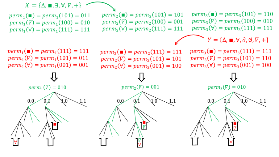
Note that the permutation permz𝑝𝑒𝑟subscript𝑚𝑧perm_{z} is a deterministic function of z𝑧z, i.e., at each band the same permutation is used to randomly permute the data points x𝑥x and y𝑦y. These permutations are chosen before mapping the data points. In Figure 3, we show how both x𝑥x and y𝑦y data points are first permuted randomly (using the same permutation) and then are mapped to the buckets in decision trees. Note that, here we call a pair positive, if they fall into the same bucket in at least one of the bands. Now, we show that these hashes are distribution sensitive.

Definition 3

The functions Φ:V:Φ𝑉\Phi:V\rightarrow\mathbb{R}, Ψ𝒜:V:superscriptΨ𝒜𝑉{\Psi}^{\mathcal{A}}:V\rightarrow\mathbb{R} and Ψ:V:superscriptΨ𝑉{\Psi}^{\mathcal{B}}:V\rightarrow\mathbb{R} are defined as follows. At root, Φ(root)=1Φ𝑟𝑜𝑜𝑡1\Phi({root})=1, Ψ𝒜(root)=1superscriptΨ𝒜𝑟𝑜𝑜𝑡1{\Psi}^{\mathcal{A}}({root})=1 and Ψ(root)=1superscriptΨ𝑟𝑜𝑜𝑡1{\Psi}^{\mathcal{B}}({root})=1, and for ai𝒜subscript𝑎𝑖𝒜a_{i}\in\mathcal{A}, bjsubscript𝑏𝑗b_{j}\in\mathcal{B} and vV𝑣𝑉v\in V, Φ(v)Φ𝑣\Phi(v), Ψ𝒜(v)superscriptΨ𝒜𝑣{\Psi}^{\mathcal{A}}(v), and Ψ(v)superscriptΨ𝑣{\Psi}^{\mathcal{B}}(v) are defined recursively as

Φ(f(v,ai,bj))Φ𝑓𝑣subscript𝑎𝑖subscript𝑏𝑗\displaystyle\Phi(f(v,a_{i},b_{j})) =\displaystyle= Φ(v)pij,vV,Φ𝑣subscript𝑝𝑖𝑗for-all𝑣𝑉\displaystyle\Phi(v)p_{ij},\forall v\in V, (21)
Ψ𝒜(f(v,ai,bj))superscriptΨ𝒜𝑓𝑣subscript𝑎𝑖subscript𝑏𝑗\displaystyle{\Psi}^{\mathcal{A}}(f(v,a_{i},b_{j})) =\displaystyle= Ψ𝒜(v)pi𝒜,vV,superscriptΨ𝒜𝑣superscriptsubscript𝑝𝑖𝒜for-all𝑣𝑉\displaystyle{\Psi}^{\mathcal{A}}(v)p_{i}^{\mathcal{A}},\forall v\in V, (22)
Ψ(f(v,ai,bj))superscriptΨ𝑓𝑣subscript𝑎𝑖subscript𝑏𝑗\displaystyle{\Psi}^{\mathcal{B}}(f(v,a_{i},b_{j})) =\displaystyle= Ψ(v)pj,vV.superscriptΨ𝑣superscriptsubscript𝑝𝑗for-all𝑣𝑉\displaystyle{\Psi}^{\mathcal{B}}(v)p_{j}^{\mathcal{B}},\forall v\in V. (23)

Moreover, Ψ:V:Ψ𝑉\Psi:V\rightarrow\mathbb{R} is defined as

Ψ(v)Ψ𝑣\displaystyle\Psi(v) =\displaystyle= Ψ𝒜(v)Ψ(v),vV.superscriptΨ𝒜𝑣superscriptΨ𝑣for-all𝑣𝑉\displaystyle{\Psi}^{\mathcal{A}}(v){\Psi}^{\mathcal{B}}(v),\forall v\in V. (24)

Refer to caption

Figure 3: With only a single band, many of the true pairs are missed (not called positives). Refer to (50) and (51) in order to see how multiple bands improve true positive rate. While the decision tree are not affected in any band 1z#bands1𝑧#𝑏𝑎𝑛𝑑𝑠1\leq z\leq\#bands, classes and queries are permuted by permz𝑝𝑒𝑟subscript𝑚𝑧perm_{z} (using the same permutation permz𝑝𝑒𝑟subscript𝑚𝑧perm_{z}) and then mapped to the buckets in decision trees. In this figure, all classes and queries are permuted through three permutations perm1(abc)=bac𝑝𝑒𝑟subscript𝑚1𝑎𝑏𝑐𝑏𝑎𝑐perm_{1}(abc)=bac, perm2(abc)=cba𝑝𝑒𝑟subscript𝑚2𝑎𝑏𝑐𝑐𝑏𝑎perm_{2}(abc)=cba and perm3(abc)=cab𝑝𝑒𝑟subscript𝑚3𝑎𝑏𝑐𝑐𝑎𝑏perm_{3}(abc)=cab. We showed how three of classes, i.e., ,,for-all{\color[rgb]{0,1,0}\blacksquare,\triangledown,\forall} and three of queries ,,for-all{\color[rgb]{1,0,0}\blacksquare,\triangledown,\forall} are permuted. How {\color[rgb]{0,1,0}\triangledown} is mapped through these three trees is shown similar to Figure 1. In the end, all the classes and queries designated to the buckets are shown. Note that, a pair is called positive if they intersect in at least one of the bands.
Lemma 1

The following properties hold:

Φ(v)Φ𝑣\displaystyle\Phi(v) =\displaystyle= Prob(vHz𝒜(x)Hz(y)(x,y)),𝑃𝑟𝑜𝑏𝑣superscriptsubscript𝐻𝑧𝒜𝑥conditionalsuperscriptsubscript𝐻𝑧𝑦𝑥𝑦similar-to\displaystyle Prob(v\in H_{z}^{\mathcal{A}}(x)\cap H_{z}^{\mathcal{B}}(y)\mid(x,y)\sim\mathbb{P}), (25)
Ψ(v)Ψ𝑣\displaystyle\Psi(v) =\displaystyle= Prob(vHz𝒜(x)Hz(y)(x,y)),𝑃𝑟𝑜𝑏𝑣superscriptsubscript𝐻𝑧𝒜𝑥conditionalsuperscriptsubscript𝐻𝑧𝑦𝑥𝑦similar-to\displaystyle Prob(v\in H_{z}^{\mathcal{A}}(x)\cap H_{z}^{\mathcal{B}}(y)\mid(x,y)\sim\mathbb{Q}), (26)
Ψ𝒜(v)superscriptΨ𝒜𝑣\displaystyle{\Psi}^{\mathcal{A}}(v) =\displaystyle= Prob(vHz𝒜(x)x𝒜),𝑃𝑟𝑜𝑏𝑣conditionalsuperscriptsubscript𝐻𝑧𝒜𝑥𝑥similar-tosuperscript𝒜\displaystyle Prob(v\in H_{z}^{\mathcal{A}}(x)\mid x\sim\mathbb{P}^{\mathcal{A}}), (27)
Ψ(v)superscriptΨ𝑣\displaystyle{\Psi}^{\mathcal{B}}(v) =\displaystyle= Prob(vHz(y)y).𝑃𝑟𝑜𝑏𝑣conditionalsuperscriptsubscript𝐻𝑧𝑦𝑦similar-tosuperscript\displaystyle Prob(v\in H_{z}^{\mathcal{B}}(y)\mid y\sim\mathbb{P}^{\mathcal{B}}). (28)
Remark 4

Note that the left side of ((25)(28))italic-(25italic-)italic-(28italic-)(\eqref{fam1}-\eqref{fam2}) is independent of z𝑧z while it seems like the right side depend on band z𝑧z. The proof of Lemma 1 in Appendix A shows that in fact it is independent of band z𝑧z.

Lemma 2

For any decision tree G𝐺G, satisfying the condition that for any pair of buckets v1,v2VBucketssubscript𝑣1subscript𝑣2subscript𝑉𝐵𝑢𝑐𝑘𝑒𝑡𝑠v_{1},v_{2}\in V_{Buckets}, v1subscript𝑣1v_{1} is not an ancestor or descendant of v2subscript𝑣2v_{2}, Hz𝒜(x)superscriptsubscript𝐻𝑧𝒜𝑥H_{z}^{\mathcal{A}}(x) and Hz(y)superscriptsubscript𝐻𝑧𝑦H_{z}^{\mathcal{B}}(y) defined in (19) and (20) are (,α(G),β(G),γ𝒜(G),γ(G))𝛼𝐺𝛽𝐺superscript𝛾𝒜𝐺superscript𝛾𝐺(\mathbb{P},\alpha(G),\beta(G),\gamma^{\mathcal{A}}(G),\gamma^{\mathcal{B}}(G))-sensitive where

α(G)𝛼𝐺\displaystyle\alpha(G) =\displaystyle= vVBuckets(G)Φ(v),subscript𝑣subscript𝑉𝐵𝑢𝑐𝑘𝑒𝑡𝑠𝐺Φ𝑣\displaystyle\sum_{v\in V_{Buckets}(G)}\Phi(v), (29)
β(G)𝛽𝐺\displaystyle\beta(G) =\displaystyle= vVBuckets(G)Ψ(v),subscript𝑣subscript𝑉𝐵𝑢𝑐𝑘𝑒𝑡𝑠𝐺Ψ𝑣\displaystyle\sum_{v\in V_{Buckets}(G)}\Psi(v), (30)
γ𝒜(G)superscript𝛾𝒜𝐺\displaystyle\gamma^{\mathcal{A}}(G) =\displaystyle= vVBuckets(G)Ψ𝒜(v),subscript𝑣subscript𝑉𝐵𝑢𝑐𝑘𝑒𝑡𝑠𝐺superscriptΨ𝒜𝑣\displaystyle\sum_{v\in V_{Buckets}(G)}{\Psi}^{\mathcal{A}}(v), (31)
γ(G)superscript𝛾𝐺\displaystyle\gamma^{\mathcal{B}}(G) =\displaystyle= vVBuckets(G)Ψ(v).subscript𝑣subscript𝑉𝐵𝑢𝑐𝑘𝑒𝑡𝑠𝐺superscriptΨ𝑣\displaystyle\sum_{v\in V_{Buckets}(G)}{\Psi}^{\mathcal{B}}(v). (32)

Proofs of Lemmas 1 and 2 are relegated to Appendix A. So far, we showed how to design ForestDSH using a decision tree structure. However, it is not yet clear how to map data points to these buckets. In the next section, we investigate this and provide an algorithm to design optimal decision trees.

4.1 Mapping Data Points

In the previous sections, we presented Algorithm 2 for solving (1) where we need to compute Hz𝒜(x)superscriptsubscript𝐻𝑧𝒜𝑥H_{z}^{\mathcal{A}}(x) and Hz(y)superscriptsubscript𝐻𝑧𝑦H_{z}^{\mathcal{B}}(y) by mapping data points to the buckets. We did not clarify how this mapping can be done efficiently. We present Algorithm 3 for mapping data points to the buckets using hash-table search, see Figure 2.

Algorithm 3 Mapping data points to the buckets using hash-table search
    Inputs: List of buckets VBucketssubscript𝑉𝐵𝑢𝑐𝑘𝑒𝑡𝑠V_{Buckets}, permutations permz,1z#bands𝑝𝑒𝑟subscript𝑚𝑧1𝑧#𝑏𝑎𝑛𝑑𝑠perm_{z},1\leq z\leq\#bands, and a set of data points X={x1,,xN}𝑋superscript𝑥1superscript𝑥𝑁X=\{x^{1},\cdots,x^{N}\}.
    Outputs: Hz𝒜(x)superscriptsubscript𝐻𝑧𝒜𝑥H_{z}^{\mathcal{A}}(x) for each xX𝑥𝑋x\in X and each band 1z#bands1𝑧#𝑏𝑎𝑛𝑑𝑠1\leq z\leq\#bands.
    Create an empty hash-table.
    Initialize Hz𝒜(x)=superscriptsubscript𝐻𝑧𝒜𝑥H_{z}^{\mathcal{A}}(x)=\varnothing for all xX𝑥𝑋x\in X and 1z#bands1𝑧#𝑏𝑎𝑛𝑑𝑠1\leq z\leq\#bands.
    For vVBuckets𝑣subscript𝑉𝐵𝑢𝑐𝑘𝑒𝑡𝑠v\in V_{Buckets}
         Insert Seq𝒜(v)𝑆𝑒superscript𝑞𝒜𝑣Seq^{\mathcal{A}}(v) into the hash-table.
    For z=1𝑧1z=1 to #bands#𝑏𝑎𝑛𝑑𝑠\#bands
         For xX𝑥𝑋x\in{X}
             Search permz(x)𝑝𝑒𝑟subscript𝑚𝑧𝑥perm_{z}(x) in the hash-table to find all vVBuckets𝑣subscript𝑉𝐵𝑢𝑐𝑘𝑒𝑡𝑠v\in V_{Buckets} for which Seq𝒜(v)𝑆𝑒superscript𝑞𝒜𝑣Seq^{\mathcal{A}}(v) is a prefix of permz(x)𝑝𝑒𝑟subscript𝑚𝑧𝑥perm_{z}(x), and insert v𝑣v into Hz𝒜(x)superscriptsubscript𝐻𝑧𝒜𝑥H_{z}^{\mathcal{A}}(x) (see Figure 3).
Remark 5

Queries are mapped to buckets using hash-table search similar to data points through Algorithm 3.

Note that we slightly modify the hash-table to search for values that are prefix of a query, rather than being exactly identical. In Section 5, we show that the complexity of Algorithms 2 and 3 can be formulated as:

ctree|V(G)|subscript𝑐𝑡𝑟𝑒𝑒𝑉𝐺\displaystyle c_{tree}|V(G)|
+(chashNα(G)+chashMα(G)+cinsertionNγ𝒜(G)α(G)+cinsertionMγ(G)α(G)+cposMNβ(G)α(G))log11TP,subscript𝑐𝑎𝑠𝑁𝛼𝐺subscript𝑐𝑎𝑠𝑀𝛼𝐺subscript𝑐𝑖𝑛𝑠𝑒𝑟𝑡𝑖𝑜𝑛𝑁superscript𝛾𝒜𝐺𝛼𝐺subscript𝑐𝑖𝑛𝑠𝑒𝑟𝑡𝑖𝑜𝑛𝑀superscript𝛾𝐺𝛼𝐺subscript𝑐𝑝𝑜𝑠𝑀𝑁𝛽𝐺𝛼𝐺11𝑇𝑃\displaystyle+\left(\frac{c_{hash}N}{\alpha(G)}+\frac{c_{hash}M}{\alpha(G)}+\frac{c_{insertion}N\gamma^{\mathcal{A}}(G)}{\alpha(G)}+\frac{c_{insertion}M\gamma^{\mathcal{B}}(G)}{\alpha(G)}+\frac{c_{pos}MN\beta(G)}{\alpha(G)}\right){\log\frac{1}{1-TP}}, (33)

where ctreesubscript𝑐𝑡𝑟𝑒𝑒c_{tree}, chashsubscript𝑐𝑎𝑠c_{hash}, cinsertionsubscript𝑐𝑖𝑛𝑠𝑒𝑟𝑡𝑖𝑜𝑛c_{insertion} and cpossubscript𝑐𝑝𝑜𝑠c_{pos} are constants not depending on N𝑁N. For the intuition behind (33), note that the first term ctree|V(G)|subscript𝑐𝑡𝑟𝑒𝑒𝑉𝐺c_{tree}|V(G)| stands for the time required for calculating and storing the tree. The second and third terms, i.e., (chashNα(G)+chashMα(G))log11TPsubscript𝑐𝑎𝑠𝑁𝛼𝐺subscript𝑐𝑎𝑠𝑀𝛼𝐺11𝑇𝑃\left(\frac{c_{hash}N}{\alpha(G)}+\frac{c_{hash}M}{\alpha(G)}\right){\log\frac{1}{1-TP}} denote the time needed for inserting data points to the hash-table. The fourth and fifth terms, i.e., (cinsertionNγ𝒜(G)α(G)+cinsertionMγ(G)α(G))log11TPsubscript𝑐𝑖𝑛𝑠𝑒𝑟𝑡𝑖𝑜𝑛𝑁superscript𝛾𝒜𝐺𝛼𝐺subscript𝑐𝑖𝑛𝑠𝑒𝑟𝑡𝑖𝑜𝑛𝑀superscript𝛾𝐺𝛼𝐺11𝑇𝑃\left(\frac{c_{insertion}N\gamma^{\mathcal{A}}(G)}{\alpha(G)}+\frac{c_{insertion}M\gamma^{\mathcal{B}}(G)}{\alpha(G)}\right){\log\frac{1}{1-TP}} stand for the time required for mapping the data points from the hash-table to buckets. Finally, the last term, i.e., (cposMNβ(G)α(G))log11TPsubscript𝑐𝑝𝑜𝑠𝑀𝑁𝛽𝐺𝛼𝐺11𝑇𝑃\left(\frac{c_{pos}MN\beta(G)}{\alpha(G)}\right){\log\frac{1}{1-TP}} is the time of brute-force checking within each bucket.

In order to bound (33) with O(Nλ)𝑂superscript𝑁𝜆O(N^{\lambda}) for some λ+𝜆superscript\lambda\in\mathbb{R}^{+}, it is necessary and sufficient to find a tree G𝐺G that satisfies the following constraints:

|V(G)|𝑉𝐺\displaystyle|V(G)| =\displaystyle= O(Nλ),𝑂superscript𝑁𝜆\displaystyle O(N^{\lambda}), (34)
α(G)β(G)𝛼𝐺𝛽𝐺\displaystyle\frac{\alpha(G)}{\beta(G)} =\displaystyle= Ω(N1+δλ),Ωsuperscript𝑁1𝛿𝜆\displaystyle\Omega(N^{1+\delta-\lambda}), (35)
α(G)γ𝒜(G)𝛼𝐺superscript𝛾𝒜𝐺\displaystyle\frac{\alpha(G)}{\gamma^{\mathcal{A}}(G)} =\displaystyle= Ω(N1λ),Ωsuperscript𝑁1𝜆\displaystyle\Omega(N^{1-\lambda}), (36)
α(G)γ(G)𝛼𝐺superscript𝛾𝐺\displaystyle\frac{\alpha(G)}{\gamma^{\mathcal{B}}(G)} =\displaystyle= Ω(Nδλ),Ωsuperscript𝑁𝛿𝜆\displaystyle\Omega(N^{\delta-\lambda}), (37)
α(G)𝛼𝐺\displaystyle{\alpha(G)} =\displaystyle= Ω(Nmax(1,δ)λ),Ωsuperscript𝑁1𝛿𝜆\displaystyle\Omega(N^{\max(1,\delta)-\lambda}), (38)

where δ=logMlogN𝛿𝑀𝑁{\delta}=\frac{\log M}{\log N}.

Theorem 1

Complexity of Algorithms 2 and 3 is equal to (33). Moreover, there exists a decision tree G𝐺G that is optimal and satisfies ((34)(38))italic-(34italic-)italic-(38italic-)(\eqref{order1}-\eqref{order3}) for λ𝜆\lambda defined in Definition 444.

Theorem 1 is proved in three steps: (a)𝑎(a). In Section 5, we prove that the complexity is equal to (33). (b)𝑏(b). Theorem 2 shows that the tree G𝐺G constructed by Algorithm 4 and presented in Section 6 satisfies ((34)-(38)) for λ𝜆\lambda defined in Definition 4. (c)𝑐(c). Theorem 3 shows that this is optimal.

5 Complexity Analysis

In this section, we bound the complexity of Algorithms 2 and 3 by (33). Note that, the complexity of Algorithms 2 and 3 is the summation of the following terms.

  1. 1.

    Tree construction complexity. ctree|V(G)|subscript𝑐𝑡𝑟𝑒𝑒𝑉𝐺c_{tree}|V(G)| is the tree construction complexity where ctreesubscript𝑐𝑡𝑟𝑒𝑒c_{tree} is a constant representing per node complexity of constructing a node and |V(G)|𝑉𝐺|V(G)| is the number of nodes in the tree.

  2. 2.

    Data mapping complexity. The complexity of this hash-table search grows with

    chash(#bands)|X|+cinsertionz=1#bandsxX|Hz𝒜(x)|subscript𝑐𝑎𝑠#𝑏𝑎𝑛𝑑𝑠𝑋subscript𝑐𝑖𝑛𝑠𝑒𝑟𝑡𝑖𝑜𝑛superscriptsubscript𝑧1#𝑏𝑎𝑛𝑑𝑠subscript𝑥𝑋superscriptsubscript𝐻𝑧𝒜𝑥\displaystyle c_{hash}(\#bands)|{X}|+c_{insertion}\sum_{z=1}^{\#bands}\sum_{x\in X}|H_{z}^{\mathcal{A}}(x)| (39)
    +chash(#bands)|Y|+cinsertionz=1#bandsyY|Hz(y)|,subscript𝑐𝑎𝑠#𝑏𝑎𝑛𝑑𝑠𝑌subscript𝑐𝑖𝑛𝑠𝑒𝑟𝑡𝑖𝑜𝑛superscriptsubscript𝑧1#𝑏𝑎𝑛𝑑𝑠subscript𝑦𝑌superscriptsubscript𝐻𝑧𝑦\displaystyle+c_{hash}(\#bands)|{Y}|+c_{insertion}\sum_{z=1}^{\#bands}\sum_{y\in Y}|H_{z}^{\mathcal{B}}(y)|, (40)

    where chashsubscript𝑐𝑎𝑠c_{hash} and cinsertionsubscript𝑐𝑖𝑛𝑠𝑒𝑟𝑡𝑖𝑜𝑛c_{insertion} represent complexity of insertion in the hash-table and insertion in the buckets, respectively.

  3. 3.

    Complexity of checking positive calls. (#bands)cposxX,yY|Hz𝒜(x)Hz(y)|)(\#bands)c_{pos}\sum_{x\in X,y\in Y}|H_{z}^{\mathcal{A}}(x)\cap H_{z}^{\mathcal{B}}(y)|\big{)} is the complexity of checking positive calls where cpossubscript𝑐𝑝𝑜𝑠c_{pos} is a constant representing the complexity of computing (yx)conditional𝑦𝑥\mathbb{P}(y\mid x) for a positive. Note that, ctreesubscript𝑐𝑡𝑟𝑒𝑒c_{tree}, chashsubscript𝑐𝑎𝑠c_{hash}, cinsertionsubscript𝑐𝑖𝑛𝑠𝑒𝑟𝑡𝑖𝑜𝑛c_{insertion} and cpossubscript𝑐𝑝𝑜𝑠c_{pos} are constants not depending on N𝑁N. From ((11)(15))italic-(11italic-)italic-(15italic-)(\eqref{family1}-\eqref{family5}), we have

    𝔼(z=1#bandsxX|Hz𝒜(x)|)𝔼superscriptsubscript𝑧1#𝑏𝑎𝑛𝑑𝑠subscript𝑥𝑋superscriptsubscript𝐻𝑧𝒜𝑥\displaystyle\mathbb{E}\big{(}\sum_{z=1}^{\#bands}\sum_{x\in X}|H_{z}^{\mathcal{A}}(x)|\big{)} (41)
    =\displaystyle= 𝔼(z=1#bandsxX,vVBuckets(G)1xv)𝔼superscriptsubscript𝑧1#𝑏𝑎𝑛𝑑𝑠subscriptformulae-sequence𝑥𝑋𝑣subscript𝑉𝐵𝑢𝑐𝑘𝑒𝑡𝑠𝐺subscript1𝑥𝑣\displaystyle{{}\mathbb{E}\big{(}\sum_{z=1}^{\#bands}\sum_{x\in X,v\in V_{Buckets}(G)}1_{x\in v}\big{)}}
    =\displaystyle= (#bands)NvVBuckets(G)Ψ𝒜(v)=(#bands)Nγ𝒜(G)#𝑏𝑎𝑛𝑑𝑠𝑁subscript𝑣subscript𝑉𝐵𝑢𝑐𝑘𝑒𝑡𝑠𝐺superscriptΨ𝒜𝑣#𝑏𝑎𝑛𝑑𝑠𝑁superscript𝛾𝒜𝐺\displaystyle(\#bands)N\sum_{v\in V_{Buckets}(G)}{\Psi}^{\mathcal{A}}(v)=(\#bands)N\gamma^{\mathcal{A}}(G)
    𝔼(z=1#bandsyY|Hz(y)|)𝔼superscriptsubscript𝑧1#𝑏𝑎𝑛𝑑𝑠subscript𝑦𝑌superscriptsubscript𝐻𝑧𝑦\displaystyle\mathbb{E}\big{(}\sum_{z=1}^{\#bands}\sum_{y\in Y}|H_{z}^{\mathcal{B}}(y)|\big{)}
    =\displaystyle= 𝔼(z=1#bandsyY,vVBuckets(G)1yv)𝔼superscriptsubscript𝑧1#𝑏𝑎𝑛𝑑𝑠subscriptformulae-sequence𝑦𝑌𝑣subscript𝑉𝐵𝑢𝑐𝑘𝑒𝑡𝑠𝐺subscript1𝑦𝑣\displaystyle\mathbb{E}\big{(}\sum_{z=1}^{\#bands}\sum_{y\in Y,v\in V_{Buckets}(G)}1_{y\in v}\big{)} (43)
    =\displaystyle= (#bands)MvVBuckets(G)Ψ(v)=(#bands)Mγ(G).#𝑏𝑎𝑛𝑑𝑠𝑀subscript𝑣subscript𝑉𝐵𝑢𝑐𝑘𝑒𝑡𝑠𝐺superscriptΨ𝑣#𝑏𝑎𝑛𝑑𝑠𝑀superscript𝛾𝐺\displaystyle(\#bands)M\sum_{v\in V_{Buckets}(G)}{\Psi}^{\mathcal{B}}(v)=(\#bands)M\gamma^{\mathcal{B}}(G). (44)

    Note that, the total number of collision for random pairs is the sum of number of buckets that they intersect at. Therefore, we conclude that

    𝔼(z=1#bandsxX,yY|Hz𝒜(x)Hz(y)|)𝔼superscriptsubscript𝑧1#𝑏𝑎𝑛𝑑𝑠subscriptformulae-sequence𝑥𝑋𝑦𝑌superscriptsubscript𝐻𝑧𝒜𝑥superscriptsubscript𝐻𝑧𝑦\displaystyle\mathbb{E}\big{(}\sum_{z=1}^{\#bands}\sum_{x\in X,y\in Y}|H_{z}^{\mathcal{A}}(x)\cap H_{z}^{\mathcal{B}}(y)|\big{)} (45)
    =\displaystyle= z=1#bandsxX,yYProb(|Hz𝒜(x)Hz(y)|=1)superscriptsubscript𝑧1#𝑏𝑎𝑛𝑑𝑠subscriptformulae-sequence𝑥𝑋𝑦𝑌𝑃𝑟𝑜𝑏superscriptsubscript𝐻𝑧𝒜𝑥superscriptsubscript𝐻𝑧𝑦1\displaystyle\sum_{z=1}^{\#bands}\sum_{x\in X,y\in Y}Prob\big{(}|H_{z}^{\mathcal{A}}(x)\cap H_{z}^{\mathcal{B}}(y)|=1\big{)}
    =\displaystyle= z=1#bandsxX,yYvVBuckets(G)Prob(vHz𝒜(x),vHz(y))superscriptsubscript𝑧1#𝑏𝑎𝑛𝑑𝑠subscriptformulae-sequence𝑥𝑋𝑦𝑌subscript𝑣subscript𝑉𝐵𝑢𝑐𝑘𝑒𝑡𝑠𝐺𝑃𝑟𝑜𝑏formulae-sequence𝑣superscriptsubscript𝐻𝑧𝒜𝑥𝑣superscriptsubscript𝐻𝑧𝑦\displaystyle\sum_{z=1}^{\#bands}{\color[rgb]{0,0,0}\sum_{x\in X,y\in Y}\sum_{v\in V_{Buckets}(G)}}Prob\big{(}v\in H_{z}^{\mathcal{A}}(x),v\in H_{z}^{\mathcal{B}}(y)\big{)} (46)
    =\displaystyle= (#bands)MNvVBuckets(G)Ψ(v)=(#bands)MNβ(G),#𝑏𝑎𝑛𝑑𝑠𝑀𝑁subscript𝑣subscript𝑉𝐵𝑢𝑐𝑘𝑒𝑡𝑠𝐺Ψ𝑣#𝑏𝑎𝑛𝑑𝑠𝑀𝑁𝛽𝐺\displaystyle(\#bands)MN\sum_{v\in V_{Buckets}(G)}\Psi(v)=(\#bands)MN\beta(G), (47)

    where (45) is concluded as H𝒜(x)H(y)1delimited-∣∣superscript𝐻𝒜𝑥superscript𝐻𝑦1{\mid H^{\mathcal{A}}(x)\cap H^{\mathcal{B}}(y)\mid}\leq 1.

Now, the question is how we can select #bands#𝑏𝑎𝑛𝑑𝑠\#bands such that the true positive rate, defined as the ratio of true pairs that are called positive is high. In each band, the chance of a pair (x,y)similar-to𝑥𝑦(x,y)\sim\mathbb{P} being called positive is computed as α(G)=vVBuckets(G)Φ(v)𝛼𝐺subscript𝑣subscript𝑉𝐵𝑢𝑐𝑘𝑒𝑡𝑠𝐺Φ𝑣\alpha(G)=\sum_{v\in V_{Buckets}(G)}\Phi(v). Therefore, the overall true positive rate can be computed as:

TP𝑇𝑃\displaystyle TP =\displaystyle= Prob((x,y) called positive in Algorithm 2 (x,y))𝑃𝑟𝑜𝑏similar-toconditional𝑥𝑦 called positive in Algorithm 2 𝑥𝑦\displaystyle Prob((x,y)\mbox{~{}called positive in Algorithm \ref{algorithm_Max}~{}}\mid(x,y)\sim\mathbb{P}) (48)
=\displaystyle= 1z=1#bands(1vVBucketsProb(vHz𝒜(x)Hz(y)(x,y)))1superscriptsubscriptproduct𝑧1#𝑏𝑎𝑛𝑑𝑠1subscript𝑣subscript𝑉𝐵𝑢𝑐𝑘𝑒𝑡𝑠𝑃𝑟𝑜𝑏𝑣superscriptsubscript𝐻𝑧𝒜𝑥conditionalsuperscriptsubscript𝐻𝑧𝑦𝑥𝑦similar-to\displaystyle 1-\prod_{z=1}^{\#bands}\left(1-\sum_{v\in V_{Buckets}}Prob(v\in H_{z}^{\mathcal{A}}(x)\cap H_{z}^{\mathcal{B}}(y)\mid(x,y)\sim\mathbb{P})\right) (49)
=\displaystyle= 1(1α(G))#bands.1superscript1𝛼𝐺#𝑏𝑎𝑛𝑑𝑠\displaystyle 1-{(1-\alpha(G))}^{\#bands}. (50)

Using (50), and the inequality (1x)cx<ecsuperscript1𝑥𝑐𝑥superscript𝑒𝑐(1-x)^{\frac{c}{x}}<e^{-c}, the minimum possible value of #bands#𝑏𝑎𝑛𝑑𝑠\#bands to ensure true positive rate TP𝑇𝑃TP can be computed as

#bands#𝑏𝑎𝑛𝑑𝑠\displaystyle\#bands =\displaystyle= log11TPα(G),11𝑇𝑃𝛼𝐺\displaystyle\lceil\frac{\log\frac{1}{1-TP}}{\alpha(G)}\rceil, (51)

where r𝑟\lceil r\rceil stands for the smallest integer greater than or equal to r𝑟r. Therefore, the total complexity is equal to (33).

6 Constructing optimal decision trees for ForestDSH

In this section, we present an algorithm to design decision trees with complexity O(Nλ)𝑂superscript𝑁superscript𝜆O(N^{\lambda^{*}}), where λsuperscript𝜆\lambda^{*} is defined below, and we show that it is the optimal decision tree.

Definition 4

Given probability distributions P=[pij]𝑃delimited-[]subscript𝑝𝑖𝑗P=[p_{ij}] and Q=[qij]𝑄delimited-[]subscript𝑞𝑖𝑗Q=[q_{ij}], 1ik,1jlformulae-sequence1𝑖𝑘1𝑗𝑙1\leq i\leq k,1\leq j\leq l, and number of queries and classes M𝑀M and N𝑁N define δ=logMlogN𝛿𝑀𝑁\delta=\frac{\log M}{\log N} and

\displaystyle\mathcal{I} =\displaystyle= {(μ,ν,η)3|min(μ,ν)η0,\displaystyle\{(\mu,\nu,\eta)\in\mathbb{R}^{3}|\min(\mu,\nu)\geq\eta\geq 0, (52)
1ik,1jlpij1+μ+νη(pi𝒜)μ(pj)ν=1},\displaystyle\sum_{1\leq i\leq k,1\leq j\leq l}p_{ij}^{1+\mu+\nu-\eta}{(p_{i}^{\mathcal{A}})}^{-\mu}{(p_{j}^{\mathcal{B}})}^{-\nu}=1\},
(μ,ν,η)superscript𝜇superscript𝜈superscript𝜂\displaystyle(\mu^{*},\nu^{*},\eta^{*}) =\displaystyle= Argmaxmax(1,δ)+μ+νδ1+μ+νη,𝐴𝑟𝑔subscript1𝛿𝜇𝜈𝛿1𝜇𝜈𝜂\displaystyle Arg\max_{\mathcal{I}}\frac{\max(1,\delta)+\mu+\nu\delta}{1+\mu+\nu-\eta}, (53)
rijsuperscriptsubscript𝑟𝑖𝑗\displaystyle r_{ij}^{*} =\displaystyle= pij1+μ+νη(pi𝒜)μ(pj)ν,superscriptsubscript𝑝𝑖𝑗1superscript𝜇superscript𝜈superscript𝜂superscriptsuperscriptsubscript𝑝𝑖𝒜superscript𝜇superscriptsuperscriptsubscript𝑝𝑗superscript𝜈\displaystyle{\color[rgb]{0,0,0}p_{ij}^{1+\mu^{*}+\nu^{*}-\eta^{*}}{(p_{i}^{\mathcal{A}})}^{-\mu^{*}}{(p_{j}^{\mathcal{B}})}^{-\nu^{*}}}, (54)
nsuperscript𝑛\displaystyle n^{*} =\displaystyle= (max(1,δ)λ)logNrijlogpijrij,1𝛿superscript𝜆𝑁superscriptsubscript𝑟𝑖𝑗subscript𝑝𝑖𝑗superscriptsubscript𝑟𝑖𝑗\displaystyle{\color[rgb]{0,0,0}\frac{(\max(1,\delta)-\lambda^{*})\log N}{\sum r_{ij}^{*}\log\frac{p_{ij}}{r_{ij}^{*}}}}, (55)
λsuperscript𝜆\displaystyle\lambda^{*} =\displaystyle= max(1,δ)+μ+νδ1+μ+νη.1𝛿superscript𝜇superscript𝜈𝛿1superscript𝜇superscript𝜈superscript𝜂\displaystyle\frac{\max(1,\delta)+\mu^{*}+\nu^{*}\delta}{1+\mu^{*}+\nu^{*}-\eta^{*}}. (56)
Remark 6

For any probability distribution \mathbb{P}, the parameters μsuperscript𝜇\mu^{*}, νsuperscript𝜈\nu^{*}, ηsuperscript𝜂\eta^{*} and λsuperscript𝜆\lambda^{*} can be derived numerically from Algorithm 5 in  Appendix  B. The intuition  behind  the  definition  of   \mathcal{I} and (μ,ν,η)superscript𝜇superscript𝜈superscript𝜂(\mu^{*},\nu^{*},\eta^{*}) is that in Lemma 4 in Section 6.1 we show that for any decision tree G𝐺G and the variables Φ(v)Φ𝑣\Phi(v), Ψ𝒜(v)superscriptΨ𝒜𝑣{\Psi}^{\mathcal{A}}(v), Ψ(v)superscriptΨ𝑣{\Psi}^{\mathcal{B}}(v) and Ψ(v)Ψ𝑣\Psi(v) defined in (21)-(24), we have
vVBuckets(G)(Φ(v))1+μ+νη(Ψ𝒜(v))μ+η(Ψ(v))ν+η(Ψ(v))η1subscript𝑣subscript𝑉𝐵𝑢𝑐𝑘𝑒𝑡𝑠𝐺superscriptΦ𝑣1𝜇𝜈𝜂superscriptsuperscriptΨ𝒜𝑣𝜇𝜂superscriptsuperscriptΨ𝑣𝜈𝜂superscriptΨ𝑣𝜂1\sum_{v\in V_{Buckets}(G)}{\big{(}\Phi(v)\big{)}}^{1+\mu+\nu-\eta}{\big{(}{\Psi}^{\mathcal{A}}(v)\big{)}}^{-\mu+\eta}{\big{(}{\Psi}^{\mathcal{B}}(v)\big{)}}^{-\nu+\eta}{\big{(}\Psi(v)\big{)}}^{-\eta}\leq 1 if (μ,ν,η)𝜇𝜈𝜂(\mu,\nu,\eta)\in\mathcal{I}. Moreover, in proof of Theorem 2 we show that (μ,ν,η)superscript𝜇superscript𝜈superscript𝜂(\mu^{*},\nu^{*},\eta^{*}) are Lagrangian multipliers in an optimization problem to minimize the search complexity in Algorithm 2 while retaining a nearly perfect recovery. Consider the optimal decision tree and all the nodes v𝑣v satisfying

  1. 1.

    Depth of the node v𝑣v is nsuperscript𝑛n^{*}.

  2. 2.

    For any 1ik,1jlformulae-sequence1𝑖𝑘1𝑗𝑙1\leq i\leq k,1\leq j\leq l, the ratio of times we have aisubscript𝑎𝑖a_{i} at s𝑠s-th position of x𝑥x and bjsubscript𝑏𝑗b_{j} at s𝑠s-th position of y𝑦y in all 1sn1𝑠superscript𝑛1\leq s\leq n^{*} is rijsubscript𝑟𝑖𝑗r_{ij}.

The node v𝑣v or one of its ancestors is designated as a bucket by Algorithm 4. This is proved in Section 6.2.

In Algorithm 4, we provide an approach for designing decision trees with complexity O(Nλ)𝑂superscript𝑁superscript𝜆O(N^{\lambda^{*}}). The algorithm starts with the root, and at each step, it either accepts a node as a bucket, prunes a node, or branches a node into kl𝑘𝑙kl children based on the following constraints555If for any node the constraints for accepting as a bucket and pruning hold simultaneously, the algorithm accepts the node as a bucket. :

{Φ(v)Ψ(v)C1N1+δλ:Accept bucket,Φ(v)Ψ𝒜(v)C2N1λ:Prune,Φ(v)Ψ(v)C3Nδλ:Prune,otherwise:Branch into the kl children.\displaystyle\left\{\begin{matrix}\frac{\Phi(v)}{\Psi(v)}\geq C_{1}{N^{1+\delta-\lambda^{*}}}&:\mbox{Accept bucket},~{}~{}~{}~{}~{}~{}~{}~{}~{}~{}~{}~{}~{}~{}~{}~{}\\ \frac{\Phi(v)}{{\Psi}^{\mathcal{A}}(v)}\leq C_{2}N^{1-\lambda^{*}}&:\mbox{{}Prune},~{}~{}~{}~{}~{}~{}~{}~{}~{}~{}~{}~{}~{}~{}~{}~{}~{}~{}~{}~{}~{}~{}~{}~{}~{}~{}~{}\\ \frac{\Phi(v)}{{\Psi}^{\mathcal{B}}(v)}\leq C_{3}N^{\delta-\lambda^{*}}&:\mbox{{}Prune,}~{}~{}~{}~{}~{}~{}~{}~{}~{}~{}~{}~{}~{}~{}~{}~{}~{}~{}~{}~{}~{}~{}~{}~{}~{}~{}~{}\\ otherwise&:\mbox{Branch into the $kl$ children.}\end{matrix}\right. (57)

Note that, for the cases where pij=0subscript𝑝𝑖𝑗0p_{ij}=0, we simply remove that branch, therefore, we assume all the pijsubscript𝑝𝑖𝑗p_{ij} are positive real numbers. In Section 5, we prove that in order to bound the complexity in (33) with O(Nλ)𝑂superscript𝑁𝜆O(N^{\lambda}) for some λ+𝜆superscript\lambda\in\mathbb{R}^{+}, it is necessary and sufficient to find a decision tree G𝐺G that satisfies the constraints ((34)(38))italic-(34italic-)italic-(38italic-)(\eqref{order1}-\eqref{order3}).

Remark 7

In Theorem 3, we prove that the decision tree construction of Algorithm 4 results in a tree with complexity O(Nλ)𝑂superscript𝑁superscript𝜆O(N^{\lambda^{*}}) by setting C1=C2=C3=p0q0subscript𝐶1subscript𝐶2subscript𝐶3subscript𝑝0subscript𝑞0C_{1}=C_{2}=C_{3}=p_{0}q_{0} where p0subscript𝑝0p_{0} and q0subscript𝑞0q_{0} are defined as i,jpijsubscriptproduct𝑖𝑗subscript𝑝𝑖𝑗\prod_{i,j}p_{ij} and min(i,jqij,i(pi𝒜)l,j(pj)k)subscriptproduct𝑖𝑗subscript𝑞𝑖𝑗subscriptproduct𝑖superscriptsuperscriptsubscript𝑝𝑖𝒜𝑙subscriptproduct𝑗superscriptsuperscriptsubscript𝑝𝑗𝑘\min(\prod_{i,j}q_{ij},\prod_{i}{(p_{i}^{\mathcal{A}})}^{l},\prod_{j}{(p_{j}^{\mathcal{B}})}^{k}). Pessimistic lower bounds C1=C2=C3=p0q0subscript𝐶1subscript𝐶2subscript𝐶3subscript𝑝0subscript𝑞0C_{1}=C_{2}=C_{3}=p_{0}q_{0} are derived in proof of Theorem 3 and in practice C1subscript𝐶1C_{1}, C2subscript𝐶2C_{2} and C3subscript𝐶3C_{3} are chosen in a way that the best complexity is achieved.

Example 1

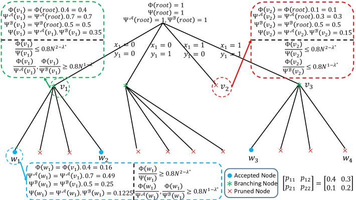
Here, we focus on the case where 𝒜={0,1},={0,1}formulae-sequence𝒜0101\mathcal{A}=\{0,1\},\mathcal{B}=\{0,1\}, P=[0.40.30.10.2]𝑃matrix0.40.30.10.2P=\begin{bmatrix}0.4&0.3\\ 0.1&0.2\end{bmatrix}, Q=[0.350.350.150.15]𝑄matrix0.350.350.150.15Q=\begin{bmatrix}0.35&0.35\\ 0.15&0.15\end{bmatrix}, δ=1𝛿1\delta=1, and M=N=4𝑀𝑁4M=N=4. From Algorithm 5, we have μ=12.0791superscript𝜇12.0791\mu^{*}=12.0791, ν=13.4206superscript𝜈13.4206\nu^{*}=13.4206, η=11.0959superscript𝜂11.0959\eta^{*}=11.0959, λ=1.7203superscript𝜆1.7203\lambda^{*}=1.7203. The decision tree is constructed from Algorithm 4 and is depicted in Figure 4. The nodes in the tree that are selected as bucket, i.e., satisfying Φ(v)Ψ(v)C1N1+δλΦ𝑣Ψ𝑣subscript𝐶1superscript𝑁1𝛿superscript𝜆\frac{\Phi(v)}{\Psi(v)}\geq C_{1}{N^{1+\delta-\lambda^{*}}}, are shown with a green check mark, and the nodes pruned out, satisfying either Φ(v)Ψ𝒜(v)C2N1λΦ𝑣superscriptΨ𝒜𝑣subscript𝐶2superscript𝑁1superscript𝜆\frac{\Phi(v)}{{\Psi}^{\mathcal{A}}(v)}\leq C_{2}N^{1-\lambda^{*}} or Φ(v)Ψ(v)C3NδλΦ𝑣superscriptΨ𝑣subscript𝐶3superscript𝑁𝛿superscript𝜆\frac{\Phi(v)}{{\Psi}^{\mathcal{B}}(v)}\leq C_{3}N^{\delta-\lambda^{*}} are shown with a red cross. For the non-leaf (intermediate) nodes, none of the above constraints holds. The bold edges show the paths in the tree corresponding to the data point x=(0,0)𝑥00x=(0,0). In this case, x𝑥x falls into a single bucket w1subscript𝑤1w_{1}.

Refer to caption

Figure 4: The decision tree and functions Φ(v)Φ𝑣\Phi(v), Ψ𝒜(v)superscriptΨ𝒜𝑣{\Psi}^{\mathcal{A}}(v), Ψ(v)superscriptΨ𝑣{\Psi}^{\mathcal{B}}(v) and Ψ(v)Ψ𝑣\Psi(v) are illustrated for 𝒜={0,1},={0,1}formulae-sequence𝒜0101\mathcal{A}=\{0,1\},\mathcal{B}=\{0,1\}, C1=C2=C3=0.8subscript𝐶1subscript𝐶2subscript𝐶30.8C_{1}=C_{2}=C_{3}=0.8 and N=5𝑁5N=5. For all of the nodes v1subscript𝑣1v_{1}, v2subscript𝑣2v_{2} and w1subscript𝑤1w_{1}, how the decisions are made are explained in the figure. For instance, consider the node w1subscript𝑤1w_{1}. For this node, Φ(w1)Φsubscript𝑤1\Phi(w_{1}), Ψ𝒜(w1)superscriptΨ𝒜subscript𝑤1{\Psi}^{\mathcal{A}}(w_{1}), Ψ(w1)superscriptΨsubscript𝑤1{\Psi}^{\mathcal{B}}(w_{1}) are derived from ((21)(23))italic-(21italic-)italic-(23italic-)(\eqref{def_a}-\eqref{def_a3}). On the other hand, from (57) this node is accepted as a bucket as Φ(w1)Ψ(w1)=1.310.8N2λ=1.26Φsubscript𝑤1Ψsubscript𝑤11.310.8superscript𝑁2superscript𝜆1.26\frac{\Phi(w_{1})}{\Psi(w_{1})}=1.31\geq 0.8N^{2-\lambda^{*}}=1.26. Note that, λ=1.72superscript𝜆1.72\lambda^{*}=1.72 from (56) and Algorithm 5.
Algorithm 4 Recursive construction of the decision tree
  Inputs: C1subscript𝐶1C_{1}, C2subscript𝐶2C_{2}, C3subscript𝐶3C_{3}, δ𝛿\delta, 𝒜𝒜\mathcal{A}, \mathcal{B}, P𝑃{P}, M𝑀M and N𝑁N. ##\# We use Algorithm 5 to derive μ,ν,η,λsuperscript𝜇superscript𝜈superscript𝜂superscript𝜆\mu^{*},\nu^{*},\eta^{*},\lambda^{*}, δ𝛿\delta.
  Outputs: G=(V,E,f)𝐺𝑉𝐸𝑓G=(V,E,f) and a subset of leaf nodes of the decision tree VBucketssubscript𝑉𝐵𝑢𝑐𝑘𝑒𝑡𝑠V_{Buckets}.
  Initialization:
      Seq𝒜(root)𝑆𝑒superscript𝑞𝒜𝑟𝑜𝑜𝑡Seq^{\mathcal{A}}{(root)}\leftarrow\varnothing, Seq(root)𝑆𝑒superscript𝑞𝑟𝑜𝑜𝑡Seq^{\mathcal{B}}{(root)}\leftarrow\varnothing.
      Φ(root)1Φ𝑟𝑜𝑜𝑡1\Phi(root)\leftarrow 1Ψ𝒜(root)1superscriptΨ𝒜𝑟𝑜𝑜𝑡1{\Psi}^{\mathcal{A}}(root)\leftarrow 1Ψ(root)1superscriptΨ𝑟𝑜𝑜𝑡1{\Psi}^{\mathcal{B}}(root)\leftarrow 1Ψ(root)1Ψ𝑟𝑜𝑜𝑡1\Psi(root)\leftarrow 1.
      Recursive TreeConstruction(root)𝑇𝑟𝑒𝑒𝐶𝑜𝑛𝑠𝑡𝑟𝑢𝑐𝑡𝑖𝑜𝑛𝑟𝑜𝑜𝑡TreeConstruction(root).
  Procedure TreeConstruction(v)𝑇𝑟𝑒𝑒𝐶𝑜𝑛𝑠𝑡𝑟𝑢𝑐𝑡𝑖𝑜𝑛𝑣TreeConstruction(v).
      For ai𝒜subscript𝑎𝑖𝒜a_{i}\in\mathcal{A}
          For bjsubscript𝑏𝑗b_{j}\in\mathcal{B}
              Create a new node w𝑤w.  ##\# The node is created only if pij0subscript𝑝𝑖𝑗0p_{ij}\neq 0.
              Φ(w)Φ(v)pijΦ𝑤Φ𝑣subscript𝑝𝑖𝑗\Phi(w)\leftarrow\Phi(v)p_{ij}
              Ψ𝒜(w)Ψ𝒜(v)pi𝒜superscriptΨ𝒜𝑤superscriptΨ𝒜𝑣superscriptsubscript𝑝𝑖𝒜{\Psi}^{\mathcal{A}}(w)\leftarrow{\Psi}^{\mathcal{A}}(v)p_{i}^{\mathcal{A}}
              Ψ(w)Ψ(v)pjsuperscriptΨ𝑤superscriptΨ𝑣superscriptsubscript𝑝𝑗{\Psi}^{\mathcal{B}}(w)\leftarrow{\Psi}^{\mathcal{B}}(v)p_{j}^{\mathcal{B}}
              Ψ(w)Ψ𝒜(w)Ψ(w)Ψ𝑤superscriptΨ𝒜𝑤superscriptΨ𝑤\Psi(w)\leftarrow{\Psi}^{\mathcal{A}}(w){\Psi}^{\mathcal{B}}(w)
              f(v,ai,bj)w𝑓𝑣subscript𝑎𝑖subscript𝑏𝑗𝑤f(v,a_{i},b_{j})\leftarrow w
              Seq𝒜(w)Seq𝒜(v)𝑆𝑒superscript𝑞𝒜𝑤𝑆𝑒superscript𝑞𝒜𝑣Seq^{\mathcal{A}}(w)\leftarrow Seq^{\mathcal{A}}(v), Seq(w)Seq(v)𝑆𝑒superscript𝑞𝑤𝑆𝑒superscript𝑞𝑣Seq^{\mathcal{B}}(w)\leftarrow Seq^{\mathcal{B}}(v)
              Seq𝒜(w).append(ai)formulae-sequence𝑆𝑒superscript𝑞𝒜𝑤𝑎𝑝𝑝𝑒𝑛𝑑subscript𝑎𝑖Seq^{\mathcal{A}}(w).append(a_{i}), Seq(w).append(bj)formulae-sequence𝑆𝑒superscript𝑞𝑤𝑎𝑝𝑝𝑒𝑛𝑑subscript𝑏𝑗Seq^{\mathcal{B}}(w).append(b_{j})
              If Φ(w)Ψ(w)C1N1+δλΦ𝑤Ψ𝑤subscript𝐶1superscript𝑁1𝛿superscript𝜆\frac{\Phi(w)}{\Psi(w)}\geq C_{1}{N^{1+\delta-\lambda^{*}}}                                                         ##\#Accept bucket
                  VBuckets.insert(w)formulae-sequencesubscript𝑉𝐵𝑢𝑐𝑘𝑒𝑡𝑠𝑖𝑛𝑠𝑒𝑟𝑡𝑤V_{Buckets}.insert(w)
              Else If Φ(w)Ψ𝒜(w)C2N1λΦ𝑤superscriptΨ𝒜𝑤subscript𝐶2superscript𝑁1superscript𝜆\frac{\Phi(w)}{{\Psi}^{\mathcal{A}}(w)}\geq C_{2}N^{1-\lambda^{*}} and Φ(w)Ψ(w)C3NδλΦ𝑤superscriptΨ𝑤subscript𝐶3superscript𝑁𝛿superscript𝜆\frac{\Phi(w)}{{\Psi}^{\mathcal{B}}(w)}\geq C_{3}N^{\delta-\lambda^{*}}                   ##\#Branch
                  TreeConstruction(w)𝑇𝑟𝑒𝑒𝐶𝑜𝑛𝑠𝑡𝑟𝑢𝑐𝑡𝑖𝑜𝑛𝑤TreeConstruction(w)
              Else                                                                                ##\#Prune
                  f(v,ai,bj)null𝑓𝑣subscript𝑎𝑖subscript𝑏𝑗𝑛𝑢𝑙𝑙f(v,a_{i},b_{j})\leftarrow null.
Theorem 2

No decision tree exists with overall complexity below O(Nλ)𝑂superscript𝑁superscript𝜆O(N^{\lambda^{*}}).

Theorem 3

The decision tree construction of Algorithm 4 described in Remark 7 results in a tree with complexity O(Nλ)𝑂superscript𝑁superscript𝜆O(N^{\lambda^{*}}).

In other words, Theorem 3 proves that the tree G𝐺G constructed by Algorithm 4 satisfies ((34)-(38)), and Theorem 2 shows that this is the optimal decision tree. For proofs of Theorems 2 and 3, see Sections 6.1 and 6.2. Note that, not only Theorem 3 guarantees that the number of the nodes in our decision tree is bounded by O(Nλ)𝑂superscript𝑁superscript𝜆O(N^{\lambda^{*}}) but also it guarantees that the run time for mapping the data points to the decision tree and the number of comparisons that we need to do for the nodes with the collision is bounded by O(Nλ)𝑂superscript𝑁superscript𝜆O(N^{\lambda^{*}}), see complexity equation (33) in Section 4.1.

Theorem 4 (Noise Robustness)

Assume that the decision tree of Algorithm 4 described in (57) is constructed based on distribution P=[pij]𝑃delimited-[]subscript𝑝𝑖𝑗P=[p_{ij}] while the data is generated from unknown P=[pij]superscript𝑃delimited-[]subscriptsuperscript𝑝𝑖𝑗P^{\prime}=[p^{\prime}_{ij}] satisfying pij1+ϵpijpij(1+ϵ)subscript𝑝𝑖𝑗1italic-ϵsubscriptsuperscript𝑝𝑖𝑗subscript𝑝𝑖𝑗1italic-ϵ\frac{p_{ij}}{1+\epsilon}\leq p^{\prime}_{ij}\leq{p_{ij}}{(1+\epsilon)} for all 1ik,1jlformulae-sequence1𝑖𝑘1𝑗𝑙1\leq i\leq k,1\leq j\leq l and some ϵ>0italic-ϵ0\epsilon>0. Then, it is possible to design an algorithm with complexity O(Nλ(p)+3cdlog(1+ϵ))𝑂superscript𝑁superscript𝜆𝑝3subscript𝑐𝑑1italic-ϵO(N^{\lambda^{*}(p)+3c_{d}\log(1+\epsilon)}) where cd=(λmin(1,δ))log(maxi,jmin(pijpi𝒜,pijpj))subscript𝑐𝑑superscript𝜆1𝛿subscript𝑖𝑗subscript𝑝𝑖𝑗superscriptsubscript𝑝𝑖𝒜subscript𝑝𝑖𝑗superscriptsubscript𝑝𝑗c_{d}=\frac{{(\lambda^{*}-\min(1,\delta))}}{\log(\max_{i,j}\min(\frac{p_{ij}}{p_{i}^{\mathcal{A}}},\frac{p_{ij}}{p_{j}^{\mathcal{B}}}))} while maintaining arbitrary high true positive rate TP𝑇𝑃TP.

In other words, Theorem 4 proves that the tree G𝐺G constructed by Algorithm 4 is noise robust, i.e., for the case where our understanding from the distribution is not exact, the arbitrary high true positive rate TP𝑇𝑃TP can still be maintained while the complexity increases linearly with the noise. For proof of Theorem 4, see Section 6.3. For a high level intuition behind the relationship between Algorithm 4 and Theorems 2 and 3, note that: Every constraint in the decision tree defined by constraints (57) directly relates to the constraints ((34)(38))italic-(34italic-)italic-(38italic-)(\eqref{order1}-\eqref{order3}). Therefore, we expect this decision tree to be optimal.

Here, we present an intuition behind proof of Theorem 2. For rigorous proof of Theorem 2, see Section C.

6.1 Intuition behind proof of Theorem 2

Note that, from definition of Φ(v)Φ𝑣\Phi(v), Ψ𝒜(v)superscriptΨ𝒜𝑣{\Psi}^{\mathcal{A}}(v), Ψ(v)superscriptΨ𝑣{\Psi}^{\mathcal{B}}(v) and Ψ(v)Ψ𝑣\Psi(v) in ((21)(24))italic-(21italic-)italic-(24italic-)(\eqref{def_a}-\eqref{def_b}), we have Φ(wij)=pijΦ(v)Φsubscript𝑤𝑖𝑗subscript𝑝𝑖𝑗Φ𝑣\Phi(w_{ij})=p_{ij}\Phi(v) where v𝑣v is the parent of wijsubscript𝑤𝑖𝑗w_{ij}. Similar equations hold for Ψ𝒜(v)superscriptΨ𝒜𝑣{\Psi}^{\mathcal{A}}(v), Ψ(v)superscriptΨ𝑣{\Psi}^{\mathcal{B}}(v) and Ψ(v)Ψ𝑣\Psi(v). On the other hand, from (52), note that for any (μ,ν,η)𝜇𝜈𝜂(\mu,\nu,\eta)\in\mathcal{I} we have 1ik,1jlpij1+μ+νη(pi𝒜)μ(pj)ν=1subscriptformulae-sequence1𝑖𝑘1𝑗𝑙superscriptsubscript𝑝𝑖𝑗1𝜇𝜈𝜂superscriptsuperscriptsubscript𝑝𝑖𝒜𝜇superscriptsuperscriptsubscript𝑝𝑗𝜈1\sum_{1\leq i\leq k,1\leq j\leq l}p_{ij}^{1+\mu+\nu-\eta}{(p_{i}^{\mathcal{A}})}^{-\mu}{(p_{j}^{\mathcal{B}})}^{-\nu}=1. Therefore, we expect to have similar relation between Φ(v)Φ𝑣\Phi(v), Ψ𝒜(v)superscriptΨ𝒜𝑣{\Psi}^{\mathcal{A}}(v), Ψ(v)superscriptΨ𝑣{\Psi}^{\mathcal{B}}(v), Ψ(v)Ψ𝑣\Psi(v), i.e.,

vVBuckets(G)(Φ(v))1+μ+νη(Ψ𝒜(v))μ+η(Ψ(v))ν+η(Ψ(v))η1,subscript𝑣subscript𝑉𝐵𝑢𝑐𝑘𝑒𝑡𝑠𝐺superscriptΦ𝑣1𝜇𝜈𝜂superscriptsuperscriptΨ𝒜𝑣𝜇𝜂superscriptsuperscriptΨ𝑣𝜈𝜂superscriptΨ𝑣𝜂1\displaystyle\sum_{v\in V_{Buckets}(G)}{\big{(}\Phi(v)\big{)}}^{1+\mu+\nu-\eta}{\big{(}{\Psi}^{\mathcal{A}}(v)\big{)}}^{-\mu+\eta}{\big{(}{\Psi}^{\mathcal{B}}(v)\big{)}}^{-\nu+\eta}{\big{(}\Psi(v)\big{)}}^{-\eta}\leq 1, (58)

for any (μ,ν,η)𝜇𝜈𝜂(\mu,\nu,\eta)\in\mathcal{I}. On the other hand, from ((29)(32))italic-(29italic-)italic-(32italic-)(\eqref{alphaav}-\eqref{gammydef}), we have α(G)=vVBuckets(G)Φ(v)𝛼𝐺subscript𝑣subscript𝑉𝐵𝑢𝑐𝑘𝑒𝑡𝑠𝐺Φ𝑣\alpha(G)=\sum_{v\in V_{Buckets}(G)}\Phi(v). Similar definitions hold for β(G)𝛽𝐺\beta(G), γ𝒜(G)superscript𝛾𝒜𝐺\gamma^{\mathcal{A}}(G) and γ(G)superscript𝛾𝐺\gamma^{\mathcal{B}}(G). Therefore, from convexity of the function f(θ,θ1,θ2,θ3)=θ1+ρ1+ρ2+ρ3θ1ρ1θ2ρ2θ3ρ3𝑓𝜃subscript𝜃1subscript𝜃2subscript𝜃3superscript𝜃1subscript𝜌1subscript𝜌2subscript𝜌3superscriptsubscript𝜃1subscript𝜌1superscriptsubscript𝜃2subscript𝜌2superscriptsubscript𝜃3subscript𝜌3f(\theta,\theta_{1},\theta_{2},\theta_{3})={\theta}^{1+\rho_{1}+\rho_{2}+\rho_{3}}{\theta_{1}}^{-\rho_{1}}{\theta_{2}}^{-\rho_{2}}{\theta_{3}}^{-\rho_{3}} we conclude

1(α(G))1+μ+νη(γ𝒜(G))μ+η(γ(G))ν+η(β(G))η,1superscript𝛼𝐺1superscript𝜇superscript𝜈superscript𝜂superscriptsuperscript𝛾𝒜𝐺superscript𝜇superscript𝜂superscriptsuperscript𝛾𝐺superscript𝜈superscript𝜂superscript𝛽𝐺superscript𝜂\displaystyle 1\geq{\big{(}\alpha(G)\big{)}}^{1+\mu^{*}+\nu^{*}-\eta^{*}}{\big{(}\gamma^{\mathcal{A}}(G)\big{)}}^{-\mu^{*}+\eta^{*}}{\big{(}\gamma^{\mathcal{B}}(G)\big{)}}^{-\nu^{*}+\eta^{*}}{\big{(}\beta(G)\big{)}}^{-\eta^{*}}, (59)

using the lower bounds on α(G)β(G)𝛼𝐺𝛽𝐺\frac{\alpha(G)}{\beta(G)}, α(G)γ𝒜(G)𝛼𝐺superscript𝛾𝒜𝐺\frac{\alpha(G)}{\gamma^{\mathcal{A}}(G)}, α(G)γ(G)𝛼𝐺superscript𝛾𝐺\frac{\alpha(G)}{\gamma^{\mathcal{B}}(G)} and α(G)𝛼𝐺{\alpha(G)} in ((34)(38))italic-(34italic-)italic-(38italic-)(\eqref{order1}-\eqref{order3}) and (59), we conclude λλ𝜆superscript𝜆\lambda\geq\lambda^{*}.

Here, we present an intuition behind proof of Theorem 3. For rigorous proof of Theorem 3, see Appendix D.

6.2 Intuition behind proof of Theorem 3

Here, our goal is to prove that the tree construction steps in Algorithm 4, i.e., (57) result in a tree that satisfies

  1. 1.

    There is at least one node in the tree which is accepted as a bucket.

  2. 2.

    ((35)(38))italic-(35italic-)italic-(38italic-)(\eqref{order111}-\eqref{order3}) holds.

  3. 3.

    Expected number of nodes in the tree is bounded by O(Nλ)𝑂superscript𝑁superscript𝜆O(N^{\lambda^{*}}).

Let us intuitively prove all these three statements one by one.

  1. 1.

    Consider a node with the depth equal to nsuperscript𝑛n^{*} given in (55). Moreover, assume that the number of times we have aisubscript𝑎𝑖a_{i} at s𝑠s-th position of x𝑥x and bjsubscript𝑏𝑗b_{j} at s𝑠s-th position of y𝑦y for all 1sn1𝑠superscript𝑛1\leq s\leq n^{*} are nrijsuperscript𝑛subscriptsuperscript𝑟𝑖𝑗n^{*}r^{*}_{ij}. Then, we argue that this node is not pruned and accepted as a bucket. In order to understand why intuitively it is true, we verify that this node is accepted as a bucket, i.e., we have to verify that Φ(v)Ψ(v)N1+δλp0q0Φ𝑣Ψ𝑣superscript𝑁1𝛿superscript𝜆subscript𝑝0subscript𝑞0\frac{\Phi(v)}{\Psi(v)}\geq{N^{1+\delta-\lambda^{*}}}{p_{0}q_{0}}. This is true as

    Φ(v)Ψ(v)Φ𝑣Ψ𝑣\displaystyle\frac{\Phi(v)}{\Psi(v)} =\displaystyle= Ω(ei,jnrijlogpijqij)Ωsuperscript𝑒subscript𝑖𝑗superscript𝑛subscriptsuperscript𝑟𝑖𝑗subscript𝑝𝑖𝑗subscript𝑞𝑖𝑗\displaystyle\Omega(e^{\sum_{i,j}n^{*}r^{*}_{ij}\log\frac{p_{ij}}{q_{ij}}}) (60)
    \displaystyle\geq Ω(N1+δλ),Ωsuperscript𝑁1𝛿superscript𝜆\displaystyle\Omega({N^{1+\delta-\lambda^{*}}}), (61)

    (60) follows from (21), (22) and the definition of node v𝑣v, i.e., the number of times we have aisubscript𝑎𝑖a_{i} at s𝑠s-th position of x𝑥x and bjsubscript𝑏𝑗b_{j} at s𝑠s-th position of y𝑦y are nrijsuperscript𝑛subscriptsuperscript𝑟𝑖𝑗n^{*}r^{*}_{ij}. (61) is concluded from the definition of rijsubscriptsuperscript𝑟𝑖𝑗r^{*}_{ij} in (54). For further details, see Section D.

  2. 2.

    Let us prove (35) as the rest of ((36)(38))italic-(36italic-)italic-(38italic-)(\eqref{order112}-\eqref{order3}) follow similarly. From Algorithm 4, for all the buckets we have

    Φ(v)Ψ(v)Φ𝑣Ψ𝑣\displaystyle\frac{\Phi(v)}{\Psi(v)} \displaystyle\geq N1+δλp0q0.superscript𝑁1𝛿superscript𝜆subscript𝑝0subscript𝑞0\displaystyle{N^{1+\delta-\lambda^{*}}}p_{0}q_{0}. (62)

    Note that, at least there is one node that is accepted a a bucket. On the other hand, α(G)=vVBuckets(G)Φ(v)𝛼𝐺subscript𝑣subscript𝑉𝐵𝑢𝑐𝑘𝑒𝑡𝑠𝐺Φ𝑣\alpha(G)=\sum_{v\in V_{Buckets}(G)}\Phi(v) and β(G)=vVBuckets(G)Ψ(v)𝛽𝐺subscript𝑣subscript𝑉𝐵𝑢𝑐𝑘𝑒𝑡𝑠𝐺Ψ𝑣\beta(G)=\sum_{v\in V_{Buckets}(G)}\Psi(v). Therefore, we conclude that

    α(G)β(G)𝛼𝐺𝛽𝐺\displaystyle\frac{\alpha(G)}{\beta(G)} =\displaystyle= vVBuckets(G)Φ(v)vVBuckets(G)Ψ(v)N1+δλp0q0.subscript𝑣subscript𝑉𝐵𝑢𝑐𝑘𝑒𝑡𝑠𝐺Φ𝑣subscript𝑣subscript𝑉𝐵𝑢𝑐𝑘𝑒𝑡𝑠𝐺Ψ𝑣superscript𝑁1𝛿superscript𝜆subscript𝑝0subscript𝑞0\displaystyle\frac{\sum_{v\in V_{Buckets}(G)}\Phi(v)}{\sum_{v\in V_{Buckets}(G)}\Psi(v)}\geq N^{1+\delta-\lambda^{*}}p_{0}q_{0}. (63)

    Note that iaiibicsubscript𝑖subscript𝑎𝑖subscript𝑖subscript𝑏𝑖𝑐\frac{\sum_{i}{a_{i}}}{\sum_{i}b_{i}}\geq c if aibicsubscript𝑎𝑖subscript𝑏𝑖𝑐\frac{a_{i}}{b_{i}}\geq c and bi>0subscript𝑏𝑖0b_{i}>0 for any i𝑖i.

  3. 3.

    Finally, we prove that number of nodes in the tree is bounded by O(Nλ)𝑂superscript𝑁superscript𝜆O(N^{\lambda^{*}}). Note that i,jpij=1subscript𝑖𝑗subscript𝑝𝑖𝑗1\sum_{i,j}p_{ij}=1, therefore, we expect to have vVl(G)Φ(v)=1subscript𝑣subscript𝑉𝑙𝐺Φ𝑣1\sum_{v\in V_{l}(G)}\Phi(v)=1. On the other hand, Φ(v)Φ𝑣\Phi(v) is expected to be greater than Nλsuperscript𝑁superscript𝜆N^{-\lambda^{*}} for the intermediate nodes from (57). Therefore, it is concluded that |Vl(G)|subscript𝑉𝑙𝐺|V_{l}(G)| is at most Nλsuperscript𝑁superscript𝜆N^{\lambda^{*}}. This results in |V(G)|=O(Nλ)𝑉𝐺𝑂superscript𝑁superscript𝜆|V(G)|=O(N^{\lambda^{*}}) as for any decision tree we have |V(G)|2|Vl(G)|𝑉𝐺2subscript𝑉𝑙𝐺|V(G)|\leq 2|V_{l}(G)|. For details, see Appendix D.

.

Here, we present an intuition behind proof of Theorem 4. For rigorous proof of Theorem 4, see Appendix E.

6.3 Intuition behind proof of Theorem 4

Define Φ(v),α(G),β(G),#bandssuperscriptΦ𝑣superscript𝛼𝐺superscript𝛽𝐺#𝑏𝑎𝑛𝑑superscript𝑠\Phi^{\prime}(v),\alpha^{\prime}(G),\beta^{\prime}(G),\#bands^{\prime} for pijsubscriptsuperscript𝑝𝑖𝑗p^{\prime}_{ij} the same way as Φ(v),α(G),β(G),#bandsΦ𝑣𝛼𝐺𝛽𝐺#𝑏𝑎𝑛𝑑𝑠\Phi(v),\alpha(G),\beta(G),\#bands for pijsubscript𝑝𝑖𝑗p_{ij}. As pij1+ϵpijpij(1+ϵ)subscript𝑝𝑖𝑗1italic-ϵsubscriptsuperscript𝑝𝑖𝑗subscript𝑝𝑖𝑗1italic-ϵ\frac{p_{ij}}{1+\epsilon}\leq p^{\prime}_{ij}\leq{p_{ij}}{(1+\epsilon)}, we expect Φ(v)Φ𝑣\Phi(v) to be bounded as

Φ(v)1(1+ϵ)dΦ(v)Φ(v)(1+ϵ)d.Φ𝑣1superscript1italic-ϵ𝑑superscriptΦ𝑣Φ𝑣superscript1italic-ϵ𝑑\displaystyle\Phi(v)\frac{1}{{(1+\epsilon)}^{d}}\leq\Phi^{\prime}(v)\leq\Phi(v){(1+\epsilon)}^{d}. (64)

Therefore, from (29)italic-(29italic-)\eqref{alphaav} we have

α(G)𝛼𝐺\displaystyle\alpha(G) =\displaystyle= vVBuckets(G)Φ(v)subscript𝑣subscript𝑉𝐵𝑢𝑐𝑘𝑒𝑡𝑠𝐺Φ𝑣\displaystyle\sum_{v\in V_{Buckets}(G)}\Phi(v) (65)
\displaystyle\leq vVBuckets(G)Φ(v)(1+ϵ)dsubscript𝑣subscript𝑉𝐵𝑢𝑐𝑘𝑒𝑡𝑠𝐺superscriptΦ𝑣superscript1italic-ϵ𝑑\displaystyle\sum_{v\in V_{Buckets}(G)}\Phi^{\prime}(v){(1+\epsilon)}^{d} (66)
\displaystyle\leq α(G)(1+ϵ)d.superscript𝛼𝐺superscript1italic-ϵ𝑑\displaystyle\alpha^{\prime}(G)(1+\epsilon)^{d}. (67)

We conclude similar inequalities for γ𝒜(G)superscript𝛾𝒜𝐺\gamma^{\mathcal{A}}(G) and γ(G)superscript𝛾𝐺\gamma^{\mathcal{B}}(G), while for β(G)𝛽𝐺\beta(G) we have

β(G)(1+ϵ)2dβ(G)β(G)1(1+ϵ)2d.superscript𝛽𝐺superscript1italic-ϵ2𝑑𝛽𝐺superscript𝛽𝐺1superscript1italic-ϵ2𝑑\displaystyle\beta^{\prime}(G)(1+\epsilon)^{2d}\leq\beta(G)\leq\beta^{\prime}(G)\frac{1}{(1+\epsilon)^{2d}}. (68)

From (51), #bands#𝑏𝑎𝑛𝑑𝑠\#bands is inversely related to α(G)𝛼𝐺\alpha(G). Therefore, #bands#𝑏𝑎𝑛𝑑superscript𝑠\#bands^{\prime} can be bounded from above by (1+ϵ)d#bandssuperscript1italic-ϵ𝑑#𝑏𝑎𝑛𝑑𝑠{(1+\epsilon)}^{d}\#bands. As a result, from (33) the total complexity is bounded by (1+ϵ)3dNλsuperscript1italic-ϵ3𝑑superscript𝑁superscript𝜆{(1+\epsilon)}^{3d}N^{\lambda^{*}} from above. Assume that d𝑑d is bounded by cdlogNsubscript𝑐𝑑𝑁c_{d}\log N for some constant cdsubscript𝑐𝑑c_{d}. Therefore, we conclude Theorem 4. In order to see why dcdlogN𝑑subscript𝑐𝑑𝑁d\leq c_{d}\log N, note that for all the leaf nodes, we have Φ(v)Ψ𝒜(v)N1+δλmaxi,jpijpi𝒜p0q0Φ𝑣superscriptΨ𝒜𝑣superscript𝑁1𝛿superscript𝜆subscript𝑖𝑗subscript𝑝𝑖𝑗superscriptsubscript𝑝𝑖𝒜subscript𝑝0subscript𝑞0\frac{\Phi(v)}{{\Psi}^{\mathcal{A}}(v)}\leq{N^{1+\delta-\lambda^{*}}}\max_{i,j}\frac{p_{ij}}{p_{i}^{\mathcal{A}}}p_{0}q_{0}. On the other hand, Φ(v)Ψ𝒜(v)Φ𝑣superscriptΨ𝒜𝑣\frac{\Phi(v)}{{\Psi}^{\mathcal{A}}(v)} can be bounded by (mini,jpijpi𝒜)dsuperscriptsubscript𝑖𝑗subscript𝑝𝑖𝑗superscriptsubscript𝑝𝑖𝒜𝑑{\big{(}\min_{i,j}\frac{p_{ij}}{p_{i}^{\mathcal{A}}}\big{)}}^{d} from below. Therefore, we conclude that d=cdlogN𝑑subscript𝑐𝑑𝑁d=c_{d}\log N for some constant cdsubscript𝑐𝑑c_{d}.

7 Experiments and Observations

Experiment 1

In this experiment, we compare the complexity of ForestDSH with the algorithm proposed by Dubiner in [41]. Here, we set 𝒜=={0,1},S=1000,M=N=1000,000formulae-sequence𝒜01formulae-sequence𝑆1000𝑀𝑁1000000\mathcal{A}=\mathcal{B}=\{0,1\},S=1000,M=N=1000,000. For ForestDSH, We use Algorithm 5 to derive μ,ν,η,λsuperscript𝜇superscript𝜈superscript𝜂superscript𝜆\mu^{*},\nu^{*},\eta^{*},\lambda^{*} and δ𝛿\delta while training C1subscript𝐶1C_{1}, C2subscript𝐶2C_{2} and C3subscript𝐶3C_{3} to get the best complexity in Algorithm 4. For Dubiner’s algorithm, equation (126)126(126) in [41] is computationally intractable which makes it impossible to compute the complexity for the algorithm presented there for general probability distributions. However, in the special case where P(p)=[p21p21p2p2]𝑃𝑝matrix𝑝21𝑝21𝑝2𝑝2P(p)=\begin{bmatrix}\frac{p}{2}&\frac{1-p}{2}\\ \frac{1-p}{2}&\frac{p}{2}\end{bmatrix}, 0.5p10.5𝑝10.5\leq p\leq 1 (hamming distance), a solution has been provided for computing the complexity in [41], and we implemented that solution (see Appendix F for the detail of implementation), and compared it to ForestDSH. Note that currently no source code for the implementation of Dubiner algorithm is available. Figure 5, shows that Dubiner algorithm’s performance is worse than that of ForestDSH.
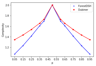
Refer to caption

Figure 5: Comparing the practical performances of Dubiner algorithm in [41] with ForestDSH for S=1000𝑆1000S=1000. ForestDSH outperforms Dubiner’s method for all values of p𝑝p. The pseudo code for the algorithm presented in [41] for the case of hamming distance is generated in this paper in Algorithm 6 in Appendix F.
Observation 1

In this observation, we reformulate the problem of solving (2) to the minimum inner product search problem (MIPS) [35] by transferring the data points from 𝒜Ssuperscript𝒜𝑆\mathcal{A}^{S} and Ssuperscript𝑆\mathcal{B}^{S} to RklSsuperscript𝑅𝑘𝑙𝑆R^{klS} in a way that log((x,y)(x,y))𝑥𝑦𝑥𝑦\log\big{(}\frac{\mathbb{P}(x,y)}{\mathbb{Q}(x,y)}\big{)} is equal to the dot product in this new space. We transformed x𝒜S𝑥superscript𝒜𝑆x\in\mathcal{A}^{S} and yS𝑦superscript𝑆y\in\mathcal{B}^{S} to T(x)klS𝑇𝑥superscript𝑘𝑙𝑆T(x)\in\mathbb{R}^{klS} and T(y)klS𝑇𝑦superscript𝑘𝑙𝑆T(y)\in\mathbb{R}^{klS} as follows:

T(x)𝑇𝑥\displaystyle T(x) =\displaystyle= (fs,i,j),1sS,1ik,1jl,formulae-sequencesubscript𝑓𝑠𝑖𝑗1𝑠𝑆1𝑖𝑘1𝑗𝑙\displaystyle\big{(}f_{s,i,j}\big{)},1\leq s\leq S,1\leq i\leq k,1\leq j\leq l, (69)
fs,i,jsubscript𝑓𝑠𝑖𝑗\displaystyle f_{s,i,j} =\displaystyle= {log(pijqij)ωijif xs=ai0o.w.,\displaystyle\left\{\begin{matrix}\frac{\log\big{(}\frac{p_{ij}}{q_{ij}}\big{)}}{\omega_{ij}}&\mbox{if~{}}x_{s}=a_{i}\\ 0&\mbox{o.w.}\end{matrix}\right., (70)
T(y)𝑇𝑦\displaystyle T(y) =\displaystyle= (gs,i,j),1sS,1ik,1jl,formulae-sequencesubscript𝑔𝑠𝑖𝑗1𝑠𝑆1𝑖𝑘1𝑗𝑙\displaystyle\big{(}g_{s,i,j}\big{)},1\leq s\leq S,1\leq i\leq k,1\leq j\leq l, (71)
gs,i,jsubscript𝑔𝑠𝑖𝑗\displaystyle g_{s,i,j} =\displaystyle= {ωijif ys=bj0o.w..\displaystyle\left\{\begin{matrix}{\omega_{ij}}&\mbox{if~{}}y_{s}=b_{j}\\ 0&\mbox{o.w.}\end{matrix}\right.. (72)

Then, we have log((x,y)(x,y))=<T(x),T(y)>\log\left(\frac{\mathbb{P}(x,y)}{\mathbb{Q}(x,y)}\right)=<T(x),T(y)> where <.,.><.,.> stands for the inner product in klSsuperscript𝑘𝑙𝑆\mathbb{R}^{klS}. In other words, given any x=(x1,,xS)𝑥subscript𝑥1subscript𝑥𝑆x=(x_{1},\cdots,x_{S}), for each xssubscript𝑥𝑠x_{s} we transform it to a kl×1𝑘𝑙1kl\times 1 vector with l𝑙l non-zero elements. Similarly, given any y=(y1,,yS)𝑦subscript𝑦1subscript𝑦𝑆y=(y_{1},\cdots,y_{S}), each yssubscript𝑦𝑠y_{s} is transformed to a kl×1𝑘𝑙1kl\times 1 vector with k𝑘k non-zero elements. Therefore, finding pairs of data points with large (x,y)(x,y)𝑥𝑦𝑥𝑦\frac{\mathbb{P}(x,y)}{\mathbb{Q}(x,y)} is equivalent to finding transformed data points with large dot product. Using this transformation, in Appendix G we show that the angle between both the true pairs and false pairs will be nearly π2𝜋2\frac{\pi}{2} for almost all the probability distributions (S0M20subscript𝑆0superscript𝑀20\frac{S_{0}}{M^{2}}\approx 0, using the notation from [35]). It is well known that MIPS performs poorly in detection of pairs that are nearly orthogonal [35]. Therefore, solving (2) by transforming it to a MIPS problem and using existing approaches fails. Note that, [35] is based on data independent hashes for Euclidean distance that are not the state of the art. Recently, data dependent hashes have been introduced for Euclidean distance that improve on their data independent counterparts [33, 34], while currently there is no data dependent strategy for maximum inner product search. Therefore, MIPS is currently unable to solve (1) efficiently.

Experiment 2

In this experiment, we compared the complexity for the three algorithms LSH-hamming, MinHash and ForestDSH for a range of probability distributions. We benchmark the three methods using matrices P(t)=P1(1t)+P2t𝑃𝑡subscript𝑃11𝑡subscript𝑃2𝑡{P}(t)={P}_{1}(1-t)+{P}_{2}t where 0t10𝑡10\leq t\leq 1, P1=[0.34500.310.345]subscript𝑃1matrix0.34500.310.345{P}_{1}=\begin{bmatrix}0.345&0\\ 0.31&0.345\end{bmatrix}, P2=[0.01962500.0368750.9435]subscript𝑃2matrix0.01962500.0368750.9435{P}_{2}=\begin{bmatrix}0.019625&0\\ 0.036875&0.9435\end{bmatrix}, and δ=1𝛿1\delta=1, i.e., M=N𝑀𝑁M=N. The selection of P1subscript𝑃1{P}_{1} was such that the complexity of MinHash minus the complexity of LSH-hamming was maximized. P2subscript𝑃2{P}_{2} was selected such that the complexity of LSH-hamming minus the complexity of MinHash was maximized. Fig. 6 (a)𝑎(a) shows the theoretical complexities of MinHash, LSH-hamming and ForestDSH for each matrix. See Appendix H, for the details on the derivation of complexities for MinHash, LSH-hamming and ForestDSH. For instance, for P1=[0.34500.310.345]subscript𝑃1matrix0.34500.310.345{P}_{1}=\begin{bmatrix}0.345&0\\ 0.31&0.345\end{bmatrix}, the theoretical per query complexities of MinHash, LSH-hamming and ForestDSH are equal to 0.52070.52070.5207, 0.46720.46720.4672 and 0.43840.43840.4384, respectively. We further consider N𝑁N data points of dimension S𝑆S, {x1,,xN}superscript𝑥1superscript𝑥𝑁\{x^{1},\cdots,x^{N}\} and {y1,,yN}superscript𝑦1superscript𝑦𝑁\{y^{1},\cdots,y^{N}\} where each (xi,yi)superscript𝑥𝑖superscript𝑦𝑖(x^{i},y^{i}) is generated from P(t)𝑃𝑡{P}(t), and xisuperscript𝑥𝑖x^{i} is independent from yjsuperscript𝑦𝑗y^{j} for ij𝑖𝑗i\neq j (N=2000,S=2000)formulae-sequence𝑁2000𝑆2000(N=2000,S=2000). Then, we used ForestDSH, LSH-hamming and MinHash to find the matched pairs. In each case, we tuned #rows#𝑟𝑜𝑤𝑠\#rows666In MinHash and LSH-Hamming, we start with #bands×#rows#𝑏𝑎𝑛𝑑𝑠#𝑟𝑜𝑤𝑠\#bands\times\#rows randomly selected hashes from the family of distribution sensitive hashes, where #rows#𝑟𝑜𝑤𝑠\#rows is the number of rows and #bands#𝑏𝑎𝑛𝑑𝑠\#bands is the number of bands. We recall a pair (x,y)𝑥𝑦(x,y), if x𝑥x and y𝑦y are hashed to the same value in all #rows#𝑟𝑜𝑤𝑠\#rows rows and in at least one of the #bands#𝑏𝑎𝑛𝑑𝑠\#bands bands. and #bands#𝑏𝑎𝑛𝑑𝑠\#bands to achieve 99%percent9999\% true positive (recall) rate. Total simulation time for each of the three methods is plotted for each probability distribution in Figure 6 (b)𝑏(b). The simulation times in Figure 6 (b)𝑏(b) are consistent with the theoretical guarantees in Figure 6 (a)𝑎(a). Figure 6 parts (b)𝑏(b) and (c)𝑐(c) show that for sparse matrices, (t1)𝑡1(t\approx 1), MinHash and ForestDSH outperform LSH-hamming. In denser cases, (t0)𝑡0(t\approx 0), LSH-hamming and ForestDSH outperform MinHash. For (t0.4)𝑡0.4(t\leq 0.4), ForestDSH outperforms both MinHash and LSH-hamming. Note that, for the case when the data is coming from sparse distribution, MinHash beats ForestDSH in practice (as opposed to Theory). This is because for sparse data the total complexity tends to its minimum, i.e., O(N)𝑂𝑁O(N). ForestDSH is inefficient compared to MinHash for small number of N𝑁N and when the data is sparse as the constant terms and logN𝑙𝑜𝑔𝑁logN terms which play a significant role in this case are not optimized in ForestDSH. In Figure 7, we further plotted V(G(N))𝑉𝐺𝑁V(G(N)), α(G(N))β(G(N))𝛼𝐺𝑁𝛽𝐺𝑁\frac{\alpha(G(N))}{\beta(G(N))}, α(G(N))γ𝒜(G(N))𝛼𝐺𝑁superscript𝛾𝒜𝐺𝑁\frac{\alpha(G(N))}{\gamma^{\mathcal{A}}(G(N))} and α(G(N))γ(G(N))𝛼𝐺𝑁superscript𝛾𝐺𝑁\frac{\alpha(G(N))}{\gamma^{\mathcal{B}}(G(N))} as a function of N𝑁N for trees G(N)𝐺𝑁G(N) constructed by Algorithm 4 for P(t=0.25)𝑃𝑡0.25{P}(t=0.25), where M=N𝑀𝑁M=N. As predicted by Theorem 3, we observed that these quantities grow/decay proportional to Nλsuperscript𝑁superscript𝜆N^{\lambda^{*}}, N1+δλsuperscript𝑁1𝛿superscript𝜆N^{1+\delta-\lambda^{*}}, N1λsuperscript𝑁1superscript𝜆N^{1-\lambda^{*}} and Nδλsuperscript𝑁𝛿superscript𝜆N^{\delta-\lambda^{*}}, respectively. In Figure 8, true positive rate and total complexity are plotted in terms of #bands#𝑏𝑎𝑛𝑑𝑠\#bands for the case of N=20,000𝑁20000N=20,000, S=10,000𝑆10000S=10,000 and the probability distribution P2subscript𝑃2{P}_{2}. From (50), i.e., TP=1(1α(G))#bands𝑇𝑃1superscript1𝛼𝐺#𝑏𝑎𝑛𝑑𝑠TP=1-{(1-\alpha(G))}^{\#bands}, we expect true positive rate to increase while #bands#𝑏𝑎𝑛𝑑𝑠\#bands increases (see Figure 8 (a)𝑎(a)). On the other hand, from (51) and (33), total complexity (Nλ)superscript𝑁superscript𝜆(N^{\lambda^{*}}) is expected to linearly increase while #bands#𝑏𝑎𝑛𝑑𝑠\#bands increases (see Figure 8 (b)𝑏(b)).

Refer to caption

(a)𝑎(a)                                    (b)𝑏(b)                                     (c)𝑐(c)

Figure 6: Total (opposed to per query) complexities of LSH-hamming, MinHash, and ForestDSH are plotted for all the probability distribution matrices P(t)=P1(1t)+P2t𝑃𝑡subscript𝑃11𝑡subscript𝑃2𝑡{P}(t)={P}_{1}(1-t)+{P}_{2}t where 0t10𝑡10\leq t\leq 1. (a)𝑎(a) Theoretical guarantees, (b)𝑏(b) Simulation time for N=2000𝑁2000N=2000 and S=2000𝑆2000S=2000, (c)𝑐(c) Simulation time for N=20000𝑁20000N=20000 and S=2000𝑆2000S=2000. Note that ForestDSH performs faster than MinHash if the data is not sparse. While for N=2,000 MinHash is superior to ForestDSH on sparse data, when N=20,000, ForestDSH is performing the same as MinHash. This is mainly due to the fact that constant and logN𝑁\log N terms vanish compared to N𝑁N as N𝑁N grows.

Refer to caption


Figure 7: In this figure, V(G(N))𝑉𝐺𝑁V(G(N)), α(G(N))β(G(N))𝛼𝐺𝑁𝛽𝐺𝑁\frac{\alpha(G(N))}{\beta(G(N))}, α(G(N))γ𝒜(G(N))𝛼𝐺𝑁superscript𝛾𝒜𝐺𝑁\frac{\alpha(G(N))}{\gamma^{\mathcal{A}}(G(N))} and α(G(N))γ(G(N))𝛼𝐺𝑁superscript𝛾𝐺𝑁\frac{\alpha(G(N))}{\gamma^{\mathcal{B}}(G(N))} are depicted as a function of N𝑁N and constants c1subscript𝑐1c_{1}, c2subscript𝑐2c_{2}, c3subscript𝑐3c_{3} and c4subscript𝑐4c_{4} not depending on N𝑁N. The parameters are chosen from Experiment 2. This figure shows how these functions grow/decay proportional to Nλsuperscript𝑁superscript𝜆N^{\lambda^{*}}, N1+δλsuperscript𝑁1𝛿superscript𝜆N^{1+\delta-\lambda^{*}}, N1λsuperscript𝑁1superscript𝜆N^{1-\lambda^{*}} and Nδλsuperscript𝑁𝛿superscript𝜆N^{\delta-\lambda^{*}}, respectively. (See proof of Theorem 3 in Section 6.2 for the justifications. This confirms ((34)-(38)) for trees G(N)𝐺𝑁G(N) constructed by Algorithm 4).

Refer to caption

(a)𝑎(a)                                                                                          (b)𝑏(b)

Figure 8: (a)𝑎(a) True positive rate and (b)𝑏(b) total complexity (Nλ)superscript𝑁superscript𝜆(N^{\lambda^{*}}) are plotted for the probability distribution matrix P2(t)subscript𝑃2𝑡{P}_{2}(t), N=2000𝑁2000N=2000 and S=2000𝑆2000S=2000 in terms of #bands#𝑏𝑎𝑛𝑑𝑠\#bands.
Experiment 3

In this experiment, we examine the robustness of our algorithm from Theorem 4 for matrices considered in Experiment 2 while M=N=300,000formulae-sequence𝑀𝑁300000M=N=300,000. For each P(t)𝑃𝑡{P}(t), we generated random matrices P(t)superscript𝑃𝑡{P}^{\prime}(t) within 1+ϵ1italic-ϵ1+\epsilon of P(t)𝑃𝑡{P}(t), see Theorem 4. We derive the practical complexity and theoretical complexity, i.e., λsuperscript𝜆\lambda^{*} from Definition 4. Moreover, for each of these matrices, we derive the worst case complexity in the case of ϵ=0.03italic-ϵ0.03\epsilon=0.03. This is sketched in Figure 9.

Refer to caption

Figure 9: In this figure, practical, theoretical and noisy complexity are compared for P(t)=P1(1t)+P2t𝑃𝑡subscript𝑃11𝑡subscript𝑃2𝑡{P}(t)={P}_{1}(1-t)+{P}_{2}t given in Experiment 4. Here, M=N=300,000formulae-sequence𝑀𝑁300000M=N=300,000 and the noisy complexity is derived from Theorem 4 with ϵ=0.03italic-ϵ0.03\epsilon=0.03.
Experiment 4

In this experiment, we used the mass spectral data from human microbiome [43], extracted using MSCluster [1]. In this problem, there are N𝑁N spectra X=x1,,xN𝑋superscript𝑥1superscript𝑥𝑁X={x^{1},\cdots,x^{N}}, and a query spectrum y𝑦y. Our goal is to find the spectra xisuperscript𝑥𝑖x^{i} that maximize a probabilistic model (y|xi)conditional𝑦superscript𝑥𝑖\mathbb{P}(y|x^{i}). (y|x)conditional𝑦𝑥\mathbb{P}(y|x) is learned assuming that it can be factorized to i.i.d. components. To learn p(yx)𝑝conditional𝑦𝑥p(y\mid x), each mass spectra is sorted based on the peak intensities, and in order to reduce the number of parameters we need to learn, instead of the peak ranks we use log of the peak ranks 777logbRanksubscript𝑏𝑅𝑎𝑛𝑘\log_{b}Rank of a peak is defined as the logbsubscript𝑏\log_{b} of its rank𝑟𝑎𝑛𝑘rank. For any natural number n𝑛n, logbRank=nsubscript𝑏𝑅𝑎𝑛𝑘𝑛\log_{b}Rank=n for the peaks at rank {bn1,,bn1}superscript𝑏𝑛1superscript𝑏𝑛1\{b^{n-1},\cdots,b^{n}-1\}, e.g., log2Rank(m)=3subscript2𝑅𝑎𝑛𝑘𝑚3\log_{2}Rank(m)=3 for m{4,5,6,7}𝑚4567m\in\{4,5,6,7\}. Joint probability distribution of logRanks for the data from [1] is shown in Figures 10 (a)𝑎(a) (4×4444\times 4 data matrix is obtained using log4Ranksubscript4𝑅𝑎𝑛𝑘\log_{4}Rank), (b)𝑏(b) (8×8888\times 8 data matrix is obtained using log2Ranksubscript2𝑅𝑎𝑛𝑘\log_{2}Rank) and (c)𝑐(c) (51×51515151\times 51 data matrix is obtained not using any logbRanksubscript𝑏𝑅𝑎𝑛𝑘\log_{b}Rank).. Using these data, we learn the joint probability distribution p(logRank(ys)=ilogRank(xs)=j)𝑝𝑅𝑎𝑛𝑘subscript𝑦𝑠conditional𝑖𝑅𝑎𝑛𝑘subscript𝑥𝑠𝑗p(\log Rank(y_{s})=i\mid\log Rank(x_{s})=j). Among 90753 data points, we used 70753 for training, and 20000 for the test. The joint probability distribution of matching pairs are shown in Figures 10, before and after logRank transformation.

After learning this probabilistic model, we applied ForestDSH method to the test mass spectra (after logRank𝑅𝑎𝑛𝑘\log Rank transformation), and we were able to speed up the search of 200002000020000 mass spectra nine times, in comparison to brute force search while maintaining true positive rate of 90%percent9090\%. For ForestDSH method, the total runtime is 705,197ms705197𝑚𝑠705,197ms, while for brute force, the total runtime is 6,022,373ms (eight times slower than ForestDSH), and for LSH, the runtime for achieving 90%percent9090\% TP rate is 5,495,518ms (seven times slower than ForestDSH). The amount of memory used peaks at 220MB.

Refer to caption

(a)𝑎(a)                                   (b)𝑏(b)                                    (c)𝑐(c)

Figure 10: Mass spectrometry joint probability distribution in the case of (a)𝑎(a) log4Ranksubscript4𝑅𝑎𝑛𝑘\log_{4}Rank, (b)𝑏(b) log2Ranksubscript2𝑅𝑎𝑛𝑘\log_{2}Rank, and (c)𝑐(c) no logRank𝑅𝑎𝑛𝑘\log Rank filter. For further details on mass spectrometry joint probability distributions, see Appendix I.
Experiment 5

In this experiment, we considered a set of 50,0005000050,000 images (25,0002500025,000 pairs of images) from CIFAR-10 database [44]. Each pair of images consists of a grey-scale 3232323232*32 pixels image and a noisy version of the image constructed by adding independent Gaussian noise 𝒩(μ=0.5,σ=0.039)𝒩formulae-sequence𝜇0.5𝜎0.039\mathcal{N}(\mu=0.5,\sigma=0.039) and discretizing pixels to binary. ForestDSH is able to detect true pairs with the success rate of 99%percent9999\% in 1,970 seconds while brute force approach detects true pairs in 19,123 seconds (nine times slower than ForestDSH) and LSH detects true pairs within 15,080 seconds (seven times slower than ForestDSH).
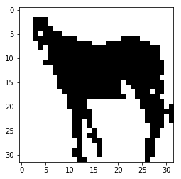
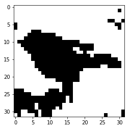
Refer to captionRefer to captionRefer to captionRefer to captionRefer to caption

+𝒩(μ,σ)absent𝒩𝜇𝜎\downarrow+\mathcal{N}(\mu,\sigma)         +𝒩(μ,σ)absent𝒩𝜇𝜎\downarrow+\mathcal{N}(\mu,\sigma)          +𝒩(μ,σ)absent𝒩𝜇𝜎\downarrow+\mathcal{N}(\mu,\sigma)         +𝒩(μ,σ)absent𝒩𝜇𝜎\downarrow+\mathcal{N}(\mu,\sigma)         +𝒩(μ,σ)absent𝒩𝜇𝜎\downarrow+\mathcal{N}(\mu,\sigma)

Refer to captionRefer to captionRefer to captionRefer to captionRefer to caption
Figure 11: In this figure, five grey-scale 3232323232*32 pixels images along with their noisy versions are shown. Here, ForestDSH is able to detect true pairs with the success rate of 99%percent9999\% while being nine times faster than brute force and seven times faster than LSH.

7.1 Codes

For the codes, see https://github.com/mohimanilab/ForestDSH.

8 Conclusion

ForestDSH algorithm proposed in this paper is comprehensive and efficient in the sense that for a wide range of probability distributions it enables us to capture the difference between pairs coming from a joint probability distributions and independent pairs. This algorithm is built upon a family of distribution sensitive hashes and is designed using a decision tree structure which is constructed recursively. Moreover, we prove that the decision tree introduced here has a complexity of O(Nλ)𝑂superscript𝑁superscript𝜆O(N^{\lambda^{*}}) and there is no decision tree with overall complexity below it. We prove that this algorithm outperforms existing state of the art approaches in specific range of distributions, in theory and practice and enabled speeding up the spectral library search in mass spectrometry by a factor of nine. Finally, we should note that ForestDSH has some limitations which are discussed as follows. ForestDSH assumes that the probability distribution function is factorizable to i.i.d. components. Generalizing ForestDSH to the case of general probability distribution function is an open problem and our results here open a path towards solving the general probability mass function problem. Moreover, the special case of factorizable models are simple but crucial models that have been widely used in computational biology, e.g., see [3], and other areas of data sciences. In the future, we will address the more general problem of Markov chain models. Note that ForestDSH performs faster than MinHash if the data is not sparse. While for a small number of datapoints MinHash is superior to ForestDSH on sparse data, for a larger number of datapoints ForestDSH is performing the same as MinHash. This is mainly due to the fact that constant and logarithmic terms vanish in ratio as the number of datapoints grows.

References

  • [1] A. M. Frank, M. E. Monroe, A. R. Shah, J. J. Carver, N. Bandeira, R. J. Moore, G. A. Anderson, R. D. Smith, and P. A. Pevzner, “Spectral archives: extending spectral libraries to analyze both identified and unidentified spectra,” Nature methods, vol. 8, no. 7, p. 587, 2011.
  • [2] R. Aebersold and M. Mann, “Mass spectrometry-based proteomics,” Nature, vol. 422, no. 6928, p. 198, 2003.
  • [3] S. Kim and P. A. Pevzner, “MS-GF+ makes progress towards a universal database search tool for proteomics,” Nature communications, vol. 5, p. 5277, 2014.
  • [4] B. V. Dasarathy and B. V. Sheela, “Visiting nearest neighbors-a survery of nearest neighbor pattern classification techniques,” in Proceedings of the international conference on cybernetics and society, pp. 630–636, 1977.
  • [5] P. N. Yianilos, “Data structures and algorithms for nearest neighbor search in general metric spaces,” in Soda, vol. 93, no. 194, pp. 311–21, 1993.
  • [6] R. O. Duda, P. E. Hart et al., Pattern classification and scene analysis.   Wiley New York, vol. 3, 1973.
  • [7] A. Guttman, “R-trees: A dynamic index structure for spatial searching,” in Proceedings of the 1984 ACM SIGMOD international conference on Management of data, pp. 47–57, 1984.
  • [8] G. Mori, S. Belongie, and J. Malik, “Shape contexts enable efficient retrieval of similar shapes,” in Proceedings of the 2001 IEEE Computer Society Conference on Computer Vision and Pattern Recognition. CVPR 2001, vol. 1, pp. I–I, 2001.
  • [9] G. Shakhnarovich, P. Viola, and T. Darrell, “Fast pose estimation with parameter-sensitive hashing,” in IEEE International Conference on Computer Vision-Volume 2, p. 750, 2003.
  • [10] J. L. Bentley, “Multidimensional binary search trees used for associative searching,” Communications of the ACM, vol. 18, no. 9, pp. 509–517, 1975.
  • [11] Y. Prabhu and M. Varma, “Fastxml: A fast, accurate and stable tree-classifier for extreme multi-label learning,” in Proceedings of the 20th ACM SIGKDD international conference on Knowledge discovery and data mining, pp. 263–272, 2014.
  • [12] J. Friedman, J. Bentley, and R. Finkel, “An algorithm for finding best matches in logarithmic time,” ACM Trans. Math. Software, 3(SLAC-PUB-1549-REV. 2, pp. 209–226, 1976.
  • [13] H. Jain, Y. Prabhu, and M. Varma, “Extreme multi-label loss functions for recommendation, tagging, ranking & other missing label applications,” in Proceedings of the 22nd ACM SIGKDD International Conference on Knowledge Discovery and Data Mining.   ACM, pp. 935–944, 2016.
  • [14] K. Bhatia, H. Jain, P. Kar, M. Varma, and P. Jain, “Sparse local embeddings for extreme multi-label classification,” in Advances in neural information processing systems, pp. 730–738, 2015.
  • [15] I. E.-H. Yen, X. Huang, P. Ravikumar, K. Zhong, and I. Dhillon, “Pd-sparse: A primal and dual sparse approach to extreme multiclass and multilabel classification,” in International Conference on Machine Learning, pp. 3069–3077, 2016.
  • [16] A. E. Choromanska and J. Langford, “Logarithmic time online multiclass prediction,” in Advances in Neural Information Processing Systems, pp. 55–63, 2015.
  • [17] W. Liu and I. W. Tsang, “Making decision trees feasible in ultrahigh feature and label dimensions,” The Journal of Machine Learning Research, vol. 18, no. 1, pp. 2814–2849, 2017.
  • [18] J. Nam, E. L. Mencía, H. J. Kim, and J. Fürnkranz, “Maximizing subset accuracy with recurrent neural networks in multi-label classification,” in Advances in neural information processing systems, pp. 5413–5423, 2017.
  • [19] P. Rai, C. Hu, R. Henao, and L. Carin, “Large-scale bayesian multi-label learning via topic-based label embeddings,” in Advances in Neural Information Processing Systems, pp. 3222–3230, 2015.
  • [20] Y. Tagami, “Annexml: Approximate nearest neighbor search for extreme multi-label classification,” in Proceedings of the 23rd ACM SIGKDD international conference on knowledge discovery and data mining.   ACM, pp. 455–464, 2017.
  • [21] A. Niculescu-Mizil and E. Abbasnejad, “Label filters for large scale multilabel classification,” in Artificial Intelligence and Statistics, pp. 1448–1457, 2017.
  • [22] W.-J. Zhou, Y. Yu, and M.-L. Zhang, “Binary linear compression for multi-label classification.” in IJCAI, pp. 3546–3552, 2017.
  • [23] K. Beyer, J. Goldstein, R. Ramakrishnan, and U. Shaft, “When is “nearest neighbor” meaningful?” in International conference on database theory.   Springer, pp. 217–235, 1999.
  • [24] V. Castelli, C.-S. Li, and A. Thomasian, “Searching multidimensional indexes using associated clustering and dimension reduction information,” Oct. 17, US Patent 6,134,541, 2000.
  • [25] E. Anagnostopoulos, I. Z. Emiris, and I. Psarros, “Low-quality dimension reduction and high-dimensional approximate nearest neighbor,” in 31st International Symposium on Computational Geometry (SoCG 2015).   Schloss Dagstuhl-Leibniz-Zentrum fuer Informatik, 2015.
  • [26] R. Min, A non-linear dimensionality reduction method for improving nearest neighbour classification.   University of Toronto, 2005.
  • [27] B. Shaw and T. Jebara, “Structure preserving embedding,” in Proceedings of the 26th Annual International Conference on Machine Learning, pp. 937–944, 2009.
  • [28] T. Christiani and R. Pagh, “Set similarity search beyond minhash,” in Proceedings of the 49th Annual ACM SIGACT Symposium on Theory of Computing.   ACM, pp. 1094–1107, 2017.
  • [29] M. S. Charikar, “Similarity estimation techniques from rounding algorithms,” in Proceedings of the thirty-fourth annual ACM symposium on Theory of computing.   ACM, pp. 380–388, 2002.
  • [30] P. Indyk and R. Motwani, “Approximate nearest neighbors: towards removing the curse of dimensionality,” in Proceedings of the thirtieth annual ACM symposium on Theory of computing, pp. 604–613, 1998.
  • [31] A. Gionis, P. Indyk, R. Motwani et al., “Similarity search in high dimensions via hashing,” in Vldb, vol. 99, no. 6, pp. 518–529, 1999.
  • [32] M. Bawa, T. Condie, and P. Ganesan, “LSH forest: self-tuning indexes for similarity search,” in Proceedings of the 14th international conference on World Wide Web, pp. 651–660, 2005.
  • [33] A. Andoni, T. Laarhoven, I. Razenshteyn, and E. Waingarten, “Optimal hashing-based time-space trade-offs for approximate near neighbors,” in Proceedings of the Twenty-Eighth Annual ACM-SIAM Symposium on Discrete Algorithms.   Society for Industrial and Applied Mathematics, pp. 47–66, 2017.
  • [34] A. Rubinstein, “Hardness of approximate nearest neighbor search,” in Proceedings of the 50th Annual ACM SIGACT Symposium on Theory of Computing.   ACM, pp. 1260–1268, 2018.
  • [35] A. Shrivastava and P. Li, “Asymmetric lsh (alsh) for sublinear time maximum inner product search (mips),” in Advances in Neural Information Processing Systems, pp. 2321–2329, 2014.
  • [36] A. Andoni and I. Razenshteyn, “Optimal data-dependent hashing for approximate near neighbors,” in Proceedings of the forty-seventh annual ACM symposium on Theory of computing.   ACM, pp. 793–801, 2015.
  • [37] A. Andoni, P. Indyk, T. Laarhoven, I. Razenshteyn, and L. Schmidt, “Practical and optimal lsh for angular distance,” in Advances in Neural Information Processing Systems, pp. 1225–1233, 2015.
  • [38] A. Chakrabarti and O. Regev, “An optimal randomized cell probe lower bound for approximate nearest neighbor searching,” SIAM Journal on Computing, vol. 39, no. 5, pp. 1919–1940, 2010.
  • [39] P. B. Miltersen, “Cell probe complexity-a survey,” in Proceedings of the 19th Conference on the Foundations of Software Technology and Theoretical Computer Science, Advances in Data Structures Workshop, p. 2, 1999.
  • [40] A. Andoni, A. Naor, A. Nikolov, I. Razenshteyn, and E. Waingarten, “Data-dependent hashing via nonlinear spectral gaps,” in Proceedings of the 50th Annual ACM SIGACT Symposium on Theory of Computing.   ACM, pp. 787–800, 2018.
  • [41] M. Dubiner, “A heterogeneous high-dimensional approximate nearest neighbor algorithm,” IEEE Transactions on Information Theory, vol. 58, no. 10, pp. 6646–6658, 2012.
  • [42] ——, “Bucketing coding and information theory for the statistical high-dimensional nearest-neighbor problem,” IEEE Transactions on Information Theory, vol. 56, no. 8, pp. 4166 – 4179, Aug 2010.
  • [43] D. McDonald, E. Hyde, J. W. Debelius, J. T. Morton, A. Gonzalez, G. Ackermann, A. A. Aksenov, B. Behsaz, C. Brennan, Y. Chen et al., “American gut: an open platform for citizen science microbiome research,” MSystems, vol. 3, no. 3, pp. e00 031–18, 2018.
  • [44] A. Krizhevsky, G. Hinton et al., “Learning multiple layers of features from tiny images,” 2009.

Appendix A Proof of Lemmas 1 and 2

A.1 Proof of Lemma 1.

Lemma 1 is proved by induction on the depth of the node v𝑣v. For example, consider v𝑣v and its children wij=f(v,ai,bj)subscript𝑤𝑖𝑗𝑓𝑣subscript𝑎𝑖subscript𝑏𝑗w_{ij}=f(v,a_{i},b_{j}). From (21), we have Φ(wij)=Φ(v)pijΦsubscript𝑤𝑖𝑗Φ𝑣subscript𝑝𝑖𝑗\Phi(w_{ij})=\Phi(v)p_{ij}. Therefore, (25) is proved by induction as follows. Assume (25) holds for any node with depth less than d𝑑d. Consider the node wijsubscript𝑤𝑖𝑗w_{ij} which is a children of v𝑣v, i.e., wij=f(v,ai,bj)subscript𝑤𝑖𝑗𝑓𝑣subscript𝑎𝑖subscript𝑏𝑗w_{ij}=f(v,a_{i},b_{j}) and depth(wij)=d𝑑𝑒𝑝𝑡subscript𝑤𝑖𝑗𝑑depth(w_{ij})=d.

Φ(wij)Φsubscript𝑤𝑖𝑗\displaystyle\Phi(w_{ij}) =\displaystyle= Φ(v)pijΦ𝑣subscript𝑝𝑖𝑗\displaystyle\Phi(v)p_{ij} (73)
=\displaystyle= Prob(vHz𝒜(x)Hz(y)(x,y))pij𝑃𝑟𝑜𝑏𝑣superscriptsubscript𝐻𝑧𝒜𝑥conditionalsuperscriptsubscript𝐻𝑧𝑦𝑥𝑦similar-tosubscript𝑝𝑖𝑗\displaystyle Prob(v\in H_{z}^{\mathcal{A}}(x)\cap H_{z}^{\mathcal{B}}(y)\mid(x,y)\sim\mathbb{P})p_{ij}
=\displaystyle= Prob(Seq𝒜(v) is a prefix of permz(x)\displaystyle Prob(Seq^{\mathcal{A}}(v)\mbox{~{}is a prefix of perm}_{z}(x)
,Seq(v) is a prefix of permz(y)(x,y))pij\displaystyle,Seq^{\mathcal{B}}(v)\mbox{~{}is a prefix of perm}_{z}(y)\mid(x,y)\sim\mathbb{P})p_{ij}
=\displaystyle= Prob(Seq𝒜(v) is a prefix of permz(x)\displaystyle Prob(Seq^{\mathcal{A}}(v)\mbox{~{}is a prefix of perm}_{z}(x)
,Seq(v) is a prefix of permz(y),ai=(permz(x))d,bj=(permz(y))d(x,y))\displaystyle,Seq^{\mathcal{B}}(v)\mbox{~{}is a prefix of perm}_{z}(y),a_{i}={({perm_{z}}(x))}_{d},b_{j}={\color[rgb]{0,0,0}{({perm_{z}}(y))}_{d}}\mid(x,y)\sim\mathbb{P})
=\displaystyle= Prob(wijHz𝒜(x)Hz(y)(x,y)).𝑃𝑟𝑜𝑏subscript𝑤𝑖𝑗superscriptsubscript𝐻𝑧𝒜𝑥conditionalsuperscriptsubscript𝐻𝑧𝑦𝑥𝑦similar-to\displaystyle Prob(w_{ij}\in H_{z}^{\mathcal{A}}(x)\cap H_{z}^{\mathcal{B}}(y)\mid(x,y)\sim\mathbb{P}). (77)

See Section 4 for the Definition of permz𝑝𝑒𝑟subscript𝑚𝑧perm_{z}. Note that (permz(x))dsubscript𝑝𝑒𝑟subscript𝑚𝑧𝑥𝑑{({perm_{z}}(x))}_{d} stands for d𝑑d-th entry of the vector (permz(x))𝑝𝑒𝑟subscript𝑚𝑧𝑥{({perm_{z}}(x))}. (A.1) follows from induction assumption for the nodes with depth less than d𝑑d, (LABEL:tp3) is a result of i.i.d. assumption (2), i.e., (yx)=s=1Sp(ysxs)conditional𝑦𝑥superscriptsubscriptproduct𝑠1𝑆𝑝conditionalsubscript𝑦𝑠subscript𝑥𝑠\mathbb{P}(y\mid x)=\prod_{s=1}^{S}p(y_{s}\mid x_{s}) and the defnition of Hz𝒜(x)superscriptsubscript𝐻𝑧𝒜𝑥H_{z}^{\mathcal{A}}(x) in (19). ((26)(28))italic-(26italic-)italic-(28italic-)(\eqref{famm1}-\eqref{fam2}) follow similarly.

A.2 Proof of Lemma 2.

Using ((25)(28))italic-(25italic-)italic-(28italic-)(\eqref{fam1}-\eqref{fam2}), constraints ((11)(15))italic-(11italic-)italic-(15italic-)(\eqref{family1}-\eqref{family2}) hold for α=α(G)𝛼𝛼𝐺\alpha=\alpha(G), β=β(G)𝛽𝛽𝐺\beta=\beta(G), γ𝒜=γ𝒜(G)superscript𝛾𝒜superscript𝛾𝒜𝐺\gamma^{\mathcal{A}}=\gamma^{\mathcal{A}}(G) and γ=γ(G)superscript𝛾superscript𝛾𝐺\gamma^{\mathcal{B}}=\gamma^{\mathcal{B}}(G). Since no two buckets are ancestor/descendant of each other, we have

H𝒜(x)H(y)1.delimited-∣∣superscript𝐻𝒜𝑥superscript𝐻𝑦1\displaystyle{\mid H^{\mathcal{A}}(x)\cap H^{\mathcal{B}}(y)\mid}\leq 1. (78)

Therefore, (15) holds. This completes the proof that Hz𝒜(x)superscriptsubscript𝐻𝑧𝒜𝑥H_{z}^{\mathcal{A}}(x) and Hz(y)superscriptsubscript𝐻𝑧𝑦H_{z}^{\mathcal{B}}(y) defined in (19) and (20) are
(α(G),β(G),γ𝒜(G),γ(G))𝛼𝐺𝛽𝐺superscript𝛾𝒜𝐺superscript𝛾𝐺(\alpha(G),\beta(G),\gamma^{\mathcal{A}}(G),\gamma^{\mathcal{B}}(G))-sensitive.

Appendix B Deriving μsuperscript𝜇\mu^{*}, νsuperscript𝜈\nu^{*}, ηsuperscript𝜂\eta^{*}, λsuperscript𝜆\lambda^{*}, p0subscript𝑝0p_{0}, q0subscript𝑞0q_{0} and δ𝛿\delta for \mathbb{P}, M𝑀M and N𝑁N

In this section, an algorithm for deriving μsuperscript𝜇\mu^{*}, νsuperscript𝜈\nu^{*}, ηsuperscript𝜂\eta^{*}, λsuperscript𝜆\lambda^{*}, p0subscript𝑝0p_{0}, q0subscript𝑞0q_{0} and δ𝛿\delta for \mathbb{P}, M𝑀M and N𝑁N for the probability distribution \mathbb{P} and δ𝛿\delta is presented for a given probability distribution \mathbb{P}.

Algorithm 5 Deriving μsuperscript𝜇\mu^{*}, νsuperscript𝜈\nu^{*}, ηsuperscript𝜂\eta^{*}, λsuperscript𝜆\lambda^{*}, p0subscript𝑝0p_{0}, q0subscript𝑞0q_{0} and δ𝛿\delta for \mathbb{P}, M𝑀M and N𝑁N
  Inputs: The probability distribution \mathbb{P}, listμ𝑙𝑖𝑠subscript𝑡𝜇{list}_{\mu}, listν𝑙𝑖𝑠subscript𝑡𝜈{list}_{\nu}, listη𝑙𝑖𝑠subscript𝑡𝜂{list}_{\eta}, threshold T𝑇T, M𝑀M and N𝑁N.
  Outputs: μsuperscript𝜇\mu^{*}, νsuperscript𝜈\nu^{*}, ηsuperscript𝜂\eta^{*}, λsuperscript𝜆\lambda^{*}, p0subscript𝑝0p_{0}, q0subscript𝑞0q_{0} and δ𝛿\delta.
  Procedure
      δlogMlogN𝛿𝑀𝑁\delta\leftarrow\frac{\log M}{\log N}
      λ=0superscript𝜆0\lambda^{*}=0
      For μlistμ𝜇𝑙𝑖𝑠subscript𝑡𝜇\mu\in{list}_{\mu}    ##\# For some set of listμ𝑙𝑖𝑠subscript𝑡𝜇{list}_{\mu}, e.g., {0,0.1,0.2,,10}00.10.210\{0,0.1,0.2,\cdots,10\}.
          For νlistν𝜈𝑙𝑖𝑠subscript𝑡𝜈\nu\in{list}_{\nu}   ##\# For some set of listν𝑙𝑖𝑠subscript𝑡𝜈{list}_{\nu}, e.g., {0,0.1,0.2,,10}00.10.210\{0,0.1,0.2,\cdots,10\}.
              For ηlistη𝜂𝑙𝑖𝑠subscript𝑡𝜂\eta\in{list}_{\eta}   ##\# For some set of listη𝑙𝑖𝑠subscript𝑡𝜂{list}_{\eta}, e.g., {0,0.1,0.2,,10}00.10.210\{0,0.1,0.2,\cdots,10\}.
                  If |i,jpij1+μ+νη(pi𝒜)μ(pj)ν1|Tsubscript𝑖𝑗superscriptsubscript𝑝𝑖𝑗1𝜇𝜈𝜂superscriptsuperscriptsubscript𝑝𝑖𝒜𝜇superscriptsuperscriptsubscript𝑝𝑗𝜈1𝑇|\sum_{i,j}p_{ij}^{1+\mu+\nu-\eta}{(p_{i}^{\mathcal{A}})}^{-\mu}{(p_{j}^{\mathcal{B}})}^{-\nu}-1|\leq T and max(1,δ)+μ+δν1+μ+νη>λ1𝛿𝜇𝛿𝜈1𝜇𝜈𝜂superscript𝜆\frac{\max(1,\delta)+\mu+\delta\nu}{1+\mu+\nu-\eta}>\lambda^{*}. ##\# For some small threshold T𝑇T, e.g., 0.0010.0010.001
                      μμsuperscript𝜇𝜇\mu^{*}\leftarrow\mu, ννsuperscript𝜈𝜈\nu^{*}\leftarrow\nu, ηηsuperscript𝜂𝜂\eta^{*}\leftarrow\eta, λmax(1,δ)+μ+δν1+μ+νηsuperscript𝜆1𝛿𝜇𝛿𝜈1𝜇𝜈𝜂\lambda^{*}\leftarrow\frac{\max(1,\delta)+\mu+\delta\nu}{1+\mu+\nu-\eta}
      #p0subscript𝑝0p_{0}, q0subscript𝑞0q_{0} are computed as follows.
      p01subscript𝑝01p_{0}\leftarrow 1, q01subscript𝑞01q_{0}\leftarrow 1, p0𝒜1superscriptsubscript𝑝0𝒜1p_{0}^{\mathcal{A}}\leftarrow 1, p01superscriptsubscript𝑝01p_{0}^{\mathcal{B}}\leftarrow 1
      For ai𝒜subscript𝑎𝑖𝒜a_{i}\in\mathcal{A}
          For bjsubscript𝑏𝑗b_{j}\in\mathcal{B}
              p0p0pijsubscript𝑝0subscript𝑝0subscript𝑝𝑖𝑗p_{0}\leftarrow p_{0}p_{ij}
              q0q0qijsubscript𝑞0subscript𝑞0subscript𝑞𝑖𝑗q_{0}\leftarrow q_{0}q_{ij}
              p0𝒜p0𝒜pi𝒜superscriptsubscript𝑝0𝒜superscriptsubscript𝑝0𝒜superscriptsubscript𝑝𝑖𝒜p_{0}^{\mathcal{A}}\leftarrow p_{0}^{\mathcal{A}}p_{i}^{\mathcal{A}}
              p0p0pjsuperscriptsubscript𝑝0superscriptsubscript𝑝0superscriptsubscript𝑝𝑗p_{0}^{\mathcal{B}}\leftarrow p_{0}^{\mathcal{B}}p_{j}^{\mathcal{B}}
      q0min(q0,p0𝒜,p0)subscript𝑞0subscript𝑞0superscriptsubscript𝑝0𝒜superscriptsubscript𝑝0q_{0}\leftarrow\min(q_{0},p_{0}^{\mathcal{A}},p_{0}^{\mathcal{B}}).
Remark 8

In Algorithm 5, the parameters μsuperscript𝜇\mu^{*}, νsuperscript𝜈\nu^{*}, ηsuperscript𝜂\eta^{*} and λsuperscript𝜆\lambda^{*} could be derived from newton method too.

Appendix C Proof of Theorem 2

In order to prove Theorem 2, we first state the following two lemmas.

Lemma 3

The function f(θ,θ1,θ2,θ3)=θ1+ρ1+ρ2+ρ3θ1ρ1θ2ρ2θ3ρ3𝑓𝜃subscript𝜃1subscript𝜃2subscript𝜃3superscript𝜃1subscript𝜌1subscript𝜌2subscript𝜌3superscriptsubscript𝜃1subscript𝜌1superscriptsubscript𝜃2subscript𝜌2superscriptsubscript𝜃3subscript𝜌3f(\theta,\theta_{1},\theta_{2},\theta_{3})={\theta}^{1+\rho_{1}+\rho_{2}+\rho_{3}}{\theta_{1}}^{-\rho_{1}}{\theta_{2}}^{-\rho_{2}}{\theta_{3}}^{-\rho_{3}} is a convex function on the region (θ,θ1,θ2,θ3)4+𝜃subscript𝜃1subscript𝜃2subscript𝜃3superscriptlimit-from4(\theta,\theta_{1},\theta_{2},\theta_{3})\in\mathbb{R}^{4+} where (ρ1,ρ2,ρ3)3+subscript𝜌1subscript𝜌2subscript𝜌3superscriptlimit-from3(\rho_{1},\rho_{2},\rho_{3})\in\mathbb{R}^{3+}. 888For any natural number n𝑛n, n+superscriptlimit-from𝑛\mathbb{R}^{n+} denotes as the set of all n𝑛n-tuples non-negative real numbers.

Lemma 4

vVBuckets(G)(Φ(v))1+μ+νη(Ψ𝒜(v))μ+η(Ψ(v))ν+η(Ψ(v))η1subscript𝑣subscript𝑉𝐵𝑢𝑐𝑘𝑒𝑡𝑠𝐺superscriptΦ𝑣1𝜇𝜈𝜂superscriptsuperscriptΨ𝒜𝑣𝜇𝜂superscriptsuperscriptΨ𝑣𝜈𝜂superscriptΨ𝑣𝜂1\sum_{v\in V_{Buckets}(G)}{\big{(}\Phi(v)\big{)}}^{1+\mu+\nu-\eta}{\big{(}{\Psi}^{\mathcal{A}}(v)\big{)}}^{-\mu+\eta}{\big{(}{\Psi}^{\mathcal{B}}(v)\big{)}}^{-\nu+\eta}{\big{(}\Psi(v)\big{)}}^{-\eta}\leq 1 for any (μ,ν,η)𝜇𝜈𝜂(\mu,\nu,\eta)\in\mathcal{I}.

Proof of Lemma 3 and Lemma 4, are relegated to Appendices C.1 and C.2, respectively. Consider (μ,ν,η)superscript𝜇superscript𝜈superscript𝜂(\mu^{*},\nu^{*},\eta^{*}) that satisfy (53). For any decision tree satisfying ((34)(38))italic-(34italic-)italic-(38italic-)(\eqref{order1}-\eqref{order3}), we have:

(vVBuckets(G)Φ(v)|VBuckets(G)|)1+μ+νη(vVBuckets(G)Ψ𝒜(v)|VBuckets(G)|)μ+ηsuperscriptsubscript𝑣subscript𝑉𝐵𝑢𝑐𝑘𝑒𝑡𝑠𝐺Φ𝑣subscript𝑉𝐵𝑢𝑐𝑘𝑒𝑡𝑠𝐺1superscript𝜇superscript𝜈superscript𝜂superscriptsubscript𝑣subscript𝑉𝐵𝑢𝑐𝑘𝑒𝑡𝑠𝐺superscriptΨ𝒜𝑣subscript𝑉𝐵𝑢𝑐𝑘𝑒𝑡𝑠𝐺superscript𝜇superscript𝜂\displaystyle{(\frac{\sum_{v\in V_{Buckets}(G)}{\Phi(v)}}{|V_{Buckets}(G)|})}^{1+\mu^{*}+\nu^{*}-\eta^{*}}{(\frac{\sum_{v\in V_{Buckets}(G)}{{\Psi}^{\mathcal{A}}(v)}}{|V_{Buckets}(G)|})}^{-\mu^{*}+\eta^{*}} (79)
×(vVBuckets(G)Ψ(v)|VBuckets(G)|)ν+η(vVBuckets(G)Ψ(v)|VBuckets(G)|)ηabsentsuperscriptsubscript𝑣subscript𝑉𝐵𝑢𝑐𝑘𝑒𝑡𝑠𝐺superscriptΨ𝑣subscript𝑉𝐵𝑢𝑐𝑘𝑒𝑡𝑠𝐺superscript𝜈superscript𝜂superscriptsubscript𝑣subscript𝑉𝐵𝑢𝑐𝑘𝑒𝑡𝑠𝐺Ψ𝑣subscript𝑉𝐵𝑢𝑐𝑘𝑒𝑡𝑠𝐺superscript𝜂\displaystyle\times{(\frac{\sum_{v\in V_{Buckets}(G)}{{\Psi}^{\mathcal{B}}(v)}}{|V_{Buckets}(G)|})}^{-\nu^{*}+\eta^{*}}{(\frac{\sum_{v\in V_{Buckets}(G)}{\Psi(v)}}{|V_{Buckets}(G)|})}^{-\eta^{*}}
\displaystyle\leq vVBuckets(G)(Φ(v))1+μ+νη(Ψ𝒜(v))μ+η(Ψ(v))ν+η(Ψ(v))η|VBuckets(G)|subscript𝑣subscript𝑉𝐵𝑢𝑐𝑘𝑒𝑡𝑠𝐺superscriptΦ𝑣1superscript𝜇superscript𝜈superscript𝜂superscriptsuperscriptΨ𝒜𝑣superscript𝜇superscript𝜂superscriptsuperscriptΨ𝑣superscript𝜈superscript𝜂superscriptΨ𝑣superscript𝜂subscript𝑉𝐵𝑢𝑐𝑘𝑒𝑡𝑠𝐺\displaystyle\frac{\sum_{v\in V_{Buckets}(G)}{\big{(}\Phi(v)\big{)}}^{1+\mu^{*}+\nu^{*}-\eta^{*}}{\big{(}{\Psi}^{\mathcal{A}}(v)\big{)}}^{-\mu^{*}+\eta^{*}}{\big{(}{\Psi}^{\mathcal{B}}(v)\big{)}}^{-\nu^{*}+\eta^{*}}{\big{(}\Psi(v)\big{)}}^{-\eta^{*}}}{|V_{Buckets}(G)|}
\displaystyle\leq 1|VBuckets(G)|,1subscript𝑉𝐵𝑢𝑐𝑘𝑒𝑡𝑠𝐺\displaystyle\frac{1}{|V_{Buckets}(G)|}, (80)

where (79) holds to the convexity of f(θ,θ1,θ2,θ3)=θ1+ρ1+ρ2+ρ3θ1ρ1θ2ρ2θ3ρ3𝑓𝜃subscript𝜃1subscript𝜃2subscript𝜃3superscript𝜃1subscript𝜌1subscript𝜌2subscript𝜌3superscriptsubscript𝜃1subscript𝜌1superscriptsubscript𝜃2subscript𝜌2superscriptsubscript𝜃3subscript𝜌3f(\theta,\theta_{1},\theta_{2},\theta_{3})={\theta}^{1+\rho_{1}+\rho_{2}+\rho_{3}}{\theta_{1}}^{-\rho_{1}}{\theta_{2}}^{-\rho_{2}}{\theta_{3}}^{-\rho_{3}} in Lemma 3 and (80) follows from Lemma 4. Therefore, we have

(vVBuckets(G)Φ(v))1+μ+νη(vVBuckets(G)Ψ𝒜(v))μ+ηsuperscriptsubscript𝑣subscript𝑉𝐵𝑢𝑐𝑘𝑒𝑡𝑠𝐺Φ𝑣1superscript𝜇superscript𝜈superscript𝜂superscriptsubscript𝑣subscript𝑉𝐵𝑢𝑐𝑘𝑒𝑡𝑠𝐺superscriptΨ𝒜𝑣superscript𝜇superscript𝜂\displaystyle{\big{(}{\sum_{v\in V_{Buckets}(G)}{\Phi(v)}}\big{)}}^{1+\mu^{*}+\nu^{*}-\eta^{*}}{\big{(}{\sum_{v\in V_{Buckets}(G)}{{\Psi}^{\mathcal{A}}(v)}}\big{)}}^{-\mu^{*}+\eta^{*}} (81)
×(vVBuckets(G)Ψ(v))ν+η(vVBuckets(G)Ψ(v))ηabsentsuperscriptsubscript𝑣subscript𝑉𝐵𝑢𝑐𝑘𝑒𝑡𝑠𝐺superscriptΨ𝑣superscript𝜈superscript𝜂superscriptsubscript𝑣subscript𝑉𝐵𝑢𝑐𝑘𝑒𝑡𝑠𝐺Ψ𝑣superscript𝜂\displaystyle\times{\big{(}{\sum_{v\in V_{Buckets}(G)}{{\Psi}^{\mathcal{B}}(v)}}\big{)}}^{-\nu^{*}+\eta^{*}}{\big{(}{\sum_{v\in V_{Buckets}(G)}{\Psi(v)}}\big{)}}^{-\eta^{*}}
\displaystyle\leq 1.1\displaystyle 1.

On the other hand, using (80) and the definitions of α(G)𝛼𝐺\alpha(G), β(G)𝛽𝐺\beta(G), γ𝒜(G)superscript𝛾𝒜𝐺\gamma^{\mathcal{A}}(G) and γ(G)superscript𝛾𝐺\gamma^{\mathcal{B}}(G) in ((29)(32))italic-(29italic-)italic-(32italic-)(\eqref{alphdef}-\eqref{gammydef}), we have

(α(G))1+μ+νη(γ𝒜(G))μ+η(γ(G))ν+η(β(G))ηsuperscript𝛼𝐺1superscript𝜇superscript𝜈superscript𝜂superscriptsuperscript𝛾𝒜𝐺superscript𝜇superscript𝜂superscriptsuperscript𝛾𝐺superscript𝜈superscript𝜂superscript𝛽𝐺superscript𝜂\displaystyle{\big{(}\alpha(G)\big{)}}^{1+\mu^{*}+\nu^{*}-\eta^{*}}{\big{(}\gamma^{\mathcal{A}}(G)\big{)}}^{-\mu^{*}+\eta^{*}}{\big{(}\gamma^{\mathcal{B}}(G)\big{)}}^{-\nu^{*}+\eta^{*}}{\big{(}\beta(G)\big{)}}^{-\eta^{*}} \displaystyle\leq 1.1\displaystyle 1. (82)

Therefore, from ((34)(38))italic-(34italic-)italic-(38italic-)(\eqref{order1}-\eqref{order3}) and (82) we have

11\displaystyle 1 (83)
\displaystyle\geq (α(G))1+μ+νη(γ𝒜(G))μ+η(γ(G))ν+η(β(G))ηsuperscript𝛼𝐺1superscript𝜇superscript𝜈superscript𝜂superscriptsuperscript𝛾𝒜𝐺superscript𝜇superscript𝜂superscriptsuperscript𝛾𝐺superscript𝜈superscript𝜂superscript𝛽𝐺superscript𝜂\displaystyle{\big{(}\alpha(G)\big{)}}^{1+\mu^{*}+\nu^{*}-\eta^{*}}{\big{(}\gamma^{\mathcal{A}}(G)\big{)}}^{-\mu^{*}+\eta^{*}}{\big{(}\gamma^{\mathcal{B}}(G)\big{)}}^{-\nu^{*}+\eta^{*}}{\big{(}\beta(G)\big{)}}^{-\eta^{*}}
=\displaystyle= α(G)(α(G)γ𝒜(G))μη(α(G)γ(G))νη(α(G)β(G))η𝛼𝐺superscript𝛼𝐺superscript𝛾𝒜𝐺superscript𝜇superscript𝜂superscript𝛼𝐺superscript𝛾𝐺superscript𝜈superscript𝜂superscript𝛼𝐺𝛽𝐺superscript𝜂\displaystyle\alpha(G){\left(\frac{\alpha(G)}{{\gamma^{\mathcal{A}}(G)}}\right)}^{\mu^{*}-\eta^{*}}{\left(\frac{\alpha(G)}{{\gamma^{\mathcal{B}}(G)}}\right)}^{\nu^{*}-\eta^{*}}{\left(\frac{\alpha(G)}{\beta(G)}\right)}^{\eta^{*}}
\displaystyle\geq (Nmax(1,δ)λ)(N1λ)μη(Nδλ)νη(N1+δλ)ηsuperscript𝑁1𝛿𝜆superscriptsuperscript𝑁1𝜆superscript𝜇superscript𝜂superscriptsuperscript𝑁𝛿𝜆superscript𝜈superscript𝜂superscriptsuperscript𝑁1𝛿𝜆superscript𝜂\displaystyle\left(N^{\max(1,\delta)-\lambda}\right){\left(N^{1-\lambda}\right)}^{\mu^{*}-\eta^{*}}{\left(N^{\delta-\lambda}\right)}^{\nu^{*}-\eta^{*}}{\left(N^{1+\delta-\lambda}\right)}^{\eta^{*}} (84)
=\displaystyle= Nmax(1,δ)+μ+δν(1+μ+νη)λ.superscript𝑁1𝛿superscript𝜇𝛿superscript𝜈1superscript𝜇superscript𝜈superscript𝜂𝜆\displaystyle N^{\max(1,\delta)+\mu^{*}+\delta\nu^{*}-(1+\mu^{*}+\nu^{*}-\eta^{*})\lambda}. (85)

Therefore, we conclude Theorem 2 as follows

λ𝜆\displaystyle\lambda \displaystyle\geq λ=max(1,δ)+μ+δν1+μ+νη.superscript𝜆1𝛿superscript𝜇𝛿superscript𝜈1superscript𝜇superscript𝜈superscript𝜂\displaystyle\lambda^{*}=\frac{\max(1,\delta)+\mu^{*}+\delta\nu^{*}}{1+\mu^{*}+\nu^{*}-\eta^{*}}. (86)

C.1 Proof of Lemma 3

The Hessian matrix for f(θ,θ1,θ2,θ3)𝑓𝜃subscript𝜃1subscript𝜃2subscript𝜃3f(\theta,\theta_{1},\theta_{2},\theta_{3}) is represented as

H(θ,θ1,θ2,θ3)𝐻𝜃subscript𝜃1subscript𝜃2subscript𝜃3\displaystyle H(\theta,\theta_{1},\theta_{2},\theta_{3}) (87)
=\displaystyle= f(θ,θ1,θ2,θ3)𝑓𝜃subscript𝜃1subscript𝜃2subscript𝜃3\displaystyle f(\theta,\theta_{1},\theta_{2},\theta_{3})
×[(1+ρ1+ρ2+ρ3)(ρ1+ρ2+ρ3)θ2ρ1(1+ρ1+ρ2+ρ3)θθ1ρ2(1+ρ1+ρ2+ρ3)θθ2ρ3(1+ρ1+ρ2+ρ3)θθ3ρ1(1+ρ1+ρ2+ρ3)θθ1ρ1(ρ1+1)θ12ρ1ρ2θ1θ2ρ1ρ3θ1θ3ρ2(1+ρ1+ρ2+ρ3)θθ2ρ1ρ2θ1θ2ρ2(ρ2+1)θ22ρ2ρ3θ2θ3ρ3(1+ρ1+ρ2+ρ3)θθ3ρ1ρ3θ1θ3ρ2ρ3θ2θ3ρ3(ρ3+1)θ32]absentmatrix1subscript𝜌1subscript𝜌2subscript𝜌3subscript𝜌1subscript𝜌2subscript𝜌3superscript𝜃2subscript𝜌11subscript𝜌1subscript𝜌2subscript𝜌3𝜃subscript𝜃1subscript𝜌21subscript𝜌1subscript𝜌2subscript𝜌3𝜃subscript𝜃2subscript𝜌31subscript𝜌1subscript𝜌2subscript𝜌3𝜃subscript𝜃3subscript𝜌11subscript𝜌1subscript𝜌2subscript𝜌3𝜃subscript𝜃1subscript𝜌1subscript𝜌11superscriptsubscript𝜃12subscript𝜌1subscript𝜌2subscript𝜃1subscript𝜃2subscript𝜌1subscript𝜌3subscript𝜃1subscript𝜃3subscript𝜌21subscript𝜌1subscript𝜌2subscript𝜌3𝜃subscript𝜃2subscript𝜌1subscript𝜌2subscript𝜃1subscript𝜃2subscript𝜌2subscript𝜌21superscriptsubscript𝜃22subscript𝜌2subscript𝜌3subscript𝜃2subscript𝜃3subscript𝜌31subscript𝜌1subscript𝜌2subscript𝜌3𝜃subscript𝜃3subscript𝜌1subscript𝜌3subscript𝜃1subscript𝜃3subscript𝜌2subscript𝜌3subscript𝜃2subscript𝜃3subscript𝜌3subscript𝜌31superscriptsubscript𝜃32\displaystyle\times\begin{bmatrix}\frac{(1+\rho_{1}+\rho_{2}+\rho_{3})(\rho_{1}+\rho_{2}+\rho_{3})}{\theta^{2}}&\frac{-\rho_{1}(1+\rho_{1}+\rho_{2}+\rho_{3})}{\theta\theta_{1}}&\frac{-\rho_{2}(1+\rho_{1}+\rho_{2}+\rho_{3})}{\theta\theta_{2}}&\frac{-\rho_{3}(1+\rho_{1}+\rho_{2}+\rho_{3})}{\theta\theta_{3}}\\ \frac{-\rho_{1}(1+\rho_{1}+\rho_{2}+\rho_{3})}{\theta\theta_{1}}&\frac{\rho_{1}(\rho_{1}+1)}{\theta_{1}^{2}}&\frac{\rho_{1}\rho_{2}}{\theta_{1}\theta_{2}}&\frac{\rho_{1}\rho_{3}}{\theta_{1}\theta_{3}}\\ \frac{-\rho_{2}(1+\rho_{1}+\rho_{2}+\rho_{3})}{\theta\theta_{2}}&\frac{\rho_{1}\rho_{2}}{\theta_{1}\theta_{2}}&\frac{\rho_{2}(\rho_{2}+1)}{\theta_{2}^{2}}&\frac{\rho_{2}\rho_{3}}{\theta_{2}\theta_{3}}\\ \frac{-\rho_{3}(1+\rho_{1}+\rho_{2}+\rho_{3})}{\theta\theta_{3}}&\frac{\rho_{1}\rho_{3}}{\theta_{1}\theta_{3}}&\frac{\rho_{2}\rho_{3}}{\theta_{2}\theta_{3}}&\frac{\rho_{3}(\rho_{3}+1)}{\theta_{3}^{2}}\end{bmatrix}
=\displaystyle= f(θ,θ1,θ2,θ3)𝑓𝜃subscript𝜃1subscript𝜃2subscript𝜃3\displaystyle f(\theta,\theta_{1},\theta_{2},\theta_{3})
×[W2+ρ1+ρ2+ρ3θ2WW1ρ1θθ1WW2ρ2θθ2WW3ρ3θθ3W1Wρ1θθ1W12+ρ1θ12W1W2W1W3W2Wρ2θθ2W2W1W22+ρ2θ22W2W3W3Wρ3θθ3W3W1W3W2W32+ρ3θ32],absentmatrixsuperscript𝑊2subscript𝜌1subscript𝜌2subscript𝜌3superscript𝜃2𝑊subscript𝑊1subscript𝜌1𝜃subscript𝜃1𝑊subscript𝑊2subscript𝜌2𝜃subscript𝜃2𝑊subscript𝑊3subscript𝜌3𝜃subscript𝜃3subscript𝑊1𝑊subscript𝜌1𝜃subscript𝜃1superscriptsubscript𝑊12subscript𝜌1superscriptsubscript𝜃12subscript𝑊1subscript𝑊2subscript𝑊1subscript𝑊3subscript𝑊2𝑊subscript𝜌2𝜃subscript𝜃2subscript𝑊2subscript𝑊1superscriptsubscript𝑊22subscript𝜌2superscriptsubscript𝜃22subscript𝑊2subscript𝑊3subscript𝑊3𝑊subscript𝜌3𝜃subscript𝜃3subscript𝑊3subscript𝑊1subscript𝑊3subscript𝑊2superscriptsubscript𝑊32subscript𝜌3superscriptsubscript𝜃32\displaystyle\times\begin{bmatrix}W^{2}+\frac{\rho_{1}+\rho_{2}+\rho_{3}}{\theta^{2}}&WW_{1}-\frac{\rho_{1}}{\theta\theta_{1}}&WW_{2}-\frac{\rho_{2}}{\theta\theta_{2}}&WW_{3}-\frac{\rho_{3}}{\theta\theta_{3}}\\ W_{1}W-\frac{\rho_{1}}{\theta\theta_{1}}&W_{1}^{2}+\frac{\rho_{1}}{\theta_{1}^{2}}&W_{1}W_{2}&W_{1}W_{3}\\ W_{2}W-\frac{\rho_{2}}{\theta\theta_{2}}&W_{2}W_{1}&W_{2}^{2}+\frac{\rho_{2}}{\theta_{2}^{2}}&W_{2}W_{3}\\ W_{3}W-\frac{\rho_{3}}{\theta\theta_{3}}&W_{3}W_{1}&W_{3}W_{2}&W_{3}^{2}+\frac{\rho_{3}}{\theta_{3}^{2}}\end{bmatrix},

where W=ρ1+ρ2+ρ3θ𝑊subscript𝜌1subscript𝜌2subscript𝜌3𝜃W=\frac{\rho_{1}+\rho_{2}+\rho_{3}}{\theta}, Wi=ρiθisubscript𝑊𝑖subscript𝜌𝑖subscript𝜃𝑖W_{i}=\frac{\rho_{i}}{\theta_{i}} for any i{1,2,3}𝑖123i\in\{1,2,3\}. In order to show that the function f(θ,θ1,θ2,θ3)𝑓𝜃subscript𝜃1subscript𝜃2subscript𝜃3f(\theta,\theta_{1},\theta_{2},\theta_{3}) is a convex function it is necessary and sufficient to prove that H(θ,θ1,θ2,θ3)𝐻𝜃subscript𝜃1subscript𝜃2subscript𝜃3H(\theta,\theta_{1},\theta_{2},\theta_{3}) is positive semidefinite on 4+superscriptlimit-from4\mathbb{R}^{4+} On the other hand, for positive semidefinite matrices we have

  1. 1.

    For any non-negative scalar a𝑎a and positive semidefinite matrix M𝑀M, aM𝑎𝑀aM is positive semidefinite.

  2. 2.

    For positive semidefinite matrices M1subscript𝑀1M_{1} and M2subscript𝑀2M_{2}, M1+M2subscript𝑀1subscript𝑀2M_{1}+M_{2} is positive semidefinite.

As f(θ,θ1,θ2,θ3)>0𝑓𝜃subscript𝜃1subscript𝜃2subscript𝜃30f(\theta,\theta_{1},\theta_{2},\theta_{3})>0 for any θ,θ1,θ2,θ3𝜃subscript𝜃1subscript𝜃2subscript𝜃3\theta,\theta_{1},\theta_{2},\theta_{3}, it is sufficient to prove that H(θ,θ1,θ2,θ3)f(θ,θ1,θ2,θ3)𝐻𝜃subscript𝜃1subscript𝜃2subscript𝜃3𝑓𝜃subscript𝜃1subscript𝜃2subscript𝜃3\frac{H(\theta,\theta_{1},\theta_{2},\theta_{3})}{f(\theta,\theta_{1},\theta_{2},\theta_{3})} is positive semidefinite. Define, M1=[W2WW1WW2WW3W1WW12W1W2W1W3W2WW2W1W22W2W3W3WW3W1W3W2W32]subscript𝑀1matrixsuperscript𝑊2𝑊subscript𝑊1𝑊subscript𝑊2𝑊subscript𝑊3subscript𝑊1𝑊superscriptsubscript𝑊12subscript𝑊1subscript𝑊2subscript𝑊1subscript𝑊3subscript𝑊2𝑊subscript𝑊2subscript𝑊1superscriptsubscript𝑊22subscript𝑊2subscript𝑊3subscript𝑊3𝑊subscript𝑊3subscript𝑊1subscript𝑊3subscript𝑊2superscriptsubscript𝑊32M_{1}=\begin{bmatrix}W^{2}&WW_{1}&WW_{2}&WW_{3}\\ W_{1}W&W_{1}^{2}&W_{1}W_{2}&W_{1}W_{3}\\ W_{2}W&W_{2}W_{1}&W_{2}^{2}&W_{2}W_{3}\\ W_{3}W&W_{3}W_{1}&W_{3}W_{2}&W_{3}^{2}\end{bmatrix} and M2=[ρ1+ρ2+ρ3θ2ρ1θθ1ρ2θθ2ρ3θθ3ρ1θθ1ρ1θ1200ρ2θθ20ρ2θ220ρ3θθ300ρ3θ32]subscript𝑀2matrixsubscript𝜌1subscript𝜌2subscript𝜌3superscript𝜃2subscript𝜌1𝜃subscript𝜃1subscript𝜌2𝜃subscript𝜃2subscript𝜌3𝜃subscript𝜃3subscript𝜌1𝜃subscript𝜃1subscript𝜌1superscriptsubscript𝜃1200subscript𝜌2𝜃subscript𝜃20subscript𝜌2superscriptsubscript𝜃220subscript𝜌3𝜃subscript𝜃300subscript𝜌3superscriptsubscript𝜃32M_{2}=\begin{bmatrix}\frac{\rho_{1}+\rho_{2}+\rho_{3}}{\theta^{2}}&-\frac{\rho_{1}}{\theta\theta_{1}}&-\frac{\rho_{2}}{\theta\theta_{2}}&-\frac{\rho_{3}}{\theta\theta_{3}}\\ -\frac{\rho_{1}}{\theta\theta_{1}}&\frac{\rho_{1}}{\theta_{1}^{2}}&0&0\\ -\frac{\rho_{2}}{\theta\theta_{2}}&0&\frac{\rho_{2}}{\theta_{2}^{2}}&0\\ -\frac{\rho_{3}}{\theta\theta_{3}}&0&0&\frac{\rho_{3}}{\theta_{3}^{2}}\end{bmatrix}. Therefore, we have M1+M2=H(θ,θ1,θ2,θ3)f(θ,θ1,θ2,θ3)subscript𝑀1subscript𝑀2𝐻𝜃subscript𝜃1subscript𝜃2subscript𝜃3𝑓𝜃subscript𝜃1subscript𝜃2subscript𝜃3M_{1}+M_{2}=\frac{H(\theta,\theta_{1},\theta_{2},\theta_{3})}{f(\theta,\theta_{1},\theta_{2},\theta_{3})}. In order to prove that f(θ,θ1,θ2,θ3)𝑓𝜃subscript𝜃1subscript𝜃2subscript𝜃3f(\theta,\theta_{1},\theta_{2},\theta_{3}) is positive semidefinite, it is sufficient to prove that M1subscript𝑀1M_{1} and M2subscript𝑀2M_{2} are positive semidefinites. The matrices M1subscript𝑀1M_{1} and M2subscript𝑀2M_{2} are positive semidefinite as for any non-zero vector z=[abcd]𝑧matrix𝑎𝑏𝑐𝑑z=\begin{bmatrix}a&b&c&d\end{bmatrix}, we have zM1zT0𝑧subscript𝑀1superscript𝑧𝑇0zM_{1}z^{T}\geq 0 and zM2zT0𝑧subscript𝑀2superscript𝑧𝑇0zM_{2}z^{T}\geq 0, i.e.,

[abcd][W2WW1WW2WW3W1WW12W1W2W1W3W2WW2W1W22W2W3W3WW3W1W3W2W32][abcd]matrix𝑎𝑏𝑐𝑑matrixsuperscript𝑊2𝑊subscript𝑊1𝑊subscript𝑊2𝑊subscript𝑊3subscript𝑊1𝑊superscriptsubscript𝑊12subscript𝑊1subscript𝑊2subscript𝑊1subscript𝑊3subscript𝑊2𝑊subscript𝑊2subscript𝑊1superscriptsubscript𝑊22subscript𝑊2subscript𝑊3subscript𝑊3𝑊subscript𝑊3subscript𝑊1subscript𝑊3subscript𝑊2superscriptsubscript𝑊32matrix𝑎𝑏𝑐𝑑\displaystyle\begin{bmatrix}a&b&c&d\end{bmatrix}\begin{bmatrix}W^{2}&WW_{1}&WW_{2}&WW_{3}\\ W_{1}W&W_{1}^{2}&W_{1}W_{2}&W_{1}W_{3}\\ W_{2}W&W_{2}W_{1}&W_{2}^{2}&W_{2}W_{3}\\ W_{3}W&W_{3}W_{1}&W_{3}W_{2}&W_{3}^{2}\end{bmatrix}\begin{bmatrix}a\\ b\\ c\\ d\end{bmatrix} (88)
=\displaystyle= (Wa+W1b+W2c+W3d)2superscript𝑊𝑎subscript𝑊1𝑏subscript𝑊2𝑐subscript𝑊3𝑑2\displaystyle(Wa+W_{1}b+W_{2}c+W_{3}d)^{2}
\displaystyle\geq 0,0\displaystyle 0, (90)
[abcd][ρ1+ρ2+ρ3θ2ρ1θθ1ρ2θθ2ρ3θθ3ρ1θθ1ρ1θ1200ρ2θθ20ρ2θ220ρ3θθ300ρ3θ32][abcd]matrix𝑎𝑏𝑐𝑑matrixsubscript𝜌1subscript𝜌2subscript𝜌3superscript𝜃2subscript𝜌1𝜃subscript𝜃1subscript𝜌2𝜃subscript𝜃2subscript𝜌3𝜃subscript𝜃3subscript𝜌1𝜃subscript𝜃1subscript𝜌1superscriptsubscript𝜃1200subscript𝜌2𝜃subscript𝜃20subscript𝜌2superscriptsubscript𝜃220subscript𝜌3𝜃subscript𝜃300subscript𝜌3superscriptsubscript𝜃32matrix𝑎𝑏𝑐𝑑\displaystyle\begin{bmatrix}a&b&c&d\end{bmatrix}\begin{bmatrix}\frac{\rho_{1}+\rho_{2}+\rho_{3}}{\theta^{2}}&-\frac{\rho_{1}}{\theta\theta_{1}}&-\frac{\rho_{2}}{\theta\theta_{2}}&\frac{\rho_{3}}{\theta\theta_{3}}\\ -\frac{\rho_{1}}{\theta\theta_{1}}&\frac{\rho_{1}}{\theta_{1}^{2}}&0&0\\ -\frac{\rho_{2}}{\theta\theta_{2}}&0&\frac{\rho_{2}}{\theta_{2}^{2}}&0\\ -\frac{\rho_{3}}{\theta\theta_{3}}&0&0&\frac{\rho_{3}}{\theta_{3}^{2}}\end{bmatrix}\begin{bmatrix}a\\ b\\ c\\ d\end{bmatrix}
=\displaystyle= ρ1(aθbθ1)2+ρ2(aθcθ2)2subscript𝜌1superscript𝑎𝜃𝑏subscript𝜃12subscript𝜌2superscript𝑎𝜃𝑐subscript𝜃22\displaystyle\rho_{1}{\big{(}\frac{a}{\theta}-\frac{b}{\theta_{1}}\big{)}}^{2}+\rho_{2}{\big{(}\frac{a}{\theta}-\frac{c}{\theta_{2}}\big{)}}^{2}
+ρ3(aθdθ3)2subscript𝜌3superscript𝑎𝜃𝑑subscript𝜃32\displaystyle+\rho_{3}{\big{(}\frac{a}{\theta}-\frac{d}{\theta_{3}}\big{)}}^{2}
\displaystyle\geq 0,0\displaystyle 0, (91)

where (91) is concluded as ρ1,ρ2,ρ30subscript𝜌1subscript𝜌2subscript𝜌30\rho_{1},\rho_{2},\rho_{3}\geq 0.

C.2 Proof of Lemma 4

First of all, note that Ψ(v)=Ψ𝒜(v)Ψ(v)Ψ𝑣superscriptΨ𝒜𝑣superscriptΨ𝑣\Psi(v)={\Psi}^{\mathcal{A}}(v){\Psi}^{\mathcal{B}}(v). Let us define

D(v)=vVBuckets(G)Φ(v)1+μ+νη(Ψ𝒜(v))μ(Ψ(v))ν.𝐷𝑣subscript𝑣subscript𝑉𝐵𝑢𝑐𝑘𝑒𝑡𝑠𝐺Φsuperscript𝑣1𝜇𝜈𝜂superscriptsuperscriptΨ𝒜𝑣𝜇superscriptsuperscriptΨ𝑣𝜈\displaystyle D(v)=\sum_{v\in V_{Buckets}(G)}\Phi(v)^{1+\mu+\nu-\eta}{\big{(}{\Psi}^{\mathcal{A}}(v)\big{)}}^{-\mu}{\big{(}{\Psi}^{\mathcal{B}}(v)\big{)}}^{-\nu}. (92)

We show

vVBuckets(G)D(v)1,subscript𝑣subscript𝑉𝐵𝑢𝑐𝑘𝑒𝑡𝑠𝐺𝐷𝑣1\displaystyle\sum_{v\in V_{Buckets}(G)}D(v)\leq 1, (93)

by induction on the number of nodes in the tree. If the tree has only one node, i.e., root, then (93) is holds as Φ(root)=1Φ𝑟𝑜𝑜𝑡1\Phi({root})=1, Ψ𝒜(root)=1superscriptΨ𝒜𝑟𝑜𝑜𝑡1{\Psi}^{\mathcal{A}}({root})=1 and Ψ(root)=1superscriptΨ𝑟𝑜𝑜𝑡1{\Psi}^{\mathcal{B}}({root})=1 from the definition of Φ(v)Φ𝑣\Phi(v), Ψ𝒜(v)superscriptΨ𝒜𝑣{\Psi}^{\mathcal{A}}(v) and Ψ(v)superscriptΨ𝑣{\Psi}^{\mathcal{B}}(v) in ((21)(23))italic-(21italic-)italic-(23italic-)(\eqref{def_a}-\eqref{def_a3}). Assume that (93) holds for any decision tree with |G|<Z𝐺𝑍|G|<Z. Our goal is to prove that (93) holds for a decision tree with |G|=Z𝐺𝑍|G|=Z. Assume v11subscript𝑣11v_{11} is the node with maximum length in G𝐺G and consider a tree Gsuperscript𝐺G^{\prime} constructed by removing v11subscript𝑣11v_{11} and all its siblings vij,1ik,1jlformulae-sequencesubscript𝑣𝑖𝑗1𝑖𝑘1𝑗𝑙v_{ij},1\leq i\leq k,1\leq j\leq l belonging to the same parent v𝑣v. In other words, for the tree Gsuperscript𝐺G^{\prime} we have999Note that, Vb(G)subscript𝑉𝑏superscript𝐺V_{b}(G^{\prime}) satisfies bucket-list property, e.g., there is no bucket in the tree that is ancestor of another bucket.

V(G)𝑉superscript𝐺\displaystyle V(G^{\prime}) =\displaystyle= V(G)/{v11,,vkl},𝑉𝐺subscript𝑣11subscript𝑣𝑘𝑙\displaystyle V(G)/\{v_{11},\cdots,v_{kl}\}, (94)
VBuckets(G)subscript𝑉𝐵𝑢𝑐𝑘𝑒𝑡𝑠superscript𝐺\displaystyle V_{Buckets}(G^{\prime}) =\displaystyle= (VBuckets(G){v})/{v11,,vkl}.subscript𝑉𝐵𝑢𝑐𝑘𝑒𝑡𝑠𝐺𝑣subscript𝑣11subscript𝑣𝑘𝑙\displaystyle\left(V_{Buckets}(G)\cup\{v\}\right)/\{v_{11},\cdots,v_{kl}\}. (95)

(95) is true as for the gragh Gsuperscript𝐺G^{\prime}, the node v𝑣v in now a leaf node while the nodes v11,,vklsubscript𝑣11subscript𝑣𝑘𝑙v_{11},\cdots,v_{kl} are removed. Then, we have

vVBuckets(G)D(v)subscript𝑣subscript𝑉𝐵𝑢𝑐𝑘𝑒𝑡𝑠𝐺𝐷𝑣\displaystyle\sum_{v\in V_{Buckets}(G)}D(v) (98)
\displaystyle\leq vVBuckets(G)D(v)Φ(v)1+μ+νη(Ψ𝒜(v))μ(Ψ(v))νsubscript𝑣subscript𝑉𝐵𝑢𝑐𝑘𝑒𝑡𝑠superscript𝐺𝐷𝑣Φsuperscript𝑣1𝜇𝜈𝜂superscriptsuperscriptΨ𝒜𝑣𝜇superscriptsuperscriptΨ𝑣𝜈\displaystyle\sum_{v\in V_{Buckets}(G^{\prime})}D(v)-\Phi(v)^{1+\mu+\nu-\eta}{\big{(}{\Psi}^{\mathcal{A}}(v)\big{)}}^{-\mu}{\big{(}{\Psi}^{\mathcal{B}}(v)\big{)}}^{-\nu}
+i,jΦ(vij)1+μ+νηΨ𝒜(vij)μΨ(vij)νsubscript𝑖𝑗Φsuperscriptsubscript𝑣𝑖𝑗1𝜇𝜈𝜂superscriptΨ𝒜superscriptsubscript𝑣𝑖𝑗𝜇superscriptΨsuperscriptsubscript𝑣𝑖𝑗𝜈\displaystyle+\sum_{i,j}\Phi(v_{ij})^{1+\mu+\nu-\eta}{{\Psi}^{\mathcal{A}}(v_{ij})}^{-\mu}{{\Psi}^{\mathcal{B}}(v_{ij})}^{-\nu}
=\displaystyle= VBuckets(G)D(v)Φ(v)1+μ+νη(Ψ𝒜(v))μ(Ψ(v))νsubscriptabsentsubscript𝑉𝐵𝑢𝑐𝑘𝑒𝑡𝑠superscript𝐺𝐷𝑣Φsuperscript𝑣1𝜇𝜈𝜂superscriptsuperscriptΨ𝒜𝑣𝜇superscriptsuperscriptΨ𝑣𝜈\displaystyle\sum_{\in V_{Buckets}(G^{\prime})}D(v)-\Phi(v)^{1+\mu+\nu-\eta}{\big{(}{\Psi}^{\mathcal{A}}(v)\big{)}}^{-\mu}{\big{(}{\Psi}^{\mathcal{B}}(v)\big{)}}^{-\nu}
+i,j(Φ(v)1+μ+νη(Ψ𝒜(v))μ+η(Ψ(v))ν\displaystyle+\sum_{i,j}\left(\Phi(v)^{1+\mu+\nu-\eta}{\big{(}{\Psi}^{\mathcal{A}}(v)\big{)}}^{-\mu+\eta}{\big{(}{\Psi}^{\mathcal{B}}(v)\big{)}}^{-\nu}\right.
×pij1+μ+νη(pi𝒜)μ(pi)ν)\displaystyle\left.\times{p_{ij}}^{1+\mu+\nu-\eta}{(p_{i}^{\mathcal{A}})}^{-\mu}{(p_{i}^{\mathcal{B}})}^{-\nu}\right)
=\displaystyle= vVBuckets(G)D(v)Φ(v)1+μ+νη(Ψ𝒜(v))μ(Ψ(v))νsubscript𝑣subscript𝑉𝐵𝑢𝑐𝑘𝑒𝑡𝑠superscript𝐺𝐷𝑣Φsuperscript𝑣1𝜇𝜈𝜂superscriptsuperscriptΨ𝒜𝑣𝜇superscriptsuperscriptΨ𝑣𝜈\displaystyle\sum_{v\in V_{Buckets}(G^{\prime})}D(v)-\Phi(v)^{1+\mu+\nu-\eta}{\big{(}{\Psi}^{\mathcal{A}}(v)\big{)}}^{-\mu}{\big{(}{\Psi}^{\mathcal{B}}(v)\big{)}}^{-\nu}
×(1i,jpij1+μ+νη(pi𝒜)μ(pj)ν)absent1subscript𝑖𝑗superscriptsubscript𝑝𝑖𝑗1𝜇𝜈𝜂superscriptsuperscriptsubscript𝑝𝑖𝒜𝜇superscriptsuperscriptsubscript𝑝𝑗𝜈\displaystyle\times\left(1-\sum_{i,j}{p_{ij}}^{1+\mu+\nu-\eta}{(p_{i}^{\mathcal{A}})}^{-\mu}{(p_{j}^{\mathcal{B}})}^{-\nu}\right)
=\displaystyle= vVBuckets(G)D(v)subscript𝑣subscript𝑉𝐵𝑢𝑐𝑘𝑒𝑡𝑠superscript𝐺𝐷𝑣\displaystyle\sum_{v\in V_{Buckets}(G^{\prime})}D(v) (99)
=\displaystyle= 1,1\displaystyle 1, (100)

where (98) holds from the definition of tree Gsuperscript𝐺G^{\prime}, (98) follows from the recursive definition of Φ(v)Φ𝑣\Phi(v), Ψ𝒜(v)superscriptΨ𝒜𝑣{\Psi}^{\mathcal{A}}(v) and Ψ(v)superscriptΨ𝑣{\Psi}^{\mathcal{B}}(v) in ((21)(23))italic-(21italic-)italic-(23italic-)(\eqref{def_a}-\eqref{def_a3}) and (99) holds, note that from the definition of μ𝜇\mu, ν𝜈\nu and η𝜂\eta in (52), i.e.,

i,jpij1+μ+νη(pi𝒜)μ(pj)ν=1.subscript𝑖𝑗superscriptsubscript𝑝𝑖𝑗1𝜇𝜈𝜂superscriptsuperscriptsubscript𝑝𝑖𝒜𝜇superscriptsuperscriptsubscript𝑝𝑗𝜈1\displaystyle\sum_{i,j}{p_{ij}}^{1+\mu+\nu-\eta}{(p_{i}^{\mathcal{A}})}^{-\mu}{(p_{j}^{\mathcal{B}})}^{-\nu}=1. (101)

Therefore, we conclude that

vVBuckets(G)D(v)subscript𝑣subscript𝑉𝐵𝑢𝑐𝑘𝑒𝑡𝑠𝐺𝐷𝑣\displaystyle\sum_{v\in V_{Buckets}(G)}D(v) \displaystyle\leq 1.1\displaystyle 1. (102)

Note that, the inequality (98) becomes an equality only in cases where the tree is homogeneous and none of the children are pruned.

Appendix D Proof of Theorem 3

In order to prove Theorem 3, we first present the following lemma.

Lemma 5

Given a fixed N𝑁N\in\mathbb{N} and probability distribution \mathbb{P}, consider the following region Rλsubscript𝑅𝜆R_{\lambda}

(λ,rij,n)={λ,rij,n s.t. λ0,i,jrij\displaystyle\mathcal{R}(\lambda,r_{ij},n)=\left\{\lambda,r_{ij},n\mbox{~{}s.t.~{}}~{}\lambda\geq 0,\sum_{i,j}{r_{ij}}\right. =\displaystyle= 1,rij0,rij+,n+,formulae-sequence1subscript𝑟𝑖𝑗0formulae-sequencesubscript𝑟𝑖𝑗superscript𝑛superscript\displaystyle 1,r_{ij}\geq 0,r_{ij}\in\mathbb{R}^{+},n\in\mathbb{R}^{+}, (103)
i,jrijlogpiji,jrijlogrijsubscript𝑖𝑗subscript𝑟𝑖𝑗subscript𝑝𝑖𝑗subscript𝑖𝑗subscript𝑟𝑖𝑗subscript𝑟𝑖𝑗\displaystyle\sum_{i,j}{r_{ij}\log p_{ij}}-\sum_{i,j}{r_{ij}\log r_{ij}} \displaystyle\geq (max(1,δ)λ)logNn,1𝛿𝜆𝑁𝑛\displaystyle\frac{(\max(1,\delta)-\lambda)\log N}{n}, (104)
i,jrijlogpiji,jrijlogpi𝒜subscript𝑖𝑗subscript𝑟𝑖𝑗subscript𝑝𝑖𝑗subscript𝑖𝑗subscript𝑟𝑖𝑗superscriptsubscript𝑝𝑖𝒜\displaystyle\sum_{i,j}{r_{ij}\log p_{ij}}-\sum_{i,j}{r_{ij}\log p_{i}^{\mathcal{A}}} \displaystyle\geq (1λ)logNn,1𝜆𝑁𝑛\displaystyle\frac{(1-\lambda)\log N}{n}, (105)
i,jrijlogpiji,jrijlogpjsubscript𝑖𝑗subscript𝑟𝑖𝑗subscript𝑝𝑖𝑗subscript𝑖𝑗subscript𝑟𝑖𝑗superscriptsubscript𝑝𝑗\displaystyle\sum_{i,j}{r_{ij}\log p_{ij}}-\sum_{i,j}{r_{ij}\log p_{j}^{\mathcal{B}}} \displaystyle\geq (δλ)logNn,𝛿𝜆𝑁𝑛\displaystyle\frac{(\delta-\lambda)\log N}{n}, (106)
i,jrijlogpiji,jrijlogqijsubscript𝑖𝑗subscript𝑟𝑖𝑗subscript𝑝𝑖𝑗subscript𝑖𝑗subscript𝑟𝑖𝑗subscript𝑞𝑖𝑗\displaystyle\sum_{i,j}{r_{ij}\log p_{ij}}-\sum_{i,j}{r_{ij}\log q_{ij}} \displaystyle\geq (1+δλ)logNn}\displaystyle\left.\frac{(1+\delta-\lambda)\log N}{n}\right\} (107)
101010Recall that, for simplicity we use the notation i,jsubscript𝑖𝑗\sum_{i,j} and i,jsubscriptproduct𝑖𝑗\prod_{i,j} instead of 1ik,1jlsubscriptformulae-sequence1𝑖𝑘1𝑗𝑙\sum_{1\leq i\leq k,1\leq j\leq l} and 1ik,1jlsubscriptproductformulae-sequence1𝑖𝑘1𝑗𝑙\prod_{1\leq i\leq k,1\leq j\leq l}, respectively.

Then, (λ,rij,n)superscript𝜆superscriptsubscript𝑟𝑖𝑗superscript𝑛(\lambda^{*},r_{ij}^{*},n^{*}) defined in Definition 4 is a member of (λ,rij,n)𝜆subscript𝑟𝑖𝑗𝑛\mathcal{R}(\lambda,r_{ij},n).

The proof of Lemma 5 is relegated to Appendix D.4. Let us prove that the following tree construction steps in Algorithm 4 result in a tree that satisfies ((34)(38))italic-(34italic-)italic-(38italic-)(\eqref{order1}-\eqref{order3}).

{Φ(v)Ψ(v)N1+δλp0q0:acceptbucket,Φ(v)Ψ𝒜(v)N1λp0q0:prune,Φ(v)Ψ(v)Nδλp0q0:prune,otherwise:branchintotheklchildren.\displaystyle\left\{\begin{matrix}\frac{\Phi(v)}{\Psi(v)}\geq{N^{1+\delta-\lambda^{*}}}{p_{0}q_{0}}&:{accept~{}bucket},~{}~{}~{}~{}~{}~{}~{}~{}~{}~{}~{}~{}~{}~{}~{}~{}~{}~{}~{}\\ \frac{\Phi(v)}{{\Psi}^{\mathcal{A}}(v)}\leq N^{1-\lambda^{*}}{p_{0}q_{0}}&:prune,~{}~{}~{}~{}~{}~{}~{}~{}~{}~{}~{}~{}~{}~{}~{}~{}~{}~{}~{}~{}~{}~{}~{}~{}~{}~{}~{}~{}~{}\\ \frac{\Phi(v)}{{\Psi}^{\mathcal{B}}(v)}\leq N^{\delta-\lambda^{*}}{p_{0}q_{0}}&:prune,~{}~{}~{}~{}~{}~{}~{}~{}~{}~{}~{}~{}~{}~{}~{}~{}~{}~{}~{}~{}~{}~{}~{}~{}~{}~{}~{}~{}~{}\\ otherwise&:{branch~{}into~{}the~{}kl~{}children.}\end{matrix}\right.{} (108)

Consider the set of rij=pij1+μ+νη(pi𝒜)μ(pj)νsubscriptsuperscript𝑟𝑖𝑗superscriptsubscript𝑝𝑖𝑗1superscript𝜇superscript𝜈superscript𝜂superscriptsuperscriptsubscript𝑝𝑖𝒜superscript𝜇superscriptsuperscriptsubscript𝑝𝑗superscript𝜈r^{*}_{ij}=p_{ij}^{1+\mu^{*}+\nu^{*}-\eta^{*}}{(p_{i}^{\mathcal{A}})}^{-\mu^{*}}{(p_{j}^{\mathcal{B}})}^{-\nu^{*}} and n=(max(1,δ)λ)logNrijlogpijrijsuperscript𝑛1𝛿superscript𝜆𝑁superscriptsubscript𝑟𝑖𝑗subscript𝑝𝑖𝑗superscriptsubscript𝑟𝑖𝑗n^{*}=\frac{(\max(1,\delta)-\lambda^{*})\log N}{\sum{r_{ij}^{*}\log\frac{p_{ij}}{r_{ij}^{*}}}}. Note that we assume pijsubscript𝑝𝑖𝑗p_{ij} and qijsubscript𝑞𝑖𝑗q_{ij} are non-zero111111Note that in the cases where qijsubscript𝑞𝑖𝑗q_{ij} is zero, then from the definition of qijsubscript𝑞𝑖𝑗q_{ij}, pijsubscript𝑝𝑖𝑗p_{ij} would also be equal to zero. Therefore, we will ignore those branches during the tree construction.. Consider nij=nrijsubscript𝑛𝑖𝑗superscript𝑛superscriptsubscript𝑟𝑖𝑗n_{ij}=\lceil n^{*}r_{ij}^{*}\rceil if rij>12subscriptsuperscript𝑟𝑖𝑗12r^{*}_{ij}>\frac{1}{2} and nij=nrijsubscript𝑛𝑖𝑗superscript𝑛subscriptsuperscript𝑟𝑖𝑗n_{ij}=\lfloor n^{*}r^{*}_{ij}\rfloor if rij12subscriptsuperscript𝑟𝑖𝑗12r^{*}_{ij}\leq\frac{1}{2}. Therefore, we have nkl<ijnijnsuperscript𝑛𝑘𝑙subscript𝑖𝑗subscript𝑛𝑖𝑗superscript𝑛n^{*}-kl<\sum_{ij}n_{ij}\leq n^{*}. For any vV(G)𝑣𝑉𝐺v\in V(G), define the set Sij(v)subscript𝑆𝑖𝑗𝑣{S}_{ij}(v) as follows

Sij(v)={s1sdepth(v),Seqs𝒜(v)=ai&Seqs(v)=bj},superscriptsubscript𝑆𝑖𝑗𝑣conditional-set𝑠formulae-sequence1𝑠𝑑𝑒𝑝𝑡𝑣𝑆𝑒subscriptsuperscript𝑞𝒜𝑠𝑣subscript𝑎𝑖𝑆𝑒subscriptsuperscript𝑞𝑠𝑣subscript𝑏𝑗\displaystyle{S}_{ij}(v)\stackrel{{\scriptstyle\triangle}}{{=}}\{s\mid 1\leq s\leq depth(v),{Seq^{\mathcal{A}}_{s}}(v)=a_{i}\&{Seq^{\mathcal{B}}_{s}}(v)=b_{j}\}, (109)

where depth(v)𝑑𝑒𝑝𝑡𝑣depth(v) is the depth of node v𝑣v in the tree, Seqs𝒜(v)𝑆𝑒subscriptsuperscript𝑞𝒜𝑠𝑣Seq^{\mathcal{A}}_{s}(v) and Seqs(v)𝑆𝑒subscriptsuperscript𝑞𝑠𝑣Seq^{\mathcal{B}}_{s}(v) stand for position s𝑠s in the strings Seq𝒜(v)𝑆𝑒superscript𝑞𝒜𝑣Seq^{\mathcal{A}}(v) and Seq𝑆𝑒superscript𝑞Seq^{\mathcal{B}}(v), respectively. Now, consider a node vsuperscript𝑣v^{*} in the graph that satisfies the following constraints:

|Sij(v)|subscript𝑆𝑖𝑗𝑣\displaystyle|{S}_{ij}(v)| =\displaystyle= nij,1ik,1jl.formulae-sequencesubscript𝑛𝑖𝑗for-all1𝑖𝑘1𝑗𝑙\displaystyle n_{ij},\forall 1\leq i\leq k,1\leq j\leq l. (110)

The number of nodes v𝑣v that satisfy this constraint is (nn11,,nkl)binomialsuperscript𝑛subscript𝑛11subscript𝑛𝑘𝑙\binom{n^{*}}{n_{11},\cdots,n_{kl}}. Moreover, define

|Vn11,,nkl|subscript𝑉subscript𝑛11subscript𝑛𝑘𝑙\displaystyle|V_{n_{11},\cdots,n_{kl}}| =superscript\displaystyle\stackrel{{\scriptstyle\triangle}}{{=}} {vV(G)|Sij(v)|=nij,1ik,1jl}.conditional-set𝑣𝑉𝐺formulae-sequenceformulae-sequencesubscript𝑆𝑖𝑗𝑣subscript𝑛𝑖𝑗for-all1𝑖𝑘1𝑗𝑙\displaystyle\{v\in V(G)\mid|{S}_{ij}(v)|=n_{ij},\forall 1\leq i\leq k,1\leq j\leq l\}. (111)

D.1 Node vsuperscript𝑣v^{*} or one of its ancestors is designated as a bucket by Algorithm 4

Here, we prove that the node v𝑣v or one of its ancestors is designated as a bucket by Algorithm 4. In order to show this, we need to prove that:

Φ(v)Ψ(v)Φsuperscript𝑣Ψsuperscript𝑣\displaystyle\frac{\Phi(v^{*})}{\Psi(v^{*})} \displaystyle\geq enrijlogpijenrijlogqijp0q0N1+δλp0q0,superscript𝑒superscript𝑛subscriptsuperscript𝑟𝑖𝑗subscript𝑝𝑖𝑗superscript𝑒superscript𝑛subscriptsuperscript𝑟𝑖𝑗subscript𝑞𝑖𝑗subscript𝑝0subscript𝑞0superscript𝑁1𝛿superscript𝜆subscript𝑝0subscript𝑞0\displaystyle e^{\sum n^{*}r^{*}_{ij}\log p_{ij}}e^{-\sum n^{*}r^{*}_{ij}\log q_{ij}}{p_{0}}{q_{0}}\geq N^{1+\delta-\lambda^{*}}{p_{0}}{q_{0}}, (112)
Φ(v)Ψ𝒜(v)Φsuperscript𝑣superscriptΨ𝒜superscript𝑣\displaystyle\frac{\Phi(v^{*})}{{\Psi}^{\mathcal{A}}(v^{*})} \displaystyle\geq enrijlogpijenrijlogpi𝒜p0q0N1λp0q0,superscript𝑒superscript𝑛subscriptsuperscript𝑟𝑖𝑗subscript𝑝𝑖𝑗superscript𝑒superscript𝑛subscriptsuperscript𝑟𝑖𝑗superscriptsubscript𝑝𝑖𝒜subscript𝑝0subscript𝑞0superscript𝑁1superscript𝜆subscript𝑝0subscript𝑞0\displaystyle e^{\sum n^{*}r^{*}_{ij}\log p_{ij}}e^{-\sum n^{*}r^{*}_{ij}\log p_{i}^{\mathcal{A}}}{p_{0}}{q_{0}}\geq N^{1-\lambda^{*}}{p_{0}}{q_{0}}, (113)
Φ(v)Ψ(v)Φsuperscript𝑣superscriptΨsuperscript𝑣\displaystyle\frac{\Phi(v^{*})}{{\Psi}^{\mathcal{B}}(v^{*})} \displaystyle\geq enrijlogpijenrijlogpjp0q0Nδλp0q0,superscript𝑒superscript𝑛subscriptsuperscript𝑟𝑖𝑗subscript𝑝𝑖𝑗superscript𝑒superscript𝑛subscriptsuperscript𝑟𝑖𝑗superscriptsubscript𝑝𝑗subscript𝑝0subscript𝑞0superscript𝑁𝛿superscript𝜆subscript𝑝0subscript𝑞0\displaystyle e^{\sum n^{*}r^{*}_{ij}\log p_{ij}}e^{-\sum n^{*}r^{*}_{ij}\log p_{j}^{\mathcal{B}}}{p_{0}}{q_{0}}\geq N^{\delta-\lambda^{*}}{p_{0}}{q_{0}}, (114)

where p0subscript𝑝0p_{0} and q0subscript𝑞0q_{0} are defined as i,jpijsubscriptproduct𝑖𝑗subscript𝑝𝑖𝑗\prod_{i,j}p_{ij} and min(i,jqij,i(pi𝒜)l,j(pj)k)subscriptproduct𝑖𝑗subscript𝑞𝑖𝑗subscriptproduct𝑖superscriptsuperscriptsubscript𝑝𝑖𝒜𝑙subscriptproduct𝑗superscriptsuperscriptsubscript𝑝𝑗𝑘\min(\prod_{i,j}q_{ij},\prod_{i}{(p_{i}^{\mathcal{A}})}^{l},\prod_{j}{(p_{j}^{\mathcal{B}})}^{k}). Note that, Φ(v)Φsuperscript𝑣\Phi(v^{*}), Ψ(v)Ψsuperscript𝑣\Psi(v^{*}), Ψ𝒜(v)superscriptΨ𝒜superscript𝑣{\Psi}^{\mathcal{A}}(v^{*}) and Ψ(v)superscriptΨsuperscript𝑣{\Psi}^{\mathcal{B}}(v^{*}) are computed as follows

Φ(v)Φsuperscript𝑣\displaystyle\Phi(v^{*}) =\displaystyle= i,jpijnij=ei,jnijlogpijei,j(nrij+1)logpijsubscriptproduct𝑖𝑗superscriptsubscript𝑝𝑖𝑗subscript𝑛𝑖𝑗superscript𝑒subscript𝑖𝑗subscript𝑛𝑖𝑗subscript𝑝𝑖𝑗superscript𝑒subscript𝑖𝑗superscript𝑛superscriptsubscript𝑟𝑖𝑗1subscript𝑝𝑖𝑗\displaystyle\prod_{i,j}p_{ij}^{n_{ij}}=e^{\sum_{i,j}n_{ij}\log p_{ij}}\geq e^{\sum_{i,j}(n^{*}r_{ij}^{*}+1)\log p_{ij}} (115)
\displaystyle\geq ei,jnrijlogpij(i,jpij)=ei,jnrijlogpijp0,superscript𝑒subscript𝑖𝑗superscript𝑛superscriptsubscript𝑟𝑖𝑗subscript𝑝𝑖𝑗subscriptproduct𝑖𝑗subscript𝑝𝑖𝑗superscript𝑒subscript𝑖𝑗superscript𝑛subscriptsuperscript𝑟𝑖𝑗subscript𝑝𝑖𝑗subscript𝑝0\displaystyle e^{\sum_{i,j}n^{*}r_{ij}^{*}\log p_{ij}}(\prod_{i,j}p_{ij})=e^{\sum_{i,j}n^{*}r^{*}_{ij}\log p_{ij}}p_{0},
Ψ(v)Ψsuperscript𝑣\displaystyle\Psi(v^{*}) =\displaystyle= i,jqijnij=ei,jnijlogqijsubscriptproduct𝑖𝑗superscriptsubscript𝑞𝑖𝑗subscript𝑛𝑖𝑗superscript𝑒subscript𝑖𝑗subscript𝑛𝑖𝑗subscript𝑞𝑖𝑗\displaystyle\prod_{i,j}q_{ij}^{n_{ij}}=e^{\sum_{i,j}n_{ij}\log q_{ij}} (116)
\displaystyle\leq ei,j(nrij1)logqijei,jnrijlogqiji,jqij=ei,jnrijlogqijq0,superscript𝑒subscript𝑖𝑗superscript𝑛superscriptsubscript𝑟𝑖𝑗1subscript𝑞𝑖𝑗superscript𝑒subscript𝑖𝑗superscript𝑛superscriptsubscript𝑟𝑖𝑗subscript𝑞𝑖𝑗subscriptproduct𝑖𝑗subscript𝑞𝑖𝑗superscript𝑒subscript𝑖𝑗superscript𝑛superscriptsubscript𝑟𝑖𝑗subscript𝑞𝑖𝑗subscript𝑞0\displaystyle e^{\sum_{i,j}(n^{*}r_{ij}^{*}-1)\log q_{ij}}\leq\frac{e^{\sum_{i,j}n^{*}r_{ij}^{*}\log q_{ij}}}{\prod_{i,j}q_{ij}}=\frac{e^{\sum_{i,j}n^{*}r_{ij}^{*}\log q_{ij}}}{q_{0}},
Ψ𝒜(v)superscriptΨ𝒜superscript𝑣\displaystyle{\Psi}^{\mathcal{A}}(v^{*}) =\displaystyle= i,j(pi𝒜)nij=ei,jnijlogpi𝒜subscriptproduct𝑖𝑗superscriptsuperscriptsubscript𝑝𝑖𝒜subscript𝑛𝑖𝑗superscript𝑒subscript𝑖𝑗subscript𝑛𝑖𝑗superscriptsubscript𝑝𝑖𝒜\displaystyle\prod_{i,j}{(p_{i}^{\mathcal{A}})}^{n_{ij}}=e^{\sum_{i,j}n_{ij}\log p_{i}^{\mathcal{A}}} (117)
\displaystyle\leq ei,j(nrij1)log(pi𝒜)ei,jnrijlogpi𝒜i,jpi𝒜=ei,jnrijlogpi𝒜q0,superscript𝑒subscript𝑖𝑗superscript𝑛superscriptsubscript𝑟𝑖𝑗1superscriptsubscript𝑝𝑖𝒜superscript𝑒subscript𝑖𝑗superscript𝑛superscriptsubscript𝑟𝑖𝑗superscriptsubscript𝑝𝑖𝒜subscriptproduct𝑖𝑗superscriptsubscript𝑝𝑖𝒜superscript𝑒subscript𝑖𝑗superscript𝑛superscriptsubscript𝑟𝑖𝑗superscriptsubscript𝑝𝑖𝒜subscript𝑞0\displaystyle e^{\sum_{i,j}(n^{*}r_{ij}^{*}-1)\log{(p_{i}^{\mathcal{A}})}}\leq\frac{e^{\sum_{i,j}n^{*}r_{ij}^{*}\log p_{i}^{\mathcal{A}}}}{\prod_{i,j}p_{i}^{\mathcal{A}}}=\frac{e^{\sum_{i,j}n^{*}r_{ij}^{*}\log p_{i}^{\mathcal{A}}}}{q_{0}},
Ψ(v)superscriptΨsuperscript𝑣\displaystyle{\Psi}^{\mathcal{B}}(v^{*}) =\displaystyle= i,j(pj)nij=ei,jnijlogpjsubscriptproduct𝑖𝑗superscriptsuperscriptsubscript𝑝𝑗subscript𝑛𝑖𝑗superscript𝑒subscript𝑖𝑗subscript𝑛𝑖𝑗superscriptsubscript𝑝𝑗\displaystyle\prod_{i,j}{(p_{j}^{\mathcal{B}})}^{n_{ij}}=e^{\sum_{i,j}n_{ij}\log p_{j}^{\mathcal{B}}} (118)
\displaystyle\leq ei,j(nrij1)logpjei,jnrijlogpji,jpj=ei,jnrijlogpjq0.superscript𝑒subscript𝑖𝑗superscript𝑛superscriptsubscript𝑟𝑖𝑗1superscriptsubscript𝑝𝑗superscript𝑒subscript𝑖𝑗superscript𝑛superscriptsubscript𝑟𝑖𝑗superscriptsubscript𝑝𝑗subscriptproduct𝑖𝑗superscriptsubscript𝑝𝑗superscript𝑒subscript𝑖𝑗superscript𝑛superscriptsubscript𝑟𝑖𝑗superscriptsubscript𝑝𝑗subscript𝑞0\displaystyle e^{\sum_{i,j}(n^{*}r_{ij}^{*}-1)\log{p_{j}^{\mathcal{B}}}}\leq\frac{e^{\sum_{i,j}n^{*}r_{ij}^{*}\log p_{j}^{\mathcal{B}}}}{\prod_{i,j}{p_{j}^{\mathcal{B}}}}=\frac{e^{\sum_{i,j}n^{*}r_{ij}^{*}\log p_{j}^{\mathcal{B}}}}{q_{0}}.

Therefore, from Lemma 5 and ((115)(118))italic-(115italic-)italic-(118italic-)(\eqref{..1}-\eqref{..4}) we conclude ((112)(114))italic-(112italic-)italic-(114italic-)(\eqref{qmmm1}-\eqref{qttttt2}). This means vsuperscript𝑣v^{*} or one of its ancestors is an accepted bucket.

D.2 Proof of bounds ((35)-(38))

First of all, we derive a lower bound on α(G)𝛼𝐺\alpha(G) as follows.

α(G)𝛼𝐺\displaystyle\alpha(G) =\displaystyle= vVBuckets(G)Φ(v)subscript𝑣subscript𝑉𝐵𝑢𝑐𝑘𝑒𝑡𝑠𝐺Φ𝑣\displaystyle\sum_{v\in V_{Buckets}(G)}\Phi(v) (119)
\displaystyle\geq vVn11,,nklΦ(v)subscript𝑣subscript𝑉subscript𝑛11subscript𝑛𝑘𝑙Φ𝑣\displaystyle\sum_{v\in V_{n_{11},\cdots,n_{kl}}}\Phi(v)
\displaystyle\geq |Vn11,,nkl|Φ(v)subscript𝑉subscript𝑛11subscript𝑛𝑘𝑙Φ𝑣\displaystyle|V_{n_{11},\cdots,n_{kl}}|\Phi(v) (120)
\displaystyle\geq |Vn11,,nkl|ei,jnrijlogpijp0,subscript𝑉subscript𝑛11subscript𝑛𝑘𝑙superscript𝑒subscript𝑖𝑗superscript𝑛subscriptsuperscript𝑟𝑖𝑗subscript𝑝𝑖𝑗subscript𝑝0\displaystyle|V_{n_{11},\cdots,n_{kl}}|e^{\sum_{i,j}n^{*}r^{*}_{ij}\log p_{ij}}p_{0}, (121)

where Vn11,,nklsubscript𝑉subscript𝑛11subscript𝑛𝑘𝑙V_{n_{11},\cdots,n_{kl}} is the set of nodes that satisfies (110). |Vn11,,nkl|subscript𝑉subscript𝑛11subscript𝑛𝑘𝑙|V_{n_{11},\cdots,n_{kl}}| is lower bounded as

|Vn11,,nkl|subscript𝑉subscript𝑛11subscript𝑛𝑘𝑙\displaystyle|V_{n_{11},\cdots,n_{kl}}| =\displaystyle= (nn11,,nkl)binomialsuperscript𝑛subscript𝑛11subscript𝑛𝑘𝑙\displaystyle\binom{n^{*}}{n_{11},\cdots,n_{kl}} (122)
\displaystyle\geq n!(kl)!i,jnij!(ne)n2πn(kl)!i,j(nije)nij2πnijesuperscript𝑛𝑘𝑙subscriptproduct𝑖𝑗subscript𝑛𝑖𝑗superscriptsuperscript𝑛𝑒𝑛2𝜋superscript𝑛𝑘𝑙subscriptproduct𝑖𝑗superscriptsubscript𝑛𝑖𝑗𝑒subscript𝑛𝑖𝑗2𝜋subscript𝑛𝑖𝑗𝑒\displaystyle\frac{n^{*}!}{(kl)!\prod_{i,j}{n_{ij}!}}\geq\frac{(\frac{n^{*}}{e})^{n}\sqrt{2\pi n^{*}}}{(kl)!\prod_{i,j}(\frac{n_{ij}}{e})^{n_{ij}}\sqrt{2\pi n_{ij}}e}
\displaystyle\geq i,j(nijn)nij(n)1kl2(2π)1kl2ekl(kl)!subscriptproduct𝑖𝑗superscriptsubscript𝑛𝑖𝑗superscript𝑛subscript𝑛𝑖𝑗superscriptsuperscript𝑛1𝑘𝑙2superscript2𝜋1𝑘𝑙2superscript𝑒𝑘𝑙𝑘𝑙\displaystyle\prod_{i,j}{(\frac{n_{ij}}{n^{*}})^{-n_{ij}}}{(n^{*})}^{\frac{1-kl}{2}}\frac{(2\pi)^{\frac{1-kl}{2}}e^{-kl}}{(kl)!} (123)
=\displaystyle= cei,jnijlog(nijn)(n)1kl2𝑐superscript𝑒subscript𝑖𝑗subscript𝑛𝑖𝑗subscript𝑛𝑖𝑗superscript𝑛superscriptsuperscript𝑛1𝑘𝑙2\displaystyle ce^{-\sum_{i,j}n_{ij}\log(\frac{n_{ij}}{n^{*}})}{(n^{*})}^{\frac{1-kl}{2}} (124)
\displaystyle\geq ceni,jrijlogrij,𝑐superscript𝑒superscript𝑛subscript𝑖𝑗subscriptsuperscript𝑟𝑖𝑗subscriptsuperscript𝑟𝑖𝑗\displaystyle ce^{-n^{*}\sum_{i,j}r^{*}_{ij}\log r^{*}_{ij}}, (125)

for some constant c=(2π)1kl2ekl(kl)!(n)1kl2𝑐superscript2𝜋1𝑘𝑙2superscript𝑒𝑘𝑙𝑘𝑙superscriptsuperscript𝑛1𝑘𝑙2c=\frac{(2\pi)^{\frac{1-kl}{2}}e^{-kl}}{(kl)!}{(n^{*})}^{\frac{1-kl}{2}} depending on n𝑛n, k𝑘k and l𝑙l. (122) is true as for any natural number m𝑚m we have 2πm(me)mm!<2πm(me)me2𝜋𝑚superscript𝑚𝑒𝑚𝑚2𝜋𝑚superscript𝑚𝑒𝑚𝑒\sqrt{2\pi m}{(\frac{m}{e})}^{m}\leq m!<\sqrt{2\pi m}{(\frac{m}{e})}^{m}e. (125) follows as alog1a𝑎1𝑎a\log\frac{1}{a} is an increasing function for 0x0.50𝑥0.50\leq x\leq 0.5, and a decreasing function for 0.5x10.5𝑥10.5\leq x\leq 1. Therefore, from (121) and (125), α(G)Nmax(1,δ)λ𝛼𝐺superscript𝑁1𝛿superscript𝜆{\alpha(G)}\geq N^{\max(1,\delta)-\lambda^{*}} is concluded. Similarly, ((34)(38))italic-(34italic-)italic-(38italic-)(\eqref{order1}-\eqref{order3}) are proved as follows.

α(G)β(G)𝛼𝐺𝛽𝐺\displaystyle\frac{\alpha(G)}{\beta(G)} =\displaystyle= vVBuckets(G)Φ(v)vVBuckets(G)Ψ(v)N1+δλp0q0,subscript𝑣subscript𝑉𝐵𝑢𝑐𝑘𝑒𝑡𝑠𝐺Φ𝑣subscript𝑣subscript𝑉𝐵𝑢𝑐𝑘𝑒𝑡𝑠𝐺Ψ𝑣superscript𝑁1𝛿superscript𝜆subscript𝑝0subscript𝑞0\displaystyle\frac{\sum_{v\in V_{Buckets}(G)}\Phi(v)}{\sum_{v\in V_{Buckets}(G)}\Psi(v)}\geq N^{1+\delta-\lambda^{*}}p_{0}q_{0}, (126)
α(G)γ𝒜(G)𝛼𝐺superscript𝛾𝒜𝐺\displaystyle\frac{\alpha(G)}{\gamma^{\mathcal{A}}(G)} =\displaystyle= vVBuckets(G)Φ(v)vVBuckets(G)Ψ𝒜(v)N1λp0q0,subscript𝑣subscript𝑉𝐵𝑢𝑐𝑘𝑒𝑡𝑠𝐺Φ𝑣subscript𝑣subscript𝑉𝐵𝑢𝑐𝑘𝑒𝑡𝑠𝐺superscriptΨ𝒜𝑣superscript𝑁1superscript𝜆subscript𝑝0subscript𝑞0\displaystyle\frac{\sum_{v\in V_{Buckets}(G)}\Phi(v)}{\sum_{v\in V_{Buckets}(G)}{\Psi}^{\mathcal{A}}(v)}\geq N^{1-\lambda^{*}}p_{0}q_{0}, (127)
α(G)γ(G)𝛼𝐺superscript𝛾𝐺\displaystyle\frac{\alpha(G)}{\gamma^{\mathcal{B}}(G)} =\displaystyle= vVBuckets(G)Φ(v)vVBuckets(G)Ψ(v)Nδλp0q0,subscript𝑣subscript𝑉𝐵𝑢𝑐𝑘𝑒𝑡𝑠𝐺Φ𝑣subscript𝑣subscript𝑉𝐵𝑢𝑐𝑘𝑒𝑡𝑠𝐺superscriptΨ𝑣superscript𝑁𝛿superscript𝜆subscript𝑝0subscript𝑞0\displaystyle\frac{\sum_{v\in V_{Buckets}(G)}\Phi(v)}{\sum_{v\in V_{Buckets}(G)}{\Psi}^{\mathcal{B}}(v)}\geq N^{\delta-\lambda^{*}}p_{0}q_{0}, (128)

where (126) and (128) is concluded from ((112)(114))italic-(112italic-)italic-(114italic-)(\eqref{i-i=1}-\eqref{iii2}) and the fact that iaiibicsubscript𝑖subscript𝑎𝑖subscript𝑖subscript𝑏𝑖𝑐\frac{\sum_{i}{a_{i}}}{\sum_{i}b_{i}}\geq c if aibicsubscript𝑎𝑖subscript𝑏𝑖𝑐\frac{a_{i}}{b_{i}}\geq c and bi>0subscript𝑏𝑖0b_{i}>0 for any i𝑖i.

D.3 Bounding number of nodes in the tree, i.e., (34)

The number of nodes in the decision tree defined in (57), is bounded by O(Nλ)𝑂superscript𝑁superscript𝜆O(N^{\lambda^{*}}) using the following three lemmas.

Lemma 6

For any leaf node v𝑣v of the decision tree defined in (57), we have

Φ(v)Φ𝑣\displaystyle{\Phi(v)} \displaystyle\geq Nλmini,jpijp0q0.superscript𝑁superscript𝜆subscript𝑖𝑗subscript𝑝𝑖𝑗subscript𝑝0subscript𝑞0\displaystyle{N^{-\lambda^{*}}}\min_{i,j}p_{ij}{p_{0}q_{0}}. (129)
Lemma 7

For any tree G𝐺G, the summation of Φ(v)Φ𝑣\Phi(v) over all the leaf nodes is equal to one, i.e., vVlΦ(v)=1subscript𝑣subscript𝑉𝑙Φ𝑣1\sum_{v\in V_{l}}\Phi(v)=1.

Lemma 8

The number of nodes in the decision tree defined in (57) is at most two times of the number of leaf nodes.

For proof of Lemmas 6, 7 and 8, see Appendices D.5, D.6 and D.7. Therefore, we have

11\displaystyle 1 (130)
=\displaystyle= vV1(G)Φ(v)subscript𝑣subscript𝑉1𝐺Φ𝑣\displaystyle\sum_{v\in V_{1}(G)}{\Phi(v)}
\displaystyle\geq vV(G)Nλmini,jpijp0q0subscript𝑣𝑉𝐺superscript𝑁superscript𝜆subscript𝑖𝑗subscript𝑝𝑖𝑗subscript𝑝0subscript𝑞0\displaystyle\sum_{v\in V(G)}N^{-\lambda^{*}}\min_{i,j}p_{ij}{p_{0}q_{0}} (131)
=\displaystyle= |Vl(G)|Nλmini,jpijp0q0subscript𝑉𝑙𝐺superscript𝑁superscript𝜆subscript𝑖𝑗subscript𝑝𝑖𝑗subscript𝑝0subscript𝑞0\displaystyle|V_{l}(G)|N^{-\lambda^{*}}\min_{i,j}p_{ij}{p_{0}q_{0}} (132)
\displaystyle\geq |V(G)|2Nλmini,jpijp0q0,𝑉𝐺2superscript𝑁superscript𝜆subscript𝑖𝑗subscript𝑝𝑖𝑗subscript𝑝0subscript𝑞0\displaystyle\frac{|V(G)|}{2}N^{-\lambda^{*}}\min_{i,j}p_{ij}{p_{0}q_{0}}, (133)

where (130) follows from Lemma 7, (131) is true from (167) and (133) is concluded from Lemma 8. Therefore, we conclude that |V(G)|=O(Nλ)𝑉𝐺𝑂superscript𝑁superscript𝜆|V(G)|=O(N^{\lambda^{*}}).

D.4 Proof of Lemma 5

Consider the optimization problem of finding the member of (λ,rij,n)(λ,rij,n)𝜆subscript𝑟𝑖𝑗𝑛𝜆subscript𝑟𝑖𝑗𝑛(\lambda,r_{ij},n)\in\mathcal{R}(\lambda,r_{ij},n) with minimum λ𝜆\lambda. This optimization problem is a convex optimization problem121212Note that f1(n)=1nsubscript𝑓1𝑛1𝑛f_{1}(n)=\frac{1}{n}, f2(r)=rlogrsubscript𝑓2𝑟𝑟𝑟f_{2}(r)=r\log r and f3(r)=arsubscript𝑓3𝑟𝑎𝑟f_{3}(r)=ar are convex functions. Therefore, as the sum of the convex functions is a convex function, the optimization problem ((103)(107))italic-(103italic-)italic-(107italic-)(\eqref{l0}-\eqref{l---1}) is in the form of convex optimization problem Minimize 𝜆f(x),𝜆Minimize 𝑓𝑥\displaystyle\underset{\lambda}{\mbox{Minimize~{}}}~{}f(x), (134) subject to {gi(x)\displaystyle{\mbox{subject to~{}}}~{}\{g_{i}(x) \displaystyle\leq 0,i{1,,m},0𝑖1𝑚\displaystyle 0,i\in\{1,\cdots,m\}, (135) hj(x)subscript𝑗𝑥\displaystyle h_{j}(x) =\displaystyle= 0,j{1,,p}},\displaystyle 0,j\in\{1,\cdots,p\}\}, (136) where xn𝑥superscript𝑛x\in\mathbb{R}^{n}, f(x)𝑓𝑥f(x) and gi(x)subscript𝑔𝑖𝑥g_{i}(x) are convex functions and hj(x)subscript𝑗𝑥h_{j}(x) is affine functions.. Therefore, writing the KKT conditions, we have

F(rij,n,λ)𝐹subscript𝑟𝑖𝑗𝑛𝜆\displaystyle F(r_{ij},n,\lambda) (137)
=\displaystyle= λ+i,jμ1ij(rij)+μ2((max(1,δ)λ)logNni,jrijlogpij+i,jrijlogrij)𝜆subscript𝑖𝑗subscript𝜇1𝑖𝑗subscript𝑟𝑖𝑗subscript𝜇21𝛿𝜆𝑁𝑛subscript𝑖𝑗subscript𝑟𝑖𝑗subscript𝑝𝑖𝑗subscript𝑖𝑗subscript𝑟𝑖𝑗subscript𝑟𝑖𝑗\displaystyle\lambda+\sum_{i,j}\mu_{1ij}(-r_{ij})+\mu_{2}\big{(}\frac{(\max(1,\delta)-\lambda)\log N}{n}-\sum_{i,j}{r_{ij}\log p_{ij}}+\sum_{i,j}{r_{ij}\log r_{ij}}\big{)}
+μ3((1λ)logNni,jrijlogpij+i,jrijlogpi𝒜)subscript𝜇31𝜆𝑁𝑛subscript𝑖𝑗subscript𝑟𝑖𝑗subscript𝑝𝑖𝑗subscript𝑖𝑗subscript𝑟𝑖𝑗superscriptsubscript𝑝𝑖𝒜\displaystyle+\mu_{3}\big{(}\frac{(1-\lambda)\log N}{n}-\sum_{i,j}{r_{ij}\log p_{ij}}+\sum_{i,j}{r_{ij}\log p_{i}^{\mathcal{A}}}\big{)}
+μ4((δλ)logNni,jrijlogpij+i,jrijlogpj)subscript𝜇4𝛿𝜆𝑁𝑛subscript𝑖𝑗subscript𝑟𝑖𝑗subscript𝑝𝑖𝑗subscript𝑖𝑗subscript𝑟𝑖𝑗superscriptsubscript𝑝𝑗\displaystyle+\mu_{4}\big{(}\frac{(\delta-\lambda)\log N}{n}-\sum_{i,j}{r_{ij}\log p_{ij}}+\sum_{i,j}{r_{ij}\log p_{j}^{\mathcal{B}}}\big{)}
+μ5((1+δλ)logNni,jrijlogpij+i,jrijlogqij)+μ6(i,jrij1),subscript𝜇51𝛿𝜆𝑁𝑛subscript𝑖𝑗subscript𝑟𝑖𝑗subscript𝑝𝑖𝑗subscript𝑖𝑗subscript𝑟𝑖𝑗subscript𝑞𝑖𝑗subscript𝜇6subscript𝑖𝑗subscript𝑟𝑖𝑗1\displaystyle+\mu_{5}\big{(}\frac{(1+\delta-\lambda)\log N}{n}-\sum_{i,j}{r_{ij}\log p_{ij}}+\sum_{i,j}{r_{ij}\log q_{ij}}\big{)}+\mu_{6}\big{(}\sum_{i,j}{r_{ij}}-1\big{)},

where

μ2,μ3,μ4,μ5,rij0,μ1ijrij=0,i,jrij1=0,formulae-sequencesubscript𝜇2subscript𝜇3subscript𝜇4subscript𝜇5subscript𝑟𝑖𝑗0formulae-sequencesubscript𝜇1𝑖𝑗subscript𝑟𝑖𝑗0subscript𝑖𝑗subscript𝑟𝑖𝑗10\displaystyle\mu_{2},\mu_{3},\mu_{4},\mu_{5},r_{ij}\geq 0,\mu_{1ij}r_{ij}=0,\sum_{i,j}{r_{ij}}-1=0, (138)
(max(1,δ)λ)logNni,jrijlogpij+i,jrijlogrij0,1𝛿𝜆𝑁𝑛subscript𝑖𝑗subscript𝑟𝑖𝑗subscript𝑝𝑖𝑗subscript𝑖𝑗subscript𝑟𝑖𝑗subscript𝑟𝑖𝑗0\displaystyle\frac{(\max(1,\delta)-\lambda)\log N}{n}-\sum_{i,j}{r_{ij}\log p_{ij}}+\sum_{i,j}{r_{ij}\log r_{ij}}\leq 0, (139)
μ2((max(1,δ)λ)logNni,jrijlogpij+i,jrijlogrij)=0,subscript𝜇21𝛿𝜆𝑁𝑛subscript𝑖𝑗subscript𝑟𝑖𝑗subscript𝑝𝑖𝑗subscript𝑖𝑗subscript𝑟𝑖𝑗subscript𝑟𝑖𝑗0\displaystyle\mu_{2}\left(\frac{(\max(1,\delta)-\lambda)\log N}{n}-\sum_{i,j}{r_{ij}\log p_{ij}}+\sum_{i,j}{r_{ij}\log r_{ij}}\right)=0, (140)
(1λ)logNni,jrijlogpij+i,jrijlogpi𝒜0,1𝜆𝑁𝑛subscript𝑖𝑗subscript𝑟𝑖𝑗subscript𝑝𝑖𝑗subscript𝑖𝑗subscript𝑟𝑖𝑗superscriptsubscript𝑝𝑖𝒜0\displaystyle\frac{(1-\lambda)\log N}{n}-\sum_{i,j}{r_{ij}\log p_{ij}}+\sum_{i,j}{r_{ij}\log p_{i}^{\mathcal{A}}}\leq 0, (141)
μ3((1λ)logNni,jrijlogpij+i,jrijlogpi𝒜)=0,subscript𝜇31𝜆𝑁𝑛subscript𝑖𝑗subscript𝑟𝑖𝑗subscript𝑝𝑖𝑗subscript𝑖𝑗subscript𝑟𝑖𝑗superscriptsubscript𝑝𝑖𝒜0\displaystyle\mu_{3}\left(\frac{(1-\lambda)\log N}{n}-\sum_{i,j}{r_{ij}\log p_{ij}}+\sum_{i,j}{r_{ij}\log p_{i}^{\mathcal{A}}}\right)=0, (142)
(δλ)logNni,jrijlogpij+i,jrijlogpj0,𝛿𝜆𝑁𝑛subscript𝑖𝑗subscript𝑟𝑖𝑗subscript𝑝𝑖𝑗subscript𝑖𝑗subscript𝑟𝑖𝑗superscriptsubscript𝑝𝑗0\displaystyle\frac{(\delta-\lambda)\log N}{n}-\sum_{i,j}{r_{ij}\log p_{ij}}+\sum_{i,j}{r_{ij}\log p_{j}^{\mathcal{B}}}\leq 0, (143)
μ4((δλ)logNni,jrijlogpij+i,jrijlogpj)=0,subscript𝜇4𝛿𝜆𝑁𝑛subscript𝑖𝑗subscript𝑟𝑖𝑗subscript𝑝𝑖𝑗subscript𝑖𝑗subscript𝑟𝑖𝑗superscriptsubscript𝑝𝑗0\displaystyle\mu_{4}\left(\frac{(\delta-\lambda)\log N}{n}-\sum_{i,j}{r_{ij}\log p_{ij}}+\sum_{i,j}{r_{ij}\log p_{j}^{\mathcal{B}}}\right)=0, (144)
(1+δλ)logNni,jrijlogpij+i,jrijlogqij0,1𝛿𝜆𝑁𝑛subscript𝑖𝑗subscript𝑟𝑖𝑗subscript𝑝𝑖𝑗subscript𝑖𝑗subscript𝑟𝑖𝑗subscript𝑞𝑖𝑗0\displaystyle\frac{(1+\delta-\lambda)\log N}{n}-\sum_{i,j}{r_{ij}\log p_{ij}}+\sum_{i,j}{r_{ij}\log q_{ij}}\leq 0, (145)
μ5((1+δλ)logNni,jrijlogpij+i,jrijlogqij)=0.subscript𝜇51𝛿𝜆𝑁𝑛subscript𝑖𝑗subscript𝑟𝑖𝑗subscript𝑝𝑖𝑗subscript𝑖𝑗subscript𝑟𝑖𝑗subscript𝑞𝑖𝑗0\displaystyle\mu_{5}\left(\frac{(1+\delta-\lambda)\log N}{n}-\sum_{i,j}{r_{ij}\log p_{ij}}+\sum_{i,j}{r_{ij}\log q_{ij}}\right)=0. (146)

From (138), μ1ijsubscript𝜇1𝑖𝑗\mu_{1ij} is zero if rijsubscript𝑟𝑖𝑗r_{ij} is a non-zero number. Therefore, we only keep i𝑖i and j𝑗j where rij0subscript𝑟𝑖𝑗0r_{ij}\neq 0 and μ1ij=0subscript𝜇1𝑖𝑗0\mu_{1ij}=0.

dF(rij,n,λ)drij=0μ2+μ2logrij+μ3logpi𝒜+μ4logpj+μ5logqij+μ6𝑑𝐹subscript𝑟𝑖𝑗𝑛𝜆𝑑subscript𝑟𝑖𝑗0subscript𝜇2subscript𝜇2subscript𝑟𝑖𝑗subscript𝜇3superscriptsubscript𝑝𝑖𝒜subscript𝜇4superscriptsubscript𝑝𝑗subscript𝜇5subscript𝑞𝑖𝑗subscript𝜇6\displaystyle\frac{dF(r_{ij},n,\lambda)}{dr_{ij}}=0\rightarrow\mu_{2}+\mu_{2}\log r_{ij}+\mu_{3}\log p_{i}^{\mathcal{A}}+\mu_{4}\log p_{j}^{\mathcal{B}}+\mu_{5}\log q_{ij}+\mu_{6}
(μ2+μ3+μ4+μ5)logpij=0subscript𝜇2subscript𝜇3subscript𝜇4subscript𝜇5subscript𝑝𝑖𝑗0\displaystyle-(\mu_{2}+\mu_{3}+\mu_{4}+\mu_{5})\log p_{ij}=0 (147)
rijμ2=pijμ2+μ3+μ4+μ5(pi𝒜)μ3(pj)μ4qijμ5eμ2μ6.absentsuperscriptsubscript𝑟𝑖𝑗subscript𝜇2superscriptsubscript𝑝𝑖𝑗subscript𝜇2subscript𝜇3subscript𝜇4subscript𝜇5superscriptsuperscriptsubscript𝑝𝑖𝒜subscript𝜇3superscriptsuperscriptsubscript𝑝𝑗subscript𝜇4superscriptsubscript𝑞𝑖𝑗subscript𝜇5superscript𝑒subscript𝜇2subscript𝜇6\displaystyle\rightarrow r_{ij}^{\mu_{2}}=p_{ij}^{\mu_{2}+\mu_{3}+\mu_{4}+\mu_{5}}{(p_{i}^{\mathcal{A}})}^{-\mu_{3}}{(p_{j}^{\mathcal{B}})}^{-\mu_{4}}q_{ij}^{-\mu_{5}}e^{-\mu_{2}-\mu_{6}}. (148)

Consider the following two cases.

  1. 1.

    μ2=0subscript𝜇20\mu_{2}=0. In this case, all the constraints are affine functions and therefore we have a linear programming problem and the feasible set of this linear programming problem is a polyhedron. From (103), the polyhedron is bounded, i.e., 0rijM0subscript𝑟𝑖𝑗𝑀0\leq r_{ij}\leq M for some constant M𝑀M. Assume that the polyhedron is nonempty, otherwise the solution is \infty. Moreover, a nonempty bounded polyhedron cannot contain a line, thus it must have a basic feasible solution and the optimal solutions are restricted to the corner points.

  2. 2.

    μ20subscript𝜇20\mu_{2}\neq 0. As rij0subscript𝑟𝑖𝑗0r_{ij}\neq 0 and μ1ij=0subscript𝜇1𝑖𝑗0\mu_{1ij}=0, we have

    dF(rij,n,λ)drij=0μ2+μ2logrij+μ3logpi𝒜+μ4logpj+μ5logqij+μ6𝑑𝐹subscript𝑟𝑖𝑗𝑛𝜆𝑑subscript𝑟𝑖𝑗0subscript𝜇2subscript𝜇2subscript𝑟𝑖𝑗subscript𝜇3superscriptsubscript𝑝𝑖𝒜subscript𝜇4superscriptsubscript𝑝𝑗subscript𝜇5subscript𝑞𝑖𝑗subscript𝜇6\displaystyle\frac{dF(r_{ij},n,\lambda)}{dr_{ij}}=0\rightarrow\mu_{2}+\mu_{2}\log r_{ij}+\mu_{3}\log p_{i}^{\mathcal{A}}+\mu_{4}\log p_{j}^{\mathcal{B}}+\mu_{5}\log q_{ij}+\mu_{6}
    (μ2+μ3+μ4+μ5)logpij=0subscript𝜇2subscript𝜇3subscript𝜇4subscript𝜇5subscript𝑝𝑖𝑗0\displaystyle-(\mu_{2}+\mu_{3}+\mu_{4}+\mu_{5})\log p_{ij}=0 (149)
    rijμ2=pijμ2+μ3+μ4+μ5(pi𝒜)μ3(pj)μ4qijμ5eμ2μ6absentsuperscriptsubscript𝑟𝑖𝑗subscript𝜇2superscriptsubscript𝑝𝑖𝑗subscript𝜇2subscript𝜇3subscript𝜇4subscript𝜇5superscriptsuperscriptsubscript𝑝𝑖𝒜subscript𝜇3superscriptsuperscriptsubscript𝑝𝑗subscript𝜇4superscriptsubscript𝑞𝑖𝑗subscript𝜇5superscript𝑒subscript𝜇2subscript𝜇6\displaystyle\rightarrow r_{ij}^{\mu_{2}}=p_{ij}^{\mu_{2}+\mu_{3}+\mu_{4}+\mu_{5}}{(p_{i}^{\mathcal{A}})}^{-\mu_{3}}{(p_{j}^{\mathcal{B}})}^{-\mu_{4}}q_{ij}^{-\mu_{5}}e^{-\mu_{2}-\mu_{6}} (150)
    rij=cpijμ2+μ3+μ4+μ5μ2(pi𝒜)μ3μ2(pj)μ4μ2qijμ5μ2,absentsubscript𝑟𝑖𝑗𝑐superscriptsubscript𝑝𝑖𝑗subscript𝜇2subscript𝜇3subscript𝜇4subscript𝜇5subscript𝜇2superscriptsuperscriptsubscript𝑝𝑖𝒜subscript𝜇3subscript𝜇2superscriptsuperscriptsubscript𝑝𝑗subscript𝜇4subscript𝜇2superscriptsubscript𝑞𝑖𝑗subscript𝜇5subscript𝜇2\displaystyle\rightarrow r_{ij}=cp_{ij}^{\frac{\mu_{2}+\mu_{3}+\mu_{4}+\mu_{5}}{\mu_{2}}}{(p_{i}^{\mathcal{A}})}^{-\frac{\mu_{3}}{\mu_{2}}}{(p_{j}^{\mathcal{B}})}^{-\frac{\mu_{4}}{\mu_{2}}}q_{ij}^{-\frac{\mu_{5}}{\mu_{2}}}, (151)
    dF(rij,n,λ)dn=0𝑑𝐹subscript𝑟𝑖𝑗𝑛𝜆𝑑𝑛0\displaystyle\frac{dF(r_{ij},n,\lambda)}{dn}=0
    (μ2(max(1,δ)λ)+μ3(1λ)+μ4(δλ)\displaystyle\rightarrow-\left(\mu_{2}(\max(1,\delta)-\lambda)+\mu_{3}(1-\lambda)+\mu_{4}(\delta-\lambda)\right.
    +μ5(1+δλ))logNn2=0\displaystyle\left.+\mu_{5}(1+\delta-\lambda)\right)\frac{\log N}{n^{2}}=0 (152)
    μ2(max(1,δ)λ)+μ3(1λ)absentsubscript𝜇21𝛿𝜆subscript𝜇31𝜆\displaystyle\rightarrow\mu_{2}(\max(1,\delta)-\lambda)+\mu_{3}(1-\lambda)
    +μ4(δλ)+μ5(1+δλ)=0subscript𝜇4𝛿𝜆subscript𝜇51𝛿𝜆0\displaystyle+\mu_{4}(\delta-\lambda)+\mu_{5}(1+\delta-\lambda)=0 (153)
    λ=μ2max(1,δ)+μ3+μ4δ+μ5(1+δ)μ2+μ3+μ4+μ5.absent𝜆subscript𝜇21𝛿subscript𝜇3subscript𝜇4𝛿subscript𝜇51𝛿subscript𝜇2subscript𝜇3subscript𝜇4subscript𝜇5\displaystyle\rightarrow\lambda=\frac{\mu_{2}\max(1,\delta)+\mu_{3}+\mu_{4}\delta+\mu_{5}(1+\delta)}{\mu_{2}+\mu_{3}+\mu_{4}+\mu_{5}}. (154)

    Summing (140), (142), (144) and (146) and using (151), we have

    (μ2(max(1,δ)λ)+μ3(1λ)+μ4(δλ)+μ5(1+δλ))logNnsubscript𝜇21𝛿𝜆subscript𝜇31𝜆subscript𝜇4𝛿𝜆subscript𝜇51𝛿𝜆𝑁𝑛\displaystyle\left(\mu_{2}(\max(1,\delta)-\lambda)+\mu_{3}(1-\lambda)\right.\left.+\mu_{4}(\delta-\lambda)+\mu_{5}(1+\delta-\lambda)\right)\frac{\log N}{n} (155)
    =\displaystyle= μ2logc.subscript𝜇2𝑐\displaystyle\mu_{2}\log c.

    From (154) and μ20subscript𝜇20\mu_{2}\neq 0, we conclude that c=1𝑐1c=1. Moreover, we have λ=max(1,δ)+μ+νδ1+μ+ν+η𝜆1𝛿𝜇𝜈𝛿1𝜇𝜈𝜂\lambda=\frac{\max(1,\delta)+\mu+\nu\delta}{1+\mu+\nu+\eta}, where μ𝜇\mu, ν𝜈\nu and η𝜂\eta are defined as:

    μ=μ3+μ5μ2,𝜇subscript𝜇3subscript𝜇5subscript𝜇2\displaystyle\mu=\frac{\mu_{3}+\mu_{5}}{\mu_{2}}, (156)
    ν=μ4+μ5μ2,𝜈subscript𝜇4subscript𝜇5subscript𝜇2\displaystyle\nu=\frac{\mu_{4}+\mu_{5}}{\mu_{2}}, (157)
    η=μ2μ5μ2.𝜂superscriptsubscript𝜇2subscript𝜇5subscript𝜇2\displaystyle\eta=\frac{\mu_{2}^{\prime}-\mu_{5}}{\mu_{2}}. (158)

    Assume that η>0𝜂0\eta>0, therefore rij<pijsubscript𝑟𝑖𝑗subscript𝑝𝑖𝑗r_{ij}<p_{ij} as pijmin(qi,qj)subscript𝑝𝑖𝑗subscript𝑞𝑖subscript𝑞𝑗p_{ij}\leq\min(q_{i},q_{j}). On the other hand, i,jrij=pij=1subscript𝑖𝑗subscript𝑟𝑖𝑗subscript𝑝𝑖𝑗1\sum_{i,j}{r}_{ij}=\sum p_{ij}=1 which contradicts our assumption that η>0𝜂0\eta>0. Thus, η0𝜂0\eta\leq 0. Define (μ,ν,η)superscript𝜇superscript𝜈superscript𝜂(\mu^{*},\nu^{*},\eta^{*}) as follows

    (μ,ν,η)superscript𝜇superscript𝜈superscript𝜂\displaystyle(\mu^{*},\nu^{*},\eta^{*}) =\displaystyle= Argmaxmin(μ,ν)η0,i,jpij1+μ+νη(pi𝒜)μ(pj)ν=1𝐴𝑟𝑔subscriptformulae-sequence𝜇𝜈𝜂0subscript𝑖𝑗superscriptsubscript𝑝𝑖𝑗1𝜇𝜈𝜂superscriptsuperscriptsubscript𝑝𝑖𝒜𝜇superscriptsuperscriptsubscript𝑝𝑗𝜈1\displaystyle Arg\max_{\min(\mu,\nu)\geq\eta\geq 0,\sum_{i,j}p_{ij}^{1+\mu+\nu-\eta}{(p_{i}^{\mathcal{A}})}^{-\mu}{(p_{j}^{\mathcal{B}})}^{-\nu}=1} (159)
    max(1,δ)+μ+νδ1+μ+νη.1𝛿𝜇𝜈𝛿1𝜇𝜈𝜂\displaystyle\frac{\max(1,\delta)+\mu+\nu\delta}{1+\mu+\nu-\eta}.

    Therefore, from (140), (151) and (154) we conclude Lemma 5 as follows

    rijsuperscriptsubscript𝑟𝑖𝑗\displaystyle r_{ij}^{*} =\displaystyle= pij1+μ+νη(pi𝒜)μ(pj)ν,superscriptsubscript𝑝𝑖𝑗1superscript𝜇superscript𝜈superscript𝜂superscriptsuperscriptsubscript𝑝𝑖𝒜superscript𝜇superscriptsuperscriptsubscript𝑝𝑗superscript𝜈\displaystyle p_{ij}^{1+\mu^{*}+\nu^{*}-\eta^{*}}{(p_{i}^{\mathcal{A}})}^{-\mu^{*}}{(p_{j}^{\mathcal{B}})}^{-\nu^{*}}, (160)
    λsuperscript𝜆\displaystyle\lambda^{*} =\displaystyle= max(1,δ)+μ+νδ1+μ+νη,1𝛿superscript𝜇superscript𝜈𝛿1superscript𝜇superscript𝜈superscript𝜂\displaystyle\frac{\max(1,\delta)+\mu^{*}+\nu^{*}\delta}{1+\mu^{*}+\nu^{*}-\eta^{*}}, (161)
    nsuperscript𝑛\displaystyle n^{*} =\displaystyle= (max(1,δ)λ)logNrijlogpijrij.1𝛿superscript𝜆𝑁superscriptsubscript𝑟𝑖𝑗subscript𝑝𝑖𝑗superscriptsubscript𝑟𝑖𝑗\displaystyle\frac{(\max(1,\delta)-\lambda^{*})\log N}{\sum r_{ij}^{*}\log\frac{p_{ij}}{r_{ij}^{*}}}. (162)

D.5 Proof of Lemma 6

In order to prove Lemma 6, consider a leaf node v0subscript𝑣0v_{0} and its parent v1subscript𝑣1v_{1}. From (57), for the node v1subscript𝑣1v_{1} we have

Φ(v1)Ψ(v1)Φsubscript𝑣1Ψsubscript𝑣1\displaystyle\frac{\Phi(v_{1})}{\Psi(v_{1})} \displaystyle\leq N1+δλp0q0,superscript𝑁1𝛿superscript𝜆subscript𝑝0subscript𝑞0\displaystyle{N^{1+\delta-\lambda^{*}}}{p_{0}q_{0}}, (163)
Φ(v1)Ψ𝒜(v1)Φsubscript𝑣1superscriptΨ𝒜subscript𝑣1\displaystyle\frac{\Phi(v_{1})}{{\Psi}^{\mathcal{A}}(v_{1})} \displaystyle\geq N1λp0q0,superscript𝑁1superscript𝜆subscript𝑝0subscript𝑞0\displaystyle N^{1-\lambda^{*}}{p_{0}q_{0}}, (164)
Φ(v1)Ψ(v1)Φsubscript𝑣1superscriptΨsubscript𝑣1\displaystyle\frac{\Phi(v_{1})}{{\Psi}^{\mathcal{B}}(v_{1})} \displaystyle\geq Nδλp0q0.superscript𝑁𝛿superscript𝜆subscript𝑝0subscript𝑞0\displaystyle N^{\delta-\lambda^{*}}{p_{0}q_{0}}. (165)

((163)(165))italic-(163italic-)italic-(165italic-)(\eqref{v1_1}-\eqref{v1_3}) follow from (57) and the fact that the node v1subscript𝑣1v_{1} is niether pruned nor accepted as it is not a leaf node. Therefore, from (164)×(165)/(163)italic-(164italic-)italic-(165italic-)italic-(163italic-)\eqref{v1_2}\times\eqref{v1_3}/\eqref{v1_1}, we conclude that,

Φ(v1)Φsubscript𝑣1\displaystyle{\Phi(v_{1})} \displaystyle\geq Nλp0q0.superscript𝑁superscript𝜆subscript𝑝0subscript𝑞0\displaystyle{N^{-\lambda^{*}}}{p_{0}q_{0}}. (166)

Therefore, from definition of Φ(v)Φ𝑣\Phi(v), for the leaf node v0subscript𝑣0v_{0} we have

Φ(v0)Φsubscript𝑣0\displaystyle{\Phi(v_{0})} \displaystyle\geq Nλmini,jpijp0q0.superscript𝑁superscript𝜆subscript𝑖𝑗subscript𝑝𝑖𝑗subscript𝑝0subscript𝑞0\displaystyle{N^{-\lambda^{*}}}\min_{i,j}p_{ij}{p_{0}q_{0}}. (167)

(167) is true for all the leaf nodes as ((163)(167))italic-(163italic-)italic-(167italic-)(\eqref{v1_1}-\eqref{v1_5}) were derived independent of the choice of the leaf node.

D.6 Proof of Lemma 7

The proof is straightforward based on proof of Lemma 4. vVlΦ(v)=1subscript𝑣subscript𝑉𝑙Φ𝑣1\sum_{v\in V_{l}}\Phi(v)=1 is proved by the induction on depth of the tree. For the tree G𝐺G with depth(G)=1𝑑𝑒𝑝𝑡𝐺1depth(G)=1, vVlΦ(v)=1subscript𝑣subscript𝑉𝑙Φ𝑣1\sum_{v\in V_{l}}\Phi(v)=1 is trivial as for the children vijsubscript𝑣𝑖𝑗v_{ij} of the root we have Φ(vij)=pijΦsubscript𝑣𝑖𝑗subscript𝑝𝑖𝑗\Phi(v_{ij})=p_{ij} and ijpij=1subscript𝑖𝑗subscript𝑝𝑖𝑗1\sum_{ij}p_{ij}=1. Assume that vVlΦ(v)=1subscript𝑣subscript𝑉𝑙Φ𝑣1\sum_{v\in V_{l}}\Phi(v)=1 is true for all the trees G𝐺G with depth(G)depth𝑑𝑒𝑝𝑡𝐺𝑑𝑒𝑝𝑡depth(G)\leq depth. Our goal is to prove that vVlΦ(v)=1subscript𝑣subscript𝑉𝑙Φ𝑣1\sum_{v\in V_{l}}\Phi(v)=1 is true for all the trees G𝐺G with depth(G)=depth+1𝑑𝑒𝑝𝑡𝐺𝑑𝑒𝑝𝑡1depth(G)=depth+1. Consider a tree G𝐺G with depth(G)=depth+1𝑑𝑒𝑝𝑡𝐺𝑑𝑒𝑝𝑡1depth(G)=depth+1 and the tree Gsuperscript𝐺G^{\prime} obtained by removing all the nodes at depth depth+1𝑑𝑒𝑝𝑡1depth+1.

vVl(G)Φ(v)subscript𝑣subscript𝑉𝑙𝐺Φ𝑣\displaystyle\sum_{v\in V_{l}(G)}\Phi(v) (168)
=\displaystyle= vVl(G),depth(v)=depth+1Φ(v)wV(G),w is a parent of a leaf node,depth(w)=depthΦ(w)subscriptformulae-sequence𝑣subscript𝑉𝑙𝐺𝑑𝑒𝑝𝑡𝑣𝑑𝑒𝑝𝑡1Φ𝑣subscriptformulae-sequence𝑤𝑉𝐺𝑤 is a parent of a leaf node𝑑𝑒𝑝𝑡𝑤𝑑𝑒𝑝𝑡Φ𝑤\displaystyle\sum_{v\in V_{l}(G),depth(v)=depth+1}\Phi(v)-\sum_{w\in V(G),w\mbox{ is a parent of a leaf node},depth(w)=depth}\Phi(w)
+vVl(G)Φ(v)subscript𝑣subscript𝑉𝑙superscript𝐺Φ𝑣\displaystyle+\sum_{v\in V_{l}(G^{\prime})}\Phi(v)
=\displaystyle= vVl(G)Φ(v)subscript𝑣subscript𝑉𝑙superscript𝐺Φ𝑣\displaystyle\sum_{v\in V_{l}(G^{\prime})}\Phi(v) (169)
=\displaystyle= 1.1\displaystyle 1. (170)

(168) is a result of definition of Gsuperscript𝐺G^{\prime}, i.e., Gsuperscript𝐺G^{\prime} is obtained from G𝐺G by removing all the nodes at depth depth+1𝑑𝑒𝑝𝑡1depth+1. (169) is true as for any node w𝑤w and its children vijsubscript𝑣𝑖𝑗v_{ij} we have Φ(w)=ijΦ(vij)Φ𝑤subscript𝑖𝑗Φsubscript𝑣𝑖𝑗\Phi(w)=\sum_{ij}\Phi(v_{ij}) which is a result of the fact that Φ(vij)=Φ(w)pijΦsubscript𝑣𝑖𝑗Φ𝑤subscript𝑝𝑖𝑗\Phi(v_{ij})=\Phi(w)p_{ij}. (170) is concluded from the induction assumption, i.e., vVlΦ(v)=1subscript𝑣subscript𝑉𝑙Φ𝑣1\sum_{v\in V_{l}}\Phi(v)=1 is true for all the trees G𝐺G with depth(G)depth𝑑𝑒𝑝𝑡𝐺𝑑𝑒𝑝𝑡depth(G)\leq depth.

D.7 Proof of Lemma 8

For any decision tree which at each node either it is pruned, accepted or branched into kl𝑘𝑙kl children, number of nodes in the tree is at most two times number of leaf nodes, i.e., |V(G)|2|Vl(G)|𝑉𝐺2subscript𝑉𝑙𝐺|V(G)|\leq 2|V_{l}(G)|. This is true by induction on the depth of the tree. For a tree G𝐺G with depth(G)=1𝑑𝑒𝑝𝑡𝐺1depth(G)=1, we have |Vl(G)|=klsubscript𝑉𝑙𝐺𝑘𝑙|V_{l}(G)|=kl and |V(G)|=kl+1𝑉𝐺𝑘𝑙1|V(G)|=kl+1. Therefore, Lemma 8 is true in this case. Assume that |V(G)|2|Vl(G)|𝑉𝐺2subscript𝑉𝑙𝐺|V(G)|\leq 2|V_{l}(G)| is true for all the trees G𝐺G with depth(G)depth𝑑𝑒𝑝𝑡𝐺𝑑𝑒𝑝𝑡depth(G)\leq depth. Our goal is to prove that |V(G)|2|Vl(G)|𝑉𝐺2subscript𝑉𝑙𝐺|V(G)|\leq 2|V_{l}(G)| is true for all the trees G𝐺G with depth(G)=depth+1𝑑𝑒𝑝𝑡𝐺𝑑𝑒𝑝𝑡1depth(G)=depth+1. Consider a tree G𝐺G with depth(G)=depth+1𝑑𝑒𝑝𝑡𝐺𝑑𝑒𝑝𝑡1depth(G)=depth+1. Consider the tree Gsuperscript𝐺G^{\prime} obtained by removing all the nodes v𝑣v where depth(v)=depth+1𝑑𝑒𝑝𝑡𝑣𝑑𝑒𝑝𝑡1depth(v)=depth+1. Assume there are klr𝑘𝑙𝑟klr of them (each intermediate node has kl𝑘𝑙kl children). Therefore, we have |V(G)|=|V(G)|+klr𝑉𝐺𝑉superscript𝐺𝑘𝑙𝑟|V(G)|=|V(G^{\prime})|+klr, |Vl(G)|=|Vl(G)|+(kl1)rsubscript𝑉𝑙𝐺subscript𝑉𝑙superscript𝐺𝑘𝑙1𝑟|V_{l}(G)|=|V_{l}(G^{\prime})|+(kl-1)r and |V(G)|2|Vl(G)|𝑉superscript𝐺2subscript𝑉𝑙superscript𝐺|V(G^{\prime})|\leq 2|V_{l}(G^{\prime})|. This results in |V(G)|2|Vl(G)|𝑉𝐺2subscript𝑉𝑙𝐺|V(G)|\leq 2|V_{l}(G)|.

Appendix E Proof of Theorem 4

First of all, note that from pij1+ϵpijpij(1+ϵ)subscript𝑝𝑖𝑗1italic-ϵsubscriptsuperscript𝑝𝑖𝑗subscript𝑝𝑖𝑗1italic-ϵ\frac{p_{ij}}{1+\epsilon}\leq p^{\prime}_{ij}\leq{p_{ij}}{(1+\epsilon)}, we conclude that pi𝒜1+ϵpi𝒜pi𝒜(1+ϵ)superscriptsubscript𝑝𝑖𝒜1italic-ϵsuperscriptsubscriptsuperscript𝑝𝑖𝒜superscriptsubscript𝑝𝑖𝒜1italic-ϵ\frac{p_{i}^{\mathcal{A}}}{1+\epsilon}\leq{p^{\prime}}_{i}^{\mathcal{A}}\leq{{p}_{i}^{\mathcal{A}}}{(1+\epsilon)}, pj1+ϵpjpj(1+ϵ)superscriptsubscript𝑝𝑗1italic-ϵsuperscriptsubscriptsuperscript𝑝𝑗superscriptsubscript𝑝𝑗1italic-ϵ\frac{p_{j}^{\mathcal{B}}}{1+\epsilon}\leq{p^{\prime}}_{j}^{\mathcal{B}}\leq{p_{j}^{\mathcal{B}}}{(1+\epsilon)} and qij(1+ϵ)2qijqij(1+ϵ)2subscript𝑞𝑖𝑗superscript1italic-ϵ2subscriptsuperscript𝑞𝑖𝑗subscript𝑞𝑖𝑗superscript1italic-ϵ2\frac{q_{ij}}{{{(1+\epsilon)}^{2}}}\leq q^{\prime}_{ij}\leq{q_{ij}}{{{(1+\epsilon)}^{2}}}. Assume that depth(G)=d𝑑𝑒𝑝𝑡𝐺𝑑depth(G)=d. Define the variables Φ(v)Φ𝑣\Phi(v), Ψ𝒜(v)superscriptΨ𝒜𝑣{\Psi}^{\mathcal{A}}(v), Ψ(v)superscriptΨ𝑣{\Psi}^{\mathcal{B}}(v), Ψ(v)Ψ𝑣\Psi(v), α(G)𝛼𝐺\alpha(G), γ𝒜(G)superscript𝛾𝒜𝐺\gamma^{\mathcal{A}}(G), γ(G)superscript𝛾𝐺\gamma^{\mathcal{B}}(G), β(G)𝛽𝐺\beta(G) and TP𝑇𝑃TP for the tree with the distribution psuperscript𝑝p^{\prime} as Φ(v)superscriptΦ𝑣\Phi^{\prime}(v), Ψ𝒜(v)superscriptΨ𝒜𝑣\Psi^{\prime\mathcal{A}}(v), Ψ(v)superscriptΨ𝑣\Psi^{\prime\mathcal{B}}(v), Ψ(v)superscriptΨ𝑣\Psi^{\prime}(v), α(G)superscript𝛼𝐺\alpha^{\prime}(G), γ𝒜(G)superscript𝛾𝒜𝐺\gamma^{\prime\mathcal{A}}(G), γ(G)superscript𝛾𝐺\gamma^{\prime\mathcal{B}}(G), β(G)superscript𝛽𝐺\beta^{\prime}(G) and TP𝑇superscript𝑃TP^{\prime}. Therefore, from (29)(32)italic-(29italic-)italic-(32italic-)\eqref{alphaav}-\eqref{gammydef} we have

α(G)𝛼𝐺\displaystyle\alpha(G) =\displaystyle= vVBuckets(G)Φ(v)subscript𝑣subscript𝑉𝐵𝑢𝑐𝑘𝑒𝑡𝑠𝐺Φ𝑣\displaystyle\sum_{v\in V_{Buckets}(G)}\Phi(v) (171)
\displaystyle\leq vVBuckets(G)Φ(v)(1+ϵ)dsubscript𝑣subscript𝑉𝐵𝑢𝑐𝑘𝑒𝑡𝑠𝐺superscriptΦ𝑣superscript1italic-ϵ𝑑\displaystyle\sum_{v\in V_{Buckets}(G)}\Phi^{\prime}(v)(1+\epsilon)^{d} (172)
\displaystyle\leq α(G)(1+ϵ)d,superscript𝛼𝐺superscript1italic-ϵ𝑑\displaystyle\alpha^{\prime}(G)(1+\epsilon)^{d}, (173)

(172) follows from Φ(v)Φ(v)(1+ϵ)dΦ𝑣superscriptΦ𝑣superscript1italic-ϵ𝑑\Phi(v)\leq\Phi^{\prime}(v)(1+\epsilon)^{d} which is a result of the definition of Φ(v)Φ𝑣\Phi(v) in (22), i.e., Φ(f(v,ai,bj))=Φ(v)pij,vVformulae-sequenceΦ𝑓𝑣subscript𝑎𝑖subscript𝑏𝑗Φ𝑣subscript𝑝𝑖𝑗for-all𝑣𝑉\Phi(f(v,a_{i},b_{j}))=\Phi(v)p_{ij},\forall v\in V. Similarly, we have

α(G)(1+ϵ)d𝛼𝐺superscript1italic-ϵ𝑑absent\displaystyle\frac{\alpha(G)}{(1+\epsilon)^{d}}\leq α(G)superscript𝛼𝐺\displaystyle\alpha^{\prime}(G) α(G)(1+ϵ)d,absent𝛼𝐺superscript1italic-ϵ𝑑\displaystyle\leq\alpha(G)(1+\epsilon)^{d}, (174)
γ𝒜(G)(1+ϵ)dsuperscript𝛾𝒜𝐺superscript1italic-ϵ𝑑absent\displaystyle\frac{\gamma^{\mathcal{A}}(G)}{(1+\epsilon)^{d}}\leq γ𝒜(G)superscript𝛾𝒜𝐺\displaystyle\gamma^{\prime\mathcal{A}}(G) γ𝒜(G)(1+ϵ)d,absentsuperscript𝛾𝒜𝐺superscript1italic-ϵ𝑑\displaystyle\leq\gamma^{\mathcal{A}}(G)(1+\epsilon)^{d}, (175)
γ(G)(1+ϵ)dsuperscript𝛾𝐺superscript1italic-ϵ𝑑absent\displaystyle\frac{\gamma^{\mathcal{B}}(G)}{(1+\epsilon)^{d}}\leq γ(G)superscript𝛾𝐺\displaystyle\gamma^{\prime\mathcal{B}}(G) γ(G)(1+ϵ)d,absentsuperscript𝛾𝐺superscript1italic-ϵ𝑑\displaystyle\leq\gamma^{\mathcal{B}}(G)(1+\epsilon)^{d}, (176)
β(G)(1+ϵ)2d𝛽𝐺superscript1italic-ϵ2𝑑absent\displaystyle\frac{\beta(G)}{(1+\epsilon)^{2d}}\leq β(G)superscript𝛽𝐺\displaystyle\beta^{\prime}(G) β(G)(1+ϵ)2d.absent𝛽𝐺superscript1italic-ϵ2𝑑\displaystyle\leq\beta(G)(1+\epsilon)^{2d}. (177)

On the other hand, from (48)(51)italic-(48italic-)italic-(51italic-)\eqref{chagh}-\eqref{approx1}, we have

TP𝑇𝑃\displaystyle TP =\displaystyle= 1(1α(G))#bands1(1α(G)(1+ϵ)d)#bands,1superscript1superscript𝛼𝐺#𝑏𝑎𝑛𝑑𝑠1superscript1𝛼𝐺superscript1italic-ϵ𝑑#𝑏𝑎𝑛𝑑𝑠\displaystyle 1-{(1-\alpha^{\prime}(G))}^{\#bands}\geq 1-{(1-\frac{\alpha(G)}{(1+\epsilon)^{d}})}^{\#bands}, (178)

similar to (50), and the inequality (1x)cx<ecsuperscript1𝑥𝑐𝑥superscript𝑒𝑐(1-x)^{\frac{c}{x}}<e^{-c}, the minimum possible value of #bands#𝑏𝑎𝑛𝑑𝑠\#bands to ensure true positive rate TP𝑇𝑃TP can be computed as

#bands#𝑏𝑎𝑛𝑑𝑠\displaystyle\#bands =\displaystyle= log11TPα(G)(1+ϵ)d.11𝑇𝑃𝛼𝐺superscript1italic-ϵ𝑑\displaystyle\lceil\frac{\log\frac{1}{1-TP}}{\frac{\alpha(G)}{(1+\epsilon)^{d}}}\rceil. (179)

Thus, the total complexity is computed as

ctree|V(G)|+(chashNα(G)+chashMα(G)+cinsertionNγ𝒜(G)α(G)+cinsertionMγ(G)α(G)\displaystyle c_{tree}|V(G)|+\left(\frac{c_{hash}N}{\alpha(G)}+\frac{c_{hash}M}{\alpha(G)}+\frac{c_{insertion}N\gamma^{\prime\mathcal{A}}(G)}{\alpha(G)}+\frac{c_{insertion}M\gamma^{\prime\mathcal{B}}(G)}{\alpha(G)}\right. (180)
+cposMNβ(G)α(G)).(1+ϵ)dlog11TP\displaystyle\left.+\frac{c_{pos}MN\beta^{\prime}(G)}{\alpha(G)}\right).{{(1+\epsilon)^{d}}\log\frac{1}{1-TP}}
\displaystyle\leq (1+ϵ)3dNλsuperscript1italic-ϵ3𝑑superscript𝑁superscript𝜆\displaystyle{(1+\epsilon)}^{3d}N^{\lambda^{*}} (181)
\displaystyle\leq Nλ+3cdlog(1+ϵ),superscript𝑁superscript𝜆3subscript𝑐𝑑1italic-ϵ\displaystyle N^{\lambda^{*}+3c_{d}\log(1+\epsilon)}, (182)

where (181) follows from (174)(177)italic-(174italic-)italic-(177italic-)\eqref{ty_yt1}-\eqref{ty_yt2} and the fact that the total complexity for distribution psuperscript𝑝p^{\prime} is O(Nλ(p))𝑂superscript𝑁superscript𝜆superscript𝑝O(N^{\lambda^{*}(p^{\prime})}). Finally, (182) is obtained from the following lemma in which we prove that the depth of the tree is bounded by cdlogNsubscript𝑐𝑑𝑁c_{d}\log N where cdsubscript𝑐𝑑c_{d} is a constant depending on the distribution.

Lemma 9

For the decision tree G𝐺G, depth(G)=cdlogN𝑑𝑒𝑝𝑡𝐺subscript𝑐𝑑𝑁depth(G)=c_{d}\log N where cd=min((λ1)log(maxi,jpijpi𝒜),(λδ)log(maxi,jpijpj))subscript𝑐𝑑superscript𝜆1subscript𝑖𝑗subscript𝑝𝑖𝑗superscriptsubscript𝑝𝑖𝒜superscript𝜆𝛿subscript𝑖𝑗subscript𝑝𝑖𝑗superscriptsubscript𝑝𝑗c_{d}=\min\big{(}\frac{{(\lambda^{*}-1)}}{\log(\max_{i,j}\frac{p_{ij}}{p_{i}^{\mathcal{A}}})},\frac{{(\lambda^{*}-\delta)}}{\log(\max_{i,j}\frac{p_{ij}}{p_{j}^{\mathcal{B}}})}\big{)}.

For proof of Lemma 9, see Appendix E.1.

E.1 Proof of Lemma 9

From (57), for the decision tree G𝐺G we have

{Φ(v)Ψ(v)N1+δλp0q0:Accept bucket,Φ(v)Ψ𝒜(v)N1λp0q0:Prune,Φ(v)Ψ(v)Nδλp0q0:Prune,otherwise:Branch into the kl children.\displaystyle\left\{\begin{matrix}\frac{\Phi(v)}{\Psi(v)}\geq{N^{1+\delta-\lambda^{*}}}{p_{0}q_{0}}&:\mbox{Accept bucket},~{}~{}~{}~{}~{}~{}~{}~{}~{}~{}~{}~{}~{}~{}~{}~{}\\ \frac{\Phi(v)}{{\Psi}^{\mathcal{A}}(v)}\leq N^{1-\lambda^{*}}{p_{0}q_{0}}&:\mbox{{}Prune},~{}~{}~{}~{}~{}~{}~{}~{}~{}~{}~{}~{}~{}~{}~{}~{}~{}~{}~{}~{}~{}~{}~{}~{}~{}~{}~{}\\ \frac{\Phi(v)}{{\Psi}^{\mathcal{B}}(v)}\leq N^{\delta-\lambda^{*}}{p_{0}q_{0}}&:\mbox{{}Prune},~{}~{}~{}~{}~{}~{}~{}~{}~{}~{}~{}~{}~{}~{}~{}~{}~{}~{}~{}~{}~{}~{}~{}~{}~{}~{}~{}\\ otherwise&:\mbox{Branch into the $kl$ children.}\end{matrix}\right. (183)

Our goal here is to prove that for any pruned node v𝑣v and any accepted node v𝑣v, depth(v)cdlogN𝑑𝑒𝑝𝑡𝑣subscript𝑐𝑑𝑁depth(v)\leq c_{d}\log N where cdsubscript𝑐𝑑c_{d} is a constant depending on the distribution. Consider a pruned or accepted node v𝑣v. For its parent w𝑤w, we have

N1λp0q0superscript𝑁1superscript𝜆subscript𝑝0subscript𝑞0\displaystyle N^{1-\lambda^{*}}{p_{0}q_{0}} <\displaystyle< Φ(v)Ψ𝒜(v).Φ𝑣superscriptΨ𝒜𝑣\displaystyle\frac{\Phi(v)}{{\Psi}^{\mathcal{A}}(v)}. (184)

Therefore, we conclude that

d𝑑\displaystyle d \displaystyle\leq (λ1)logNlog(maxi,jpijpi𝒜).superscript𝜆1𝑁subscript𝑖𝑗subscript𝑝𝑖𝑗superscriptsubscript𝑝𝑖𝒜\displaystyle\frac{{(\lambda^{*}-1)}\log N}{\log(\max_{i,j}\frac{p_{ij}}{p_{i}^{\mathcal{A}}})}. (185)

Similarly, we have

Nδλp0q0superscript𝑁𝛿superscript𝜆subscript𝑝0subscript𝑞0\displaystyle N^{\delta-\lambda^{*}}{p_{0}q_{0}} <\displaystyle< Φ(v)Ψ(v)Φ𝑣superscriptΨ𝑣\displaystyle\frac{\Phi(v)}{{\Psi}^{\mathcal{B}}(v)} (186)
dabsent𝑑\displaystyle\rightarrow d \displaystyle\leq (λδ)logNlog(maxi,jpijpj).superscript𝜆𝛿𝑁subscript𝑖𝑗subscript𝑝𝑖𝑗superscriptsubscript𝑝𝑗\displaystyle\frac{{(\lambda^{*}-\delta)}\log N}{\log(\max_{i,j}\frac{p_{ij}}{p_{j}^{\mathcal{B}}})}. (187)

Thus, cdsubscript𝑐𝑑c_{d} is defined as min((λ1)log(maxi,jpijpi𝒜),(λδ)log(maxi,jpijpj))superscript𝜆1subscript𝑖𝑗subscript𝑝𝑖𝑗superscriptsubscript𝑝𝑖𝒜superscript𝜆𝛿subscript𝑖𝑗subscript𝑝𝑖𝑗superscriptsubscript𝑝𝑗\min\big{(}\frac{{(\lambda^{*}-1)}}{\log(\max_{i,j}\frac{p_{ij}}{p_{i}^{\mathcal{A}}})},\frac{{(\lambda^{*}-\delta)}}{\log(\max_{i,j}\frac{p_{ij}}{p_{j}^{\mathcal{B}}})}\big{)}. (185) and (187) are true as p0,q01subscript𝑝0subscript𝑞01p_{0},q_{0}\leq 1.

Appendix F Pseudo Code

Here, we present the pseudo code for the algorithm for [41] for the case of hamming distance (see Experiment 1).

Algorithm 6 Algorithm for [41] for the case of hamming distance
  Inputs: Probability p𝑝p, number of data points N𝑁N, and dimension S𝑆S.
  Output: Complexity of dubiner algorithm.
  For d{1,2,,S}𝑑12𝑆d\in\{1,2,\cdots,S\}
              Generate data points x{0,1}S𝑥superscript01𝑆x\in{\{0,1\}}^{S} and buckets b{0,1}S𝑏superscript01𝑆b\in{\{0,1\}}^{S} from Bernoulli(1212\frac{1}{2})
              P1(d)subscript𝑃1𝑑absentP_{1}(d)\leftarrow ratio of data points x𝑥x falling within distance d𝑑d of b𝑏b.
              Generate data points x,y{0,1}S𝑥𝑦superscript01𝑆x,y\in{\{0,1\}}^{S} by [0.5ppp0.5p]matrix0.5𝑝𝑝𝑝0.5𝑝\begin{bmatrix}0.5-p&p\\ p&0.5-p\end{bmatrix} and buckets b{0,1}S𝑏superscript01𝑆b\in{\{0,1\}}^{S} from Bernoulli(1212\frac{1}{2})
              P2(d)subscript𝑃2𝑑absentP_{2}(d)\leftarrow ratio of pairs of data points (x,y)𝑥𝑦(x,y) both falling within distance d𝑑d of b𝑏b.
  End For
  Select d0subscript𝑑0d_{0} such that P1(d0)1Nsubscript𝑃1subscript𝑑01𝑁P_{1}(d_{0})\approx\frac{1}{N}.
  Return log(P2(d0))log(P1(d0))subscript𝑃2subscript𝑑0subscript𝑃1subscript𝑑0\frac{\log(P_{2}(d_{0}))}{\log(P_{1}(d_{0}))}.

Appendix G Further Discussion on MIPS

In order to use MIPS to solve this problem, i.e., (2), we need to derive optimal weights ωijsubscript𝜔𝑖𝑗\omega_{ij} to minimize the norm M2superscript𝑀2M^{2} in [35]. The term M𝑀M stands for the radius of the space which is computed as follows: M2=𝔼(x)2+𝔼(y)2superscript𝑀2𝔼superscriptnorm𝑥2𝔼superscriptnorm𝑦2M^{2}=\mathbb{E}{\big{(}||x||\big{)}}^{2}+\mathbb{E}{\big{(}||y||\big{)}}^{2}. Therefore, from (69)-(72) we conclude that M2=ij(pjωij2+pi𝒜log2(pijqij)ωij2)superscript𝑀2subscript𝑖𝑗superscriptsubscript𝑝𝑗superscriptsubscript𝜔𝑖𝑗2superscriptsubscript𝑝𝑖𝒜superscript2subscript𝑝𝑖𝑗subscript𝑞𝑖𝑗superscriptsubscript𝜔𝑖𝑗2M^{2}=\sum_{ij}\left(p_{j}^{\mathcal{B}}\omega_{ij}^{2}+\frac{p_{i}^{\mathcal{A}}{\log^{2}(\frac{p_{ij}}{q_{ij}})}}{\omega_{ij}^{2}}\right) which results in optimal ωij=(pi𝒜pj)0.25(logpijqij)0.5subscript𝜔𝑖𝑗superscriptsuperscriptsubscript𝑝𝑖𝒜superscriptsubscript𝑝𝑗0.25superscriptdelimited-∣∣subscript𝑝𝑖𝑗subscript𝑞𝑖𝑗0.5\omega_{ij}={\big{(}\frac{p_{i}^{\mathcal{A}}}{p_{j}^{\mathcal{B}}}\big{)}}^{0.25}{\big{(}\mid\log\frac{p_{ij}}{q_{ij}}\mid\big{)}}^{0.5}. On the other hand, for (x,y)Q(x,y)similar-to𝑥𝑦𝑄𝑥𝑦(x,y)\sim Q(x,y) we have

𝔼(||x||||y||)𝔼(<T(x),T(y)>)=Sijqijlog(pijqij).\displaystyle\mathbb{E}\big{(}||x||||y||\big{)}\geq\mathbb{E}(<T(x),T(y)>)=S\sum_{ij}q_{ij}{\mid\log(\frac{p_{ij}}{q_{ij}})\mid}. (188)

In order to have nearly one true positive rate and sub-quadratic complexity we need S0SdKL(pij||qij)S_{0}\leq Sd_{KL}(p_{ij}||q_{ij}) and cS0SdKL(qij||pij)cS_{0}\geq-Sd_{KL}(q_{ij}||p_{ij}) where dKLsubscript𝑑𝐾𝐿d_{KL} stands for kullback leibler divergence. Moreover, we should have M2Sijqij|log(pijqij)|superscript𝑀2𝑆subscript𝑖𝑗subscript𝑞𝑖𝑗subscript𝑝𝑖𝑗subscript𝑞𝑖𝑗M^{2}\geq S\sum_{ij}\sqrt{q_{ij}}|\log(\frac{p_{ij}}{q_{ij}})|. Setting c=0𝑐0c=0, S0subscript𝑆0S_{0} and M𝑀M as above, the complexity will be more than 1.91.91.9 for any 2×2222\times 2 probability distribution matrix. The reason is that the transferred data points are nearly orthogonal to each other and this makes it very slow to find maximum inner product using the existing method [35].

Appendix H Complexities of MinHash, LSH-hamming and ForestDSH

In this section, we derive the complexities of MinHash, LSH-hamming and ForestDSH for P1=[0.34500.310.345]subscript𝑃1matrix0.34500.310.345{P}_{1}=\begin{bmatrix}0.345&0\\ 0.31&0.345\end{bmatrix} for instance. Complexities are computed for the other probability distributions similarly.

H.1 Complexity of MinHash

For MinHash the query complexity is

Nmin(mh1,mh2,mh3,mh4),superscript𝑁𝑚subscript1𝑚subscript2𝑚subscript3𝑚subscript4\displaystyle N^{\min(mh_{1},mh_{2},mh_{3},mh_{4})}, (189)

where mh1=logp001p11logq001q11𝑚subscript1subscript𝑝001subscript𝑝11subscript𝑞001subscript𝑞11mh_{1}={\frac{\log\frac{p_{00}}{1-p_{11}}}{\log\frac{q_{00}}{1-q_{11}}}}, mh2=logp011p10logq011q10𝑚subscript2subscript𝑝011subscript𝑝10subscript𝑞011subscript𝑞10mh_{2}={\frac{\log\frac{p_{01}}{1-p_{10}}}{\log\frac{q_{01}}{1-q_{10}}}}, mh3=logp101p01logq101q01𝑚subscript3subscript𝑝101subscript𝑝01subscript𝑞101subscript𝑞01mh_{3}={\frac{\log\frac{p_{10}}{1-p_{01}}}{\log\frac{q_{10}}{1-q_{01}}}} and mh4=logp111p00logq111q00𝑚subscript4subscript𝑝111subscript𝑝00subscript𝑞111subscript𝑞00mh_{4}={\frac{\log\frac{p_{11}}{1-p_{00}}}{\log\frac{q_{11}}{1-q_{00}}}}. Similarly for P1subscript𝑃1{P}_{1}, the per query complexity is derived and is equal to 0.52070.52070.5207.

H.2 Complexity of LSH-hamming

In the case of LSH-hamming, the query complexity is

O(Nmin(log(p00+p11)log(q00+q11),log(p01+p10)log(q01+q10))),𝑂superscript𝑁subscript𝑝00subscript𝑝11subscript𝑞00subscript𝑞11subscript𝑝01subscript𝑝10subscript𝑞01subscript𝑞10\displaystyle O(N^{\min(\frac{\log(p_{00}+p_{11})}{\log(q_{00}+q_{11})},\frac{\log(p_{01}+p_{10})}{\log(q_{01}+q_{10})})}), (190)

and the storage required for the algorithm is O(N1+min(log(p00+p11)log(q00+q11),log(p01+p10)log(q01+q10)))𝑂superscript𝑁1subscript𝑝00subscript𝑝11subscript𝑞00subscript𝑞11subscript𝑝01subscript𝑝10subscript𝑞01subscript𝑞10O(N^{1+\min(\frac{\log(p_{00}+p_{11})}{\log(q_{00}+q_{11})},\frac{\log(p_{01}+p_{10})}{\log(q_{01}+q_{10})})}). Similarly for P1subscript𝑃1{P}_{1}, the per query complexity is derived and is equal to 0.46720.46720.4672.

H.3 Complexity of ForestDSH

From Definition 4, we derive λsuperscript𝜆\lambda^{*} as follows

(μ,ν,η)superscript𝜇superscript𝜈superscript𝜂\displaystyle(\mu^{*},\nu^{*},\eta^{*}) =\displaystyle= Argmaxmin(μ,ν)η>0,i,jpij1+μ+νη(pi𝒜)μ(pj)ν=11+μ+ν1+μ+νη𝐴𝑟𝑔subscriptformulae-sequence𝜇𝜈𝜂0subscript𝑖𝑗superscriptsubscript𝑝𝑖𝑗1𝜇𝜈𝜂superscriptsuperscriptsubscript𝑝𝑖𝒜𝜇superscriptsuperscriptsubscript𝑝𝑗𝜈11𝜇𝜈1𝜇𝜈𝜂\displaystyle Arg\max_{\min(\mu,\nu)\geq\eta>0,\sum_{i,j}p_{ij}^{1+\mu+\nu-\eta}{(p_{i}^{\mathcal{A}})}^{-\mu}{(p_{j}^{\mathcal{B}})}^{-\nu}=1}\frac{1+\mu+\nu}{1+\mu+\nu-\eta} (191)
=\displaystyle= (4.6611,4.6611,3.1462)4.66114.66113.1462\displaystyle(4.6611,4.6611,3.1462) (192)
λsuperscript𝜆\displaystyle\lambda^{*} =\displaystyle= 1+μ+ν1+μ+νη1superscript𝜇superscript𝜈1superscript𝜇superscript𝜈superscript𝜂\displaystyle\frac{1+\mu^{*}+\nu^{*}}{1+\mu^{*}+\nu^{*}-\eta^{*}} (193)
=\displaystyle= 1.4384.1.4384\displaystyle 1.4384. (194)

Note that δ=1𝛿1\delta=1 and the per query complexity is equal to 0.43840.43840.4384.

Appendix I Joint Probability Distributions Learned on Mass Spectrometry Data

The mass spectrometry data for experiment 4, is shown in Figures 10 (a)𝑎(a), (b)𝑏(b) and (c)𝑐(c) in case of logRank𝑅𝑎𝑛𝑘\log Rank at base 444 (a 4×4444\times 4 matrix), logRank𝑅𝑎𝑛𝑘\log Rank at base 222 (an 8×8888\times 8 matrix), and no logRank𝑅𝑎𝑛𝑘\log Rank transformation (a 51×51515151\times 51 matrix). For the mass spectrometry data shown in Figure 10 (a)𝑎(a), the probability distribution P4×4subscript𝑃44P_{4\times 4} is given in (195). Note that, in the case of LSH-hamming the query complexity for these 4×4444\times 4, 8×8888\times 8 and 51×51515151\times 51 matrices are 0.9010.9010.901, 0.8900.8900.890 and 0.9050.9050.905, respectively. Similarly, per query complexity for MinHash for these 4×4444\times 4, 8×8888\times 8 and 51×51515151\times 51 matrices are 0.44250.44250.4425, 0.3760.3760.376 and 0.3860.3860.386, respectively.

For the mass spectrometry data shown in Figure 10 a𝑎a and (b)𝑏(b), the probability distribution p(x,y)𝑝𝑥𝑦p(x,y) is represented as

P4×4subscript𝑃44\displaystyle P_{4\times 4} =\displaystyle= [0.0001255.0080811059.6892741080.0004045.0080821050.0002096.2053791060.0019219.6892741086.2053791062.6888791050.0003550.0004040.0019210.0003550.994165],matrix0.0001255.008081superscript1059.689274superscript1080.0004045.008082superscript1050.0002096.205379superscript1060.0019219.689274superscript1086.205379superscript1062.688879superscript1050.0003550.0004040.0019210.0003550.994165\displaystyle\begin{bmatrix}0.000125&5.008081*{10}^{-5}&9.689274*{10}^{-8}&0.000404\\ 5.008082*{10}^{-5}&0.000209&6.205379*{10}^{-6}&0.001921\\ 9.689274*{10}^{-8}&6.205379*{10}^{-6}&2.688879*{10}^{-5}&0.000355\\ 0.000404&0.001921&0.000355&0.994165\end{bmatrix}, (195)
P8×8subscript𝑃88\displaystyle P_{8\times 8} =\displaystyle= [3.4581051.4421055.4341061.7231061.4421053.7081052.5501058.7061065.4341062.5501053.9071052.9481051.7231068.7061062.9481054.8671052.9211071.5611066.4421061.8131057.4961084.8091072.0081066.0981066.7181082.6801071.2511064.5311065.0231051.5741043.6711045.539104\displaystyle\left[\begin{matrix}3.458*{10}^{-5}&1.442*{10}^{-5}&5.434*{10}^{-6}&1.723*{10}^{-6}\\ 1.442*{10}^{-5}&3.708*{10}^{-5}&2.550*{10}^{-5}&8.706*{10}^{-6}\\ 5.434*{10}^{-6}&2.550*{10}^{-5}&3.907*{10}^{-5}&2.948*{10}^{-5}\\ 1.723*{10}^{-6}&8.706*{10}^{-6}&2.948*{10}^{-5}&4.867*{10}^{-5}\\ 2.921*{10}^{-7}&1.561*{10}^{-6}&6.442*{10}^{-6}&1.813*{10}^{-5}&\\ 7.496*{10}^{-8}&4.809*{10}^{-7}&2.008*{10}^{-6}&6.098*{10}^{-6}\\ 6.718*{10}^{-8}&2.680*{10}^{-7}&1.251*{10}^{-6}&4.531*{10}^{-6}\\ 5.023*{10}^{-5}&1.574*{10}^{-4}&3.671*{10}^{-4}&5.539*{10}^{-4}\end{matrix}\right. (197)
2.9201077.4961086.7181085.0231051.5611064.8091072.6801071.5751046.4421062.0081061.2511063.6721041.8131056.0981064.5321065.5391042.8871056.8921065.3091064.1381046.8921062.1231055.8261063.2461045.3091065.8261066.4111058.3641044.1381043.2461048.3641040.994].\displaystyle\left.\begin{matrix}&2.920*{10}^{-7}&7.496*{10}^{-8}&6.718*{10}^{-8}&5.023*{10}^{-5}\\ &1.561*{10}^{-6}&4.809*{10}^{-7}&2.680*{10}^{-7}&1.575*{10}^{-4}\\ &6.442*{10}^{-6}&2.008*{10}^{-6}&1.251*{10}^{-6}&3.672*{10}^{-4}\\ &1.813*{10}^{-5}&6.098*{10}^{-6}&4.532*{10}^{-6}&5.539*{10}^{-4}\\ &2.887*{10}^{-5}&6.892*{10}^{-6}&5.309*{10}^{-6}&4.138*{10}^{-4}\\ &6.892*{10}^{-6}&2.123*{10}^{-5}&5.826*{10}^{-6}&3.246*{10}^{-4}\\ &5.309*{10}^{-6}&5.826*{10}^{-6}&6.411*{10}^{-5}&8.364*{10}^{-4}\\ &4.138*{10}^{-4}&3.246*{10}^{-4}&8.364*{10}^{-4}&0.994\end{matrix}\right].

From (56), for P4×4subscript𝑃44P_{4\times 4}, (μ,ν,η,λ)superscript𝜇superscript𝜈superscript𝜂superscript𝜆(\mu^{*},\nu^{*},\eta^{*},\lambda^{*}) are derived as

μsuperscript𝜇\displaystyle\mu^{*} =\displaystyle= 1.151016,1.151016\displaystyle 1.151016, (198)
νsuperscript𝜈\displaystyle\nu^{*} =\displaystyle= 1.151016,1.151016\displaystyle 1.151016, (199)
ηsuperscript𝜂\displaystyle\eta^{*} =\displaystyle= 0.813168,0.813168\displaystyle 0.813168, (200)
λsuperscript𝜆\displaystyle\lambda^{*} =\displaystyle= 1.326723.1.326723\displaystyle 1.326723. (201)

Similarly, for P8×8subscript𝑃88P_{8\times 8}, we have

μsuperscript𝜇\displaystyle\mu^{*} =\displaystyle= 0.871147,0.871147\displaystyle 0.871147, (202)
νsuperscript𝜈\displaystyle\nu^{*} =\displaystyle= 0.871147,0.871147\displaystyle 0.871147, (203)
ηsuperscript𝜂\displaystyle\eta^{*} =\displaystyle= 0.624426,0.624426\displaystyle 0.624426, (204)
λsuperscript𝜆\displaystyle\lambda^{*} =\displaystyle= 1.294837.1.294837\displaystyle 1.294837. (205)

For the mass spectrometry data shown in Figure 10 (c)𝑐(c), (μ,ν,η,λ)superscript𝜇superscript𝜈superscript𝜂superscript𝜆(\mu^{*},\nu^{*},\eta^{*},\lambda^{*}) are derived as

μsuperscript𝜇\displaystyle\mu^{*} =\displaystyle= 0.901208,0.901208\displaystyle 0.901208, (206)
νsuperscript𝜈\displaystyle\nu^{*} =\displaystyle= 0.901208,0.901208\displaystyle 0.901208, (207)
ηsuperscript𝜂\displaystyle\eta^{*} =\displaystyle= 0.615797,0.615797\displaystyle 0.615797, (208)
λsuperscript𝜆\displaystyle\lambda^{*} =\displaystyle= 1.281621.1.281621\displaystyle 1.281621. (209)