Novel Algorithms based on Majorization Minimization for Nonnegative Matrix Factorization

R. Jyothi, P. Babu and R. Bahl 111The authors are with CARE, IIT Delhi, New Delhi, 110016, India.(email: jyothi.r@care.iitd.ac.in, prabhubabu@care.iitd.ac.in, rbahl@care.iitd.ac.in)
Abstract

Matrix decomposition is ubiquitous and has applications in various fields like speech processing, data mining and image processing to name a few. Under matrix decomposition, nonnegative matrix factorization is used to decompose a nonnegative matrix into a product of two nonnegative matrices which gives some meaningful interpretation of the data. Thus, nonnegative matrix factorization has an edge over the other decomposition techniques. In this paper, we propose two novel iterative algorithms based on Majorization Minimization (MM)-in which we formulate a novel upper bound and minimize it to get a closed form solution at every iteration. Since the algorithms are based on MM, it is ensured that the proposed methods will be monotonic. The proposed algorithms differ in the updating approach of the two nonnegative matrices. The first algorithm-Iterative Nonnegative Matrix Factorization (INOM) sequentially updates the two nonnegative matrices while the second algorithm-Parallel Iterative Nonnegative Matrix Factorization (PARINOM) parallely updates them. We also prove that the proposed algorithms converge to the stationary point of the problem. Simulations were conducted to compare the proposed methods with the existing ones and was found that the proposed algorithms performs better than the existing ones in terms of computational speed and convergence.

Index Terms:
Nonnegative matrix factorization, Majorization Minimization, Big Data, Parallel, Multiplicative Update

I Introduction

Recent advancements in sensor technology and communications has created huge collection of data resulting in big data matrices, which when appropriately analyzed can give useful insights about the data. Many times, researchers reduce the dimension of the data matrix for easier visualization and to lessen the computational load [1]. There are various tools to reduce the dimension of the data, some of them are - Singular Value Decomposition (SVD) [2], Principal Component Analysis (PCA) [3] and Factor Analysis (FA) [4]. However, the major shortcoming of these techniques is that when the input data matrix is nonnegative as in the case of speech/image processing, the reduced data matrix can have negative entries, which makes the interpretation difficult. Nonnegative matrix factorization (NMF) is another dimension reduction technique, which as the name suggests decomposes the matrix such that the reduced dimension matrices are always nonnegative. NMF has found applications in music processing [5], data mining [6], image processing [7] and in neurobiology [8] to name a few. Mathematically, NMF problem can be written as:

NMF:minimize𝐖,𝐇0{fNMF(𝐖,𝐇)=Δ𝐕𝐖𝐇F2}NMF:𝐖𝐇0minimizeconditional-setsubscriptfNMF𝐖𝐇Δ𝐕evaluated-at𝐖𝐇F2missing-subexpression\begin{array}[]{ll}\textrm{NMF:}\quad\underset{{\mathbf{W}},{\mathbf{H}}\geq 0}{\rm minimize}\>\{f_{{}_{\rm NMF}}\left({\mathbf{W}},{\mathbf{H}}\right)\overset{\Delta}{=}\>\|{\mathbf{V}}-{\mathbf{W}}{\mathbf{H}}\|_{F}^{2}\}\end{array} (1)

where, 𝐗Fsubscriptnorm𝐗𝐹{\|{\mathbf{X}}\|_{F}} denotes the Frobenious norm of matrix 𝐗𝐗{{\mathbf{X}}}, 𝐕𝐕{{\mathbf{V}}} is a data matrix made of real entries and of size n×m𝑛𝑚{n\times m}, 𝐖𝐖{{\mathbf{W}}} and 𝐇𝐇{{\mathbf{H}}} are decomposed matrices of size n×r𝑛𝑟n\times r and r×m𝑟𝑚r\times m, respectively. Here, r𝑟r is chosen to be lesser than m𝑚m and n𝑛n. The constraint (𝐖,𝐇0𝐖𝐇0{\mathbf{W}},{\mathbf{H}}\geq 0) is such that 𝐖𝐖{\mathbf{W}} and 𝐇𝐇{\mathbf{H}} matrices must not have any nonnegative element. The ithsuperscript𝑖𝑡i^{th} column of 𝐕𝐕{\mathbf{V}} matrix, represented as 𝐯isubscript𝐯𝑖{\mathbf{v}}_{i}, can be expressed as nonnegative weighted linear combination of columns of 𝐖𝐖{\mathbf{W}} matrix:

𝐯i=j=1rhji𝐰jsubscript𝐯𝑖superscriptsubscript𝑗1𝑟subscript𝑗𝑖subscript𝐰𝑗{\mathbf{v}}_{i}=\displaystyle\sum_{j=1}^{r}h_{ji}{\mathbf{w}}_{j} (2)

where 𝐰jsubscript𝐰𝑗{\mathbf{w}}_{j} is the jthsuperscript𝑗𝑡{j^{th}} column of 𝐖𝐖{\mathbf{W}} matrix and hjisubscript𝑗𝑖h_{ji} is the (j,i)thsuperscript𝑗𝑖𝑡(j,i)^{th} element of 𝐇𝐇{\mathbf{H}} matrix. Geometrically, this means that the columns of 𝐖𝐖{\mathbf{W}} matrix generates a simplicial convex cone ([9], [10]) that contains the data matrix 𝐯isubscript𝐯𝑖{\mathbf{v}}_{i}, where simplicial convex cone C is defined as:

C={i=1rθi𝐮i:θi0}𝐶conditional-setsuperscriptsubscript𝑖1𝑟subscript𝜃𝑖subscript𝐮𝑖subscript𝜃𝑖0C=\left\{\displaystyle\sum_{i=1}^{r}\theta_{i}{\mathbf{u}}_{i}:\theta_{i}\geq 0\right\} (3)

where θi𝐑+subscript𝜃𝑖superscript𝐑\theta_{i}\in\mathbf{R^{+}} and 𝐮isubscript𝐮𝑖{\mathbf{u}}_{i} is a vector in 𝐑𝐑\mathbf{R} of arbitrary dimension. From (2), it can be seen that there exists many cones (whose vertices are defined by columns of 𝐖𝐖{\mathbf{W}}), containing the data 𝐯isubscript𝐯𝑖{\mathbf{v}}_{i}. In order to have a unique cone, one must normalize the columns of 𝐖𝐖{\mathbf{W}} and 𝐕𝐕{\mathbf{V}} matrix [10] and hence in this paper we do the same. The NMF problem in (1) is not jointly convex in 𝐖𝐖{{\mathbf{W}}} and 𝐇𝐇{{\mathbf{H}}}. However, it is separately convex in either 𝐖𝐖{{\mathbf{W}}} or 𝐇𝐇{{\mathbf{H}}}. Hence, alternatingly minimizing over 𝐇𝐇{{\mathbf{H}}} and 𝐖𝐖{{\mathbf{W}}} seems to be a favorable direction to solve the NMF problem in (1). This approach is traditionally named as Alternating minimization. In alternating minimization, constrained minimization is performed with respect to one matrix while keeping the other matrix fixed and vice-versa. The pseudo code of Alternating minimization is shown below:

Table 1: Pseudocode of Alternating Minimization ([11], [12] and [13])
Input: Data sample 𝐕𝐕{\mathbf{V}}, with each column normalized, r, m and n.
Initialize: Set k = 0. Initialize 𝐖0superscript𝐖0{{\mathbf{W}}^{0}} and 𝐇0superscript𝐇0{{\mathbf{H}}^{0}}. Each column of 𝐖0superscript𝐖0{{\mathbf{W}}^{0}} normalized.
Repeat:
1) Fix 𝐖ksuperscript𝐖𝑘{{\mathbf{W}}}^{k} and find 𝐇k+1superscript𝐇𝑘1{{\mathbf{H}}^{k+1}}= argminimize𝐇0fNMF(𝐖k,𝐇)𝐇0argminimizesubscriptfNMFsuperscript𝐖k𝐇\underset{{\mathbf{H}}\geq 0}{\rm arg\,minimize}\>f_{{}_{\rm NMF}}\left({\mathbf{W}}^{k},{\mathbf{H}}\right)
2) Fix 𝐇k+1superscript𝐇𝑘1{{\mathbf{H}}}^{k+1} and find 𝐖k+1superscript𝐖𝑘1{{\mathbf{W}}^{k+1}} = argminimize𝐖0fNMF(𝐖,𝐇k+1)𝐖0argminimizesubscriptfNMF𝐖superscript𝐇k1\underset{{\mathbf{W}}\geq 0}{\rm arg\,minimize}\>f_{{}_{\rm NMF}}\left({\mathbf{W}},{\mathbf{H}}^{k+1}\right)
3) Normalize the columns of 𝐖k+1superscript𝐖𝑘1{{\mathbf{W}}}^{k+1}
kk+1𝑘𝑘1k\leftarrow k+1
until convergence

Many algorithms have been proposed to solve the NMF problem. Some of them are discussed as follows: The baseline algorithm used to solve the above problem is the Multiplicative Update(MU) algorithm proposed by Lee et. al. [14]. This algorithm which is iterative in nature, is based on Block Majorization Minimization (MM) (which we will introduce shortly in section II). The final update equations of both the matrices has only multiplication operation between the matrices and hence simple to implement, however, it was reported to have slow convergence [15]. Gradient descent algorithms [16], [17] are also employed to solve the NMF problem in (1); wherein the 𝐖𝐖{{\mathbf{W}}} and 𝐇𝐇{{\mathbf{H}}} matrices are updated by taking a step in a direction opposite to the direction of gradient of the function fNMF(𝐖,𝐇)subscript𝑓NMF𝐖𝐇f_{{}_{\rm NMF}}\left({\mathbf{W}},{\mathbf{H}}\right). The update equation of a gradient descent algorithm for NMF problem is as follows:

𝐖k+1=𝐖kαfNMF(𝐖k,𝐇k)𝐖k=𝐖kα((𝐖k𝐇k𝐇kT)𝐕𝐇kT)superscript𝐖𝑘1superscript𝐖𝑘𝛼subscript𝑓NMFsuperscript𝐖𝑘superscript𝐇𝑘superscript𝐖𝑘superscript𝐖𝑘𝛼superscript𝐖𝑘superscript𝐇𝑘superscriptsuperscript𝐇𝑘𝑇superscriptsuperscript𝐕𝐇𝑘𝑇missing-subexpression\begin{array}[]{ll}{\mathbf{W}}^{k+1}={\mathbf{W}}^{k}-\alpha\dfrac{\partial f_{{}_{\rm NMF}}\left({\mathbf{W}}^{k},{\mathbf{H}}^{k}\right)}{\partial{\mathbf{W}}^{k}}={\mathbf{W}}^{k}-\alpha\left(\left({\mathbf{W}}^{k}{\mathbf{H}}^{k}{{\mathbf{H}}^{k}}^{T}\right)-{\mathbf{V}}{{\mathbf{H}}^{k}}^{T}\right)\end{array} (4)
𝐇k+1=𝐇kβfNMF(𝐖k+1,𝐇k)𝐇k=𝐇kβ(((𝐖k+1)T𝐖k+1𝐇k)(𝐖k+1)T𝐕)superscript𝐇𝑘1superscript𝐇𝑘𝛽subscript𝑓NMFsuperscript𝐖𝑘1superscript𝐇𝑘superscript𝐇𝑘superscript𝐇𝑘𝛽superscriptsuperscript𝐖𝑘1𝑇superscript𝐖𝑘1superscript𝐇𝑘superscriptsuperscript𝐖𝑘1𝑇𝐕missing-subexpression\begin{array}[]{ll}{\mathbf{H}}^{k+1}={\mathbf{H}}^{k}-\beta\dfrac{\partial f_{{}_{\rm NMF}}\left({\mathbf{W}}^{k+1},{\mathbf{H}}^{k}\right)}{\partial{\mathbf{H}}^{k}}={\mathbf{H}}^{k}-\beta\left(\left(\left({{\mathbf{W}}^{k+1}}\right)^{T}{\mathbf{W}}^{k+1}{\mathbf{H}}^{k}\right)-{\left({\mathbf{W}}^{k+1}\right)}^{T}{\mathbf{V}}\right)\\ \end{array} (5)

where α𝛼\alpha and β𝛽\beta are the step sizes. MU algorithm can also be viewed as the gradient descent algorithm [18] with iteration dependent or adaptive step size αksuperscript𝛼𝑘{\alpha^{k}} and βksuperscript𝛽𝑘{\beta^{k}} defined for updating matrices 𝐖𝐖{{\mathbf{W}}} and 𝐇𝐇{{\mathbf{H}}} respectively as:

αk=𝐖k(𝐖k𝐇k𝐇kT)βk=𝐇k((𝐖k+1)T𝐖k+1𝐇k)superscript𝛼𝑘superscript𝐖𝑘superscript𝐖𝑘superscript𝐇𝑘superscriptsuperscript𝐇𝑘𝑇missing-subexpressionsuperscript𝛽𝑘superscript𝐇𝑘superscriptsuperscript𝐖𝑘1𝑇superscript𝐖𝑘1superscript𝐇𝑘missing-subexpression\begin{array}[]{ll}\alpha^{k}={\mathbf{W}}^{k}\oslash{({\mathbf{W}}^{k}{\mathbf{H}}^{k}{{\mathbf{H}}^{k}}^{T})}\\ \beta^{k}={\mathbf{H}}^{k}\oslash{\left({\left({\mathbf{W}}^{k+1}\right)}^{T}{\mathbf{W}}^{k+1}{\mathbf{H}}^{k}\right)}\end{array} (6)

where {\oslash} denotes element wise division. Hence, the update equation becomes:

𝐖k+1=𝐖k((𝐕𝐇kT)(𝐖k𝐇k𝐇kT))𝐇k+1=𝐇k((𝐖kT𝐕)((𝐖k+1)T(𝐖k+1)𝐇k))superscript𝐖𝑘1superscript𝐖𝑘superscriptsuperscript𝐕𝐇𝑘𝑇superscript𝐖𝑘superscript𝐇𝑘superscriptsuperscript𝐇𝑘𝑇missing-subexpressionsuperscript𝐇𝑘1superscript𝐇𝑘superscriptsuperscript𝐖𝑘𝑇𝐕superscriptsuperscript𝐖𝑘1𝑇superscript𝐖𝑘1superscript𝐇𝑘missing-subexpression\begin{array}[]{ll}{\mathbf{W}}^{k+1}={\mathbf{W}}^{k}\circ\left(\left({\mathbf{V}}{{\mathbf{H}}^{k}}^{T}\right)\oslash\left({{\mathbf{W}}^{k}}{\mathbf{H}}^{k}{{\mathbf{H}}^{k}}^{T}\right)\right)\\ {\mathbf{H}}^{k+1}={\mathbf{H}}^{k}\circ\left(\left({{\mathbf{W}}^{k}}^{T}{\mathbf{V}}\right)\oslash\left({\left({\mathbf{W}}^{k+1}\right)}^{T}\left({\mathbf{W}}^{k+1}\right){{\mathbf{H}}^{k}}\right)\right)\\ \end{array} (7)

where {\circ} denotes element wise multiplication. Note that the above update equation for 𝐇𝐇{\mathbf{H}} and 𝐖𝐖{\mathbf{W}} have only multiplication operation between the matrices. This kind of algorithm falls under multiplicative update algorithms. If in contrast, if the step sizes are chosen such that the update equation have only addition operations between the matrices, then it is called an additive update algorithm [19]. Another group of algorithms use the fact that steps 1 and 2 of Alternating minimization (refer to pseudocode of alternating minimization in Table 1) fall under Nonnegative Least Squares problem (NLS) and solves each subproblem using active set methods ([20], [21], [22]), nevertheless, this approach can be computationally expensive [23]. Instead of alternatingly minimizing over the two blocks - 𝐖𝐖{\mathbf{W}} and 𝐇𝐇{\mathbf{H}} matrices, one can form 2r2𝑟2r blocks by further partitioning the columns of 𝐖𝐖{\mathbf{W}} matrix and rows of 𝐇𝐇{\mathbf{H}} matrix as 𝐖=𝐖absent{\mathbf{W}}= [𝐰1,𝐰2𝐰r]subscript𝐰1subscript𝐰2subscript𝐰𝑟[{\mathbf{w}}_{1},{\mathbf{w}}_{2}\cdots{\mathbf{w}}_{r}], 𝐇𝐇{\mathbf{H}} = [𝐡1,𝐡2𝐡r]subscript𝐡1subscript𝐡2subscript𝐡𝑟[{\mathbf{h}}_{1},{\mathbf{h}}_{2}\cdots{\mathbf{h}}_{r}] and solve the problem in (1) by updating the 𝐰jthsuperscriptsubscript𝐰𝑗𝑡{\mathbf{w}}_{j}^{th} and 𝐡jthsuperscriptsubscript𝐡𝑗𝑡{\mathbf{h}}_{j}^{th} block, while keeping the other blocks constant. Mathematically, this can be written as:

minimize𝐰j,𝐡j0𝐕(j)𝐰j𝐡jTF2,for{j=1,2r}subscript𝐰𝑗subscript𝐡𝑗0minimizesuperscriptsubscriptnormsuperscript𝐕jsubscript𝐰jsuperscriptsubscript𝐡jTF2forj12rmissing-subexpression\begin{array}[]{ll}\underset{{\mathbf{w}}_{j},{\mathbf{h}}_{j}\geq 0}{\rm minimize}\>{{\|{\mathbf{V}}^{(j)}-{\mathbf{w}}_{j}{\mathbf{h}}_{j}^{T}\|}_{F}^{2}},\textrm{for}\,\{j=1,2\cdots r\}\end{array} (8)

where 𝐕(j)=𝐕𝐖k𝐇k𝐰jk𝐡jkTsuperscript𝐕𝑗𝐕superscript𝐖𝑘superscript𝐇𝑘superscriptsubscript𝐰𝑗𝑘superscriptsuperscriptsubscript𝐡𝑗𝑘𝑇{\mathbf{V}}^{(j)}={\mathbf{V}}-{\mathbf{W}}^{k}{\mathbf{H}}^{k}-{\mathbf{w}}_{j}^{k}{{\mathbf{h}}_{j}^{k}}^{T}. Hierarchical Alternating Least Square (HALS) algorithm [24], [25] follows this strategy and finds a closed form solution for the problem in (8) by alternatingly minimizing over 𝐰jsubscript𝐰𝑗{\mathbf{w}}_{j} and 𝐡jsubscript𝐡𝑗{\mathbf{h}}_{j}. The advantage of this approach is that the computation of the solution for problem in (8) is computationally inexpensive compared to NLS. Fast-HALS is an efficient implementation of HALS algorithm wherein they do not explicitly compute 𝐕(j)superscript𝐕𝑗{\mathbf{V}}^{(j)} and hence is computationally faster than HALS algorithm. Recently, Alternating Direction Method of Multipliers (ADMM) was also used to solve the NMF problem [26], [27]. Vandaele et.al. [28] proposed greedy randomized adaptive search procedure and simulated annealing to solve the NMF problem.

In this paper, we present two novel algorithms to solve the NMF problem-a sequential and a parallel algorithm. The major contributions of the paper are as follows:

  1. 1.

    A Block MM based sequential algorithm-Iterative Nonnegative Matrix Factorization (INOM) is proposed to solve the NMF problem. The update equation of this algorithm looks like that of the update equation of gradient descent algorithm with iteration dependent or adaptive step size. Typically, many algorithms use line search to estimate the step size to be taken at every iteration but our algorithm is developed in such a way that the MM procedure gives us the step size to be taken at every iteration and hence we don’t have to search for the optimal step size.

  2. 2.

    A parallel algorithm based on MM is presented, which parallely updates the 𝐖𝐖{\mathbf{W}} and 𝐇𝐇{\mathbf{H}} matrices. We address this algorithm as Parallel Iterative Nonnegative Matrix Factorization (PARINOM).

  3. 3.

    We discuss the convergence of the proposed algorithms and prove that they always converge to the stationary point.

  4. 4.

    Numerical simulations were conducted to compare the proposed algorithms with the existing algorithms and analyze the performance of the algorithms on the application of Blind Source Separation.

The paper is organized as follows. An overview of MM and block MM can be found in section II. In section III, we first propose INOM to solve the NMF problem in (1). Next, we propose PARINOM and in the same section, we also show that the proposed algorithms converge to stationary point and discuss the computational complexity of the algorithms. At the end of the section, we discuss an acceleration scheme to further accelerate the convergence of PARINOM algorithm. In section IV, we compare the algorithms with the existing algorithms via computer simulations and evaluate the performance of our algorithm on the application of Blind Source Separation and conclude the paper in section V.

Throughout the paper, bold capital and bold small letters are used to denote the matrix and vector, respectively. A scalar is denoted by a small letter. The ithsuperscript𝑖𝑡{i^{th}} entry of vector 𝐯𝐯{{\mathbf{v}}} is denoted by visubscript𝑣𝑖{v_{i}} and (i,j)thsuperscript𝑖𝑗𝑡{(i,j)^{th}} entry of the matrix 𝐕𝐕{{\mathbf{V}}} is denoted by vijsubscript𝑣𝑖𝑗{v_{ij}}. {\circ} and {\oslash} denotes element wise multiplication and division operation respectively.

II Majorization Minimization (MM): Vanilla MM and Block MM

II-A Vanilla MM

Majorization Minimization (MM) is an iterative procedure which is mostly used to solve a non-convex, non-smooth or even a convex problem more efficiently. In MM, instead of minimizing the difficult optimization problem f(𝐱)𝑓𝐱f({\mathbf{x}}) over the constraint set χ𝜒\mathbf{\chi} directly, a “surrogate” function which majorizes the problem (at a given value of 𝐱𝐱{\mathbf{x}} = 𝐱kχsuperscript𝐱𝑘𝜒{\mathbf{x}}^{k}\in\chi) is minimized at every iteration. The surrogate function g(𝐱)𝑔𝐱g({\mathbf{x}}) is the global upper bound of the objective function f(𝐱)𝑓𝐱f({\mathbf{x}}) i.e., it satisfies the following properties:

g(𝐱k|𝐱k)=f(𝐱k)𝑔conditionalsuperscript𝐱𝑘superscript𝐱𝑘𝑓superscript𝐱𝑘g\left({\mathbf{x}}^{k}|{\mathbf{x}}^{k}\right)=f\left({\mathbf{x}}^{k}\right) (9)
g(𝐱|𝐱k)f(𝐱)for any𝐱χformulae-sequence𝑔conditional𝐱superscript𝐱𝑘𝑓𝐱for any𝐱𝜒g\left({\mathbf{x}}|{\mathbf{x}}^{k}\right)\geq f\left({\mathbf{x}}\right)\quad\textrm{for any}\,{\mathbf{x}}\in\chi (10)

where, 𝐱ksuperscript𝐱𝑘{{\mathbf{x}}^{k}} is the value taken by 𝐱𝐱{\mathbf{x}} at the kthsuperscript𝑘𝑡k^{th} iteration. Hence, the MM algorithm generates a sequence of points {𝐱k}superscript𝐱𝑘{\{{\mathbf{x}}^{k}\}} according to the following rule:

𝐱k+1argmin𝐱χg(𝐱|𝐱k)superscript𝐱𝑘1𝐱𝜒argmingconditional𝐱superscript𝐱k{\mathbf{x}}^{k+1}\in\underset{{\mathbf{x}}\in\chi}{\rm arg\>min}\quad g\left({\mathbf{x}}|{\mathbf{x}}^{k}\right) (11)

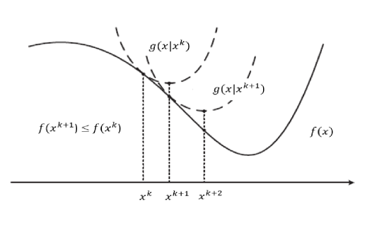
The MM procedure is depicted in Fig. 1, wherein g(𝐱|𝐱k)𝑔conditional𝐱superscript𝐱𝑘g({\mathbf{x}}|{\mathbf{x}}^{k}) is the surrogate function which majorizes f(𝐱)𝑓𝐱f({\mathbf{x}}) around 𝐱ksuperscript𝐱𝑘{\mathbf{x}}^{k} at the kthsuperscript𝑘𝑡k^{th} iteration. Pictorially, it can be seen that f(𝐱k+2)<f(𝐱k+1)<f(𝐱k)𝑓superscript𝐱𝑘2𝑓superscript𝐱𝑘1𝑓superscript𝐱𝑘f({\mathbf{x}}^{k+2})<f({\mathbf{x}}^{k+1})<f({\mathbf{x}}^{k}).

Refer to caption
Figure 1: MM procedure [29]

By using (9), (10) and (11) it can be shown mathematically that the objective function is monotonically decreased at every iteration:

f(𝐱k+1)g(𝐱k+1|𝐱k)g(𝐱k|𝐱k)=f(𝐱k)𝑓superscript𝐱𝑘1𝑔conditionalsuperscript𝐱𝑘1superscript𝐱𝑘𝑔conditionalsuperscript𝐱𝑘superscript𝐱𝑘𝑓superscript𝐱𝑘f({\mathbf{x}}^{k+1})\leq g\left({\mathbf{x}}^{k+1}|{\mathbf{x}}^{k}\right)\leq g\left({\mathbf{x}}^{k}|{\mathbf{x}}^{k}\right)=f({\mathbf{x}}^{k}) (12)

The first inequality and the last equality are by using (9) and (10), respectively. The second inequality is by (11). The convergence rate and computational complexity of the algorithm depends on how well one formulates the surrogate function. The convergence rate depends on how well the surrogate function follows the shape of the objective function f(𝐱)𝑓𝐱f({\mathbf{x}}) and to have lower computational complexity, the surrogate function must be easy to minimize. Hence, the novelty of the algorithm based on MM lies in the design of the surrogate function. Moreover, in the case of multivariate optimization problem, if the surrogate function is separable in the optimization variables - then the minimization problem could be solved parallely, which gives the computational advantage. To design surrogate function there are no set steps to follow. However, there are few papers which give guidelines for designing various surrogate functions [30], [29].

II-B Block MM

Suppose that the optimization variable 𝐱𝐱{{\mathbf{x}}} can be split into m𝑚{m} blocks as 𝐱=(𝐱1,𝐱2,,𝐱m)𝐱subscript𝐱1subscript𝐱2subscript𝐱𝑚{\mathbf{x}}=({\mathbf{x}}_{1},{\mathbf{x}}_{2},\cdots,{\mathbf{x}}_{m}), then one could apply Block MM to solve the optimization problem f(𝐱)𝑓𝐱f({\mathbf{x}}). Block MM, an extension of vanilla MM, is a combination of block coordinate descent and vanilla MM wherein the optimization variable is split into several blocks and each block is updated using vanilla MM while keeping the other blocks fixed. Hence, the ithsuperscript𝑖𝑡{i}^{th} block is updated by minimizing the surrogate function gi(𝐱i|𝐱k)subscript𝑔𝑖conditionalsubscript𝐱𝑖superscript𝐱𝑘g_{i}\left({\mathbf{x}}_{i}|{\mathbf{x}}^{k}\right) which majorizes f(𝐱)𝑓𝐱f({\mathbf{x}}) on the ithsuperscript𝑖𝑡{i}^{th} block and has to satisfy the following properties:

gi(𝐱ik|𝐱k)=f(𝐱k)subscript𝑔𝑖conditionalsubscript𝐱𝑖k𝐱k𝑓superscript𝐱𝑘g_{i}{({\mathbf{x}}_{i}\textsuperscript{k}|{\mathbf{x}}\textsuperscript{k})}=f({\mathbf{x}}^{k}) (13)
gi(𝐱i|𝐱k)f(𝐱1k,𝐱i,𝐱mk)subscript𝑔𝑖conditionalsubscript𝐱𝑖superscript𝐱𝑘𝑓superscriptsubscript𝐱1𝑘subscript𝐱𝑖superscriptsubscript𝐱𝑚𝑘g_{i}({\mathbf{x}}_{i}|{\mathbf{x}}^{k})\geq f({{\mathbf{x}}_{1}}^{k},\cdots{\mathbf{x}}_{i},\cdots{{\mathbf{x}}_{m}}^{k}) (14)

where 𝐱ksuperscript𝐱𝑘{\mathbf{x}}^{k} is the value taken by 𝐱𝐱{\mathbf{x}} at the kthsuperscript𝑘𝑡k^{th} iteration. The i𝑖{i}th block at k+1𝑘1{k+1} iteration is updated by solving the following problem:

𝐱ik+1argmin𝐱igi(𝐱i|𝐱k)superscriptsubscript𝐱𝑖𝑘1subscript𝐱𝑖argminsubscriptgiconditionalsubscript𝐱isuperscript𝐱k{{\mathbf{x}}_{i}}^{k+1}\in\underset{{\mathbf{x}}_{i}}{\rm arg\>min}\quad g_{i}\left({\mathbf{x}}_{i}|{\mathbf{x}}^{k}\right) (15)

Each block in Block MM is usually updated in a cyclic fashion. The Block MM procedure is as shown in Fig. 2.
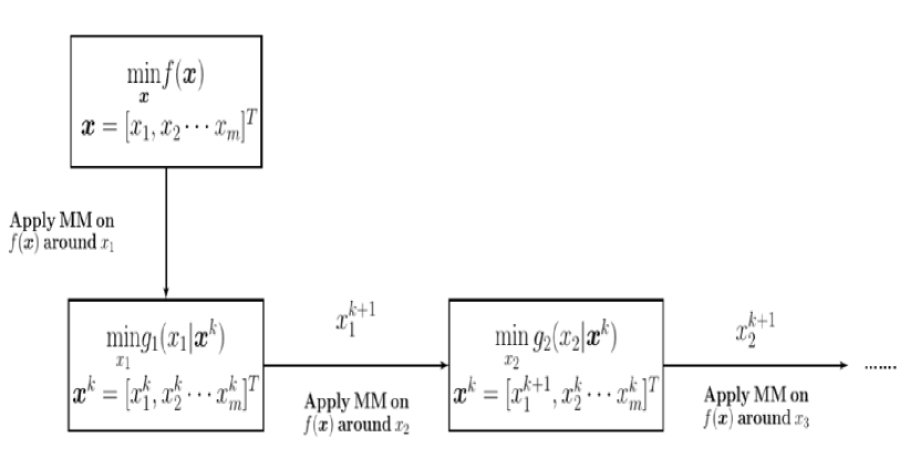
Refer to caption
Figure 2: Block MM procedure

The surrogate function for block MM must be chosen in such a way that the surrogate function is easy to minimize and must also approximate the objective function well to have faster convergence. Moreover, it is also reported that in some cases the surrogate function in case of block MM can approximate the objective function better than using a single block, leading to a faster convergence rate [29].

III Algorithms for NMF problem

In this section, we propose two iterative algorithms to solve the NMF problem in (1) based on block MM and vanilla MM. The first algorithm - INOM is based on block MM and sequentially updates both the matrices. The second algorithm - PARINOM is based on vanilla MM and parallely updates the 𝐖𝐖{\mathbf{W}} and 𝐇𝐇{\mathbf{H}} matrices. We then discuss the convergence of the two algorithms and show that they always converge to the stationary point. At the end of the section, we also show a way to accelerate the convergence of PARINOM algorithm, with a little additional computational cost.

III-A INOM:Iterative NOnnegative Matrix Factorization

This algorithm is based on Block Majorization Minimization principle wherein 𝐖𝐖{\mathbf{W}} and 𝐇𝐇{\mathbf{H}} are considered as blocks and each block is updated by vanilla MM scheme while keeping the other blocks fixed.

Before we derive the update equation for 𝐖𝐖{\mathbf{W}} and 𝐇𝐇{\mathbf{H}} matrices, we first point out an important observation that is subsequently used to form the surrogate functions g𝐖(𝐖|𝐇k,𝐖k)subscript𝑔𝐖conditional𝐖superscript𝐇𝑘superscript𝐖𝑘g_{{}_{{\mathbf{W}}}}\left({\mathbf{W}}|{\mathbf{H}}^{k},{\mathbf{W}}^{k}\right) and g𝐇(𝐇|𝐖k,𝐇k)subscript𝑔𝐇conditional𝐇superscript𝐖𝑘superscript𝐇𝑘g_{{}_{{\mathbf{H}}}}\left({\mathbf{H}}|{\mathbf{W}}^{k},{\mathbf{H}}^{k}\right), which is used to majorize the function fNMF(𝐖,𝐇)subscript𝑓NMF𝐖𝐇f_{{}_{\rm NMF}}\left({\mathbf{W}},{\mathbf{H}}\right) on the 𝐖thsuperscript𝐖𝑡{\mathbf{W}}^{th} and 𝐇thsuperscript𝐇𝑡{\mathbf{H}}^{th} block, respectively. To discuss the same, we re-write fNMF(𝐖,𝐇)subscript𝑓NMF𝐖𝐇f_{{}_{\rm NMF}}\left({\mathbf{W}},{\mathbf{H}}\right) as:

fNMF(𝐖,𝐇)=𝐕𝐖𝐇F2=j=1m𝐯j𝐖𝐡j2subscript𝑓NMF𝐖𝐇superscriptsubscriptnorm𝐕𝐖𝐇𝐹2superscriptsubscript𝑗1𝑚superscriptnormsubscript𝐯𝑗subscript𝐖𝐡𝑗2missing-subexpression\begin{array}[]{ll}f_{{}_{\rm NMF}}\left({\mathbf{W}},{\mathbf{H}}\right)=\|{\mathbf{V}}-{\mathbf{W}}{\mathbf{H}}\|_{F}^{2}=\displaystyle\sum_{j=1}^{m}\|{\mathbf{v}}_{j}-{\mathbf{W}}{\mathbf{h}}_{j}\|^{2}\end{array} (16)

where 𝐯jsubscript𝐯𝑗{\mathbf{v}}_{j} and 𝐡jsubscript𝐡𝑗{\mathbf{h}}_{j} is the jthsuperscript𝑗𝑡j^{th} column of 𝐕𝐕{\mathbf{V}} and 𝐇𝐇{\mathbf{H}}, respectively. From (16), it can be seen that given 𝐖=𝐖k𝐖superscript𝐖𝑘{\mathbf{W}}={\mathbf{W}}^{k}, the fNMF(𝐖k,𝐇)subscript𝑓NMFsuperscript𝐖𝑘𝐇f_{{}_{\rm NMF}}\left({\mathbf{W}}^{k},{\mathbf{H}}\right) is separable on each column of 𝐇𝐇{\mathbf{H}}. On taking the partial derivative of the above function with respect to 𝐡jsubscript𝐡𝑗{{\mathbf{h}}_{j}}, we get

fNMF(𝐡j|𝐖k)=2(𝐖k)T𝐯j+2(𝐖k)T𝐖k𝐡j2fNMF(𝐡j|𝐖k)=2(𝐖k)T𝐖ksubscript𝑓NMFconditionalsubscript𝐡𝑗superscript𝐖𝑘2superscriptsuperscript𝐖𝑘𝑇subscript𝐯𝑗2superscriptsuperscript𝐖𝑘𝑇superscript𝐖𝑘subscript𝐡𝑗missing-subexpressionmissing-subexpressionmissing-subexpressionsuperscript2subscript𝑓NMFconditionalsubscript𝐡𝑗superscript𝐖𝑘2superscriptsuperscript𝐖𝑘𝑇superscript𝐖𝑘missing-subexpression\begin{array}[]{ll}\nabla f_{{}_{\rm NMF}}({\mathbf{h}}_{j}|{\mathbf{W}}^{k})=-2({\mathbf{W}}^{k})^{T}{\mathbf{v}}_{j}+2({\mathbf{W}}^{k})^{T}{\mathbf{W}}^{k}{\mathbf{h}}_{j}\\ \\ \nabla^{2}f_{{}_{\rm NMF}}({\mathbf{h}}_{j}|{\mathbf{W}}^{k})=2({\mathbf{W}}^{k})^{T}{\mathbf{W}}^{k}\end{array} (17)

Note that the Hessian matrix 2(𝐖k)T𝐖k2superscriptsuperscript𝐖𝑘𝑇superscript𝐖𝑘2({\mathbf{W}}^{k})^{T}{\mathbf{W}}^{k} consists only of nonnegative entries and is independent of 𝐡jsubscript𝐡𝑗{\mathbf{h}}_{j}. We now show that fNMF(𝐖,𝐇k)subscript𝑓NMF𝐖superscript𝐇𝑘f_{{}_{\rm NMF}}\left({\mathbf{W}},{\mathbf{H}}^{k}\right) is separable on each row of 𝐖𝐖{\mathbf{W}} and the Hessian of fNMF(𝐖,𝐇k)subscript𝑓NMF𝐖superscript𝐇𝑘f_{{}_{\rm NMF}}\left({\mathbf{W}},{\mathbf{H}}^{k}\right) with respect to jthsuperscript𝑗𝑡j^{th} row of 𝐖𝐖{\mathbf{W}} is nonnegative and is equal to 2𝐇k(𝐇k)T2superscript𝐇𝑘superscriptsuperscript𝐇𝑘𝑇2{\mathbf{H}}^{k}({\mathbf{H}}^{k})^{T}:

fNMF(𝐖,𝐇k)=𝐕𝐖𝐇kF2=j=1n𝐯j𝐰j𝐇kF2subscript𝑓NMF𝐖superscript𝐇𝑘superscriptsubscriptnorm𝐕superscript𝐖𝐇𝑘𝐹2superscriptsubscript𝑗1𝑛superscriptsubscriptnormsubscriptsuperscript𝐯𝑗subscript𝐰𝑗superscript𝐇𝑘𝐹2missing-subexpression\begin{array}[]{ll}f_{{}_{\rm NMF}}\left({\mathbf{W}},{\mathbf{H}}^{k}\right)=\|{\mathbf{V}}-{\mathbf{W}}{\mathbf{H}}^{k}\|_{F}^{2}=\displaystyle\sum_{j=1}^{n}\|{\mathbf{v}}^{\prime}_{j}-{\mathbf{w}}_{j}{\mathbf{H}}^{k}\|_{F}^{2}\end{array} (18)

where 𝐯jsubscriptsuperscript𝐯𝑗{\mathbf{v}}^{\prime}_{j} and 𝐰jsubscript𝐰𝑗{\mathbf{w}}_{j} represent the jthsuperscript𝑗𝑡{j^{th}} row of 𝐕𝐕{\mathbf{V}} and 𝐖𝐖{\mathbf{W}}, respectively.

fNMF(𝐰j|𝐇k)=2𝐯j𝐇kT+2𝐰j𝐇k𝐇kT2fNMF(𝐰j|𝐇k)=2𝐇k𝐇kTsubscript𝑓NMFconditionalsubscript𝐰𝑗superscript𝐇𝑘2subscriptsuperscript𝐯𝑗superscriptsuperscript𝐇𝑘𝑇2subscript𝐰𝑗superscript𝐇𝑘superscriptsuperscript𝐇𝑘𝑇missing-subexpressionmissing-subexpressionmissing-subexpressionsuperscript2subscript𝑓NMFconditionalsubscript𝐰𝑗superscript𝐇𝑘2superscript𝐇𝑘superscriptsuperscript𝐇𝑘𝑇missing-subexpression\begin{array}[]{ll}\nabla f_{{}_{\rm NMF}}({\mathbf{w}}_{j}|{\mathbf{H}}^{k})=-2{\mathbf{v}}^{\prime}_{j}{{{\mathbf{H}}^{k}}}^{T}+2{\mathbf{w}}_{j}{\mathbf{H}}^{k}{{\mathbf{H}}^{k}}^{T}\\ \\ \nabla^{2}f_{{}_{\rm NMF}}({\mathbf{w}}_{j}|{\mathbf{H}}^{k})=2{\mathbf{H}}^{k}{{\mathbf{H}}^{k}}^{T}\end{array} (19)

We smartly use the nonnegative Hessian matrix to design the upper bounds g𝐖(𝐖|𝐇k,𝐖k)subscript𝑔𝐖conditional𝐖superscript𝐇𝑘superscript𝐖𝑘g_{{}_{{\mathbf{W}}}}\left({\mathbf{W}}|{\mathbf{H}}^{k},{\mathbf{W}}^{k}\right) and g𝐇(𝐇|𝐖k,𝐇k)subscript𝑔𝐇conditional𝐇superscript𝐖𝑘superscript𝐇𝑘g_{{}_{{\mathbf{H}}}}\left({\mathbf{H}}|{\mathbf{W}}^{k},{\mathbf{H}}^{k}\right), based on the following lemmas.

Lemma III.1

Lower Quadratic Bound Principle [30], [31]: Given 𝐱=𝐱k𝐱superscript𝐱𝑘{\mathbf{x}}={\mathbf{x}}^{k}, a twice differentiable function f(𝐱)𝑓𝐱f({\mathbf{x}}), a square matrix ΛΛ\Lambda such that Λ2f(𝐱)succeeds-or-equalsΛsuperscript2𝑓𝐱\Lambda\succcurlyeq\nabla^{2}f({\mathbf{x}}), then f(𝐱)𝑓𝐱f({\mathbf{x}}) can be upper bounded as

f(𝐱)f(𝐱k)+f(𝐱k)T(𝐱𝐱k)+12(𝐱𝐱k)TΛ(𝐱𝐱k)𝑓𝐱𝑓superscript𝐱𝑘𝑓superscriptsuperscript𝐱𝑘𝑇𝐱superscript𝐱𝑘12superscript𝐱superscript𝐱𝑘𝑇Λ𝐱superscript𝐱𝑘missing-subexpression\begin{array}[]{ll}f({\mathbf{x}})\leq f({\mathbf{x}}^{k})+\nabla f({\mathbf{x}}^{k})^{T}({\mathbf{x}}-{\mathbf{x}}^{k})+\dfrac{1}{2}({\mathbf{x}}-{\mathbf{x}}^{k})^{T}\Lambda({\mathbf{x}}-{\mathbf{x}}^{k})\end{array} (20)

The upper bound for f(𝐱)𝑓𝐱f({\mathbf{x}}) is quadratic and differentiable in 𝐱𝐱{\mathbf{x}}.

Proof:

Suppose there exists a matrix ΛΛ\Lambda, such that Λ2f(𝐱)succeeds-or-equalsΛsuperscript2𝑓𝐱\Lambda\succcurlyeq\nabla^{2}f({\mathbf{x}}), then we have the following equality by second order Taylor expansion:

f(𝐱)f(𝐱k)+f(𝐱k)T(𝐱𝐱k)+12(𝐱𝐱k)TΛ(𝐱𝐱k)𝑓𝐱𝑓superscript𝐱𝑘𝑓superscriptsuperscript𝐱𝑘𝑇𝐱superscript𝐱𝑘12superscript𝐱superscript𝐱𝑘𝑇Λ𝐱superscript𝐱𝑘f({\mathbf{x}})\leq f({\mathbf{x}}^{k})+\nabla f({\mathbf{x}}^{k})^{T}({\mathbf{x}}-{\mathbf{x}}^{k})+\dfrac{1}{2}({\mathbf{x}}-{\mathbf{x}}^{k})^{T}\Lambda({\mathbf{x}}-{\mathbf{x}}^{k})

and equality is achieved at 𝐱=𝐱k𝐱superscript𝐱𝑘{\mathbf{x}}={\mathbf{x}}^{k}. ∎

Lemma III.2

Let 𝐀𝐀{{\mathbf{A}}} of size n×n𝑛𝑛n\times n denote a nonnegative, square and symmetric matrix and let p𝑝p \in 𝐑+superscript𝐑\mathbf{R^{+}}. We define ΛΛ\Lambda as a diagonal matrix with its diagonal elements equal to p𝑝p, the maximum row sum of 𝐀𝐀{{\mathbf{A}}} matrix. Then, Λ𝐀succeeds-or-equalsΛ𝐀\Lambda\succcurlyeq{{\mathbf{A}}}.

Proof:

The above lemma is based on Perron-Frobenius Theorem [32], [33]. According to the theorem, there is a positive real number p𝑝p, called the Perron root, such that any other eigenvalue λ𝜆\lambda of 𝐀𝐀{\mathbf{A}} in absolute value is strictly smaller than p𝑝p i.e. |λ|<p𝜆𝑝|\lambda|<p. To calculate p𝑝p, an important corollary of the theorem is used:

pmax𝑖j=1naij𝑝𝑖maxsuperscriptsubscriptj1nsubscriptaijmissing-subexpression\begin{array}[]{ll}p\leq\underset{i}{\rm max}\displaystyle\sum_{j=1}^{n}a_{ij}\end{array} (21)

where aijsubscript𝑎𝑖𝑗a_{ij} is the (i,j)thsuperscript𝑖𝑗𝑡(i,j)^{th} element of 𝐀𝐀{\mathbf{A}} matrix. Hence, we get the following inequality:

max𝑖j=1naijp>λ𝑖maxsuperscriptsubscriptj1nsubscriptaijp𝜆\underset{i}{\rm max}\displaystyle\sum_{j=1}^{n}a_{ij}\geq p>\lambda (22)

By constructing a diagonal matrix ΛΛ\Lambda with its diagonal elements as maximum row sum of 𝐀𝐀{\mathbf{A}} and by using Eigen Value Decomposition, the inequality Λ𝐀succeeds-or-equalsΛ𝐀\Lambda\succcurlyeq{{\mathbf{A}}} is attained.

Using lemma III.1 and lemma III.2, we construct the surrogate function g𝐇(𝐇|𝐇k,𝐖k)subscript𝑔𝐇conditional𝐇superscript𝐇𝑘superscript𝐖𝑘g_{{}_{\mathbf{H}}}\left({\mathbf{H}}|{\mathbf{H}}^{k},{\mathbf{W}}^{k}\right) for the problem in (16) to update the 𝐇thsuperscript𝐇𝑡{\mathbf{H}}^{th} block with 𝐖ksuperscript𝐖𝑘{\mathbf{W}}^{k} fixed.

g𝐇(𝐇|𝐇k,𝐖k)=j=1mg𝐡j(𝐡j|𝐡jk,𝐖k)=j=1mf(𝐡jk)+f(𝐡jk)T(𝐡j𝐡jk)+12(𝐡j𝐡jk)TΛk(𝐡j𝐡jk)subscript𝑔𝐇conditional𝐇superscript𝐇𝑘superscript𝐖𝑘superscriptsubscript𝑗1𝑚subscript𝑔subscript𝐡𝑗conditionalsubscript𝐡𝑗superscriptsubscript𝐡𝑗𝑘superscript𝐖𝑘superscriptsubscript𝑗1𝑚𝑓superscriptsubscript𝐡𝑗𝑘𝑓superscriptsuperscriptsubscript𝐡𝑗𝑘𝑇subscript𝐡𝑗superscriptsubscript𝐡𝑗𝑘12superscriptsubscript𝐡𝑗superscriptsubscript𝐡𝑗𝑘𝑇superscriptΛ𝑘subscript𝐡𝑗superscriptsubscript𝐡𝑗𝑘missing-subexpression\begin{array}[]{ll}g_{{}_{\mathbf{H}}}\left({\mathbf{H}}|{\mathbf{H}}^{k},{\mathbf{W}}^{k}\right)=\displaystyle\sum_{j=1}^{m}g_{{\mathbf{h}}_{j}}\left({{\mathbf{h}}_{j}}|{{\mathbf{h}}_{j}}^{k},{\mathbf{W}}^{k}\right)=\displaystyle\sum_{j=1}^{m}f({\mathbf{h}}_{j}^{k})+\nabla f({\mathbf{h}}_{j}^{k})^{T}({\mathbf{h}}_{j}-{\mathbf{h}}_{j}^{k})+\dfrac{1}{2}({\mathbf{h}}_{j}-{\mathbf{h}}_{j}^{k})^{T}\Lambda^{k}({\mathbf{h}}_{j}-{\mathbf{h}}_{j}^{k})\end{array} (23)

where ΛksuperscriptΛ𝑘\Lambda^{k} matrix is a diagonal matrix with its diagonal elements as maximum row sum of 2(𝐖k)T𝐖k2superscriptsuperscript𝐖𝑘𝑇superscript𝐖𝑘{2{({\mathbf{W}}^{k})}^{T}{{\mathbf{W}}^{k}}} and f(𝐡jk)𝑓superscriptsubscript𝐡𝑗𝑘\nabla f({\mathbf{h}}_{j}^{k}) is equal to 2(𝐖k)T𝐯j+2(𝐖k)T𝐖k𝐡jk2superscriptsuperscript𝐖𝑘𝑇subscript𝐯𝑗2superscriptsuperscript𝐖𝑘𝑇superscript𝐖𝑘superscriptsubscript𝐡𝑗𝑘-2{({\mathbf{W}}^{k})}^{T}{\mathbf{v}}_{j}+2{({\mathbf{W}}^{k})}^{T}{\mathbf{W}}^{k}{{\mathbf{h}}_{j}}^{k}. The surrogate function is separable in each column of 𝐇𝐇{\mathbf{H}}. Hence at any iteration, given 𝐖=𝐖k𝐖superscript𝐖𝑘{\mathbf{W}}={\mathbf{W}}^{k} and 𝐇=𝐇k𝐇superscript𝐇𝑘{\mathbf{H}}={\mathbf{H}}^{k}, the surrogate minimization problem is:

minimize𝐇0g𝐇(𝐇|𝐇k,𝐖k)𝐇0minimizesubscriptg𝐇conditional𝐇superscript𝐇ksuperscript𝐖kmissing-subexpression\begin{array}[]{ll}\underset{{\mathbf{H}}\geq 0}{\rm minimize}\>g_{{}_{\mathbf{H}}}\left({\mathbf{H}}|{\mathbf{H}}^{k},{\mathbf{W}}^{k}\right)\end{array} (24)

which has a closed form solution given by:

𝐡jk+1=𝐡jk+1μk(2(𝐖k)T𝐯j2(𝐖k)T𝐖k𝐡jk)𝐡jk+1=𝐡jk+1μk((2(𝐖k)T𝐕)j(2(𝐖k)T𝐖k𝐇k)j)superscriptsubscript𝐡𝑗𝑘1superscriptsubscript𝐡𝑗𝑘1superscript𝜇𝑘2superscriptsuperscript𝐖𝑘𝑇subscript𝐯𝑗2superscriptsuperscript𝐖𝑘𝑇superscript𝐖𝑘superscriptsubscript𝐡𝑗𝑘missing-subexpressionmissing-subexpressionmissing-subexpressionsuperscriptsubscript𝐡𝑗𝑘1superscriptsubscript𝐡𝑗𝑘1superscript𝜇𝑘subscript2superscriptsuperscript𝐖𝑘𝑇𝐕𝑗subscript2superscriptsuperscript𝐖𝑘𝑇superscript𝐖𝑘superscript𝐇𝑘𝑗missing-subexpression\begin{array}[]{ll}{\mathbf{h}}_{j}^{k+1}={\mathbf{h}}_{j}^{k}+\dfrac{1}{\mu^{k}}\left({2{{\left({\mathbf{W}}^{k}\right)}^{T}}{{\mathbf{v}}_{j}}-{2{{\left({\mathbf{W}}^{k}\right)}^{T}}{{\mathbf{W}}^{k}}{\mathbf{h}}_{j}^{k}}}\right)\\ \\ {\mathbf{h}}_{j}^{k+1}={\mathbf{h}}_{j}^{k}+\dfrac{1}{\mu^{k}}\left({\left(2{{\left({\mathbf{W}}^{k}\right)}^{T}}{\mathbf{V}}\right)_{j}}-{\left(2{\left({\mathbf{W}}^{k}\right)}^{T}{\mathbf{W}}^{k}{\mathbf{H}}^{k}\right)_{j}}\right)\end{array} (25)

where μksuperscript𝜇𝑘\mu^{k} = maximum row sum of 2(𝐖k)T𝐖k2superscriptsuperscript𝐖𝑘𝑇superscript𝐖𝑘{2{({\mathbf{W}}^{k})}^{T}{{\mathbf{W}}^{k}}}. Since the update of jthsuperscript𝑗𝑡j^{th} column of 𝐇𝐇{\mathbf{H}} does not depend on the update of (j+1)thsuperscript𝑗1𝑡({j+1})^{th} column of 𝐇𝐇{\mathbf{H}}, we can re-write the above update equation as:

𝐇k+1=𝐇k+1μk(2(𝐖k)T𝐕2(𝐖k)T𝐖k𝐇k)superscript𝐇𝑘1superscript𝐇𝑘1superscript𝜇𝑘2superscriptsuperscript𝐖𝑘𝑇𝐕2superscriptsuperscript𝐖𝑘𝑇superscript𝐖𝑘superscript𝐇𝑘missing-subexpression\begin{array}[]{ll}{\mathbf{H}}^{k+1}={\mathbf{H}}^{k}+\dfrac{1}{\mu^{k}}\left(2{\left({\mathbf{W}}^{k}\right)}^{T}{\mathbf{V}}-2{\left({\mathbf{W}}^{k}\right)}^{T}{{\mathbf{W}}^{k}}{\mathbf{H}}^{k}\right)\end{array} (26)

We now construct the surrogate function g𝐖(𝐖|𝐖k,𝐇k+1)subscript𝑔𝐖conditional𝐖superscript𝐖𝑘superscript𝐇𝑘1g_{{}_{\mathbf{W}}}\left({\mathbf{W}}|{\mathbf{W}}^{k},{\mathbf{H}}^{k+1}\right) using lemma III.1 and lemma III.2 for the problem in (18) to update the 𝐖thsuperscript𝐖𝑡{\mathbf{W}}^{th} block with 𝐇k+1superscript𝐇𝑘1{\mathbf{H}}^{k+1} fixed.

g𝐖(𝐖|𝐖k,𝐇k+1)=j=1ng𝐰j(𝐰j|𝐰jk,𝐇k)=j=1nf(𝐰jk)+(𝐰j𝐰jk)f(𝐰jk)T+12(𝐰j𝐰jk)Λk(𝐰j𝐰jk)Tsubscript𝑔𝐖conditional𝐖superscript𝐖𝑘superscript𝐇𝑘1superscriptsubscript𝑗1𝑛subscript𝑔subscript𝐰𝑗conditionalsubscript𝐰𝑗superscriptsubscript𝐰𝑗𝑘superscript𝐇𝑘superscriptsubscript𝑗1𝑛𝑓superscriptsubscript𝐰𝑗𝑘subscript𝐰𝑗superscriptsubscript𝐰𝑗𝑘𝑓superscriptsuperscriptsubscript𝐰𝑗𝑘𝑇12subscript𝐰𝑗superscriptsubscript𝐰𝑗𝑘superscriptΛ𝑘superscriptsubscript𝐰𝑗superscriptsubscript𝐰𝑗𝑘𝑇missing-subexpression\begin{array}[]{ll}g_{{}_{\mathbf{W}}}\left({\mathbf{W}}|{\mathbf{W}}^{k},{\mathbf{H}}^{k+1}\right)=\displaystyle\sum_{j=1}^{n}g_{{\mathbf{w}}_{j}}\left({{\mathbf{w}}_{j}}|{{\mathbf{w}}_{j}}^{k},{\mathbf{H}}^{k}\right)=\displaystyle\sum_{j=1}^{n}f({\mathbf{w}}_{j}^{k})+({\mathbf{w}}_{j}-{\mathbf{w}}_{j}^{k})\nabla f({\mathbf{w}}_{j}^{k})^{T}+\dfrac{1}{2}({\mathbf{w}}_{j}-{\mathbf{w}}_{j}^{k})\Lambda^{k}({\mathbf{w}}_{j}-{\mathbf{w}}_{j}^{k})^{T}\end{array} (27)

where ΛksuperscriptΛ𝑘{\Lambda^{k}} matrix is constructed with its diagonal elements as maximum row sum of 2(𝐇k+1)(𝐇k+1)T2superscript𝐇𝑘1superscriptsuperscript𝐇𝑘1𝑇{2({\mathbf{H}}^{k+1})({{\mathbf{H}}^{k+1}})^{T}} and f(𝐰jk)=2𝐯j(𝐇k+1)T+2𝐰j(𝐇k+1)(𝐇k+1)T𝑓superscriptsubscript𝐰𝑗𝑘2subscriptsuperscript𝐯𝑗superscriptsuperscript𝐇𝑘1𝑇2subscript𝐰𝑗superscript𝐇𝑘1superscriptsuperscript𝐇𝑘1𝑇\nabla f({\mathbf{w}}_{j}^{k})=-2{\mathbf{v}}^{\prime}_{j}({{{\mathbf{H}}}^{k+1}})^{T}+2{\mathbf{w}}_{j}({\mathbf{H}}^{k+1})({{\mathbf{H}}^{k+1}})^{T}. The surrogate function is separable in each row of 𝐖𝐖{\mathbf{W}}. Hence at any iteration, given 𝐖=𝐖k𝐖superscript𝐖𝑘{\mathbf{W}}={\mathbf{W}}^{k} and 𝐇=𝐇k+1𝐇superscript𝐇𝑘1{\mathbf{H}}={\mathbf{H}}^{k+1}, the surrogate minimization problem is:

minimize𝐖0g𝐖(𝐖|𝐖k,𝐇k+1)𝐖0minimizesubscriptg𝐖conditional𝐖superscript𝐖ksuperscript𝐇k1missing-subexpression\begin{array}[]{ll}\underset{{\mathbf{W}}\geq 0}{\rm minimize}\>g_{{}_{\mathbf{W}}}\left({\mathbf{W}}|{\mathbf{W}}^{k},{\mathbf{H}}^{k+1}\right)\end{array} (28)

which has a closed form solution given by:

𝐖k+1=𝐖k+1νk(2𝐕𝐇k+1T2𝐖k𝐇k+1𝐇k+1T)superscript𝐖𝑘1superscript𝐖𝑘1superscript𝜈𝑘2superscriptsuperscript𝐕𝐇𝑘1𝑇2superscript𝐖𝑘superscript𝐇𝑘1superscriptsuperscript𝐇𝑘1𝑇missing-subexpression\begin{array}[]{ll}{\mathbf{W}}^{k+1}={\mathbf{W}}^{k}+\dfrac{1}{\nu^{k}}\left(2{\mathbf{V}}{{\mathbf{H}}^{k+1}}^{T}-2{\mathbf{W}}^{k}{\mathbf{H}}^{k+1}{{\mathbf{H}}^{k+1}}^{T}\right)\end{array} (29)

where νksuperscript𝜈𝑘\nu^{k} = maximum row sum of 2𝐇k+1𝐇k+1T2superscript𝐇𝑘1superscriptsuperscript𝐇𝑘1𝑇{2{\mathbf{H}}^{k+1}{{\mathbf{H}}^{k+1}}^{T}}. Note that once 𝐇k+1superscript𝐇𝑘1{\mathbf{H}}^{k+1} and 𝐖k+1superscript𝐖𝑘1{\mathbf{W}}^{k+1} are computed using (26) and (29), the negative elements must be projected back to 𝐑+superscript𝐑\mathbf{R^{+}}, to satisfy the nonnegative constraint. Also, observe that the update equations looks similar to gradient descent algorithm with “adaptive” step sizes equal to μksuperscript𝜇𝑘\mu^{k} and νksuperscript𝜈𝑘\nu^{k}. Typically, line search algorithm is implemented to iteratively search for the optimal step sizes until the objective function decreases [34]. Nevertheless, we don’t have to iteratively search for the optimal step sizes; since the proposed algorithm is based on block MM-it is guaranteed that the step sizes - νksuperscript𝜈𝑘\nu^{k} and μksuperscript𝜇𝑘\mu^{k} will ensure the monotonic decrease of the respective cost functions. We now calculate the computational complexity of INOM algorithm. The complexity of computing μksuperscript𝜇𝑘\mu^{k} and νksuperscript𝜈𝑘\nu^{k} is 𝒪(r2n)𝒪superscript𝑟2𝑛\mathcal{O}(r^{2}n) and 𝒪(r2m)𝒪superscript𝑟2𝑚\mathcal{O}(r^{2}m), respectively. The complexity of computing 𝐇k+1superscript𝐇𝑘1{\mathbf{H}}^{k+1} is 𝒪(rnm)+𝒪(r2(n+m))𝒪𝑟𝑛𝑚𝒪superscript𝑟2𝑛𝑚\mathcal{O}(rnm)+\mathcal{O}(r^{2}(n+m)). The complexity of computing 𝐖k+1superscript𝐖𝑘1{\mathbf{W}}^{k+1} is 𝒪(rnm)+𝒪(r2(n+m))𝒪𝑟𝑛𝑚𝒪superscript𝑟2𝑛𝑚\mathcal{O}(rnm)+\mathcal{O}(r^{2}(n+m)). Since INOM is a sequential algorithm, the total complexity of the algorithm is 𝒪(2rnm+2r2(n+m))𝒪2𝑟𝑛𝑚2superscript𝑟2𝑛𝑚\mathcal{O}(2rnm+2r^{2}(n+m)). Pseudo code of INOM is shown in Table 2.

Table 2: INOM
Input: Data samples 𝐕𝐕{{\mathbf{V}}} with each column normalized; r𝑟{r}, m𝑚{m} and n𝑛{n}.
Initialize: Set k𝑘{k} = 0. Initialize 𝐖0superscript𝐖0{{\mathbf{W}}^{0}} and 𝐇0superscript𝐇0{{\mathbf{H}}^{0}}. Each column of 𝐖0superscript𝐖0{{\mathbf{W}}^{0}} is normalized.
Repeat:
Update 𝐇𝐇{{\mathbf{H}}}
1) μksuperscript𝜇𝑘\mu^{k} = maximum row sum of 2𝐖kT𝐖k2superscriptsuperscript𝐖𝑘𝑇superscript𝐖𝑘{2{{\mathbf{W}}^{k}}^{T}{{\mathbf{W}}^{k}}}
2) 𝐇k+1=𝐇k+1μk(2𝐖kT𝐕2𝐖kT𝐖k𝐇k)superscript𝐇𝑘1superscript𝐇𝑘1superscript𝜇𝑘2superscriptsuperscript𝐖𝑘𝑇𝐕2superscriptsuperscript𝐖𝑘𝑇superscript𝐖𝑘superscript𝐇𝑘{\mathbf{H}}^{k+1}={\mathbf{H}}^{k}+\dfrac{1}{\mu^{k}}\left(2{{\mathbf{W}}^{k}}^{T}{\mathbf{V}}-2{{\mathbf{W}}^{k}}^{T}{{\mathbf{W}}^{k}}{\mathbf{H}}^{k}\right)
3) 𝐇k+1=max(𝟎,𝐇𝐤+𝟏)superscript𝐇𝑘1max0superscript𝐇𝐤1{\mathbf{H}}^{k+1}=\textrm{max}(\bf{\bf{0}},{\mathbf{H}}^{k+1})
Update 𝐖𝐖{{\mathbf{W}}}
4) νksuperscript𝜈𝑘\nu^{k} = maximum row sum of 2𝐇k+1𝐇k+1T2superscript𝐇𝑘1superscriptsuperscript𝐇𝑘1𝑇{2{\mathbf{H}}^{k+1}{{\mathbf{H}}^{k+1}}^{T}}
5) 𝐖k+1=𝐖k+1νk(2𝐕𝐇k+1T2𝐖k𝐇k+1𝐇k+1T)superscript𝐖𝑘1superscript𝐖𝑘1superscript𝜈𝑘2superscriptsuperscript𝐕𝐇𝑘1𝑇2superscript𝐖𝑘superscript𝐇𝑘1superscriptsuperscript𝐇𝑘1𝑇{\mathbf{W}}^{k+1}={\mathbf{W}}^{k}+\dfrac{1}{\nu^{k}}\left(2{\mathbf{V}}{{\mathbf{H}}^{k+1}}^{T}-2{\mathbf{W}}^{k}{\mathbf{H}}^{k+1}{{\mathbf{H}}^{k+1}}^{T}\right)
6) 𝐖k+1=max(𝟎,𝐖k+1)superscript𝐖𝑘1max0superscript𝐖𝑘1{\mathbf{W}}^{k+1}=\textrm{max}({\bf{0}},{\mathbf{W}}^{k+1})
7) normalize each column of 𝐖𝐖{{\mathbf{W}}}
kk+1𝑘𝑘1k\leftarrow k+1, until |fNMF(𝐖k+1,𝐇k+1)fNMF(𝐖k,𝐇k)fNMF(𝐖k,𝐇k)|106subscript𝑓NMFsuperscript𝐖𝑘1superscript𝐇𝑘1subscript𝑓NMFsuperscript𝐖𝑘superscript𝐇𝑘subscript𝑓NMFsuperscript𝐖𝑘superscript𝐇𝑘superscript106\left|\dfrac{f_{{}_{\rm NMF}}\left({\mathbf{W}}^{k+1},{\mathbf{H}}^{k+1}\right)-f_{{}_{\rm NMF}}\left({\mathbf{W}}^{k},{\mathbf{H}}^{k}\right)}{f_{{}_{\rm NMF}}\left({\mathbf{W}}^{k},{\mathbf{H}}^{k}\right)}\right|\leq 10^{-6}

III-B PARINOM:Parallel Iterative Nonnegative Matrix Factorization

PARINOM solves the problem in (1) using Vanilla MM without alternatingly minimizing over 𝐖𝐖{\mathbf{W}} and 𝐇𝐇{\mathbf{H}} and hence at iteration i+1𝑖1i+1, 𝐇i+1superscript𝐇𝑖1{\mathbf{H}}^{i+1} matrix does not depend on 𝐖i+1superscript𝐖𝑖1{\mathbf{W}}^{i+1} matrix. Therefore, 𝐇i+1superscript𝐇𝑖1{\mathbf{H}}^{i+1} and 𝐖i+1superscript𝐖𝑖1{\mathbf{W}}^{i+1} matrix can be parallely updated. On expanding fNMF(𝐖,𝐇)subscript𝑓NMF𝐖𝐇f_{{}_{\textrm{NMF}}}\left({\mathbf{W}},{\mathbf{H}}\right) we get:

𝐕𝐖𝐇F2=Tr(𝐕T𝐕)+Tr(𝐇T𝐖T𝐖𝐇)2Tr(𝐕T𝐖𝐇)superscriptsubscriptnorm𝐕𝐖𝐇𝐹2Trsuperscript𝐕𝑇𝐕Trsuperscript𝐇𝑇superscript𝐖𝑇𝐖𝐇2Trsuperscript𝐕𝑇𝐖𝐇missing-subexpression\begin{array}[]{ll}\|{\mathbf{V}}-{\mathbf{W}}{\mathbf{H}}\|_{F}^{2}={\rm Tr}({\mathbf{V}}^{T}{\mathbf{V}})+{\rm Tr}({\mathbf{H}}^{T}{\mathbf{W}}^{T}{\mathbf{W}}{\mathbf{H}})-2{\rm Tr}({\mathbf{V}}^{T}{\mathbf{W}}{\mathbf{H}})\end{array} (30)

Ignoring the constant terms in (30), we will now show that the second and third term are sigmoidal functions, which is defined as:
Sigmoidal function [35], [36]: Let c𝑐c be a positive or a negative number and x1,x2xnsubscript𝑥1subscript𝑥2subscript𝑥𝑛{x_{1},x_{2}\cdots x_{n}} be the nonnegative components of a n𝑛n-dimensional vector 𝐱𝐱{{\mathbf{x}}}. Let αjsubscript𝛼𝑗{\alpha_{j}} be the jthsuperscript𝑗𝑡{j^{th}} component of 𝜶𝜶{\alpha}, which is the fractional power (can be positive, negative or zero) of each component of 𝐱𝐱{{\mathbf{x}}}. Then, cj=1nxjαj𝑐superscriptsubscriptproduct𝑗1𝑛superscriptsubscript𝑥𝑗subscript𝛼𝑗c\displaystyle\prod_{j=1}^{n}x_{j}^{\alpha_{j}} is called a sigmoidal function.
The second term can be re-written as:

k=1mj=1n(l=1rm=1rwjlhlkwjmhmk)superscriptsubscript𝑘1𝑚superscriptsubscript𝑗1𝑛superscriptsubscript𝑙1𝑟superscriptsubscript𝑚1𝑟subscript𝑤𝑗𝑙subscript𝑙𝑘subscript𝑤𝑗𝑚subscript𝑚𝑘missing-subexpression\begin{array}[]{ll}\displaystyle\sum_{k=1}^{m}\sum_{j=1}^{n}\left(\sum_{l=1}^{r}\sum_{m=1}^{r}w_{jl}h_{lk}w_{jm}h_{mk}\right)\end{array} (31)

where wabsubscript𝑤𝑎𝑏w_{ab} and habsubscript𝑎𝑏h_{ab} represent the (a,b)thsuperscript𝑎𝑏𝑡(a,b)^{th} element of 𝐖𝐖{\mathbf{W}} and 𝐇𝐇{\mathbf{H}} matrix. The terms in (31) are sigmoidal functions with positive coefficient. Now, we show that the third term in (30) can also be written as sigmoidal function.

2Tr(𝐕T𝐖𝐇)=2j=1nk=1m(vjkl=1rwjlhlk)2Trsuperscript𝐕𝑇𝐖𝐇2superscriptsubscript𝑗1𝑛superscriptsubscript𝑘1𝑚subscript𝑣𝑗𝑘superscriptsubscript𝑙1𝑟subscript𝑤𝑗𝑙subscript𝑙𝑘missing-subexpression\begin{array}[]{ll}-2{\rm Tr}({\mathbf{V}}^{T}{\mathbf{W}}{\mathbf{H}})=-2\displaystyle\sum_{j=1}^{n}\displaystyle\sum_{k=1}^{m}\left(v_{jk}\displaystyle\sum_{l=1}^{r}w_{jl}h_{lk}\right)\end{array} (32)

This is a sigmoidal function with negative coefficient. Hence, the objective function fNMF(𝐖,𝐇)subscript𝑓NMF𝐖𝐇f_{{}_{\textrm{NMF}}}\left({\mathbf{W}},{\mathbf{H}}\right) becomes:

𝐕𝐖𝐇F2=k=1mj=1n(l=1rm=1rwjlhlkwjmhmk)2j=1nk=1m(vjkl=1rwjlhlk)superscriptsubscriptnorm𝐕𝐖𝐇𝐹2superscriptsubscript𝑘1𝑚superscriptsubscript𝑗1𝑛superscriptsubscript𝑙1𝑟superscriptsubscript𝑚1𝑟subscript𝑤𝑗𝑙subscript𝑙𝑘subscript𝑤𝑗𝑚subscript𝑚𝑘2superscriptsubscript𝑗1𝑛superscriptsubscript𝑘1𝑚subscript𝑣𝑗𝑘superscriptsubscript𝑙1𝑟subscript𝑤𝑗𝑙subscript𝑙𝑘missing-subexpression\begin{array}[]{ll}\|{\mathbf{V}}-{\mathbf{W}}{\mathbf{H}}\|_{F}^{2}=\displaystyle\sum_{k=1}^{m}\sum_{j=1}^{n}\left(\sum_{l=1}^{r}\sum_{m=1}^{r}w_{jl}h_{lk}w_{jm}h_{mk}\right)-2\displaystyle\sum_{j=1}^{n}\displaystyle\sum_{k=1}^{m}\left(v_{jk}\displaystyle\sum_{l=1}^{r}w_{jl}h_{lk}\right)\end{array} (33)

Now, we propose the following lemma which is used to majorize the above objective function.

Lemma III.3

When c in cj=1nxjαj𝑐superscriptsubscriptproduct𝑗1𝑛superscriptsubscript𝑥𝑗subscript𝛼𝑗c\displaystyle\prod_{j=1}^{n}x_{j}^{\alpha_{j}} is positive, the following inequality holds:

cj=1nxjαjcj=1n(xji)αjj=1nαjα1(xjxji)α1csuperscriptsubscriptproduct𝑗1𝑛superscriptsubscript𝑥𝑗subscript𝛼𝑗csuperscriptsubscriptproduct𝑗1𝑛superscriptsuperscriptsubscript𝑥𝑗𝑖subscript𝛼𝑗superscriptsubscript𝑗1𝑛subscript𝛼𝑗subscriptnorm𝛼1superscriptsubscript𝑥𝑗superscriptsubscript𝑥𝑗𝑖subscriptnorm𝛼1missing-subexpression\begin{array}[]{ll}\textrm{c}\displaystyle\prod_{j=1}^{n}x_{j}^{\alpha_{j}}\leq\textrm{c}\displaystyle\prod_{j=1}^{n}\left({{x_{j}}^{i}}\right)^{\alpha_{j}}\displaystyle\sum_{j=1}^{n}\dfrac{\alpha_{j}}{\|{\alpha}\|_{1}}\left(\dfrac{x_{j}}{x_{j}^{i}}\right)^{\|{\alpha}\|_{1}}\end{array} (34)

The above inequality is equal when 𝐱𝐱{{\mathbf{x}}} is equal to 𝐱isuperscript𝐱𝑖{{\mathbf{x}}^{i}}. When c is negative, the inequality in (34) changes to:

cj=1nxjαjc(j=1n(xji)αj)αjln(xj)csuperscriptsubscriptproduct𝑗1𝑛superscriptsubscript𝑥𝑗subscript𝛼𝑗csuperscriptsubscriptproduct𝑗1𝑛superscriptsuperscriptsubscript𝑥𝑗𝑖subscript𝛼𝑗subscript𝛼𝑗lnsubscript𝑥𝑗missing-subexpression\begin{array}[]{ll}\textrm{c}\displaystyle\prod_{j=1}^{n}x_{j}^{\alpha_{j}}\leq\textrm{c}\left(\displaystyle\prod_{j=1}^{n}\left({{x_{j}}^{i}}\right)^{\alpha_{j}}\right)\alpha_{j}\textrm{ln}(x_{j})\end{array} (35)
Proof:

See [Section 3, [36]].

Using the above lemma we get the following surrogate function g(wjl,hlk|wjli,hlki)𝑔subscript𝑤𝑗𝑙conditionalsubscript𝑙𝑘superscriptsubscript𝑤𝑗𝑙𝑖superscriptsubscript𝑙𝑘𝑖g\left(w_{jl},h_{lk}|w_{jl}^{i},h_{lk}^{i}\right) for fNMF(𝐖,𝐇)subscript𝑓NMF𝐖𝐇f_{{}_{\textrm{NMF}}}\left({\mathbf{W}},{\mathbf{H}}\right).

g(wjl,hlk|wjli,hlki)=k=1mj=1n(l=1rm=1rwjlihlkiwjmihmki(14(wjlwjli)4+14(hlkhlki)4+14(wjmwjmi)4+14(hmkhmki)4))2j=1nk=1m(vjkl=1r(wjlihlki)(lnwjl+lnhlk))𝑔subscript𝑤𝑗𝑙conditionalsubscript𝑙𝑘superscriptsubscript𝑤𝑗𝑙𝑖superscriptsubscript𝑙𝑘𝑖superscriptsubscript𝑘1𝑚superscriptsubscript𝑗1𝑛superscriptsubscript𝑙1𝑟superscriptsubscript𝑚1𝑟superscriptsubscript𝑤𝑗𝑙𝑖superscriptsubscript𝑙𝑘𝑖superscriptsubscript𝑤𝑗𝑚𝑖superscriptsubscript𝑚𝑘𝑖14superscriptsubscript𝑤𝑗𝑙superscriptsubscript𝑤𝑗𝑙𝑖414superscriptsubscript𝑙𝑘superscriptsubscript𝑙𝑘𝑖414superscriptsubscript𝑤𝑗𝑚superscriptsubscript𝑤𝑗𝑚𝑖414superscriptsubscript𝑚𝑘superscriptsubscript𝑚𝑘𝑖4missing-subexpression2superscriptsubscript𝑗1𝑛superscriptsubscript𝑘1𝑚subscript𝑣𝑗𝑘superscriptsubscript𝑙1𝑟superscriptsubscript𝑤𝑗𝑙𝑖superscriptsubscript𝑙𝑘𝑖lnsubscript𝑤𝑗𝑙lnsubscript𝑙𝑘missing-subexpression\begin{array}[]{ll}g\left(w_{jl},h_{lk}|w_{jl}^{i},h_{lk}^{i}\right)=\displaystyle\sum_{k=1}^{m}\displaystyle\sum_{j=1}^{n}\left(\displaystyle\sum_{l=1}^{r}\displaystyle\sum_{m=1}^{r}w_{jl}^{i}h_{lk}^{i}w_{jm}^{i}h_{mk}^{i}\left(\dfrac{1}{4}\left(\dfrac{w_{jl}}{w_{jl}^{i}}\right)^{4}+\dfrac{1}{4}\left(\dfrac{h_{lk}}{h_{lk}^{i}}\right)^{4}+\dfrac{1}{4}\left(\dfrac{w_{jm}}{w_{jm}^{i}}\right)^{4}+\dfrac{1}{4}\left(\dfrac{h_{mk}}{h_{mk}^{i}}\right)^{4}\right)\right)\\ -2\displaystyle\sum_{j=1}^{n}\displaystyle\sum_{k=1}^{m}\left(v_{jk}\displaystyle\sum_{l=1}^{r}\left(w_{jl}^{i}h_{lk}^{i}\right)\left(\textrm{ln}w_{jl}+\textrm{ln}h_{lk}\right)\right)\end{array} (36)

where wabisuperscriptsubscript𝑤𝑎𝑏𝑖w_{ab}^{i} and habisuperscriptsubscript𝑎𝑏𝑖h_{ab}^{i} represent the (a,b)thsuperscript𝑎𝑏𝑡(a,b)^{th} element of 𝐖𝐖{\mathbf{W}} and 𝐇𝐇{\mathbf{H}} matrix at the ithsuperscript𝑖𝑡i^{th} iteration. Note that the surrogate function g(wjl,hlk|wjli,hlki)𝑔subscript𝑤𝑗𝑙conditionalsubscript𝑙𝑘superscriptsubscript𝑤𝑗𝑙𝑖superscriptsubscript𝑙𝑘𝑖g\left(w_{jl},h_{lk}|w_{jl}^{i},h_{lk}^{i}\right) is separable in the optimization variables: wjlsubscript𝑤𝑗𝑙w_{jl} and hlksubscript𝑙𝑘h_{lk}. Hence at any iteration, given wjl=wjlisubscript𝑤𝑗𝑙superscriptsubscript𝑤𝑗𝑙𝑖w_{jl}=w_{jl}^{i} and hlk=hlkisubscript𝑙𝑘superscriptsubscript𝑙𝑘𝑖h_{lk}=h_{lk}^{i}, the surrogate minimization problem is:

minimizewjl>0,hlk>0g(wjl,hlk|wjli,hlki)formulae-sequencesubscript𝑤𝑗𝑙0subscript𝑙𝑘0minimizegsubscriptwjlconditionalsubscripthlksuperscriptsubscriptwjlisuperscriptsubscripthlkimissing-subexpression\begin{array}[]{ll}\underset{w_{jl}>0,\,h_{lk}>0}{\rm minimize}\>g\left(w_{jl},h_{lk}|w_{jl}^{i},h_{lk}^{i}\right)\end{array} (37)

where g(wjl,hlk|wjli,hlki)𝑔subscript𝑤𝑗𝑙conditionalsubscript𝑙𝑘superscriptsubscript𝑤𝑗𝑙𝑖superscriptsubscript𝑙𝑘𝑖g\left(w_{jl},h_{lk}|w_{jl}^{i},h_{lk}^{i}\right) is given by (36) which has a closed form solution is given by:

wjli+1=p(jl)i(wjli)4z1(jl)i4hlki+1=q(lk)i(hlki)4z2(lk)i4superscriptsubscript𝑤𝑗𝑙𝑖14superscriptsubscript𝑝𝑗𝑙𝑖superscriptsuperscriptsubscript𝑤𝑗𝑙𝑖4superscriptsubscript𝑧1𝑗𝑙𝑖missing-subexpressionmissing-subexpressionmissing-subexpressionsuperscriptsubscript𝑙𝑘𝑖14superscriptsubscript𝑞𝑙𝑘𝑖superscriptsuperscriptsubscript𝑙𝑘𝑖4superscriptsubscript𝑧2𝑙𝑘𝑖missing-subexpression\begin{array}[]{ll}w_{jl}^{i+1}=\sqrt[4]{\dfrac{{p_{(jl)}^{i}}(w_{jl}^{i})^{4}}{z_{1(jl)}^{i}}}\\ \\ h_{lk}^{i+1}=\sqrt[4]{\dfrac{{q_{(lk)}^{i}}(h_{lk}^{i})^{4}}{z_{2(lk)}^{i}}}\end{array} (38)

where

z1(jl)i=k=1mM=1rhlkiwjMihMkip(jl)i=k=1mvjkhlkiz2(lk)k=j=1nM=1rwjliwjMkhMkiq(lk)i=j=1nvjkwjliformulae-sequencesuperscriptsubscript𝑧1𝑗𝑙𝑖superscriptsubscript𝑘1𝑚superscriptsubscript𝑀1𝑟superscriptsubscript𝑙𝑘𝑖superscriptsubscript𝑤𝑗𝑀𝑖superscriptsubscript𝑀𝑘𝑖superscriptsubscript𝑝𝑗𝑙𝑖superscriptsubscript𝑘1𝑚subscript𝑣𝑗𝑘superscriptsubscript𝑙𝑘𝑖missing-subexpressionmissing-subexpressionmissing-subexpressionformulae-sequencesuperscriptsubscript𝑧2𝑙𝑘𝑘superscriptsubscript𝑗1𝑛superscriptsubscript𝑀1𝑟superscriptsubscript𝑤𝑗𝑙𝑖superscriptsubscript𝑤𝑗𝑀𝑘superscriptsubscript𝑀𝑘𝑖superscriptsubscript𝑞𝑙𝑘𝑖superscriptsubscript𝑗1𝑛subscript𝑣𝑗𝑘superscriptsubscript𝑤𝑗𝑙𝑖missing-subexpression\begin{array}[]{ll}z_{1(jl)}^{i}=\displaystyle\sum_{k=1}^{m}\displaystyle\sum_{M=1}^{r}h_{lk}^{i}w_{jM}^{i}h_{Mk}^{i}\quad p_{(jl)}^{i}=\displaystyle\sum_{k=1}^{m}v_{jk}h_{lk}^{i}\\ \\ z_{2(lk)}^{k}=\displaystyle\sum_{j=1}^{n}\displaystyle\sum_{M=1}^{r}w_{jl}^{i}w_{jM}^{k}h_{Mk}^{i}\quad q_{(lk)}^{i}=\displaystyle\sum_{j=1}^{n}v_{jk}w_{jl}^{i}\end{array} (39)

Taking the entire matrix into consideration, (38) can be re-written as:

𝐖i+1=((𝐕𝐇iT)𝐖i4)(𝐖i𝐇i𝐇iT)4𝐇i+1=((𝐖iT𝐕)𝐇i4)(𝐖iT𝐖i𝐇i)4superscript𝐖𝑖14superscriptsuperscript𝐕𝐇𝑖𝑇superscriptsuperscript𝐖𝑖4superscript𝐖𝑖superscript𝐇𝑖superscriptsuperscript𝐇𝑖𝑇missing-subexpressionsuperscript𝐇𝑖14superscriptsuperscript𝐖𝑖𝑇𝐕superscriptsuperscript𝐇𝑖4superscriptsuperscript𝐖𝑖𝑇superscript𝐖𝑖superscript𝐇𝑖missing-subexpression\begin{array}[]{ll}{\mathbf{W}}^{i+1}=\sqrt[4]{\left({\left({\mathbf{V}}{{\mathbf{H}}^{i}}^{T}\right)\circ{{\mathbf{W}}^{i}}^{4}}\right)\oslash\left({\mathbf{W}}^{i}{\mathbf{H}}^{i}{{\mathbf{H}}^{i}}^{T}\right)}\\ {\mathbf{H}}^{i+1}=\sqrt[4]{\left({\left({{\mathbf{W}}^{i}}^{T}{\mathbf{V}}\right)\circ{{\mathbf{H}}^{i}}^{4}}\right)\oslash\left({{\mathbf{W}}^{i}}^{T}{\mathbf{W}}^{i}{\mathbf{H}}^{i}\right)}\end{array} (40)

In (40), the fourth power of the matrix 𝐖𝐖{\mathbf{W}} and 𝐇𝐇{\mathbf{H}} are done element wise. When compared to MU and INOM algorithm, in PARINOM, update of 𝐇i+1superscript𝐇𝑖1{\mathbf{H}}^{i+1} does not depend on 𝐖i+1superscript𝐖𝑖1{\mathbf{W}}^{i+1} at i+1𝑖1{i+1} iteration. Hence, 𝐖i+1superscript𝐖𝑖1{\mathbf{W}}^{i+1} and 𝐇i+1superscript𝐇𝑖1{\mathbf{H}}^{i+1} matrices can be updated parallely. The complexity in computing 𝐖i+1superscript𝐖𝑖1{\mathbf{W}}^{i+1} is 𝒪(nmr+r(m+n))𝒪𝑛𝑚𝑟𝑟𝑚𝑛\mathcal{O}(nmr+r(m+n)). The complexity to update 𝐇i+1superscript𝐇𝑖1{{\mathbf{H}}^{i+1}} is also 𝒪(nmr+r(m+n))𝒪𝑛𝑚𝑟𝑟𝑚𝑛\mathcal{O}(nmr+r(m+n)). Since both the matrices can be updated parallely, the complexity of PARINOM is 𝒪(nmr+r(m+n))𝒪𝑛𝑚𝑟𝑟𝑚𝑛\mathcal{O}(nmr+r(m+n)). The Pseudo code of PARINOM is shown in Table 3:

Table 3: PARINOM
Input: Data samples 𝐕𝐕{{\mathbf{V}}}, with each column normalized, r𝑟r, m𝑚m and n𝑛n.
Initialize: Set i = 0. Initialize 𝐖0superscript𝐖0{{\mathbf{W}}^{0}} and 𝐇0superscript𝐇0{{\mathbf{H}}^{0}}. Each column of 𝐖0superscript𝐖0{{\mathbf{W}}^{0}} is normalized.
Repeat:
Update 𝐇𝐇{{\mathbf{H}}} and 𝐖𝐖{{\mathbf{W}}} parallely
1)𝐖i+1=((𝐕𝐇iT)𝐖i4)(𝐖i𝐇i𝐇iT)4superscript𝐖𝑖14superscriptsuperscript𝐕𝐇𝑖𝑇superscriptsuperscript𝐖𝑖4superscript𝐖𝑖superscript𝐇𝑖superscriptsuperscript𝐇𝑖𝑇{\mathbf{W}}^{i+1}=\sqrt[4]{\left({\left({\mathbf{V}}{{\mathbf{H}}^{i}}^{T}\right)\circ{{\mathbf{W}}^{i}}^{4}}\right)\oslash\left({\mathbf{W}}^{i}{\mathbf{H}}^{i}{{\mathbf{H}}^{i}}^{T}\right)}
2)𝐇i+1=((𝐖iT𝐕)𝐇i4)(𝐖iT𝐖i𝐇i)4superscript𝐇𝑖14superscriptsuperscript𝐖𝑖𝑇𝐕superscriptsuperscript𝐇𝑖4superscriptsuperscript𝐖𝑖𝑇superscript𝐖𝑖superscript𝐇𝑖{\mathbf{H}}^{i+1}=\sqrt[4]{\left({\left({{\mathbf{W}}^{i}}^{T}{\mathbf{V}}\right)\circ{{\mathbf{H}}^{i}}^{4}}\right)\oslash\left({{\mathbf{W}}^{i}}^{T}{\mathbf{W}}^{i}{\mathbf{H}}^{i}\right)}
normalize each column of 𝐖i+1superscript𝐖𝑖1{{\mathbf{W}}^{i+1}}
ii+1𝑖𝑖1i\leftarrow i+1, until |fNMF(𝐖i+1,𝐇i+1)fNMF(𝐖i,𝐇i)fNMF(𝐖i,𝐇i)|106subscript𝑓NMFsuperscript𝐖𝑖1superscript𝐇𝑖1subscript𝑓NMFsuperscript𝐖𝑖superscript𝐇𝑖subscript𝑓NMFsuperscript𝐖𝑖superscript𝐇𝑖superscript106\left|\dfrac{f_{{}_{\textrm{NMF}}}\left({\mathbf{W}}^{i+1},{\mathbf{H}}^{i+1}\right)-f_{{}_{\textrm{NMF}}}\left({\mathbf{W}}^{i},{\mathbf{H}}^{i}\right)}{f_{{}_{\textrm{NMF}}}\left({\mathbf{W}}^{i},{\mathbf{H}}^{i}\right)}\right|\leq 10^{-6}

III-C Convergence Analysis

We first discuss the convergence of INOM, which is based on Block MM. To discuss the same, we first prove that the surrogate functions g𝐇(𝐇|𝐇k,𝐖k)subscript𝑔𝐇conditional𝐇superscript𝐇𝑘superscript𝐖𝑘g_{{}_{\mathbf{H}}}\left({\mathbf{H}}|{\mathbf{H}}^{k},{\mathbf{W}}^{k}\right) in (23) and g𝐖(𝐖|𝐖k,𝐇k+1)subscript𝑔𝐖conditional𝐖superscript𝐖𝑘superscript𝐇𝑘1g_{{}_{\mathbf{W}}}\left({\mathbf{W}}|{\mathbf{W}}^{k},{\mathbf{H}}^{k+1}\right) in (27) are quasi-convex and the problems in (24) and (28) have a unique minimum

Proof:

From (23) and (27), it can be seen that g𝐇(𝐇|𝐇k,𝐖k)subscript𝑔𝐇conditional𝐇superscript𝐇𝑘superscript𝐖𝑘g_{{}_{\mathbf{H}}}\left({\mathbf{H}}|{\mathbf{H}}^{k},{\mathbf{W}}^{k}\right) and g𝐖(𝐖|𝐖k,𝐇k+1)subscript𝑔𝐖conditional𝐖superscript𝐖𝑘superscript𝐇𝑘1g_{{}_{\mathbf{W}}}\left({\mathbf{W}}|{\mathbf{W}}^{k},{\mathbf{H}}^{k+1}\right) are separable in the columns and rows of 𝐇𝐇{\mathbf{H}} and 𝐖𝐖{\mathbf{W}}, respectively i.e. g𝐇(𝐇|𝐇k,𝐖k)=j=1mg𝐡j(𝐡j|𝐡jk,𝐖k)subscript𝑔𝐇conditional𝐇superscript𝐇𝑘superscript𝐖𝑘superscriptsubscript𝑗1𝑚subscript𝑔subscript𝐡𝑗conditionalsubscript𝐡𝑗superscriptsubscript𝐡𝑗𝑘superscript𝐖𝑘g_{{}_{\mathbf{H}}}\left({\mathbf{H}}|{\mathbf{H}}^{k},{\mathbf{W}}^{k}\right)=\displaystyle\sum_{j=1}^{m}g_{{\mathbf{h}}_{j}}\left({{\mathbf{h}}_{j}}|{{\mathbf{h}}_{j}}^{k},{\mathbf{W}}^{k}\right) and g𝐖(𝐖|𝐖k,𝐇k+1)=j=1ng𝐰j(𝐰j|𝐰jk,𝐇k)subscript𝑔𝐖conditional𝐖superscript𝐖𝑘superscript𝐇𝑘1superscriptsubscript𝑗1𝑛subscript𝑔subscript𝐰𝑗conditionalsubscript𝐰𝑗superscriptsubscript𝐰𝑗𝑘superscript𝐇𝑘g_{{}_{\mathbf{W}}}\left({\mathbf{W}}|{\mathbf{W}}^{k},{\mathbf{H}}^{k+1}\right)=\displaystyle\sum_{j=1}^{n}g_{{\mathbf{w}}_{j}}\left({{\mathbf{w}}_{j}}|{{\mathbf{w}}_{j}}^{k},{\mathbf{H}}^{k}\right). The Hessian of g𝐡j(𝐡j|𝐡jk,𝐖k)subscript𝑔subscript𝐡𝑗conditionalsubscript𝐡𝑗superscriptsubscript𝐡𝑗𝑘superscript𝐖𝑘g_{{\mathbf{h}}_{j}}\left({{\mathbf{h}}_{j}}|{{\mathbf{h}}_{j}}^{k},{\mathbf{W}}^{k}\right) and g𝐰j(𝐰j|𝐰jk,𝐇k)subscript𝑔subscript𝐰𝑗conditionalsubscript𝐰𝑗superscriptsubscript𝐰𝑗𝑘superscript𝐇𝑘g_{{\mathbf{w}}_{j}}\left({{\mathbf{w}}_{j}}|{{\mathbf{w}}_{j}}^{k},{\mathbf{H}}^{k}\right) for every j𝑗j is ΛΛ\Lambda matrix - which is a diagonal matrix made of nonnegative elements and hence is positive semi-definite. This implies that g𝐡j(𝐡j|𝐡jk,𝐖k)subscript𝑔subscript𝐡𝑗conditionalsubscript𝐡𝑗superscriptsubscript𝐡𝑗𝑘superscript𝐖𝑘g_{{\mathbf{h}}_{j}}\left({{\mathbf{h}}_{j}}|{{\mathbf{h}}_{j}}^{k},{\mathbf{W}}^{k}\right) and g𝐰j(𝐰j|𝐰jk,𝐇k)subscript𝑔subscript𝐰𝑗conditionalsubscript𝐰𝑗superscriptsubscript𝐰𝑗𝑘superscript𝐇𝑘g_{{\mathbf{w}}_{j}}\left({{\mathbf{w}}_{j}}|{{\mathbf{w}}_{j}}^{k},{\mathbf{H}}^{k}\right) are convex functions. Since the sum of convex functions is convex, g𝐇(𝐇|𝐇k,𝐖k)subscript𝑔𝐇conditional𝐇superscript𝐇𝑘superscript𝐖𝑘g_{{}_{\mathbf{H}}}\left({\mathbf{H}}|{\mathbf{H}}^{k},{\mathbf{W}}^{k}\right) and g𝐖(𝐖|𝐖k,𝐇k+1)subscript𝑔𝐖conditional𝐖superscript𝐖𝑘superscript𝐇𝑘1g_{{}_{\mathbf{W}}}\left({\mathbf{W}}|{\mathbf{W}}^{k},{\mathbf{H}}^{k+1}\right) are also convex functions. Since every convex function has convex sublevel sets [37], g𝐇(𝐇|𝐇k,𝐖k)subscript𝑔𝐇conditional𝐇superscript𝐇𝑘superscript𝐖𝑘g_{{}_{\mathbf{H}}}\left({\mathbf{H}}|{\mathbf{H}}^{k},{\mathbf{W}}^{k}\right) and g𝐖(𝐖|𝐖k,𝐇k+1)subscript𝑔𝐖conditional𝐖superscript𝐖𝑘superscript𝐇𝑘1g_{{}_{\mathbf{W}}}\left({\mathbf{W}}|{\mathbf{W}}^{k},{\mathbf{H}}^{k+1}\right) are also quasi-convex functions. Also, the problems in (24) and (28) has a unique minimum; since we are minimizing a convex function. ∎

Razaviyayn et. al. in Theorem 2.(a) of [38] showed that the sequence of points generated by Block MM converge to the stationary point, provided the surrogate function is quasi-convex and the minimizer of the surrogate minimization problem is unique. Hence, INOM algorithm converges to the stationary point of the problem in (1) which is a direct application of Theorem 2. (a) in [38].

We now discuss the convergence of PARINOM; which is based on Vanilla MM. Note that fNMF(𝐖,𝐇)subscript𝑓NMF𝐖𝐇f_{{}_{\rm NMF}}\left({\mathbf{W}},{\mathbf{H}}\right) in (1) is bounded below by zero and the constraint set is closed and convex. Also from (13), the sequence of points {𝐖k,𝐇k}superscript𝐖𝑘superscript𝐇𝑘\{{\mathbf{W}}^{k},{\mathbf{H}}^{k}\} monotonically decrease the NMF problem. Hence, the sequence fNMF(𝐖k,𝐇k)subscript𝑓NMFsuperscript𝐖𝑘superscript𝐇𝑘f_{{}_{\rm{NMF}}}({\mathbf{W}}^{k},{\mathbf{H}}^{k}) generated by PARINOM will at the least converge to the finite value.

We now show that the sequence {𝐖k,𝐇k}superscript𝐖𝑘superscript𝐇𝑘\{{\mathbf{W}}^{k},{\mathbf{H}}^{k}\} will converge to the stationary point. To prove the same, we first group the variables 𝐖𝐖{\mathbf{W}}, 𝐇𝐇{\mathbf{H}} into a single block 𝐗𝐗{\mathbf{X}}. From (13), we have:

fNMF(𝐗0)fNMF(𝐗1)fNMF(𝐗2)subscript𝑓NMFsuperscript𝐗0subscript𝑓NMFsuperscript𝐗1subscript𝑓NMFsuperscript𝐗2missing-subexpression\begin{array}[]{ll}f_{{}_{\rm NMF}}\left({\mathbf{X}}^{0}\right)\geq f_{{}_{\rm NMF}}\left({\mathbf{X}}^{1}\right)\geq f_{{}_{\rm NMF}}\left({\mathbf{X}}^{2}\right)\cdots\end{array} (41)

Assume that there is a subsequence 𝐗rjsuperscript𝐗subscript𝑟𝑗{{\mathbf{X}}^{r_{j}}} converging to a limit point 𝐙𝐙{\mathbf{Z}}. Then, from (9), (10) and from (41) we obtain:

g(𝐗rj+1|𝐗rj+1)=fNMF(𝐗rj+1)fNMF(𝐗rj+1)g(𝐗rj+1|𝐗rj)g(𝐗|𝐗rj)𝑔conditionalsuperscript𝐗subscript𝑟𝑗1superscript𝐗subscript𝑟𝑗1subscript𝑓NMFsuperscript𝐗subscript𝑟𝑗1subscript𝑓NMFsuperscript𝐗subscript𝑟𝑗1𝑔conditionalsuperscript𝐗subscript𝑟𝑗1superscript𝐗subscript𝑟𝑗𝑔conditional𝐗superscript𝐗subscript𝑟𝑗missing-subexpression\begin{array}[]{ll}g\left({\mathbf{X}}^{r_{j+1}}|{\mathbf{X}}^{r_{j+1}}\right)=f_{{}_{\rm NMF}}\left({\mathbf{X}}^{r_{j+1}}\right)\leq f_{{}_{\rm NMF}}\left({\mathbf{X}}^{r_{j}+1}\right)\leq g\left({\mathbf{X}}^{r_{j}+1}|{\mathbf{X}}^{r_{j}}\right)\leq g\left({\mathbf{X}}|{\mathbf{X}}^{r_{j}}\right)\end{array} (42)

Letting j \rightarrow \infty, we get

g(𝐙|𝐙)g(𝐗|𝐙)𝑔conditional𝐙𝐙𝑔conditional𝐗𝐙missing-subexpression\begin{array}[]{ll}g\left({\mathbf{Z}}|{\mathbf{Z}}\right)\leq g\left({\mathbf{X}}|{\mathbf{Z}}\right)\end{array} (43)

which implies g(𝐙|𝐙)0superscript𝑔conditional𝐙𝐙0g^{\prime}({\mathbf{Z}}|{\mathbf{Z}})\geq 0. Since the first order behavior of surrogate function is same as function f()𝑓f\left(\cdot\right), ([38]), g(𝐙|𝐙)0superscript𝑔conditional𝐙𝐙0g^{\prime}({\mathbf{Z}}|{\mathbf{Z}})\geq 0 implies fNMF(𝐙)0superscriptsubscript𝑓NMF𝐙0f_{{}_{\rm NMF}}^{\prime}({\mathbf{Z}})\geq 0. Hence, 𝐙𝐙{\mathbf{Z}} is the stationary point of fNMF()subscript𝑓NMFf_{{}_{\rm NMF}}\left(\cdot\right) and therefore the proposed algorithm converges to the stationary point.

III-D Squarem Acceleration Scheme

We now describe a way to further accelerate the convergence of PARINOM algorithm based on Squared Iterative method (SQUAREM) [39] acceleration scheme. Originally, this scheme was proposed for fixed - point Expectation Maximization algorithm. However, since MM is a generalization of EM, this scheme could be used for accelerating MM based algorithms as well. SQUAREM is based on Cauchy - Brazilai - Brownein method, which is a combination of Cauchy and BB (Brazilai and Browein) method to accelerate the convergence rate. This acceleration scheme is proven to be monotonic.

Let f1(𝐖k,𝐇k)subscript𝑓1subscript𝐖𝑘subscript𝐇𝑘{{f_{1}({\mathbf{W}}_{k},{\mathbf{H}}_{k})}} and f2(𝐖k,𝐇k)subscript𝑓2subscript𝐖𝑘subscript𝐇𝑘{{f_{2}({\mathbf{W}}_{k},{\mathbf{H}}_{k})}} denote fixed - point functions which update 𝐖𝐖{\mathbf{W}} and 𝐇𝐇{\mathbf{H}} respectively i.e

𝐖k+1=f1(𝐖k,𝐇k)=(𝐕(𝐇k)T(𝐖k)4)(𝐕k((𝐇k)T))4𝐇k+1=f2(𝐖k,𝐇k)=((𝐖k)T𝐕(𝐇k)4)((𝐖k)T(𝐕k))4superscript𝐖𝑘1subscript𝑓1superscript𝐖𝑘superscript𝐇𝑘4𝐕superscriptsuperscript𝐇𝑘𝑇superscriptsuperscript𝐖𝑘4superscript𝐕𝑘superscriptsuperscript𝐇𝑘𝑇missing-subexpressionsuperscript𝐇𝑘1subscript𝑓2superscript𝐖𝑘superscript𝐇𝑘4superscriptsuperscript𝐖𝑘𝑇𝐕superscriptsuperscript𝐇𝑘4superscriptsuperscript𝐖𝑘𝑇superscript𝐕𝑘missing-subexpression\begin{array}[]{ll}{\mathbf{W}}^{k+1}=f_{1}\left({\mathbf{W}}^{k},{\mathbf{H}}^{k}\right)=\sqrt[4]{({{\mathbf{V}}({\mathbf{H}}^{k})^{T}\circ({\mathbf{W}}^{k})^{4}})\oslash({\mathbf{V}}^{k}(({\mathbf{H}}^{k})^{T}))}\\ {\mathbf{H}}^{k+1}=f_{2}\left({\mathbf{W}}^{k},{\mathbf{H}}^{k}\right)=\sqrt[4]{({({\mathbf{W}}^{k})^{T}{\mathbf{V}}\circ({\mathbf{H}}^{k})^{4}})\oslash(({\mathbf{W}}^{k})^{T}({\mathbf{V}}^{k}))}\end{array} (44)

The pseudo code of the acceleration scheme is shown in Table 4.

Table 4: Acc-PARINOM
\endheadInput: Data samples 𝐕𝐕{{\mathbf{V}}}, with each column normalized, r𝑟r, m𝑚m and n𝑛n.
Initialize: Set k𝑘{k} = 0. Initialize 𝐖0superscript𝐖0{{\mathbf{W}}^{0}} and 𝐇0superscript𝐇0{{\mathbf{H}}^{0}}. Each column of 𝐖0superscript𝐖0{{\mathbf{W}}^{0}} is normalized.
Repeat:
1. Parallely update: 𝐖1=f1(𝐖k,𝐇k),𝐇1=f2(𝐖k,𝐇k)formulae-sequencesuperscript𝐖1subscript𝑓1superscript𝐖𝑘superscript𝐇𝑘superscript𝐇1subscript𝑓2superscript𝐖𝑘superscript𝐇𝑘{\mathbf{W}}^{1}=f_{1}({\mathbf{W}}^{k},{\mathbf{H}}^{k}),{\mathbf{H}}^{1}=f_{2}({\mathbf{W}}^{k},{\mathbf{H}}^{k})
2. Normalize each column of 𝐖1superscript𝐖1{{\mathbf{W}}^{1}}
3. Parallely update: 𝐖2=f1(𝐖1,𝐇1),𝐇2=f2(𝐖1,𝐇1)formulae-sequencesuperscript𝐖2subscript𝑓1superscript𝐖1superscript𝐇1superscript𝐇2subscript𝑓2superscript𝐖1superscript𝐇1{\mathbf{W}}^{2}=f_{1}({\mathbf{W}}^{1},{\mathbf{H}}^{1}),{\mathbf{H}}^{2}=f_{2}({\mathbf{W}}^{1},{\mathbf{H}}^{1})
4. Normalize each column of 𝐖2superscript𝐖2{{\mathbf{W}}^{2}}
5. Compute: rh=𝐇1𝐇ksubscript𝑟superscript𝐇1superscript𝐇𝑘{r_{h}={\mathbf{H}}^{1}-{\mathbf{H}}^{k}}, vh=𝐇2𝐇1rhsubscript𝑣superscript𝐇2superscript𝐇1subscript𝑟{v_{h}={\mathbf{H}}^{2}-{\mathbf{H}}^{1}-r_{h}} and αh=rhvhsubscript𝛼normsubscript𝑟normsubscript𝑣{\alpha_{h}=-\dfrac{\|r_{h}\|}{\|v_{h}\|}}
6. Parallely compute rw,vw,αwsubscript𝑟𝑤subscript𝑣𝑤subscript𝛼𝑤r_{w},v_{w},\alpha_{w}
7. 𝐇=max(0,𝐇k2αhrh+αh2vh)𝐇max0superscript𝐇𝑘2subscript𝛼subscript𝑟superscriptsubscript𝛼2subscript𝑣{\mathbf{H}}=\textrm{max}\left(0,{\mathbf{H}}^{k}-2\alpha_{h}r_{h}+\alpha_{h}^{2}v_{h}\right)
8. 𝐖=max(0,𝐖k2αwrw+αw2vw)𝐖max0superscript𝐖𝑘2subscript𝛼𝑤subscript𝑟𝑤superscriptsubscript𝛼𝑤2subscript𝑣𝑤{\mathbf{W}}=\textrm{max}\left(0,{\mathbf{W}}^{k}-2\alpha_{w}r_{w}+\alpha_{w}^{2}v_{w}\right)
9. Normalize each column of 𝐖𝐖{{\mathbf{W}}}
10. while𝐕𝐖𝐇F>𝐕𝐖k𝐇kFsubscriptnorm𝐕𝐖𝐇𝐹subscriptnorm𝐕superscript𝐖𝑘superscript𝐇𝑘𝐹\,{{\|{\mathbf{V}}-{\mathbf{W}}{\mathbf{H}}\|}_{F}>{\|{\mathbf{V}}-{\mathbf{W}}^{k}{\mathbf{H}}^{k}\|}_{F}} do
11.  αhαh12subscript𝛼subscript𝛼12\alpha_{h}\leftarrow\dfrac{\alpha_{h}-1}{2} , αwαw12subscript𝛼𝑤subscript𝛼𝑤12\alpha_{w}\leftarrow\dfrac{\alpha_{w}-1}{2}
12.  𝐇=max(0,𝐇k2αhrh+αh2vh)𝐇max0superscript𝐇𝑘2subscript𝛼subscript𝑟superscriptsubscript𝛼2subscript𝑣{\mathbf{H}}=\textrm{max}\left(0,{\mathbf{H}}^{k}-2\alpha_{h}r_{h}+\alpha_{h}^{2}v_{h}\right)
13.  𝐖=max(0,𝐖k2αwrw+αw2vw)𝐖max0superscript𝐖𝑘2subscript𝛼𝑤subscript𝑟𝑤superscriptsubscript𝛼𝑤2subscript𝑣𝑤{\mathbf{W}}=\textrm{max}\left(0,{\mathbf{W}}^{k}-2\alpha_{w}r_{w}+\alpha_{w}^{2}v_{w}\right)
14. end while
15. 𝐖k+1=𝐖superscript𝐖𝑘1𝐖{{\mathbf{W}}^{k+1}}={\mathbf{W}}, 𝐇k+1=𝐇superscript𝐇𝑘1𝐇{{\mathbf{H}}^{k+1}}={\mathbf{H}}
16. normalize each column of 𝐖k+1superscript𝐖𝑘1{{\mathbf{W}}^{k+1}}
17. kk+1𝑘𝑘1k\leftarrow k+1
until convergence

SQUAREM acceleration scheme will sometimes violate the non-negative constraint. Hence, the negative values of the matrix must be made zero. To retain the descent property of the proposed algorithm; the value of αhsubscript𝛼\alpha_{h} and αwsubscript𝛼𝑤\alpha_{w} is found by backtracking which halves the distance between alpha and -1 until the descent property is satisfied. Note that when αhsubscript𝛼\alpha_{h} is equal to -1, max(0,𝐇k2αhrh+αh2vh)max0superscript𝐇𝑘2subscript𝛼subscript𝑟superscriptsubscript𝛼2subscript𝑣\textrm{max}\left(0,{\mathbf{H}}^{k}-2\alpha_{h}r_{h}+\alpha_{h}^{2}v_{h}\right) becomes equal to 𝐇2superscript𝐇2{{\mathbf{H}}^{2}}. Due to the monotonic behavior of MM, 𝐇2superscript𝐇2{{\mathbf{H}}^{2}} will be less than 𝐇ksuperscript𝐇𝑘{{\mathbf{H}}^{k}}. Similarly when αwsubscript𝛼𝑤\alpha_{w} is equal to -1, max(0,𝐖k2αwrw+αw2vw)max0superscript𝐖𝑘2subscript𝛼𝑤subscript𝑟𝑤superscriptsubscript𝛼𝑤2subscript𝑣𝑤\textrm{max}\left(0,{\mathbf{W}}^{k}-2\alpha_{w}r_{w}+\alpha_{w}^{2}v_{w}\right) is equal to 𝐖2superscript𝐖2{{\mathbf{W}}^{2}} - which is lesser than 𝐖ksuperscript𝐖𝑘{{\mathbf{W}}^{k}}. Hence the descent property is guaranteed to hold as alpha is pushed towards -1.

IV Simulations

In this section, we present numerical simulations to compare the proposed methods with the state of the art algorithms - Fast-HALS and MU. To have a fair comparison we accelerate the MU algorithm using the SQUAREM acceleration scheme. All the simulations were carried out on a PC with 2.40GHz Intel Xeon Processor with 64 GB RAM.

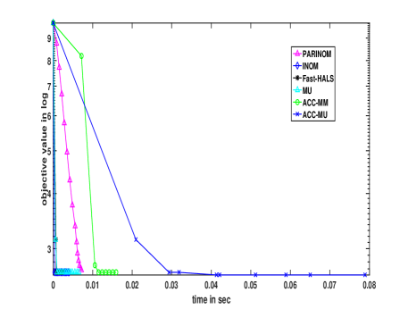
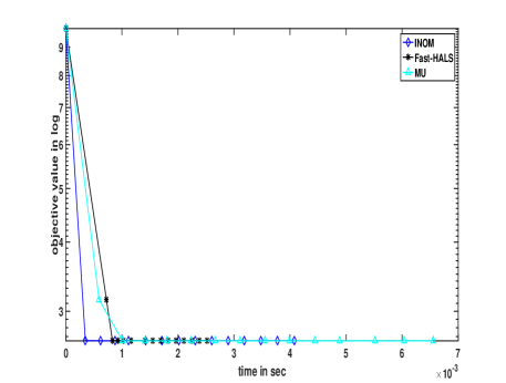
1. In the first simulation, we fix n=100𝑛100n=100, m=200𝑚200m=200 and r=1𝑟1r=1 and compare the convergence rate and per iteration cost of the proposed algorithms vs Fast-HALS, MU and Accelerated MU. The elements of 𝐕𝐕{\mathbf{V}} matrix was randomly generated from a uniform distribution from [100,200]100200[100,200]. Initial values of 𝐖𝐖{\mathbf{W}} and 𝐇𝐇{\mathbf{H}} was also randomly generated from a uniform distribution from [0,1]01[0,1]. The columns of 𝐕𝐕{\mathbf{V}} and 𝐖𝐖{\mathbf{W}} were normalized. The initial objective value fNMF(𝐖0,𝐇0)subscript𝑓NMFsuperscript𝐖0superscript𝐇0f_{{}_{\textrm{NMF}}}({\mathbf{W}}^{0},{\mathbf{H}}^{0}) for all the algorithms were kept same. Fig. 3 (a) shows the run time vs the objective value in log scale of all the algorithms. Fig. 3 (b) compares the run time vs the objective value in log scale of MU, Fast-HALS and INOM.
Refer to caption
(a) Objective value vs run time of the proposed and existing algorithms- Fast-HALS, MU and Accelerated MU
Refer to caption
(b) Objective value vs run time of MU,
Fast-HALS and INOM
Figure 3: Comparison of run time and convergence of proposed algorithm with existing algorithms when n=100𝑛100n=100, m=200𝑚200m=200 and r=1𝑟1r=1.

From Fig. 3(a), it can be seen that the proposed algorithms are monotonic in nature. Accelerated PARINOM has faster convergence when compared to PARINOM algorithm. However, due to the additional steps involved in accelerated PARINOM, the per iteration cost is more in Accelerated PARINOM when compared to PARINOM. From Fig. 3 (b), it can be seen that INOM algorithm takes lesser time to converge when compared to the rest of the algorithms.

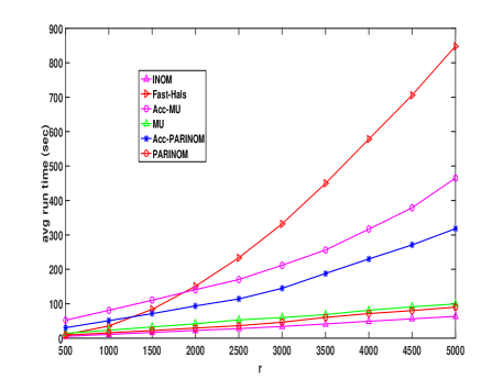
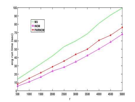
2.a. In this simulation, we compare the proposed algorithms with Fast-HALS, MU and accelerated MU for a dense matrix 𝐕𝐕{\mathbf{V}} with m=50000𝑚50000m=50000 and n=10000𝑛10000n=10000. Dense matrix factorization has application in image processing and in video analysis. The elements of 𝐕𝐕{\mathbf{V}} matrix was randomly generated from a uniform distribution from [100, 200]. Initial values of 𝐖𝐖{\mathbf{W}} and 𝐇𝐇{\mathbf{H}} was randomly generated from a uniform distribution from [0, 1]. The comparison is done based on how quickly the algorithms reduce the initial objective value fNMF(𝐖0,𝐇0)subscript𝑓NMFsuperscript𝐖0superscript𝐇0f_{{}_{\textrm{NMF}}}({\mathbf{W}}^{0},{\mathbf{H}}^{0}) to about 70%percent7070\% of the initial objective value fNMF(𝐖0,𝐇0)subscript𝑓NMFsuperscript𝐖0superscript𝐇0f_{{}_{\textrm{NMF}}}({\mathbf{W}}^{0},{\mathbf{H}}^{0}) for different values of r𝑟r- which was varied from 500500500 to 500050005000 in steps of 500500500. The columns of 𝐕𝐕{\mathbf{V}} and 𝐖𝐖{\mathbf{W}} were normalized. The initial objective value for all the algorithms were kept same. The run time was averaged over 505050 trials. Fig. 4 (a) compares the proposed algorithms with Fast-HALS, MU and accelerated MU algorithm for m=50000𝑚50000m=50000 and n=10000𝑛10000n=10000.

Refer to caption
(a) Comparison of run time of proposed algorithms with Fast-Hals, MU and Acc-MU.
Refer to caption
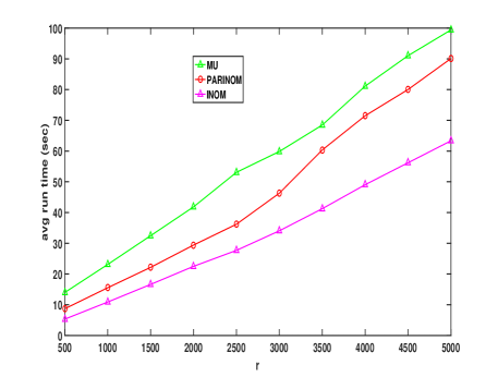
(b) Comparison of run time of MU, INOM and PARINOM
Figure 4: Comparison of proposed algorithm with existing algorithms by varying r𝑟r, m=50000𝑚50000m=50000 and n=10000𝑛10000n=10000 and when 𝐕𝐕{\mathbf{V}} is a dense matrix.

From Fig. 4 (a), it can be seen that as the size of r𝑟r increases, Fast-HALS takes the most time to reduce the initial objective value fNMF(𝐖0,𝐇0)subscript𝑓NMFsuperscript𝐖0superscript𝐇0f_{{}_{\textrm{NMF}}}({\mathbf{W}}^{0},{\mathbf{H}}^{0}) to about 70%percent7070\% of the initial objective value fNMF(𝐖0,𝐇0)subscript𝑓NMFsuperscript𝐖0superscript𝐇0f_{{}_{\textrm{NMF}}}({\mathbf{W}}^{0},{\mathbf{H}}^{0}). Fig.4 (b) compares MU, INOM and PARINOM. From this figure, it can be seen that INOM takes the least time.

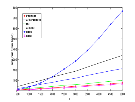
2.b. We repeat the above simulation for a sparse matrix 𝐕𝐕{\mathbf{V}}. Sparse matrix factorization has application in text mining. The elements of a 70%percent7070\% sparse matrix was randomly generated from a normal distribution with negative elements pushed to zero. Fig.5 (a) compares the proposed algorithms with Fast-Hals, MU and accelerated MU algorithm for m=50000𝑚50000m=50000 and n=10000𝑛10000n=10000 when the matrix 𝐕𝐕{\mathbf{V}} is 70%percent7070\% sparse.

Refer to caption
(a) Comparison of run time of proposed algorithms with Fast-Hals, MU and Acc-MU.
Refer to caption
(b) Comparison of run time of MU, INOM and PARINOM
Figure 5: Comparison of proposed algorithm with existing algorithms by varying r𝑟r, m=50000𝑚50000m=50000 and n=10000𝑛10000n=10000 and when 𝐕𝐕{\mathbf{V}} is a 70%percent7070\% sparse matrix

From Fig.5 (a), it can be seen that INOM and PARINOM takes the least time when compared to the state-of-the art algorithms. Also, as the size of r𝑟r increases, Fast-HALS takes the most time to reduce the initial objective value fNMF(𝐖0,𝐇0)subscript𝑓NMFsuperscript𝐖0superscript𝐇0f_{{}_{\textrm{NMF}}}({\mathbf{W}}^{0},{\mathbf{H}}^{0}) to 70%percent7070\% of the initial objective value fNMF(𝐖0,𝐇0)subscript𝑓NMFsuperscript𝐖0superscript𝐇0f_{{}_{\textrm{NMF}}}({\mathbf{W}}^{0},{\mathbf{H}}^{0}). Fig.5 (b) shows only the performance of INOM, PARINOM and MU for better readability.

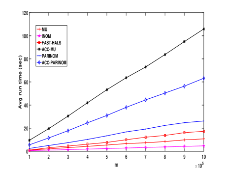
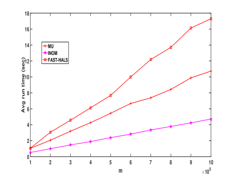
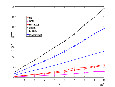
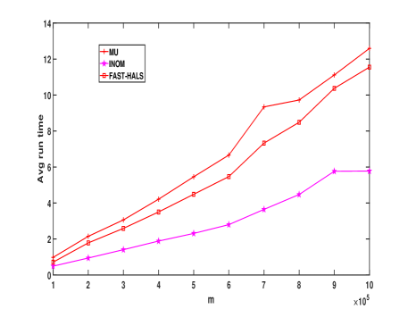
3.a. In this simulation, we vary the size of 𝐕𝐕{\mathbf{V}} and compare the performance of the algorithm. The comparison is done based on how quickly the algorithms reduce the initial objective value fNMF(𝐖0,𝐇0)subscript𝑓NMFsuperscript𝐖0superscript𝐇0f_{{}_{\textrm{NMF}}}({\mathbf{W}}^{0},{\mathbf{H}}^{0}) to about 70%percent7070\% of the initial objective value fNMF(𝐖0,𝐇0)subscript𝑓NMFsuperscript𝐖0superscript𝐇0f_{{}_{\textrm{NMF}}}({\mathbf{W}}^{0},{\mathbf{H}}^{0}). m𝑚m was varied from 100000100000100000 to 100000010000001000000 in steps of 100000100000100000 and n𝑛n and r𝑟r were equal to 100010001000 and 100100100, respectively. The elements of 𝐕𝐕{\mathbf{V}} matrix was randomly generated from a uniform distribution from [100, 200]. Initial values of 𝐖𝐖{\mathbf{W}} and 𝐇𝐇{\mathbf{H}} was randomly generated from a uniform distribution from [0, 1]. The columns of 𝐕𝐕{\mathbf{V}} and 𝐖𝐖{\mathbf{W}} were normalized. The initial objective value for all the algorithms were kept same. The run time was averaged over 505050 trials. Fig. 6 (a) compares the proposed algorithms with Fast-Hals, MU and accelerated MU algorithm for r=100𝑟100r=100 and n=1000𝑛1000n=1000. Fig. 6 (b) compares the performance of INOM, MU and Fast-Hals.
Refer to caption
(a) Comparison of run time of proposed algorithms with Fast-Hals, MU and Acc-MU.
Refer to caption
(b) Comparison of run time of MU, INOM and Fast-Hals
Figure 6: Comparison of proposed algorithm with existing algorithms for varying r𝑟r, m=50000𝑚50000m=50000 and n=10000𝑛10000n=10000 when 𝐕𝐕{\mathbf{V}} is dense matrix.

From Fig.6 (b), it can be seen that INOM takes the least time when compared to the state-of-the art algorithms.

3.b. The above simulation is repeated for a sparse matrix 𝐕𝐕{\mathbf{V}}. The elements of a 70%percent7070\% sparse matrix was randomly generated from a normal distribution with negative elements pushed to zero. Fig.7 (a) compares the proposed algorithms with Fast-Hals, MU and accelerated MU algorithm for r=100𝑟100r=100 and n=1000𝑛1000n=1000. Fig.7 (b) compares the performance of INOM, MU and Fast-Hals. From Fig.7 (b), it can be seen that INOM performs better than MU and Fast-Hals.
Refer to caption
(a) Comparison of run time of proposed algorithms with Fast-Hals, MU and Acc-MU.
Refer to caption
(b) Comparison of run time of MU, INOM and Fast-Hals
Figure 7: Comparison of proposed algorithm with existing algorithms for varying r𝑟r, m=50000𝑚50000m=50000 and n=10000𝑛10000n=10000 when 𝐕𝐕{\mathbf{V}} is 70%percent7070\% sparse matrix.

4. In this simulation, an application of Nonnegative Matrix Factorization on Blind Source Separation(BSS) is shown. In BSS, source signals have to be separated from a set of mixed signals without knowing the mixing process. It is commonly used in audio signal processing, image processing, biomedical signal processing and in digital communications. In the latter case, the 𝐖𝐖{\mathbf{W}} matrix can be thought as the channel response and each row of 𝐇𝐇{\mathbf{H}} consists of the source signal send by the transmitter array. The receiver sensor array then receives a linear mixture of the source signal. The task of BSS is to reconstruct the source signal from the received signal.

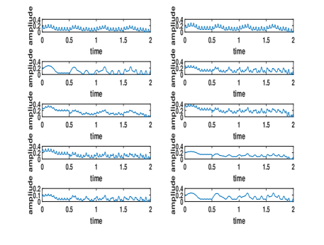
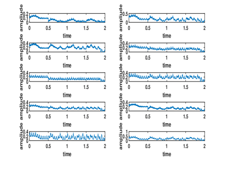
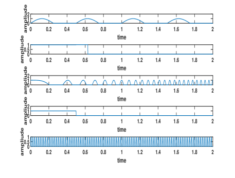
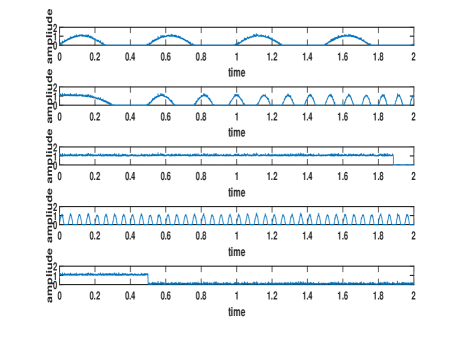
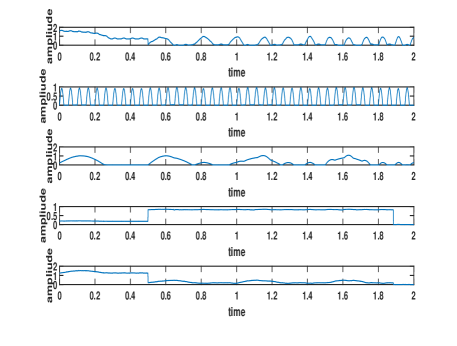
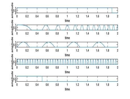
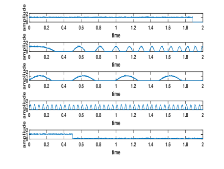
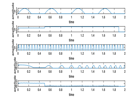
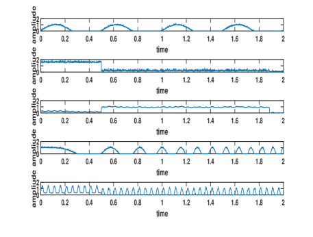
Five source signals for 101010 seconds were simulated-a square wave, a rectangular wave, two sine waves of frequency 222 Hz and 202020 Hz and a chirp signal which begins with 00 Hz at t = 00 sec and cross 303030 Hz after t=5𝑡5t=5 sec. The negative values of the source signals were made zero. 𝐖𝐖{\mathbf{W}} matrix of size 200200200 ×\times 555 was randomly generated. To evaluate the proposed algorithm in presence of noise, random noise with variance 0.010.010.01 was added to the five source signals. Source signals and some of the observed signals are shown in Fig. 8 and Fig. 9 respectively.
Refer to caption
(a)
Refer to caption
(b)
Figure 8: (a) Source signal without noise (b) Noisy source signal with variance = 0.10.10.1
Refer to caption
(a)
Refer to caption
(b)
Figure 9: (a) Observed signal when source signal has no noise. (b) Observed signal when source signal has noise variance = 0.10.10.1

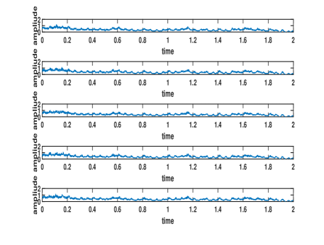
𝐖𝐖{\mathbf{W}} and 𝐇𝐇{\mathbf{H}} were initialized randomly from Uniform distribution from [100, 500] and [200, 400], respectively. The algorithms were made to run till 1000 iterations or unless the relative change in cost function was 108superscript10810^{-8}. Figure. 10 and 11 shows the reconstructed signal by INOM and Fast-Hals, respectively. MU algorithm was not able to reconstruct the signal in the presence of noise and the same is shown in Fig. 12.
Refer to caption
(a)
Refer to caption
(b)
Figure 10: Reconstructed signal by INOM (a) without noise. (b) with noise variance = 0.10.10.1
Refer to caption
(a)
Refer to caption
(b)
Figure 11: Reconstructed signal by Fast-Hals (a) without noise (b) with noise variance = 0.10.10.1
Refer to caption
(a)
Refer to caption
(b)
Figure 12: Reconstructed signal by MU (a) without noise (b) with noise variance = 0.10.10.1

V Possible Extension and Conclusion

In this paper, we proposed two different MM based algorithms - INOM and PARINOM to solve the NMF problem. INOM sequentially updates the 𝐖𝐖{\mathbf{W}} and 𝐇𝐇{\mathbf{H}} matrices, while PARINOM parallely updates them. The update equations of 𝐖𝐖{\mathbf{W}} and 𝐇𝐇{\mathbf{H}} matrices in case of INOM resembles the update equation of Gradient Descent algorithms with adaptive step sizes. We also prove that the proposed algorithms are monotonic and converge to the stationary point of the NMF problem. Various computer simulations were performed to compare the proposed algorithms with the existing algorithms. It was found that INOM performed better than existing algorithms.

The effect of parallel update will be predominantly visible when one has to decompose a multidimensional array into matrices of varied dimensions. This problem is called NonNegative Tensor Factorization (NTF) [40], [41], [42], [43]. A brief overview of NTF is given below.

Suppose, a tensor X of order N m1×m2mNsuperscriptsubscript𝑚1subscript𝑚2subscript𝑚𝑁\mathbb{R}^{{m_{1}\times{m_{2}}}\cdots{m_{N}}} is given. This can be represented as sum of rank one tensors i.e.

𝐗=k=1K𝐚𝐤(1)𝐚𝐤(2)𝐚𝐤(N)𝐗superscriptsubscript𝑘1𝐾tensor-productsuperscriptsubscript𝐚𝐤1superscriptsubscript𝐚𝐤2superscriptsubscript𝐚𝐤𝑁missing-subexpression\begin{array}[]{ll}\mathbf{X}=\displaystyle\sum_{k=1}^{K}{\mathbf{a_{k}}}^{(1)}\otimes{\mathbf{a_{k}}}^{(2)}\cdots{\mathbf{a_{k}}^{(N)}}\end{array} (45)

where 𝐚𝐤(1)superscriptsubscript𝐚𝐤1{\mathbf{a_{k}}}^{(1)} belongs to m1superscriptsubscript𝑚1\mathbb{R}^{m_{1}}, 𝐚(𝐤)(2)superscriptsubscript𝐚𝐤2{\mathbf{a_{(k)}}}^{(2)} belongs to m2superscriptsubscript𝑚2\mathbb{R}^{m_{2}} and so on. K is rank of the tensor and tensor-product\otimes represents outer product. This can be written in a compact form as:

𝐗=[𝐀(1),𝐀(2)𝐀(N)]𝐗superscript𝐀1superscript𝐀2superscript𝐀𝑁missing-subexpression\begin{array}[]{ll}\mathbf{X}=[\mathbf{A}^{(1)},\mathbf{A}^{(2)}\cdots\mathbf{A}^{(N)}]\end{array} (46)

where 𝐀(1)=[𝐚𝟏(1),𝐚𝟐(1),,𝐚𝐊(1)]superscript𝐀1superscriptsubscript𝐚11superscriptsubscript𝐚21superscriptsubscript𝐚𝐊1{\mathbf{A}}^{(1)}=[{\mathbf{a_{1}}}^{(1)},{\mathbf{a_{2}}}^{(1)},\cdots,{\mathbf{a_{K}}}^{(1)}] is of size m1×Ksubscript𝑚1𝐾m_{1}\times K. Similarly, 𝐀(2)=[𝐚𝟏(2),𝐚𝟐(2),,𝐚𝐊(2)]superscript𝐀2superscriptsubscript𝐚12superscriptsubscript𝐚22superscriptsubscript𝐚𝐊2{\mathbf{A}}^{(2)}=[{\mathbf{a_{1}}}^{(2)},{\mathbf{a_{2}}}^{(2)},\cdots,{\mathbf{a_{K}}}^{(2)}] and is of size m2×Ksubscript𝑚2𝐾m_{2}\times K. [𝐀(1),𝐀(2)𝐀(N)]superscript𝐀1superscript𝐀2superscript𝐀𝑁[\mathbf{A}^{(1)},\mathbf{A}^{(2)}\cdots\mathbf{A}^{(N)}] represents k=1K𝐚𝐤(1)𝐚𝐤(2)𝐚𝐤(N)superscriptsubscript𝑘1𝐾tensor-productsuperscriptsubscript𝐚𝐤1superscriptsubscript𝐚𝐤2superscriptsubscript𝐚𝐤𝑁\sum_{k=1}^{K}{\mathbf{a_{k}}}^{(1)}\otimes{\mathbf{a_{k}}}^{(2)}\cdots{\mathbf{a_{k}}^{(N)}}. Hence, the NTF problem can be formulated as:

NTF:minimize𝐀(1),𝐀(2)𝐀(N)0(𝐗[𝐀(1),𝐀(2)𝐀(N)]F2)NTF:superscript𝐀1superscript𝐀2superscript𝐀𝑁0minimizesuperscriptsubscriptnorm𝐗superscript𝐀1superscript𝐀2superscript𝐀NF2missing-subexpression\begin{array}[]{ll}\textrm{NTF:}\quad\underset{\mathbf{A}^{(1)},\mathbf{A}^{(2)}\cdots\mathbf{A}^{(N)}\geq 0}{\rm minimize}\>\left(\|\mathbf{X}-[\mathbf{A}^{(1)},\mathbf{A}^{(2)}\cdots\mathbf{A}^{(N)}]\|_{F}^{2}\right)\end{array} (47)

When compared to parallel update of matrices, alternating minimization will definitely take significantly more time to solve the problem. Since NTF is a generalization of NMF, the proposed algorithms can also be applied to solve NTF and the parallel update algorithm - PARINOM would be more handy for NTF.

References

  • [1] S. Kaski and J. Peltonen, “Dimensionality reduction for data visualization [applications corner],” IEEE Signal Processing Magazine, vol. 28, no. 2, pp. 100–104, 2011.
  • [2] G. Strang, Linear Algebra and Its Applications.   Thomson, Brooks/Cole, 2006.
  • [3] B. Moore, “Principal component analysis in linear systems: Controllability, observability, and model reduction,” IEEE Transactions on Automatic Control, vol. 26, no. 1, pp. 17–32, 1981.
  • [4] B. Thompson, “Factor analysis,” The Blackwell Encyclopedia of Sociology, 2007.
  • [5] P. Smaragdis and J. C. Brown, “Non-negative matrix factorization for polyphonic music transcription,” vol. 3, no. 3, pp. 177–180, 2003.
  • [6] V. P. Pauca, F. Shahnaz, M. W. Berry, and R. J. Plemmons, “Text mining using non-negative matrix factorizations,” pp. 452–456, 2004.
  • [7] J. Zhang, L. Wei, Q. Miao, and Y. Wang, “Image fusion based on nonnegative matrix factorization,” vol. 2, pp. 973–976, 2004.
  • [8] P. Fernsel and P. Maass, “A survey on surrogate approaches to non-negative matrix factorization,” arXiv preprint arXiv:1808.01975, 2018.
  • [9] D. Donoho and V. Stodden, “When does non-negative matrix factorization give a correct decomposition into parts?” pp. 1141–1148, 2004.
  • [10] S. Essid, “A single-class SVM based algorithm for computing an identifiable NMF,” pp. 2053–2056, 2012.
  • [11] J. Kim, Y. He, and H. Park, “Algorithms for nonnegative matrix and tensor factorizations: A unified view based on block coordinate descent framework,” Journal of Global Optimization, vol. 58, no. 2, pp. 285–319, 2014.
  • [12] Y. Xu and W. Yin, “A globally convergent algorithm for nonconvex optimization based on block coordinate update,” Journal of Scientific Computing, vol. 72, no. 2, pp. 700–734, 2017.
  • [13] S. Bonettini, “Inexact block coordinate descent methods with application to non-negative matrix factorization,” IMA Journal of Numerical Analysis, vol. 31, no. 4, pp. 1431–1452, 2011.
  • [14] D. D. Lee and H. S. Seung, “Algorithms for non-negative matrix factorization,” in Advances in neural information processing systems, 2001, pp. 556–562.
  • [15] E. F. Gonzalez and Y. Zhang, “Accelerating the Lee-Seung algorithm for nonnegative matrix factorization,” Tech. Rep., 2005.
  • [16] C.-J. Lin, “Projected gradient methods for nonnegative matrix factorization,” Neural computation, vol. 19, no. 10, pp. 2756–2779, 2007.
  • [17] N.-D. Ho, P. Van Dooren, and V. D. Blondel, “Descent methods for nonnegative matrix factorization,” pp. 251–293, 2011.
  • [18] T. D. Hien, D. Van Tuan, and P. Van At, “Additive update algorithm for nonnegative matrix factorization,” arXiv preprint arXiv:1209.5647, 2012.
  • [19] A. Cichocki, R. Zdunek, and S.-i. Amari, “Nonnegative matrix and tensor factorization [lecture notes],” IEEE Signal Processing Magazine, vol. 25, no. 1, pp. 142–145, 2008.
  • [20] H. Kim and H. Park, “Nonnegative matrix factorization based on alternating nonnegativity constrained least squares and active set method,” SIAM journal on matrix analysis and applications, vol. 30, no. 2, pp. 713–730, 2008.
  • [21] J. Kim and H. Park, “Toward faster nonnegative matrix factorization: A new algorithm and comparisons,” pp. 353–362, 2008.
  • [22] M. H. Van Benthem and M. R. Keenan, “Fast algorithm for the solution of large-scale non-negativity-constrained least squares problems,” Journal of Chemometrics: A Journal of the Chemometrics Society, vol. 18, no. 10, pp. 441–450, 2004.
  • [23] N. Gillis et al., “Nonnegative matrix factorization: Complexity, algorithms and applications,” Unpublished doctoral dissertation, Université catholique de Louvain. Louvain-La-Neuve: CORE, 2011.
  • [24] A. Cichocki, R. Zdunek, and S.-i. Amari, “Hierarchical als algorithms for nonnegative matrix and 3d tensor factorization,” International Conference on Independent Component Analysis and Signal Separation, pp. 169–176, 2007.
  • [25] A. Cichocki and A.-H. Phan, “Fast local algorithms for large scale nonnegative matrix and tensor factorizations,” IEICE transactions on Fundamentals of Electronics, Communications and Computer sciences, vol. 92, no. 3, pp. 708–721, 2009.
  • [26] D. Hajinezhad, T.-H. Chang, X. Wang, Q. Shi, and M. Hong, “Nonnegative matrix factorization using ADMM: Algorithm and convergence analysis,” pp. 4742–4746, 2016.
  • [27] S. Boyd, N. Parikh, E. Chu, B. Peleato, J. Eckstein et al., “Distributed optimization and statistical learning via the alternating direction method of multipliers,” Foundations and Trends in Machine learning, vol. 3, no. 1, pp. 1–122, 2011.
  • [28] A. Vandaele, N. Gillis, F. Glineur, and D. Tuyttens, “Heuristics for exact nonnegative matrix factorization,” Journal of Global Optimization, vol. 65, no. 2, pp. 369–400, 2016.
  • [29] Y. Sun, P. Babu, and D. P. Palomar, “Majorization-minimization algorithms in signal processing, communications, and machine learning,” IEEE Transactions on Signal Processing, vol. 65, no. 3, pp. 794–816, 2017.
  • [30] D. R. Hunter and K. Lange, “A tutorial on MM algorithms,” The American Statistician, vol. 58, no. 1, pp. 30–37, 2004.
  • [31] D. Böhning and B. G. Lindsay, “Monotonicity of quadratic-approximation algorithms,” Annals of the Institute of Statistical Mathematics, vol. 40, no. 4, pp. 641–663, 1988.
  • [32] S. U. Pillai, T. Suel, and S. Cha, “The Perron-Frobenius theorem: some of its applications,” IEEE Signal Processing Magazine, vol. 22, no. 2, pp. 62–75, 2005.
  • [33] S. Gaubert and J. Gunawardena, “The Perron-Frobenius theorem for homogeneous, monotone functions,” Transactions of the American Mathematical Society, vol. 356, no. 12, pp. 4931–4950, 2004.
  • [34] W. Sun and Y.-X. Yuan, Optimization theory and methods: nonlinear programming.   Springer Science & Business Media, 2006, vol. 1.
  • [35] C. D. Maranas and C. A. Floudas, “Global optimization in generalized geometric programming,” Computers & Chemical Engineering, vol. 21, no. 4, pp. 351–369, 1997.
  • [36] K. Lange and H. Zhou, “MM algorithms for geometric and signomial programming,” Mathematical programming, vol. 143, no. 1-2, pp. 339–356, 2014.
  • [37] S. Boyd and L. Vandenberghe, Convex optimization.   Cambridge university press, 2004.
  • [38] M. Razaviyayn, M. Hong, and Z.-Q. Luo, “A unified convergence analysis of block successive minimization methods for nonsmooth optimization,” SIAM Journal on Optimization, vol. 23, no. 2, pp. 1126–1153, 2013.
  • [39] R. Varadhan and C. Roland, “Simple and globally convergent methods for accelerating the convergence of any EM algorithm,” Scandinavian Journal of Statistics, vol. 35, no. 2, pp. 335–353, 2008.
  • [40] Y. Qian, F. Xiong, S. Zeng, J. Zhou, and Y. Y. Tang, “Matrix-vector nonnegative tensor factorization for blind unmixing of hyperspectral imagery,” IEEE Transactions on Geoscience and Remote Sensing, vol. 55, no. 3, pp. 1776–1792, 2017.
  • [41] N. B. Erichson, A. Mendible, S. Wihlborn, and J. N. Kutz, “Randomized nonnegative matrix factorization,” Pattern Recognition Letters, vol. 104, pp. 1–7, 2018.
  • [42] A. Sapienza, A. Bessi, and E. Ferrara, “Non-negative tensor factorization for human behavioral pattern mining in online games,” Information, vol. 9, no. 3, p. 66, 2018.
  • [43] N. D. Sidiropoulos, L. De Lathauwer, X. Fu, K. Huang, E. E. Papalexakis, and C. Faloutsos, “Tensor decomposition for signal processing and machine learning,” IEEE Transactions on Signal Processing, vol. 65, no. 13, pp. 3551–3582, 2017.