Supritam Bhattacharjeesupritamb@iisc.ac.in1
\addauthorDevraj Mandaldevrajm@iisc.ac.in1
\addauthorSoma Biswassomabiswas@iisc.ac.in1
\addinstitution
Department of Electrical Engineering
Indian Institute of Science
Bangalore, India-560012.
Multi-class Novelty Detection Using Mix-up Technique
Multi-class Novelty Detection Using Mix-up Technique
Abstract
Multi-class novelty detection is increasingly becoming an important area of research due to the continuous increase in the number of object categories. It tries to answer the pertinent question: given a test sample, should we even try to classify it? We propose a novel solution using the concept of mixup technique for novelty detection, termed as Segregation Network. During training, a pair of examples are selected from the training data and an interpolated data point using their convex combination is constructed. We develop a suitable loss function to train our model to predict its constituent classes. During testing, each input query is combined with the known class prototypes to generate mixed samples which are then passed through the trained network. Our model which is trained to reveal the constituent classes can then be used to determine whether the sample is novel or not. The intuition is that if a query comes from a known class and is mixed with the set of known class prototypes, then the prediction of the trained model for the correct class should be high. In contrast, for a query from a novel class, the predictions for all the known classes should be low. The proposed model is trained using only the available known class data and does not need access to any auxiliary dataset or attributes. Extensive experiments on two benchmark datasets, namely Caltech 256 and Stanford Dogs and comparisons with the state-of-the-art algorithms justifies the usefulness of our approach.
1 Introduction
Deep learning approaches have achieved impressive performance for object recognition and classification task [Krizhevsky et al.(2012)Krizhevsky, Sutskever, and Hinton] [Simonyan and Zisserman(2014)] by using large networks trained with millions of data examples. However, these networks usually work under a closed set assumption, and thus tries to classify each query sample, even if it does not belong to one of the training classes. For example, a neural network classifier trained to classify fruits, might classify an input from a completely different category, say “bird” into one of the fruit classes with high confidence, which is unlikely to happen if a human does the same task. To make the systems more intelligent and better suited to real-world applications [Pimentel et al.(2014)Pimentel, Clifton, Clifton, and Tarassenko] [Markou and Singh(2003)], they should be able to understand whether the input belongs to one of the trained classes before trying to classify it.
This problem is addressed in recent literature as out-of-distribution detection [DeVries and Taylor(2018)], anomaly detection [Zong et al.(2018)Zong, Song, Min, Cheng, Lumezanu, Cho, and Chen], novelty detection [Mohammadi-Ghazi et al.(2018)Mohammadi-Ghazi, Marzouk, and Büyüköztürk] [Abati et al.(2019)Abati, Porrello, Calderara, and Cucchiara] and one-class classification [Perera et al.(2019)Perera, Nallapati, and Xiang] [Sadooghi and Khadem(2018)], each having subtle differences between them. One class classification rejects all the classes as outliers except the concerned class. In out-of-distribution paradigm, the algorithm determines whether samples are coming from other data-sets or distribution. Such algorithms often require the availability or prior knowledge about the out-of-distribution data for its proper functioning.
In this work, we address the multi-class novelty detection task [Perera and Patel(2019)], where given a query, the goal is to understand whether it belongs to one of the training classes. This is very challenging, since the novel data can come from the same data distribution as that of the training data. Here, we propose a novel framework, termed Segregation Network, which utilizes the mixup technique [Tokozume et al.(2018)Tokozume, Ushiku, and Harada] for this task. The network takes as input a pair of data points, and a third interpolated data point which is generated by mixing them together using a variable ratio. The goal is to determine the constituent classes and the respective proportions by which the two inputs have been mixed to generate the interpolated data point. To this end, we design a novel loss function called Constituency loss for our objective. Once the network is trained, given an unknown query, we mix it with the known class prototypes in a predefined proportion and pass it through the network. Based on the network output, we infer whether the query belongs to the known set of classes or a novel class unknown to the system. The main contributions of our work are as follows:
-
•
We propose a novelty detection framework, termed as Segregation Network, which uses the mixup technique, to detect whether the test query belongs to one of the known classes or to a novel class.
-
•
We design a novel loss function called Constituency loss to train the proposed Segregation Network.
-
•
The proposed network can be trained only using the available training data and does not require access to any auxiliary or out-of-distribution dataset as in done in similar methods like [Perera and Patel(2019)]. This is advantageous as the collection of auxiliary data is often difficult, expensive and might be data dependent with respect to the known class set.
-
•
During testing, the proposed network compares the unknown query with the set of known class prototypes. We also develop an efficient version of our algorithm, without any significant drop in performance, which utilizes the softmax confidence outputs of the pre-trained network.
-
•
We perform experiments on two standard benchmark datasets for novelty detection and the results obtained compare favorably with the state-of-the-art method which leverages auxiliary training data.
2 Related Work
The foundation of this work is based on two threads of machine learning research, namely novelty detection algorithm and mix-up based learning techniques.
Novelty Detection: This problem is an active area of research for detecting outliers in data.
There have been both statistical [Stevens(1984)] [Yamanishi et al.(2004)Yamanishi, Takeuchi, Williams, and
Milne] [Kim and Scott(2012)] [Eskin(2000)], distance based [Knorr et al.(2000)Knorr, Ng, and Tucakov] [Hautamaki et al.(2004)Hautamaki, Karkkainen, and
Franti] [Eskin et al.(2002)Eskin, Arnold, Prerau, Portnoy, and
Stolfo] and deep learning based approaches [Pidhorskyi et al.(2018)Pidhorskyi, Almohsen, and
Doretto] [Akcay et al.(2018)Akcay, Atapour-Abarghouei, and
Breckon] [Lee et al.(2018)Lee, Lee, Min, Zhang, Shin, and
Lee].
Statistical methods generally focus on trying to fit the distribution of the known data using probability models [Clifton et al.(2011)Clifton, Hugueny, and
Tarassenko].
Distance based algorithms generally use some transform and then identify novel classes by thresholding the distance with known examples.
The assumption is that the known class examples will be much closer to the known class representatives, than the unknown ones, in the transformed space.
A relatively recent work in this direction is Kernel-Null Foley-Sammon Transform (KNFST) [Bodesheim et al.(2013)Bodesheim, Freytag, Rodner, Kemmler, and
Denzler] for multi-class novelty detection.
Here the same class points are projected into a single point in the null space, and during testing, the distance with respect to the class representative is thresholded to get a novelty score.
This algorithm was improved to handle incremental incoming classes and subsequently update its novelty detector in [Liu et al.(2017)Liu, Lian, Wang, and Xiao].
Deep learning based approaches such as Open-max [Bendale and Boult(2016)] tries to fit a Weibull-distribution to determine the novelty. The generative version of this approach was proposed in [Ge et al.(2017)Ge, Demyanov, Chen, and Garnavi], where unknown samples were generated.
Several one-class deep learning based novelty detection has been proposed in recent literature [Sabokrou et al.(2018)Sabokrou, Khalooei, Fathy, and
Adeli] [Perera et al.(2019)Perera, Nallapati, and Xiang] [Sadooghi and Khadem(2018)].
The work in [Perera and Patel(2019)] designs a novel training paradigm where a reference set is used to learn a set of negative filters that will not be activated for the known category data. To this end they design a novel loss function called membership loss.
Masana et al. [Masana et al.(2018)Masana, Ruiz, Serrat, van de Weijer, and
Lopez] propose a method to improve the feature space by forming discriminative features with contrastive loss for this task.
Out-of-Distribution detection algorithms [DeVries and Taylor(2018)] [Liang et al.(2017)Liang, Li, and Srikant] [Vyas et al.(2018)Vyas, Jammalamadaka, Zhu, Das, Kaul, and
Willke] also addresses a similar task, having subtle difference with the problem addressed in this work.
These approaches assume that the novel or out of distribution data is strictly outside the data manifold on which the base network is trained.
Thus, novelty detection is in general more challenging than out of distribution detection [Perera and Patel(2019)].
Mixing: Learning algorithms involving interpolation or mix-up between classes has been recently introduced in the community.
In one of the early works, Bengio et al. [Bengio et al.(2013)Bengio, Mesnil, Dauphin, and
Rifai] employed mixing technique to better understand the underlying factor of disentanglement in data.
Recently, [Tokozume et al.(2018)Tokozume, Ushiku, and
Harada] proposed to improve the classification task by interpolating between classes. In [Tokozume et al.(2017)Tokozume, Ushiku, and
Harada], sound recognition is done by feeding data between class (or mixed up) samples to improve the performance.
Another work along similar lines is proposed in [Zhang et al.(2018)Zhang, Cisse, Dauphin, and
Lopez-Paz].
While the mentioned works interpolate in the input space, [Berthelot et al.(2019)Berthelot, Raffel, Roy, and
Goodfellow] interpolated in the latent space of auto-encoders to generate images with smooth transition from one class to another using adversarial regularizer.
Several other works tries to interpolate or mix data from different class in the the latent space of auto-encoders [Dumoulin et al.(2017)Dumoulin, Belghazi, Poole, Mastropietro, Lamb,
Arjovsky, and Courville] [Mathieu et al.(2016)Mathieu, Zhao, Zhao, Ramesh, Sprechmann, and
LeCun] [Ha and Eck(2018)] [Bowman et al.(2015)Bowman, Vilnis, Vinyals, Dai, Jozefowicz, and
Bengio] [Mescheder et al.(2017)Mescheder, Nowozin, and
Geiger] for different purposes and using various methods.
In contrast, in our work, we interpolate in the feature space to train our model.
3 Motivation
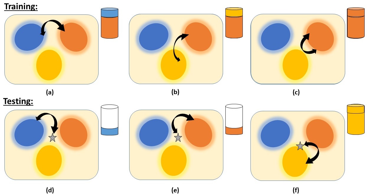
The basic idea behind the development of the algorithm is provided in Figure 1, where we highlight our training (top row) and testing (bottom row) strategies. The different color schemes indicate the different categories of data. The bi-directional arrow indicates that samples from these two categories are being used to generate the interpolated data point. The desired prediction of our trained model is shown in a color-coded bin.
During training, the proposed network aims to segregate the interpolated point with respect to the two inputs. For the example shown in Figure 1(a, b), the interpolated point lies close to the orange class since higher mixing coefficient has been used for that class. So our model should ideally predict the constituent classes (as shown in the color coded bins) with higher weightage to the orange class. In Figure 1(c), the interpolated point should be predicted to belong to only the orange class, as two samples from the orange class have been used to generate the interpolated point.
During testing (as shown in bottom row), we generate the interpolated point using the query (denoted as gray star) and the class prototypes of the known classes, and try to predict the constituent classes with respect to the two input points. We give a larger weightage to the query while generating the interpolated point. In Figure 1(d,e), since the query does not belong to any of the known class set, the prediction of the network should consist of only the known class mixing coefficient (shown in the color bins). In case the query comes from the known set (yellow class in Figure 1(f)), the prediction of our network should ideally reflect that with a high value in the color coded bin. Thus the output of the network can be used to determine whether the input belongs to one of the known classes or to a novel class.

4 Proposed Method
In this section, we describe the network architecture of the proposed Segregation Network, the novel loss function used to train the model and the training and testing protocol.
First, we describe the notations used.
Notations: Let the input data be represented as , being the number of training samples and being its feature dimension.
Let the labels be denoted as , where is the number of training or known classes.
We define the known class set to be , and thus .
In the general scenario, the testing data can come from the seen classes or from unseen/novel classes, for which no information is available to the system.
During testing, given a query, the goal is to determine whether it comes from set or not, i.e. whether it belongs to a seen class or a novel class.
Classifying the known examples into its correct class is not the focus of this work and can be done using the base classifier trained using the training data.
Base Classifier and Features: Given the training data, a base classifier is trained to classify an input query into one of the given classes.
Since the classifier is now required to work in a general setting, the input can potentially come from an unseen class, and thus should not be classified by the classifier into one of the seen classes.
Given an input, the novelty detector is designed to take the output features of the classifier (before they are classified) and decide whether the input belongs to one of the seen classes or to a novel class.
If it belongs to a seen class, it can be send back to the classifier for classification.
The proposed novelty detection framework is general and can work with any classifier model.
In this work, we use pre-trained Alexnet [Krizhevsky et al.(2012)Krizhevsky, Sutskever, and Hinton] and VGG16 [Simonyan and Zisserman(2014)] architecture as the base classifier.
These networks are fine-tuned on the respective known class datasets and the extracted features are normalized and given as input to our network.
Now, we describe the details of the Segregation Network.
4.1 Segregation Network
The proposed network consists of three fully connected (fc) layers with ReLU activations and dropout between each layer except the final fc layer. The final layer is of dimension (number of seen classes). Sigmoid is used as the final layer activation function as the output of Sigmoid is between which can be interpreted as the proportion of the mixing classes in our case. In our design, the network has a architecture, with the numbers denoting the length of each fc layer. We use the Adam optimizer with a learning rate of 0.001 for training our model. An illustration of the proposed network is shown in Figure 2.
The network takes as input a triplet set of data samples , where , are data from the training set and is the mixture obtained by mixing and in some proportion.
Let us denote the output of the first fc layer, which is shared by all three inputs, as .
Then is concatenated together to form which is then passed forward through the rest of the network.
In our implementation, we have used features from the fine-tuned Alexnet [Krizhevsky et al.(2012)Krizhevsky, Sutskever, and Hinton] or VGG16 [Simonyan and Zisserman(2014)] deep networks, which are of very high dimension.
Thus, the first fc layer serves as a dimensionality reduction layer, the output of which is then concatenated and passed through the rest of the network structure.
The final output of the network after passing through the sigmoid activation function is denoted as .
Training the model :
The network is trained such that given an interpolated input, it will decouple/segregate the input data into its constituents.
This property is exploited in the following way.
Given a pair of feature vectors , we perform convex combination on this pair to produce , where , .
We feed these three feature vectors to our network.
The output of the network is a dimensional vector from the final sigmoid layer .
Since the output is passed through the sigmoid activation function, each element of the -dimensional vector is bounded between .
In addition, each element denotes the proportion by which the mixed sample has been constructed from that training class.
For example, an output of (i.e. there are five known classes) indicates that the mixed sample has been constructed as where and .
Given , the following cases may arise,
-
•
If, and , where , and both , i.e., belongs to the seen classes set, we should get the output of the model such that, and , while for . We consider such a pair to be a non-matched pair as the interpolated point lies somewhere in between the two classes based on the value of .
-
•
If, both , , the network should ideally output and for . This is because a mixed element constructed from two data items of the same class should ideally belong to the same class also. We consider such a pair to be a matched pair.
-
•
During testing in general scenario, we pair the query sample with class prototypes of the known classes, and so a third case may arise if the query belongs to a novel class. Here, since one of the two inputs to the network is seen, only the output node corresponding to that class should be non-zero and equal to the proportion of this class in the generated mixture. We do not explicitly train the network for this scenario, since we do not assume any auxiliary dataset. So, we consider only the first two cases for training.
Note that as the final activation function is the sigmoid layer and not the standard softmax, total sum of may not be equal to . This is important, since if the input belongs to a novel class, the network will only consider the mixing proportion of the known class. So the proportion of unknown class in the mixture will be ignored and thus the sum will not be equal to 1.
Our network needs to be trained in such a way that the value of peaks at the position of the constituent classes and also gives the proper mixing proportions.
Since, we do not have the softmax output, we cannot use cross-entropy loss function to train this model.
In addition, cross-entropy loss function tries to maximize the probability of a sample to belong to a particular class which goes against our desired objective, where a given example can come from outside the known class set.
Hence, we design a novel loss function termed as Constituency loss () to train our model which we describe next.
Constituency loss: This loss ensures that the output of the Segregation Network, , gives positive values for only those classes which has been mixed to create .
Thus, the network is expected to output not only the correct proportion over the mixing class set , but also give zero output over the non-mixing class set .
Based on this requirement, the loss function can be written for the and classes as follows
| (1) |
where, denotes the mixing coefficient vector which has zeros for the non-mixing classes, and values of and in their relevant places for the mixing classes. Let us define and denote the zero element and non-zero element sets. The set denotes the sparse set of output for the non-mixing classes, while the is for the classes used to form . The weight plays a significant role in training the model as shown in the ablation studies. This factor is important since , where denotes the cardinality of a set. Hence during training, we penalize the errors in wrongly predicting the value of much more severely as compared to the incorrect prediction of the zero elements. In our implementation, we found the best value of to be between in all our experiments.
4.2 Testing Scenario
As mentioned earlier, we assume that a base pre-trained classifier has been fine-tuned on the training classes with a softmax output layer. Here, it has been taken as the AlexNet [Krizhevsky et al.(2012)Krizhevsky, Sutskever, and Hinton] or VGG16 [Simonyan and Zisserman(2014)] from where the features are extracted. In the general testing scenario, the test query can come from one of the seen classes or from a novel class. Given a test query, we consider the Top-N classes which get the highest output scores from the classifier, i.e. the possibility of the query belonging to one of these classes is high. The goal of the Segregation Network is to consider each of these top classes, and verify whether the query actually belongs to one of those classes. Taking the top few classes is intuitive since (1) if the query belongs to a seen class, its score is usually high and (2) it reduces the computation required for novelty detection using the proposed Segregation Network. If the query is from a novel class, all retrieved classes are obviously wrong. Here we use training class centers, where , where () as the prototype exemplars. For each query, , a set of interpolated points is generated as , where , which is then is passed through the proposed network. The prediction using all exemplar points can be viewed as a square matrix (shown in Figure 3) whose each row signifies the prediction values when paired with a particular cluster center.
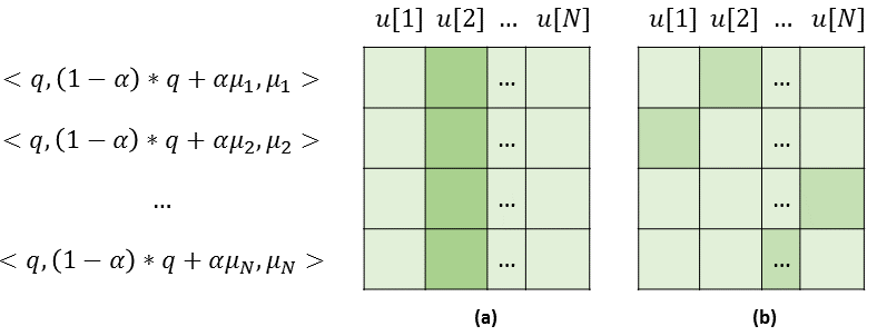
The mixing coefficient for the prototype exemplars are kept low while feeding to our model. In other words the mixing coefficient is kept high for the incoming test data. This is because of the following reasons
-
•
If the query data belongs to one of the known classes, the high value for the query example would produce a high value for the correct known class as shown in Figure 3 (a).
-
•
If the query data belongs to an unknown class, the low value used for the prototype exemplars forces the network output to be low for all the (known) classes (as shown in Figure 3 (b)).
We define the membership score as the average of the maximum score in each row. Membership score can be thought of as the likelihood of belonging to the set of known classes. Thus, for a query coming from the known classes, the membership score should be higher as compared to the membership score of a query coming from the novel class set. As seen in Figure 3(a), the individual maximum values of the prediction matrix per row is higher (marked with a deep green shade) and so the membership score (the average value) is higher. When the query belongs to the novel set, as seen in Figure 3(b), the membership score would come out to be lower.
5 Experiments
In this section, we evaluate our method termed as Mixing Novelty Detector (MND) and compare against several state-of-the-art approaches. We describe in details the datasets considered for our experiments and the testing protocol. This is followed by ablation studies to better understand our proposed method.
5.1 Datasets Used and Testing Protocol
Here, we report results on two benchmark datasets, namely Caltech 256 [Griffin et al.(2007)Griffin, Holub, and Perona] and Stanford Dogs [Khosla et al.(2011)Khosla, Jayadevaprakash, Yao, and Li].
Caltech 256 dataset [Griffin et al.(2007)Griffin, Holub, and Perona]: This dataset is a standard dataset for visual recognition consisting of objects spread over diverse categories. It consists of images with a minimum of to a maximum of image examples per class. As per the protocol in [Perera and Patel(2019)], we took the first classes as known and rest as unknown.
Stanford Dogs dataset [Khosla et al.(2011)Khosla, Jayadevaprakash, Yao, and Li]: This is a fine grained dataset which has been curated from the ImageNet dataset and consists of images of different breeds of dogs of categories.
It consists of total of images.
We consider the first classes, sorted alphabetically as known.
The final testing was performed on the remaining classes, similar to the protocol followed in [Perera and Patel(2019)].
State-of-the-art Approaches in Literature:
We justify the effectiveness of our proposed model for the task of multi-class novelty detection by comparing against the following current state-of-the-art approaches:
(1) Finetune [Simonyan and Zisserman(2014)]: The fine-tuned network output is taken and thresholded to determine whether a query belongs to the known or novel class;
(2) One-class SVM [Schölkopf et al.(2001)Schölkopf, Platt, Shawe-Taylor, Smola,
and Williamson]: All known classes are considered during training the SVM. During testing the maximum SVM score is considered for determining whether a data-point is novel or not.
(3) KNFST [Bodesheim et al.(2013)Bodesheim, Freytag, Rodner, Kemmler, and
Denzler]: The deep features are extracted and normalized and the KNFST algorithm is implemented to project all the training samples into the null space, where all examples from a particular class collapse to a single point. Finally, the distance of a query from the training class in the null space is thresholded to determine whether it is novel or not;
(4) Local KNFST [Bodesheim et al.(2015)Bodesheim, Freytag, Rodner, and
Denzler]: This method is similar to that in [Bodesheim et al.(2013)Bodesheim, Freytag, Rodner, Kemmler, and
Denzler], but focuses only on the training images most similar to the given query for determining its novelty score;
(5) Openmax [Bendale and Boult(2016)]: The feature embedding of the penultimate layer of a trained network is taken and mean activation vectors are determined to fit in the Weibull distribution to finally generate a probability vector of dimension , where is the number of classes.
(6) K-extremes [Schultheiss et al.(2017)Schultheiss, Käding, Freytag, and
Denzler]: VGG16 features are extracted and the top activation index is used to get the extreme value signatures;
(7) Finetune () [Perera and Patel(2019)]: The network is trained on additional classes from a reference dataset which has examples other than those present in the main dataset;
and (8) Deep Transfer Novelty (DTN): The state-of-the-art algorithm proposed in [Perera and Patel(2019)] where an external dataset as reference data is used to learn negative filters which will not get activated for any of the data from the known categories.
The proposed model in [Perera and Patel(2019)] is trained by using a novel membership loss function.
Evaluation Protocol:
We consider area under the receiver operating characteristic curve (AUC) [Davis and Goadrich(2006)] as the evaluation criteria.
AUC is the standard metric used for evaluating these approaches as done in [Perera and Patel(2019)].
5.2 Experimental Results
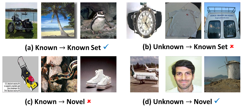
We evaluate our algorithm by using the features extracted from the pre-trained Alexnet [Krizhevsky et al.(2012)Krizhevsky, Sutskever, and Hinton] and VGG16 [Simonyan and Zisserman(2014)] networks as done in [Perera and Patel(2019)]. Our results are compared against the current state-of-the-art baseline methods and also evaluated on the same set of features and their results are directly taken from [Perera and Patel(2019)]. Our results as reported in Table 1 shows that our proposed model gives the best result in three out of four cases. Our method on VGG16 features has convincingly outperformed the method in [Perera and Patel(2019)] with a margin of 7.9 for Stanford Dogs [Khosla et al.(2011)Khosla, Jayadevaprakash, Yao, and Li] and 1.3 for Caltech 256 [Griffin et al.(2007)Griffin, Holub, and Perona] datasets. For Alexnet features, it beats all the other approaches for Stanford Dogs and compares favorably for Caltech 256 dataset. One important point to note is that our proposed framework does not require any external or auxiliary datasets as used in [Perera and Patel(2019)] to perform novelty detection. This makes our approach more suitable for real-world applications. Since it does not require any auxiliary dataset, it is also computationally lighter than [Perera and Patel(2019)] as we do not need to train any extra network module. We also display the novelty detection results on few test example images from the Caltech 256 dataset in Figure 4. We show successful (a,d) and failure (b,c) cases in Figure 4. Successful cases are the ones where a query known (or unknown) sample is classified to belong to the known (or novel) set.
5.3 Analysis and Observation
We perform extensive analysis to better understand the proposed framework and highlight the salient points.
Effect of number of top classes used for novelty computation:
During testing, we compare the query element with all individual class mean prototypes of the known set for determining whether it is novel or not.
The results are reported in Table 1 when the prototypes of all the known classes () are used during testing.
Here, we investigate the effect of taking the prototypes of only the top- classes (as given by the softmax values from the base network, namely Alexnet and VGG16) and provide the results in Figure 5.
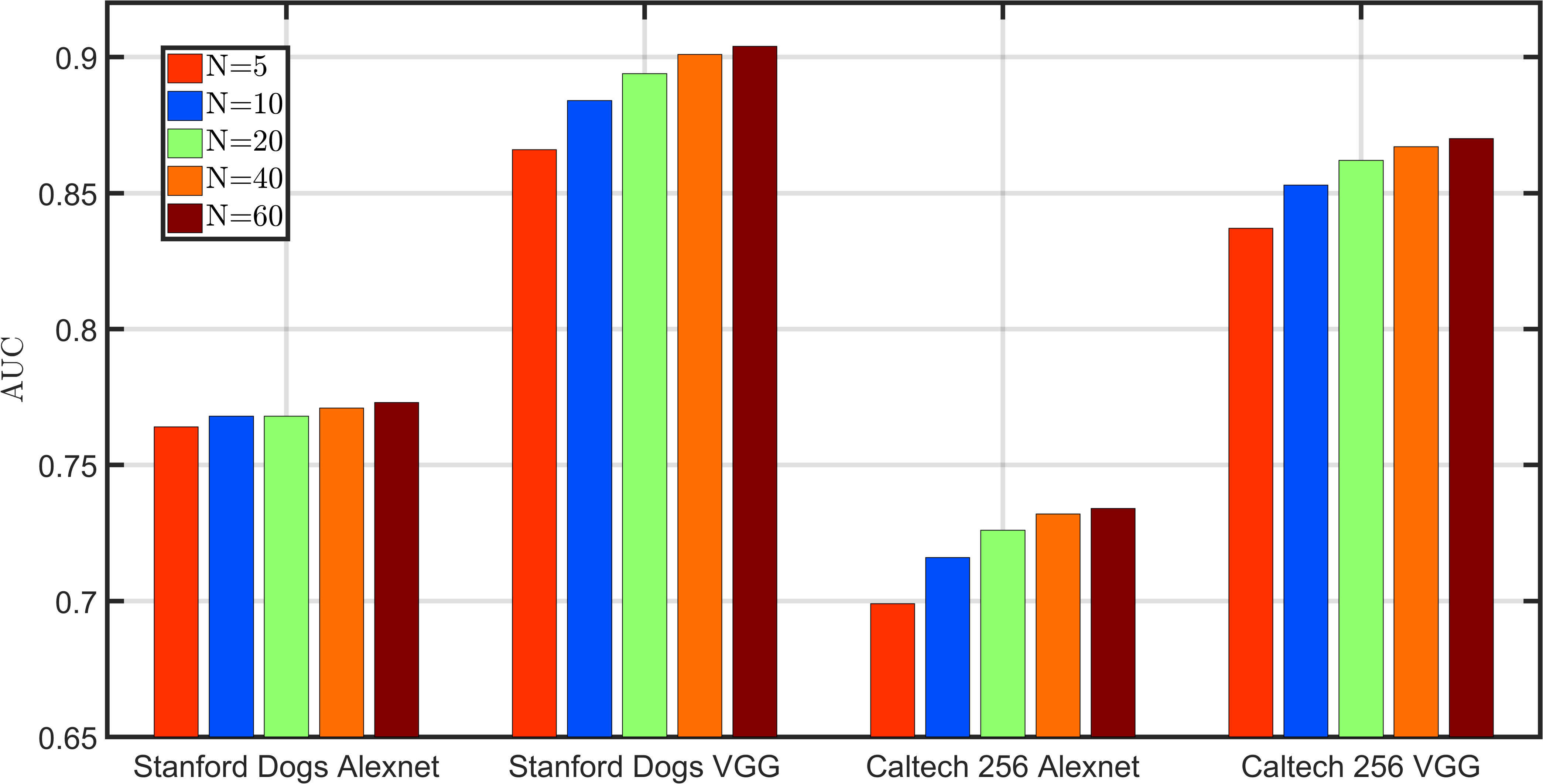
We observe that there is a very gradual monotonic decrease in the performance of our model as the value of is decreased from to .
This helps us to develop a computationally lighter version of our algorithm where we get satisfactory performance even when comparing the query with only the top few class prototypes.
This becomes especially useful when the number of known classes becomes very large.
Analysis of class-wise membership score:
To better understand why our model is working, we plot the average class-wise membership score for the images of the seen and unseen categories for the (a) Stanford Dogs (first categories as known) and (b) Caltech 256 dataset (first categories as known) in Figure 6.
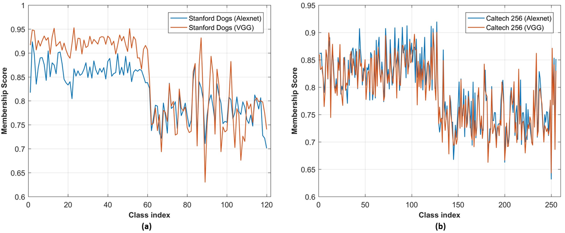
Two important conclusions can be drawn from here - (1) the difference in membership score between the seen and novel sets is more pronounced in case of the Stanford Dogs dataset than the Caltech 256 dataset.
This effectively means that our algorithm should perform better for the Stanford Dogs dataset which is further reflected in Table 1.
(2) The better performance of the VGG16 model over its Alexnet counterpart (as shown in Table 1) can be explained due to the fact that the membership profile for VGG16 has higher peaks and lower troughs than Alexnet.
A higher peak and lower trough leads to a better margin for error which results in more ease of determining whether a class is novel or not.
Varying the number of prototypes per class:
We have used the mean vector as the class prototype for each class in all our experiments.
We conduct experiments on the Stanford Dogs dataset to analyze here how the proposed framework performs when each known class is instead represented by a set of multiple feature vectors instead of a single mean vector.
The set of representative feature vectors for each class can be determined by applying k-means algorithm on each category and then selecting the subsequent cluster centers which have been formed.
| No of prototypes per class | ||||
|---|---|---|---|---|
| 1 | 2 | 3 | 5 | |
| VGG16 | 0.904 | 0.913 | 0.913 | 0.914 |
| AlexNet | 0.773 | 0.773 | 0.775 | 0.782 |
Performance in Table 2 show that there is a very slight increase in performance with the increase in the number of prototypes.
We thus select a single prototype to evaluate our model during the testing phase.
Effect of mixing coefficient :
Our model is trained by randomly sampling the value () and then assigning it to the pair of points.
The purpose of the network is to correctly predict the mixing coefficient.
During testing, we set to a fixed predefined value.
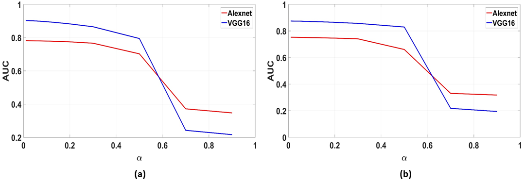
In Figure 7, we report the AUC performance of our model for different values of and observe that the value of the cluster center should be kept low to get better performance.
The reason for this being that, the interpolated point , formed by with, being the incoming query, and being the class prototype, is much closer to for a small value of .
Thus if and belong to the same class then the interpolated point should also belong to the same class leading to the trained model outputting a higher prediction value for that particular class.
Conversely, if belongs to a novel class altogether, the interpolated point should be far apart from leading the network to give a small value corresponding to that class.
Softmax vs Membership Scores: We analyze the Softmax score along with its membership value for few test cases in Figure 8 for the Stanford Dogs and Caltech 256 dataset respectively.
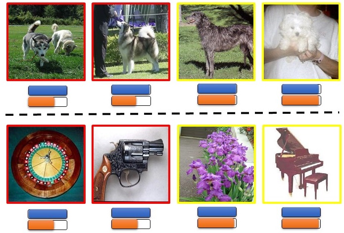
From the figure, it is clear that while the softmax values are overly confident signifying that the image possibly belongs to the known set, our membership score being low helps to determine that it is a novel sample.
Effect of loss weighting factor :
One of the critical design parameters of our algorithm is the choice of the hyper-parameter in equation (1).
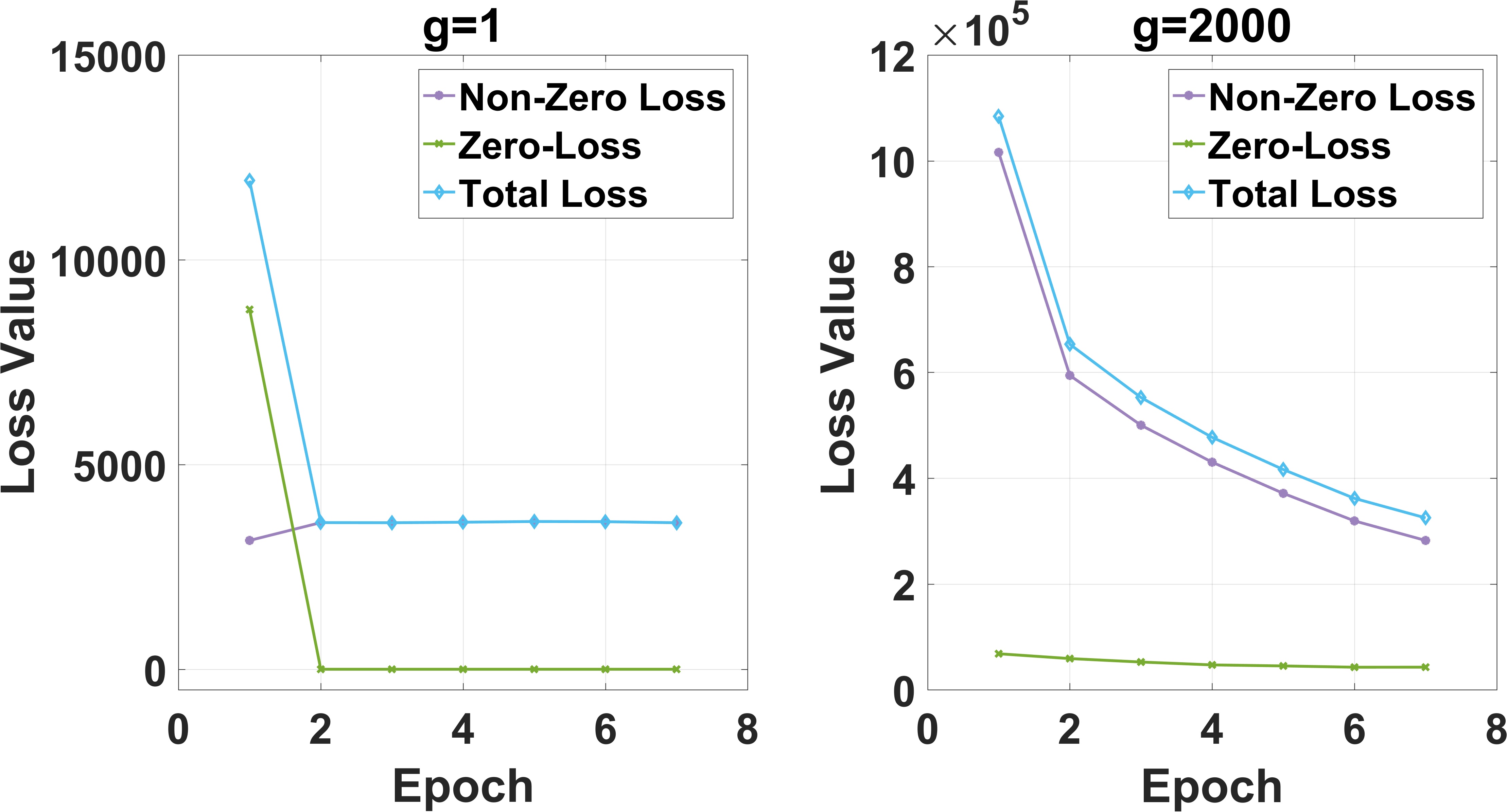
We observe from Figure 9 the training value loss profile for different values of for Stanford Dogs dataset when using the VGG16 features.
From the figure, we can draw the conclusion that having a weight of i.e., giving equal importance to the zero and non-zero loss gives poor result as the network only learns to output values close to zero.
A higher weight assigned to the non-zero element can help to effectively train our model as shown in Figure 9 thereby reducing both the losses.
6 Conclusions
In this paper, we have developed a novel methodology (MND) for multi-class novelty detection which works using the concept of mixup technique. We have designed a novel constituency loss for training our model. Experimental evaluations have shown that our model performs favorably with the current state-of-the-art even without having access to any extra auxiliary dataset. We have also developed an efficient version of our algorithm, without any significant drop in performance, which utilizes the softmax confidence outputs of the pre-trained network.
References
- [Abati et al.(2019)Abati, Porrello, Calderara, and Cucchiara] Davide Abati, Angelo Porrello, Simone Calderara, and Rita Cucchiara. Latent space autoregression for novelty detection. In IEEE Conference on Computer Vision and Pattern Recognition (CVPR), pages 481–490, 2019.
- [Akcay et al.(2018)Akcay, Atapour-Abarghouei, and Breckon] Samet Akcay, Amir Atapour-Abarghouei, and Toby P Breckon. Ganomaly: Semi-supervised anomaly detection via adversarial training. In Asian Conference on Computer Vision(ACCV), pages 622–637, 2018.
- [Bendale and Boult(2016)] Abhijit Bendale and Terrance E Boult. Towards open set deep networks. In IEEE Conference on Computer Vision and Pattern Recognition (CVPR), pages 1563–1572, 2016.
- [Bengio et al.(2013)Bengio, Mesnil, Dauphin, and Rifai] Yoshua Bengio, Grégoire Mesnil, Yann Dauphin, and Salah Rifai. Better mixing via deep representations. In International conference on machine learning (ICML), pages 552–560, 2013.
- [Berthelot et al.(2019)Berthelot, Raffel, Roy, and Goodfellow] David Berthelot, Colin Raffel, Aurko Roy, and Ian Goodfellow. Understanding and improving interpolation in autoencoders via an adversarial regularizer. In International Conference Learning Representations (ICLR), 2019.
- [Bodesheim et al.(2013)Bodesheim, Freytag, Rodner, Kemmler, and Denzler] Paul Bodesheim, Alexander Freytag, Erik Rodner, Michael Kemmler, and Joachim Denzler. Kernel null space methods for novelty detection. In IEEE Conference on Computer Vision and Pattern Recognition (CVPR), pages 3374–3381, 2013.
- [Bodesheim et al.(2015)Bodesheim, Freytag, Rodner, and Denzler] Paul Bodesheim, Alexander Freytag, Erik Rodner, and Joachim Denzler. Local novelty detection in multi-class recognition problems. In IEEE Winter Conference on Applications of Computer Vision (WACV), pages 813–820, 2015.
- [Bowman et al.(2015)Bowman, Vilnis, Vinyals, Dai, Jozefowicz, and Bengio] Samuel R Bowman, Luke Vilnis, Oriol Vinyals, Andrew M Dai, Rafal Jozefowicz, and Samy Bengio. Generating sentences from a continuous space. In SIGNLL Conference on Computational Natural Language Learning, pages 10–21, 2015.
- [Clifton et al.(2011)Clifton, Hugueny, and Tarassenko] David Andrew Clifton, Samuel Hugueny, and Lionel Tarassenko. Novelty detection with multivariate extreme value statistics. Journal of signal processing systems, 65(3):371–389, 2011.
- [Davis and Goadrich(2006)] Jesse Davis and Mark Goadrich. The relationship between precision-recall and roc curves. In International Conference on Machine learning(ICML), pages 233–240, 2006.
- [DeVries and Taylor(2018)] Terrance DeVries and Graham W Taylor. Learning confidence for out-of-distribution detection in neural networks. arXiv preprint arXiv:1802.04865, 2018.
- [Dumoulin et al.(2017)Dumoulin, Belghazi, Poole, Mastropietro, Lamb, Arjovsky, and Courville] Vincent Dumoulin, Ishmael Belghazi, Ben Poole, Olivier Mastropietro, Alex Lamb, Martin Arjovsky, and Aaron Courville. Adversarially learned inference. In International Conference Learning Representations (ICLR), 2017.
- [Eskin(2000)] Eleazar Eskin. Anomaly detection over noisy data using learned probability distributions. In International Conference on Machine Learning(ICML), pages 255–262, 2000.
- [Eskin et al.(2002)Eskin, Arnold, Prerau, Portnoy, and Stolfo] Eleazar Eskin, Andrew Arnold, Michael Prerau, Leonid Portnoy, and Sal Stolfo. A geometric framework for unsupervised anomaly detection. In Applications of data mining in computer security, pages 77–101. Springer, 2002.
- [Ge et al.(2017)Ge, Demyanov, Chen, and Garnavi] ZongYuan Ge, Sergey Demyanov, Zetao Chen, and Rahil Garnavi. Generative openmax for multi-class open set classification. In British Machine Vision Conference (BMVC), 2017.
- [Griffin et al.(2007)Griffin, Holub, and Perona] G. Griffin, A. Holub, and P. Perona. Caltech-256 object category dataset. Technical Report 7694, California Institute of Technology, 2007. URL http://authors.library.caltech.edu/7694.
- [Ha and Eck(2018)] David Ha and Douglas Eck. A neural representation of sketch drawings. In International Conference Learning Representations (ICLR), 2018.
- [Hautamaki et al.(2004)Hautamaki, Karkkainen, and Franti] Ville Hautamaki, Ismo Karkkainen, and Pasi Franti. Outlier detection using k-nearest neighbour graph. In International Conference on Pattern Recognition (ICPR), volume 3, pages 430–433, 2004.
- [Khosla et al.(2011)Khosla, Jayadevaprakash, Yao, and Li] Aditya Khosla, Nityananda Jayadevaprakash, Bangpeng Yao, and Fei-Fei Li. Novel dataset for fine-grained image categorization: Stanford dogs. In CVPR Workshop on Fine-Grained Visual Categorization (FGVC), volume 2, 2011.
- [Kim and Scott(2012)] JooSeuk Kim and Clayton D Scott. Robust kernel density estimation. Journal of Machine Learning Research, 13(Sep):2529–2565, 2012.
- [Knorr et al.(2000)Knorr, Ng, and Tucakov] Edwin M Knorr, Raymond T Ng, and Vladimir Tucakov. Distance-based outliers: algorithms and applications. The VLDB Journal—The International Journal on Very Large Data Bases, 8(3-4):237–253, 2000.
- [Krizhevsky et al.(2012)Krizhevsky, Sutskever, and Hinton] Alex Krizhevsky, Ilya Sutskever, and Geoffrey E Hinton. Imagenet classification with deep convolutional neural networks. In Advances in neural information processing systems (NIPS), pages 1097–1105, 2012.
- [Lee et al.(2018)Lee, Lee, Min, Zhang, Shin, and Lee] Kibok Lee, Kimin Lee, Kyle Min, Yuting Zhang, Jinwoo Shin, and Honglak Lee. Hierarchical novelty detection for visual object recognition. In IEEE Conference on Computer Vision and Pattern Recognition (CVPR), pages 1034–1042, 2018.
- [Liang et al.(2017)Liang, Li, and Srikant] Shiyu Liang, Yixuan Li, and R Srikant. Enhancing the reliability of out-of-distribution image detection in neural networks. arXiv preprint arXiv:1706.02690, 2017.
- [Liu et al.(2017)Liu, Lian, Wang, and Xiao] Juncheng Liu, Zhouhui Lian, Yi Wang, and Jianguo Xiao. Incremental kernel null space discriminant analysis for novelty detection. In IEEE Conference on Computer Vision and Pattern Recognition (CVPR), pages 792–800, 2017.
- [Markou and Singh(2003)] Markos Markou and Sameer Singh. Novelty detection: a review—part 1: statistical approaches. Signal processing, 83(12):2481–2497, 2003.
- [Masana et al.(2018)Masana, Ruiz, Serrat, van de Weijer, and Lopez] Marc Masana, Idoia Ruiz, Joan Serrat, Joost van de Weijer, and Antonio M Lopez. Metric learning for novelty and anomaly detection. In British Machine Vision Conference (BMVC), 2018.
- [Mathieu et al.(2016)Mathieu, Zhao, Zhao, Ramesh, Sprechmann, and LeCun] Michael F Mathieu, Junbo Jake Zhao, Junbo Zhao, Aditya Ramesh, Pablo Sprechmann, and Yann LeCun. Disentangling factors of variation in deep representation using adversarial training. In Advances in Neural Information Processing Systems(NIPS), pages 5040–5048, 2016.
- [Mescheder et al.(2017)Mescheder, Nowozin, and Geiger] Lars Mescheder, Sebastian Nowozin, and Andreas Geiger. Adversarial variational bayes: Unifying variational autoencoders and generative adversarial networks. In International Conference on Machine Learning(ICML), pages 2391–2400, 2017.
- [Mohammadi-Ghazi et al.(2018)Mohammadi-Ghazi, Marzouk, and Büyüköztürk] Reza Mohammadi-Ghazi, Youssef M Marzouk, and Oral Büyüköztürk. Conditional classifiers and boosted conditional gaussian mixture model for novelty detection. Pattern Recognition, 81:601–614, 2018.
- [Perera and Patel(2019)] Pramuditha Perera and Vishal M Patel. Deep transfer learning for multiple class novelty detection. In IEEE Conference on Computer Vision and Pattern Recognition(CVPR), pages 11544–11552, 2019.
- [Perera et al.(2019)Perera, Nallapati, and Xiang] Pramuditha Perera, Ramesh Nallapati, and Bing Xiang. Ocgan: One-class novelty detection using gans with constrained latent representations. In IEEE Conference on Computer Vision and Pattern Recognition (CVPR), pages 2898–2906, 2019.
- [Pidhorskyi et al.(2018)Pidhorskyi, Almohsen, and Doretto] Stanislav Pidhorskyi, Ranya Almohsen, and Gianfranco Doretto. Generative probabilistic novelty detection with adversarial autoencoders. In Advances in Neural Information Processing Systems(NIPS), pages 6822–6833, 2018.
- [Pimentel et al.(2014)Pimentel, Clifton, Clifton, and Tarassenko] Marco AF Pimentel, David A Clifton, Lei Clifton, and Lionel Tarassenko. A review of novelty detection. Signal Processing, 99:215–249, 2014.
- [Sabokrou et al.(2018)Sabokrou, Khalooei, Fathy, and Adeli] Mohammad Sabokrou, Mohammad Khalooei, Mahmood Fathy, and Ehsan Adeli. Adversarially learned one-class classifier for novelty detection. In IEEE Conference on Computer Vision and Pattern Recognition (CVPR), pages 3379–3388, 2018.
- [Sadooghi and Khadem(2018)] Mohammad Saleh Sadooghi and Siamak Esmaeilzadeh Khadem. Improving one class support vector machine novelty detection scheme using nonlinear features. Pattern Recognition, 83:14–33, 2018.
- [Schölkopf et al.(2001)Schölkopf, Platt, Shawe-Taylor, Smola, and Williamson] Bernhard Schölkopf, John C Platt, John Shawe-Taylor, Alex J Smola, and Robert C Williamson. Estimating the support of a high-dimensional distribution. Neural computation, 13(7):1443–1471, 2001.
- [Schultheiss et al.(2017)Schultheiss, Käding, Freytag, and Denzler] Alexander Schultheiss, Christoph Käding, Alexander Freytag, and Joachim Denzler. Finding the unknown: Novelty detection with extreme value signatures of deep neural activations. In German Conference on Pattern Recognition, pages 226–238. Springer, 2017.
- [Simonyan and Zisserman(2014)] Karen Simonyan and Andrew Zisserman. Very deep convolutional networks for large-scale image recognition. arXiv preprint arXiv:1409.1556, 2014.
- [Stevens(1984)] James P Stevens. Outliers and influential data points in regression analysis. Psychological Bulletin, 95(2):334, 1984.
- [Tokozume et al.(2017)Tokozume, Ushiku, and Harada] Yuji Tokozume, Yoshitaka Ushiku, and Tatsuya Harada. Learning from between-class examples for deep sound recognition. In International Conference Learning Representations (ICLR), 2017.
- [Tokozume et al.(2018)Tokozume, Ushiku, and Harada] Yuji Tokozume, Yoshitaka Ushiku, and Tatsuya Harada. Between-class learning for image classification. In IEEE Conference on Computer Vision and Pattern Recognition (CVPR), pages 5486–5494, 2018.
- [Vyas et al.(2018)Vyas, Jammalamadaka, Zhu, Das, Kaul, and Willke] Apoorv Vyas, Nataraj Jammalamadaka, Xia Zhu, Dipankar Das, Bharat Kaul, and Theodore L Willke. Out-of-distribution detection using an ensemble of self supervised leave-out classifiers. In European Conference on Computer Vision (ECCV), pages 550–564, 2018.
- [Yamanishi et al.(2004)Yamanishi, Takeuchi, Williams, and Milne] Kenji Yamanishi, Jun-Ichi Takeuchi, Graham Williams, and Peter Milne. On-line unsupervised outlier detection using finite mixtures with discounting learning algorithms. Data Mining and Knowledge Discovery, 8(3):275–300, 2004.
- [Zhang et al.(2018)Zhang, Cisse, Dauphin, and Lopez-Paz] Hongyi Zhang, Moustapha Cisse, Yann N Dauphin, and David Lopez-Paz. mixup: Beyond empirical risk minimization. In International Conference Learning Representations (ICLR), 2018.
- [Zong et al.(2018)Zong, Song, Min, Cheng, Lumezanu, Cho, and Chen] Bo Zong, Qi Song, Martin Renqiang Min, Wei Cheng, Cristian Lumezanu, Daeki Cho, and Haifeng Chen. Deep autoencoding gaussian mixture model for unsupervised anomaly detection. In International Conference Learning Representations (ICLR), 2018.