SCOPS: Self-Supervised Co-Part Segmentation

Abstract

Parts provide a good intermediate representation of objects that is robust with respect to the camera, pose and appearance variations. Existing works on part segmentation is dominated by supervised approaches that rely on large amounts of manual annotations and can not generalize to unseen object categories. We propose a self-supervised deep learning approach for part segmentation, where we devise several loss functions that aids in predicting part segments that are geometrically concentrated, robust to object variations and are also semantically consistent across different object instances. Extensive experiments on different types of image collections demonstrate that our approach can produce part segments that adhere to object boundaries and also more semantically consistent across object instances compared to existing self-supervised techniques.

1 Introduction

Much of the computer vision involves analyzing objects surrounding us, such as humans, cars, furniture, and so on. A major challenge in analyzing objects is to develop a model that is robust to the multitude of object transformations and deformations due to changes in camera pose, occlusions, object appearance, and pose variations. Parts provide a good intermediate representation of objects that is robust with respect to these variations. As a result, part-based representations are used in a wide range of object analysis tasks such as 3D reconstruction [55], detection [12], fine-grained recognition [25], pose estimation [20], etc.

Several types of 2D part representations have been used in the literature, with the three most common ones being landmarks, bounding boxes, and part segmentations. A common approach to the part analysis is to first manually annotate large amounts of data and then leverage fully-supervised approaches to recognize parts [9, 29, 2, 4, 5]. However, these annotations, especially part segmentation, are often quite costly. The annotations are also specific to a single object category and usually do not generalize to other object classes. Consequently, it is difficult to scale the fully-supervised models to unseen categories and there is a need for weakly supervised techniques for part recognition that only rely on very weak supervision or no supervision at all.

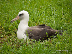
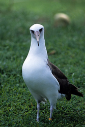
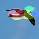
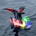
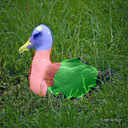
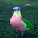
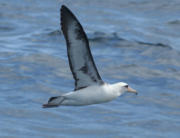
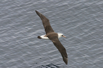
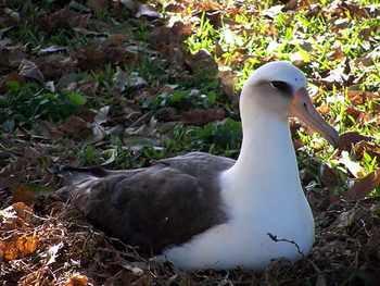
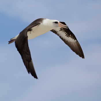
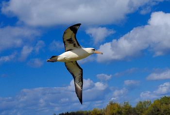
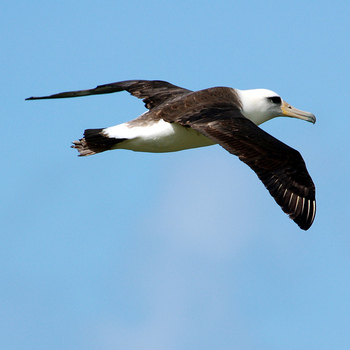
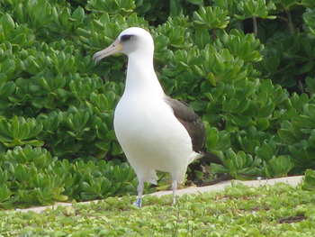
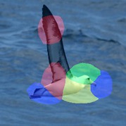
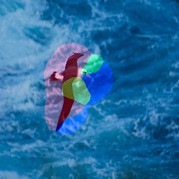
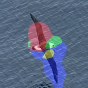
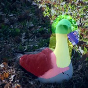
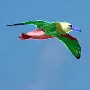
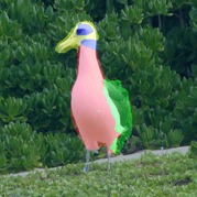
Part representations, once obtained, are robust to variations and help in high-level object understanding. However, obtaining part segmentations is challenging due to the above mentioned intra-class variations. An image collection of a single object category, despite having the same category objects, usually have high variability regarding pose, object appearances, camera viewpoint, the presence of multiple objects, etc. Figure 1 shows some sample images from three different image collections. Notice the variability across different object instances. Any weakly or unsupervised technique for part segmentation needs to reason about correspondences between different images which is challenging in such diverse image collections.

In this work, we propose a self-supervised deep learning framework for part segmentation. Given only an image collection of the same object category, our model can learn part segmentations that are semantically consistent across different object instances. Our learning technique is class agnostic, i.e., can be applied to any type of rigid or non-rigid object categories. And, we only use very weak supervision in the form of ImageNet pre-trained features [26, 39, 17], which are readily available. Contrary to recent deep learning techniques [42, 41, 50], which learn landmarks (keypoints) in a weakly or un-supervised manner, our network predicts part segmentation which provides much richer intermediate object representation compared to landmarks or bounding boxes.

To train our segmentation network, we consider several properties of a good part segmentation and encode that prior knowledge into the loss functions. Specifically, we consider four desirable characteristics of a part segmentation:

• Geometric concentration: Parts are concentrated geometrically and form connected components.

• Robustness to variations: Part segments are robust with respect to object deformations due to pose changes as well as camera and viewpoint changes.

• Semantic consistency: Part segments should be semantically consistent across different object instances with appearance and pose variations.

• Objects as union of parts: Parts appear on objects (not background) and the union of parts forms an object.

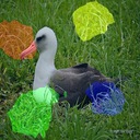
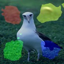
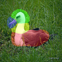
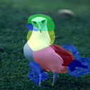
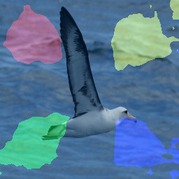
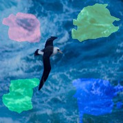
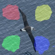
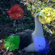
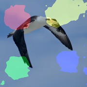
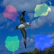
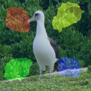
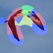
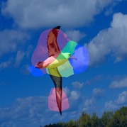
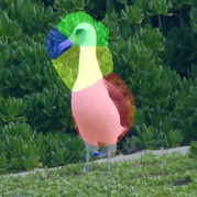
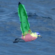
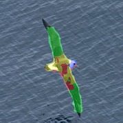
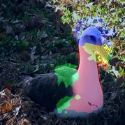
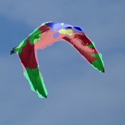
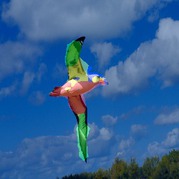
We devise loss functions that favor part segmentations that has above-mentioned qualities and use these loss functions to train our part segmentation network. We discuss these loss functions in detail in Section 3. We call our part segmentation network “SCOPS” (Self-Supervised Co-Part Segmentation). Figure 1 shows sample image collections and the corresponding part segmentations that SCOPS predicts. These visual results indicate that SCOPS can estimate part segmentations that are semantically consistent across object instances despite large variability across object instances.

When compared to recent unsupervised landmark detection approaches [42, 41, 50], our approach is relatively robust to appearance variations while also handling occlusions. Moreover, our approach can handle multiple object instances in an image which is not possible via landmark estimation with a fixed number of landmarks. When compared to the recent Deep Feature Factorization (DFF) approach [10], ours can scale to larger datasets, can produce sharper part segments that adhere to object boundaries and also more semantically consistent across object instances. We quantitatively evaluate our part segmentation results with an indirect measure of landmark estimation accuracy on unaligned CelebA [29], AFLW [22] and CUB [44] dataset images, and also with foreground segmentation accuracy on the PASCAL VOC dataset [11]. Results indicate that SCOPS consistently performs favorably against recent techniques. In summary, we propose a self-supervised deep network that can predict part segmentations that are semantically consistent across object instances while being relatively robust to object pose and appearance variations, camera variations and occlusions.

2 Related Works

Object concept discovery CNNs have shown impressive generalization capabilities across different computer vision tasks [45, 35, 1]. As a result, several works try to interpret and visualize the intermediate CNN representations  [49, 52, 3]. While some recent works [14, 3] demonstrate the presence of object part information in pre-trained CNN features, we aim to train a CNN that can predict consistent part segmentations in a self-supervised manner. Somewhat similar to our objective, class activation maps (CAMs) based methods [53, 34] propose to localize the dense response on image with respect to a trained classifier. However, without a learned part classifier, CAMs cannot be directly applied to our problem setting. Recently, Collins et al. [10] propose deep feature factorization (DFF) to estimate the common part segments in images through Non-negative Matrix Factorization (NMF) [27] on the ImageNet CNN features. However, DFF requires joint optimization during inference time, and it is costly to impose other constraints or loss functions on part maps since there is no standalone inference module. By posing as neural network inference, the proposed SCOPS can readily leverage the wealth of neural network loss functions developed in recent years. Any additional constraints can be jointly optimized during training time on large scale datasets, and the trained segmentation network could be applied on a single image during inference.

Landmark detection Recently, several techniques have been proposed to learn landmarks with weak or no supervision. Most of these works rely on geometric constrains and landmarks equivariance to transformations. Thewlis et al. [42] relied on geometric priors to learn landmarks that are invariant to affine and spline transformations. Zhang et al. [50] added reconstruction loss by reconstructing a given input image with predicted landmarks and local features. Honari et al. [18] used a subset of labeled images and sequential multitasking to improve final landmark estimation. Simon et al. [38] used multi-view bootstrapping to improve accuracy of hand landmark estimation. Suwajanakorn et al. [40] used multiple geometry aware losses to discover 3D landmarks. In order to obtain unsupervised landmarks, most of these works rely on simplified problem settings such as using cropped images with only a single object instance per image and allowing only minor occlusions. We aim to predict part segments which provide richer representation of objects compared to landmarks.

Dense image alignment Part segmentation is also related to the task of dense alignment, where the objective is to densely match pixels or landmarks from an object to another object instance. While conventional approaches utilize off-the-shelf feature descriptors matching to tackle the problem, e.g., SIFT flow based methods [28, 21, 6], recent works [16, 46, 47, 48, 15] utilize annotated landmark pairs and deep neural networks to learn a better feature descriptor or matching function. To avoid the cost of dense annotation, recent works propose to learn the dense alignment under the weakly supervised setting where only image pairs are required. Rocco et al. [30, 31] propose to jointly train the feature descriptor and spatial transformation by maximizing the inlier count, while Shu et al. [37] propose Deforming Autoencoder to align faces and disentangle expressions. However, these weakly supervised methods assume a certain family of spatial transforms, e.g., affine or thin plate spline grid, to align objects with similar poses. We argue that part segmentation is a more natural representation for semantic correspondences since matching each pixel between different instances would be an ill-posed problem. Part segmentations can also provide complex object deformations without heavily parameterized spatial transforms.

Image co-segmentation Co-segmentation approaches predict the foreground pixels of the specific object given an image collection. Most existing works [24, 32, 19, 43, 33] jointly consider all images within the collection to generate the final foreground segments via energy maximization, and thus not suitable for testing on standalone images. In contrast, we propose an end-to-end trainable network that takes single image as input and outputs part segmentation which is more challenging but provides more information compared to foreground segmentation.

Figure 2: SCOPS framework. Our network takes single image as input and predicts part segmentation. Geometric, Equivariance and Semantic Consistency constraints are used to train the network in a self-supervised manner.

3 Self-Supervised Co-Part Segmentation

Given an image collection of the same object category, we aim to learn a deep neural network that takes a single image as input and outputs part segmentations. As outlined in Section 1, we focus on the important characteristics of part segmentation and devise loss functions that endorse these properties: geometric concentration, robustness to variations, semantic consistency, and objects as the union of parts. Here, we first describe our overall framework followed by the description of different loss functions and how they encourage the above-mentioned properties. Along the way, we also comment on how our loss functions are related and different to existing loss functions in the literature.

3.1 Overall Framework

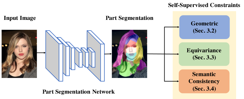
Figure 2 shows the overall framework of our proposed method. Given an image collection $\{\mathbf{I}\}$ of the same object category, we train a part segmentation network $\mathcal{F}$ parameterized by $\theta_{f}$, which is a fully convolutional neural network (FCN [36]) with a channel-wise softmax layer in the end, to generate the part response maps $\mathbf{R}=\mathcal{F}(\mathbf{I};\theta_{f})\in[0,1]^{(K+1)\times H\times W}$, where $K$ denotes the number of parts and $H\times W$ is the image resolution. Our network predicts $K+1$ channels with an additional channel indicating the background. To obtain the final part segmentation results, we first normalize each part map with it maximum response value in the spatial dimensions $\mathbf{\hat{R}}(k,i,j)=\mathbf{R}(k,i,j)/\max_{u,v}(\mathbf{R}(k,u,v))$, and we set the background map as constant with value $0.1$. The purpose of this normalization is to enhance weak part responses. Then the part segmentation is obtained with the $\arg\max$ function along the channel dimension. We use DeepLab-V2 [8] with ResNet50 [17] as our part segmentation network.

Since we do not assume the availability of any ground truth segmentation annotations, we formulate several constraints as differentiable loss functions to encourage the above mentioned desired properties of a part segmentation, such as geometry concentration and semantic consistency. The overall loss function for part segmentation network is a weighted sum of different loss functions which we describe next. Contrary to several co-segmentation approaches [24, 32, 19, 43, 33], which require multiple images during test-time inference, our network only takes a single image as input during the test time resulting in better portability of our trained model to unseen test images.

3.2 Geometric Concentration Loss

Pixels belonging to the same object part are usually spatially concentrated within an image and form a connected component unless there are occlusions or multiple instances. To this end, we first impose the geometric concentration on the part response maps to shape the part segments. Specifically, we utilize a loss term that encourages all the pixels belonging to a part to be spatially close to the part center. The part center for a part $k$ along axis $u$ is calculated as

$$c_{u}^{k}=\sum_{u,v}u\cdot\mathbf{R}(k,u,v)/z_{k},$$ (1)

where $z_{k}=\sum_{u,v}\mathbf{R}(k,u,v)$ is the normalization term to transform the part response map into a spatial probability distribution function. Then, we formulate the geometric concentration loss as

$$\mathcal{L}_{con}=\sum_{k}\sum_{u,v}||\langle u,v\rangle-\langle c_{u}^{k},c_{v}^{k}\rangle||^{2}\cdot\mathbf{R}(k,u,v)/z_{k},$$ (2)

and it is differentiable with respect to $c_{u}^{k}$, $\mathbf{R}(k,u,v)$, and $z_{k}$. This loss function encourages geometric concentration of parts and tries to minimize the variance of spatial probability distribution function $\mathbf{R}(k,u,v)/z_{k}$. This loss is closely related to ones used in recent unsupervised landmark estimation techniques [50, 42]. While Zhang et al. [50] approximate the landmark response maps with Gaussian distributions, we apply concentration loss mainly for penalizing part responses away from the part center.

Besides concentration loss, [50] and [42] propose a form of separation (diversity) loss that maximizes the distance between different landmarks. However, we do not employ such constraint as this constraint would results in separated part segments with background pixels in between.

Figure 3: Equivariance loss. We transform a given image with a random spatial transform and color jittering. We also transform the part segmentation of the given image using the same spatial transform to compare against the part segmentation of the transformed image via equivariance loss.

3.3 Equivariance Loss

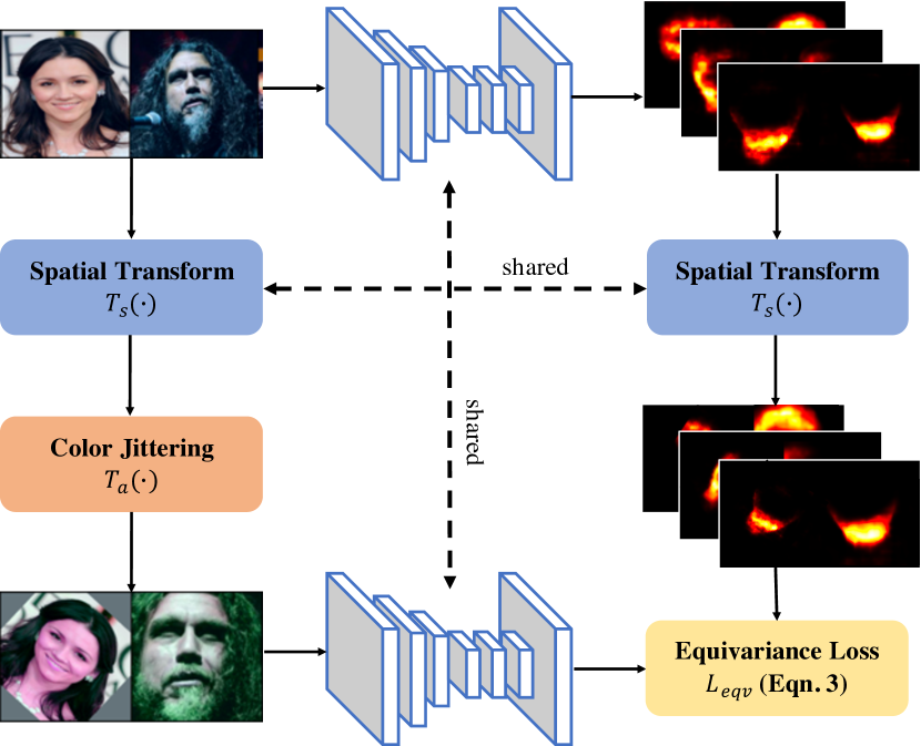
The second property that we want to advocate is that part segmentation should be robust to the appearance and pose variations. Figure 3 illustrates how we employ the equivariance constraints to encourage the robustness to variations. For each training image, we draw a random spatial transform $T_{s}(\cdot)$ and appearance perturbation $T_{a}(\cdot)$ from a predefined parameter range. The detailed transform parameters are present in the supplementary material. Then we pass both the input image $I$ and transformed image $I^{\prime}=T_{s}(T_{a}(I))$ through the segmentation network and obtain the corresponding response maps $\mathbf{R}$ and $\mathbf{R}^{\prime}$. Given these part response maps, we compute the part centers $\langle c_{u}^{k},c_{v}^{k}\rangle$ and $\langle c_{u}^{k^{\prime}},c_{v}^{k^{\prime}}\rangle$ using Eqn. 1. Then, the equivariance loss is defined as

$$\mathcal{L}_{eqv} =\lambda_{eqv}^{s}D_{KL}(\mathbf{R}^{\prime}||T_{s}(\mathbf{R}))$$

$$+\lambda_{eqv}^{c}\sum_{k}||\langle c_{u}^{k^{\prime}},c_{v}^{k^{\prime}}\rangle-T_{s}(\langle c_{u}^{k},c_{v}^{k}\rangle)||^{2},\vspace{-2mm}$$ (3)

where $D_{KL}(\cdot)$ is the Kullback–Leibler divergence distance, and $\lambda_{eqv}^{s},\lambda_{eqv}^{c}$ are the loss balancing coefficients. The first term corresponds to the part segmentation equivariance, and the second term denotes the part center equivariance. We use random similarity transformations (scale, rotation, and shifting) for spatial transforms. We also experimented with more complex transformations such as projective and thin-plate-spline transformations, but did not observe any improvements in part segmentation.

Recent works on unsupervised landmark estimation [50, 42] use the above-mentioned equivariance loss on landmarks (part centers). In this work, we extend the equivariance loss to part segmentation, and our experiments indicate that using only equivariance on part centers is not sufficient to obtain good part segmentation results.

3.4 Semantic Consistency Loss

Although equivariance loss favor part segmentations that are robust to some object variations, the synthetically created transformations would not be sufficient to produce consistency across different instances since the appearance and pose variations between images are too high to be modeled by any artificial transformations (See Figures 1 and 4 for some sample instances). To encourage semantic consistency across different object instances, we would need to explicitly leverage different instances in our loss function.

Figure 4: Semantic consistency loss. We enforce semantic consistency of parts across instances by learning a semantic part basis that is shared across all images. We use orthonormal constraint to learn distinct part basis, and we use saliency constraint to encourage parts to appear on foreground objects.

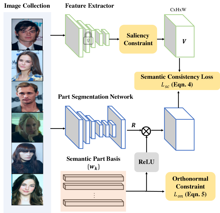
A key observation that we make use of is that the information about objects and parts is embedded in intermediate CNN features of classification networks  [3, 14, 10]. We devise a novel semantic consistency loss function that taps into this hidden part information of ImageNet trained features [26, 39, 17], which are readily available these days. Following the observation in [10], we assume that we can find representative feature clusters in the given classification features that are corresponding to different part segments.

Formally, given $C$-dimensional classification features $\mathbf{V}\in\mathcal{R}^{C\times H\times W}$, we like to find $K$ representative part features $\mathbf{w}_{k}\in\mathcal{R}^{C},k\in\{1,2,...,K\}$. We simultaneously learn part segmentation $\mathbf{R}$ and these representative part features $\{\mathbf{w}_{k}\}$ such that the classification features $\mathbf{V}(u,v)$ of an $(u,v)$ pixel belonging to $k^{th}$ part is close to $\mathbf{w}_{k}$ i.e., $||\mathbf{V}(u,v)-\mathbf{w}_{k}||^{2}\rightarrow 0$. Since the number of parts $K$ is usually smaller than feature dimensionality $C$, we can see the representative part features $\{\mathbf{w}_{k}\}$ as spanning a $K$-dimensional subspace in a $C$-dimensional space. We call these representative part features as part basis vectors.

Figure 4 illustrates the semantic consistency loss. Given an image $\mathbf{I}$, we obtain its part response map $\mathbf{R}$. We also pass $\mathbf{I}$ into a pre-trained classification network and obtain feature maps of an intermediate CNN layer. The feature map is bi-linearly up-sampled to have the same spatial resolution of $\mathbf{I}$ and $\mathbf{R}$, resulting in $\mathbf{V}\in\mathcal{R}^{C\times H\times W}$. We learn a set of part basis vectors $\{\mathbf{w}_{k}\}$ that are globally shared across different object instances (training images) using the following semantic consistency loss:

$$\vspace{-1mm}\mathcal{L}_{sc}=\sum_{u,v}||\mathbf{V}(u,v)-\sum_{k}\mathbf{R}(k,u,v)\mathbf{w}_{k}||^{2},\vspace{-1mm}$$ (4)

where $\mathbf{V}(u,v)\in\mathcal{R}^{C}$ is the feature vector sampled at spatial location $(u,v)$. We learn both the part segmentation $\mathbf{R}$ and the basis vectors $\{\mathbf{w}_{k}\}$ at the same time using standard back-propagation. To ensure that different part basis vectors do not cancel each other out, we enforce non-negativity on both features $\mathbf{V}$ and basis vectors $\{\mathbf{w}_{k}\}$ by passing them through a ReLU layer. The part segmentation $\mathbf{R}$ is naturally non-negative as it is the output of a softmax function.

We view the semantic consistency loss as a linear subspace recovery problem with respect to the embedding space provided by the feature extractor on the input image collection. As the training progresses, the part bases can gradually converge to the most representative direction of each part in the embedding space provided by the pre-trained deep features, and the recovered subspace can be described as the span of the basis $\{\mathbf{w}_{k}\}$. Furthermore, the non-negativity ensures that the weights $\mathbf{R}(k,u,v)$ could be interpreted as part responses. With the proposed semantic consistency loss, we explicitly enforce the cross-instance semantic consistency through the learned part basis $\{\mathbf{w}_{k}\}$ since the same part response would have similar semantic feature embedding in the pre-trained feature space.

Orthonormal Constraint When training with the semantic consistency loss, it is possible for the different basis to have similar feature embedding, especially when $K$ is large or the underlying rank of the subspace is smaller than $K$. Having similar part basis, the part segmentation could become noisy since the response from multiple channels could all represent the same part segment. Therefore, we propose to impose an additional orthonormal constraint on the part basis $\mathbf{w}_{k}$ to push the part bases apart. Let $\hat{\mathbf{W}}$ denotes the matrix with each row as a normalized part basis vector $\hat{\mathbf{w}_{k}}=\mathbf{w}_{k}/||\mathbf{w}_{k}||$, and we formulate the orthonormal constraint as a loss function on $W$:

$$\vspace{-1mm}\mathcal{L}_{on}=||\hat{\mathbf{W}}\hat{\mathbf{W}}^{T}-\mathbb{I}_{K}||_{F}^{2},\vspace{-1mm}$$ (5)

where $||\cdot||_{F}^{2}$ is Frobenius norm and $\mathbb{I}_{K}$ is the identity matrix of size $K\times K$. The idea is to minimize the correlation between different basis vectors, and thus we can obtain a more concise basis set resulting in better part responses.

Saliency Constraint We observe that, when the input image collection is small, or the number of parts $K$ is large, the proposed method tends to pick up some common background regions as object parts. To tackle this issue, we utilize an unsupervised saliency detection method [54] to suppress the background features in $\mathbf{V}$ so that the learned part basis do not correspond to background regions. To this end, for a given image and the unsupervised saliency map $\mathbf{D}\in[0,1]^{H\times W}$, we soft-mask the feature map $\mathbf{V}$ as $\mathbf{D}\circ\mathbf{V}$, where $\circ$ is the Hadamard (entry-wise) product, before passing it into the semantic consistency loss function. Considering the non-salient pixels where $\mathbf{D}(u,v)=0$, the semantic consistency loss (Eqn. 4) can be interpreted as solving the following equation:

$$\mathbf{R}(k,u,v)\mathbf{w}_{k}=0,\vspace{-1mm}$$ (6)

which is essentially projecting the non-salient background regions into the null space of the learned subspace spanned by $\{\mathbf{w}_{k}\}$. This saliency constraint encapsulates our prior knowledge that parts appear on objects (not background) and the union of parts forms an object. Several co-segmentation techniques [32, 7, 13] also make use of saliency maps to improve the segmentation result. However, to our best knowledge, we are the first work to impose the saliency constraint in the feature reconstruction loss.

Related to our semantic consistency loss, a recent work [10] proposed a deep feature factorization (DFF) technique for part discovery. Instead of learning a part basis, DFF proposes to directly factorize features $\mathbf{V}$ into response maps $\mathbf{R}$ and basis matrix $\mathbf{W}$ using non-negative matrix factorization (NMF); $\mathbf{V}\rightarrow\mathbf{R}\mathbf{W}$. Although DFF alleviates the need for learning a part basis and also training segmentation network, our learning strategy has several advantages compared to DFF. First, we can make use of mini-batches and standard gradient descent optimization techniques for learning part basis, whereas DFF performs NMF over the entire image collection at once during inference time. This makes our learning technique scalable to learning on large image collections and can be applied on single test image. Second, learning the part segmentation and basis using neural networks enables easy incorporation of different constraints on the part basis (e.g., orthonormal constraint) as well as the incorporation of other loss functions such as concentration and equivariance. Our experiments indicate that these loss functions are essential to obtain good part segmentations that are semantically consistent across images.

4 Experiments

Throughout the experiments, we refer to our technique as “SCOPS” (Self-supervised Co-Part Segmentation). Since SCOPS is self-supervised, the segmentation does not necessarily correspond to the human annotated object parts. Therefore, we quantitatively evaluate SCOPS with two different proxy measures on different object categories, including CelebA [29], AFLW [22] (human faces), CUB [44] (birds), and PASCAL [11] (common objects) datasets.

On CelebA, AFLW, and CUB datasets, we convert our part segmentation into landmarks by taking part centers (Eqn. 1) and evaluate against groundtruth annotations. Following recent works [50, 42], we fit a linear regressor that learns to map the detected landmarks to groundtruth landmarks and evaluate the resulting model on test data. On PASCAL, we aggregate the part segmentations and evaluate them with the foreground segmentation IOU.

Implementation Details We implement SCOPS with PyTorch, and we train the networks with a single Nvidia GPU. We use relu5_2 concatenated with relu5_4 from VGG-19 [39] as the pre-trained features $\mathbf{V}$ for the semantic consistency loss.

Table 1: Landmark evaluation on unaligned CelebA. Mean L2 distance comparing SCOPS to recent works (left) and also ablation with different loss functions (right).

Method	Error (%)
ULD (K=8) [50, 42]	40.82
DFF (K=8) [10]	31.30
SCOPS (K=4)	21.76
SCOPS (K=8)	15.01

SCOPS(K=8)	Error (%)
only $\mathcal{L}_{sc}$	23.53
w/o $\mathcal{L}_{sc}$	28.49
w/o $\mathcal{L}_{con}$	21.85
w/o $\mathcal{L}_{eqv}$	18.60
w/o Saliency	22.11

Table 2: Landmark evaluation on unaligned AFLW. Mean L2 distance comparing SCOPS to recent works.

Method	ULD (K=8) [50, 42]	DFF (K=8) [10]	SCOPS (K=8)
Error (%)	25.03	20.42	16.54

4.1 Faces from Unaligned CelebA/AFLW

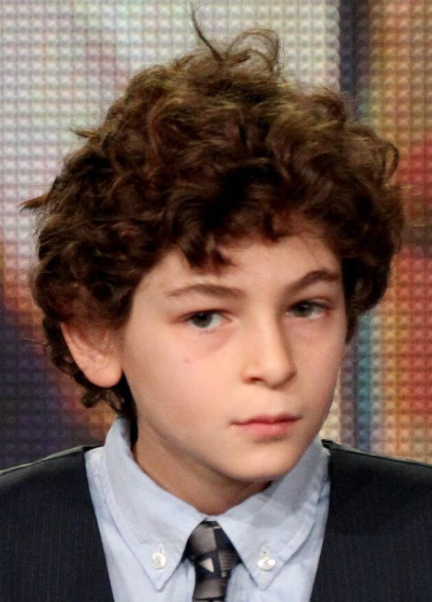
The CelebA dataset contains around 20k face images, each annotated with a tight bounding box around face and 5 facial landmarks. One of the main advantages of SCOPS is that it is relatively robust to pose and viewpoint variations compared to recent landmark estimation works [50, 42]. To demonstrate this, we experiment with unaligned CelebA images where we choose images with face covering more than 30% of the pixel area. Following the settings in [50], we also exclude MAFL [51] (subset of CelebA) test images from the train set resulting in a total of 45609 images. We use the MAFL train set (5379 images) to fit the linear regression model and test on the MAFL test set (283 images).

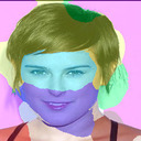
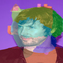
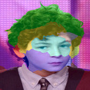
In Table 1, we report the landmark regression errors in terms of mean L2 distance normalized by inter-ocular distance. To compare with the existing unsupervised landmark discovery works, we implement the loss functions, including concentration, separation, landmark equivariance, and reconstruction, as proposed in [50] and [42]. We train our base network with these constraints and refer it as “ULD”. To validate our implementation of ULD, we train it on the align celebA images that yields 5.42% landmark estimation error, which is comparable to the reported 5.83% in [42] and 3.46% in [50]. However, when training and testing with the unaligned images, we found that ULD has difficulty in converging to semantically meaningful landmark locations, resulting in high errors. We also compare with a recent self-supervised part segmentation technique of DFF [10] by considering the part responses as landmark detections. We train SCOPS to predict 4 and 8 parts with all the proposed constraints and show the comparison results in Table 1 (left). The results show that SCOPS performs favorably against other methods. The visual results of SCOPS ($K=8$) in Fig. 5 shows that SCOPS part segments are more semantically consistent across different images compared to existing techniques. In addition, we train SCOPS on the AFLW dataset [22], which contains 4198 face images (after filtering) with 21 annotated landmarks. Following [50], we pretrain the model on CelebA and finetune on AFLW. We show the results in Table 2. Results indicate that SCOPS outperforms both ULD and DFF on this dataset images as well. Even though the landmark prediction accuracy do not directly measure the learned part segmentation quality, these results demonstrate that the learned part segmentations are semantically consistent across instances under the challenging unaligned setting.

image
ULD [50, 42]
DFF [10]
SCOPS
w/o $\mathcal{L}_{sc}$
only $\mathcal{L}_{sc}$
w/o $\mathcal{L}_{con}$
w/o $\mathcal{L}_{eqv}$
w/o saliency

Figure 5: Visual results on CelebA face images. SCOPS produce consistent part segments compared to existing techniques. Also shown is the effect of different loss constraints.

Ablation Study To validate the individual contribution of the different constraints, we conduct a detailed ablation study and show the results in Table 1 (right). The corresponding visual results are shown in Figure 5. While removing any of the constraints results in worse performance, the semantic consistency loss $\mathcal{L}_{sc}$ is the most important constraint in the proposed framework, and removing it would cause the most performance drop. Visual results in Figure 5 indicate that the learned parts would not have a semantic meaning without $\mathcal{L}_{sc}$. Results also indicate that training without geometric concentration loss $\mathcal{L}_{con}$ would cause some parts dominating large image areas, and no equivariance loss $\mathcal{L}_{eqv}$ makes the learned parts not consistent across images. These results demonstrate that all our loss functions are essential to learning good part segmentations.

Table 3: Landmark evaluation on CUB. Normalized L2 distance comparing SCOPS to recent techniques (K=4).

Method	CUB-001	CUB-002	CUB-003
ULD [50, 42]	30.12	29.36	28.19
DFF [10]	22.42	21.62	21.98
SCOPS	18.50	18.82	21.07

Image
ULD [50, 42]
DFF [10]
SCOPS

Figure 6: Visual results on CUB bird images. SCOPS is robust to pose and camera variations while having better boundary adherence compared to other techniques.

4.2 Birds from CUB

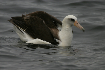
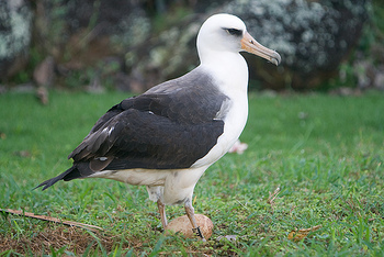
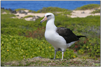
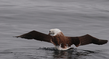
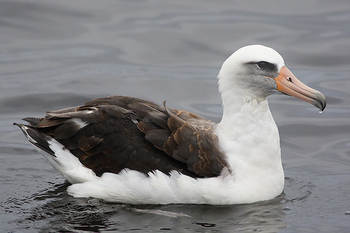
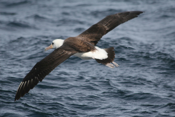
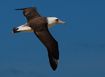
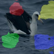
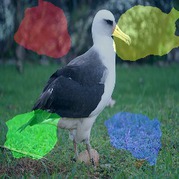
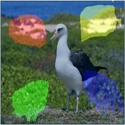
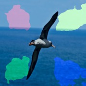
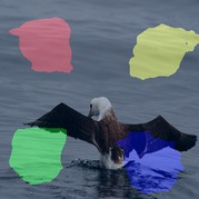
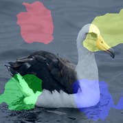
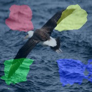
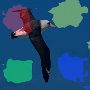
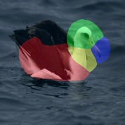
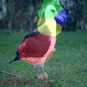
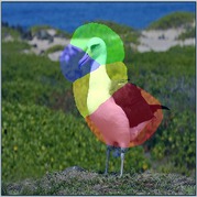
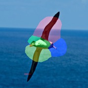
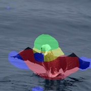
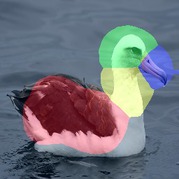
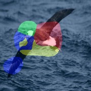
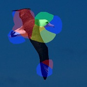
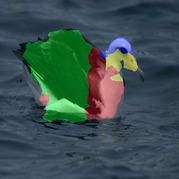
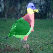
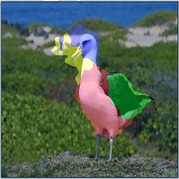
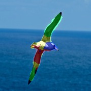
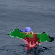
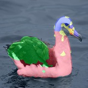
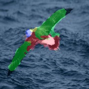
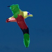
We also evaluate the proposed method on a more challenging bird images from CUB-2011 dataset [44], which consists of 11,788 images with 200 categories of birds and 15 landmark annotations. The dataset is challenging because of the various bird poses, e.g., standing, swimming, or flying, as well as the different camera viewpoints. We train SCOPS with $K=4$ on first three bird categories and compare to ULD and DFF. We show some qualitative results in Figure 19. With such level of object deformation, we found that ULD has difficulty in localizing meaningful parts. Compared to DFF, the part segments produced by SCOPS has better boundary alignment within and outside the object, and the learned part segmentation is also more consistent across instances. Similar to previous Section 4.1, we use the landmark detection as the proxy task through considering the part centers as detected landmarks. To account for the varying bird sizes across images, we normalize the landmark estimation error by the width and height of the provided ground truth bounding boxes. Table 3 shows the quantitative results of different techniques. For all the three bird categories, SCOPS performs favorably against both the ULD [50, 42], and DFF [10] techniques. For the CUB-2011 dataset, SCOPS as well as other techniques do not distinguish between left-right symmetric parts. For instance, the left-wing and right-wing are often predicted as the same part. From a part segmentation perspective, such behavior is reasonable. However, considering the landmark regression task, the part center of the two fanned out wings would be on the main body, resulting in less meaningful landmarks. As a result, the landmark regression error may not accurately reflect the co-part segmentation quality and distinguishing the symmetric semantic parts remains a challenging problem on this dataset images.

4.3 Common Objects from PASCAL

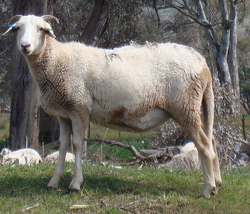
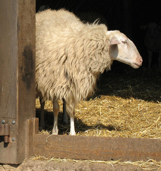
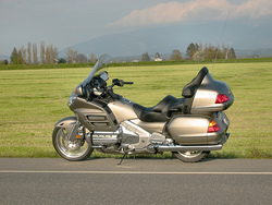
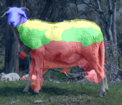
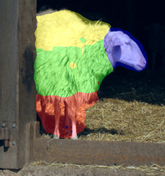
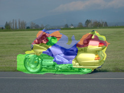
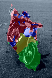
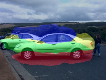
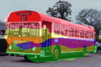
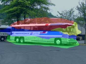
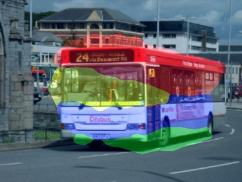
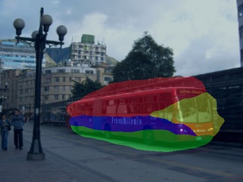
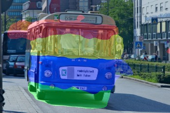
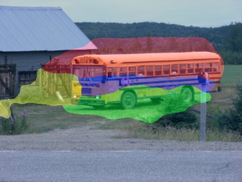
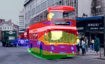
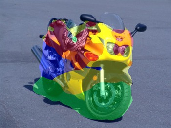
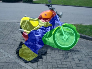
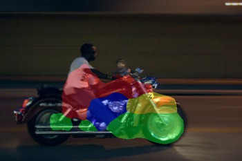
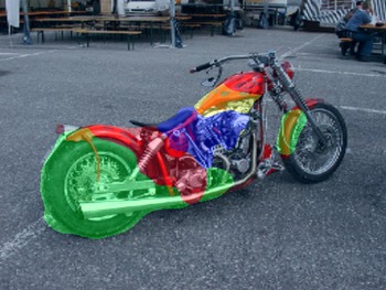
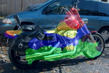
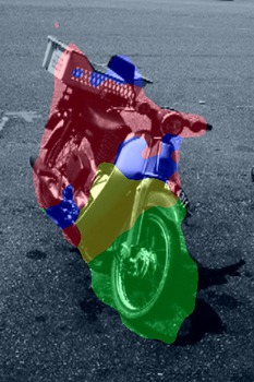
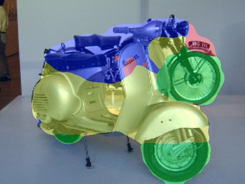
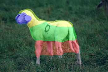
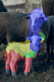
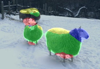
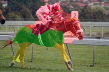
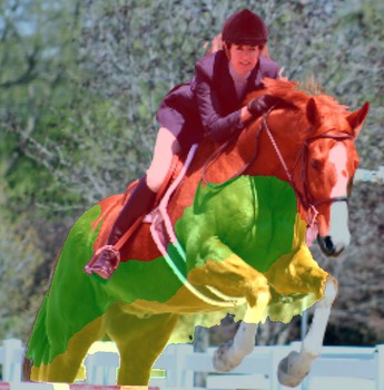
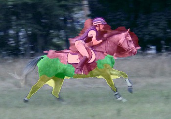
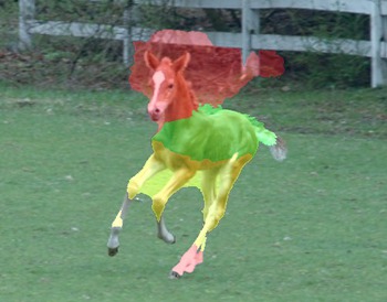
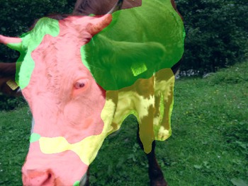
We also apply SCOPS on the PASCAL VOC dataset [11], which contains images with common objects with various deformations, viewing angles, and occlusions. We extract the images that contain the specific object category while the object bounding box occupies at least 20% of the whole image. To remove significant occlusions in the images, we further exclude the images where only a small portion of ground-truth parts are present in the PASCAL-part dataset [9]. The models are trained separately for each object category with $K=4$. Although the PASCAL-part dataset [9] provides the object parts annotation, a good self-supervised part segmentation can produce semantically consistent part segments that may not correspond to manually annotated part segments. Therefore, we do not evaluate the results with the part-level Intersection over Union (IoU) since it is not a good indicator. Instead, we evaluate the results as co-segmentation by aggregating the part segments and computing the foreground object segmentation IoU. Since the co-segmentation metric only indicates the overall object localization and not the part segmentation consistency, this metric is only indicative of part segmentation quality. We show some visual results in Figure 15 and the quantitative evaluations in Table 4. In terms of IoU, SCOPS outperform DFF by a considerable margin, both with and without the CRF post-processing [23]. The visual results show that SCOPS is robust to various appearance and pose articulations. We show additional visual results in the supplementary material.

Image
SCOPS

Figure 7: Visual results on the PASCAL VOC datset [11]. SCOPS is robust to pose and appearance variations.

Table 4: Evaluation on the PASCAL VOC dataset. Cosegmentation IoU comparing SCOPS to DFF on 7 object classes of VOC (K=4).

class	horse	cow	sheep	aero	bus	car	motor
DFF [10]	49.51	56.39	51.03	48.38	58.63	56.48	54.80
DFF+CRF [10]	50.96	57.64	52.29	50.87	58.64	57.56	55.86
SCOPS	55.76	60.79	56.95	69.02	73.82	65.18	58.53
SCOPS+CRF	57.92	62.70	58.17	80.54	75.32	66.14	59.15

5 Concluding Remarks

We propose SCOPS, a self-supervised technique for co-part segmentation. Given an image collection of an object category, SCOPS can learn to predict semantically consistent part segmentations without using any ground-truth annotations. We devise several constraints, including geometric concentration, equivariance, as well as semantic consistency, to train a deep neural network to discover semantically consistent part segments while ensuring decent geometric configurations and cross instance correspondence. Results on different types of image collections show that SCOPS is robust to different object appearances, camera viewpoints, as well as pose articulations. The qualitative and quantitative results show that SCOPS performs favorably against existing methods. We hope that the proposed method could serve as a general framework for learning co-part segmentation.

Acknowledgments.

W.-C. Hung is supported in part by the NSF CAREER Grant #1149783, gifts from Adobe, Verisk, and NEC.

Appendix A Optimization Objectives

In the proposed method, we train the part segmentation network and the semantic part basis with several loss functions, including geometric concentration loss $\mathcal{L}_{c}$, equivariance loss $\mathcal{L}_{eqv}$ and semantic consistency loss $\mathcal{L}_{sc}$, with orthonomal constraint $\mathcal{L}_{ot}$. The final objective function is a linear combination of these loss functions,

$$\mathcal{L}_{all}=\lambda_{c}\mathcal{L}_{c}+\lambda_{eqv}\mathcal{L}_{eqv}+\lambda_{sc}\mathcal{L}_{sc}+\lambda_{ot}\mathcal{L}_{ot}.$$ (7)

In all our experiments, the weighting coefficients $(\lambda_{c},\lambda_{eqv},\lambda_{sc},\lambda_{ot})$ are set to $(0.1,10,100,0.1)$. We obtain these weights by conducting a coarse grid search on a subset of the CelebA dataset images [29].

Appendix B Implementation Details of Equivariance Loss

For spatial transform, we apply random $\pm 60\degree$ rotation, $\pm 20\%$ shifting, $0.3x-2x$ scaling, as well as TPS transform with 5x5 grid and $\pm 10\%$ shifting for each control point. For color transform, we apply jittering to brightness ($\pm 30\%$), contrast ($\pm 30\%$), saturation ($\pm 20\%$), and hue ($\pm 20\%$). In our experiments, we find that the performance gain is robust with respect to a wide range of perturbation parameters.

Appendix C Additional Experimental Analysis

C.1 On Using Different Part Number $K$

We evaluate the effects of selected part number $K$ on the unaligned CelebA dataset [29]. We select $K=2,4,6,8,10$ and present the landmark estimation errors in Table 5. Note that with higher $K$ the landmarks’ center are more robust to face pose variations and thus lead to lower error rate. However, the performance seems to saturate after $K=8$. The qualitative results in Figure 8 also indicate the similar trend. When observing the part segmentation results for $K=8$ and $K=10$, the additional parts seem to be not corresponding to any semantically meaningful area of the face.

Table 5: Landmark evaluation on CelebA with different K. Mean L2 distance.

SCOPS	K = 2	K = 4	K = 6	K = 8	K = 10
Error (%)	25.46	21.76	15.92	15.01	14.71

C.2 Feature Visualization of Learned Semantic Part Basis

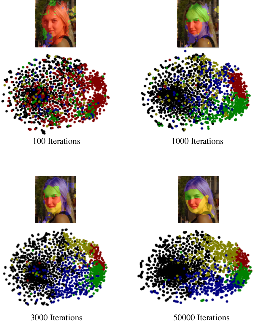
We also show how the learned part basis improves on training progress in Figure 9. The top images show the part segmentation results while the bottom show the t-SNE visualization [maaten2008visualizing] on the ImageNet feature of pixels and their corresponding segmentation class i.e., the dot colors correspond to the part segmentation visualization colors, while the black dots represent the background pixels. During the training process, we can see that the part segmentations are improving, while pixels with similar ImageNet features are segmented as same part.

Appendix D Quantitative Results on iCoseg

We present additional evaluation on the iCoseg dataset [batra2010icoseg], which is a commonly used co-segmentation dataset. Follow DFF [10], we select 5 image sets and train SCOPS with $K=4$ on the images. We aggregate the parts and evaluate with foreground segmentation IOU. The results show that SCOPS performs favorably against existing methods.

Table 6: Evaluation on iCoseg. Cosegmentation IoU comparing SCOPS to recent techniques on 5 image sets of iCoseg.

Subset	Elephants	Taj-Mahal	Pyramids	Gymnastics1	Statue of Liberty
Rubinstein [32]	63	48	57	94	70
DFF [10]	65	41	57	43	49
DFF-crf [10]	76	51	70	52	62
SCOPS	78.5	67.0	72.7	73.5	63.8
SCOPS-crf	81.5	66.0	75.0	81.5	65.7

Appendix E Qualitative Results on PASCAL Objects

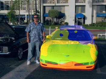
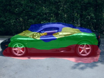
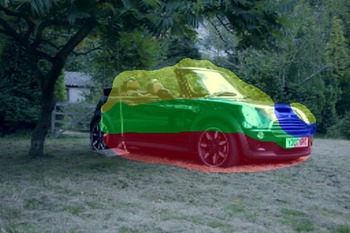
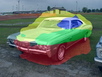
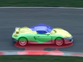
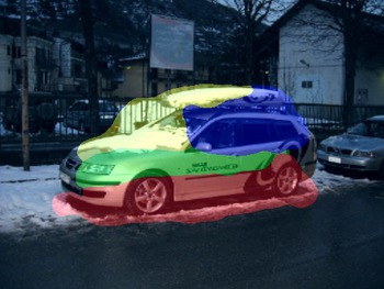
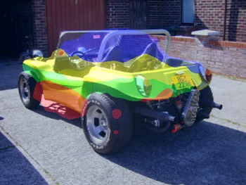
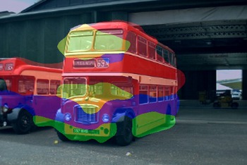
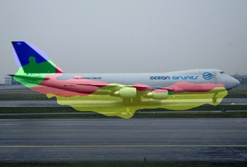
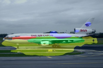
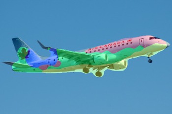
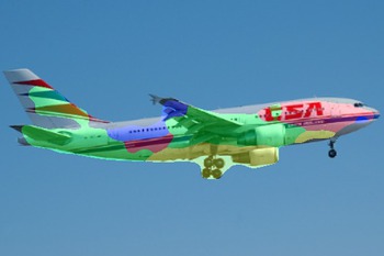
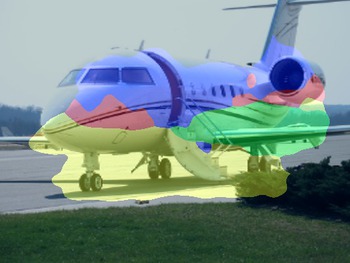
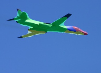
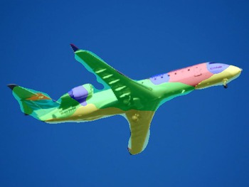
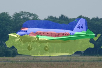
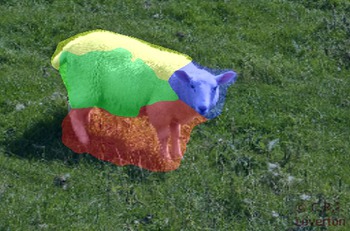
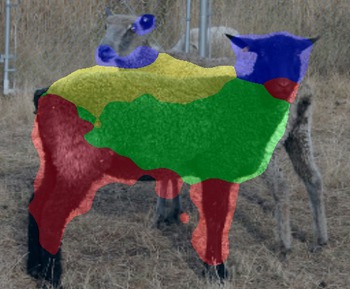
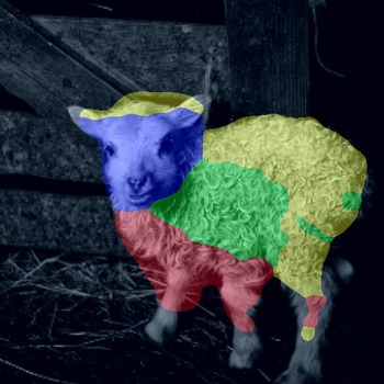
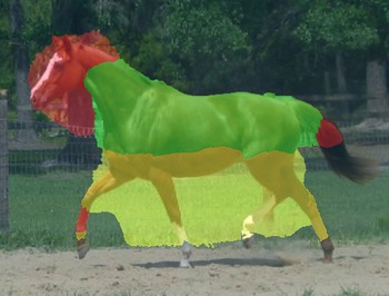
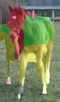
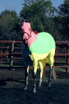
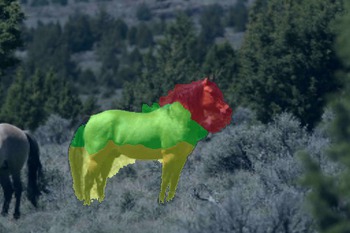
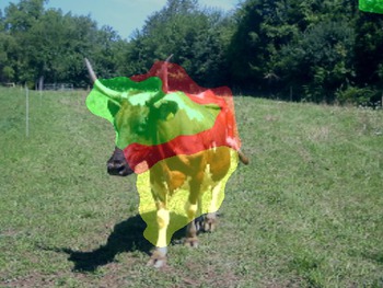
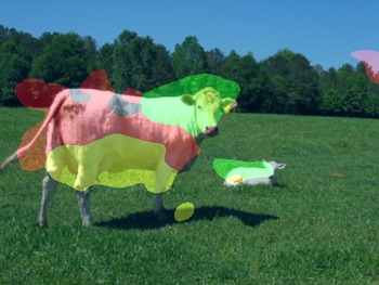
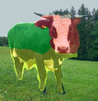
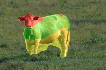
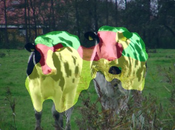
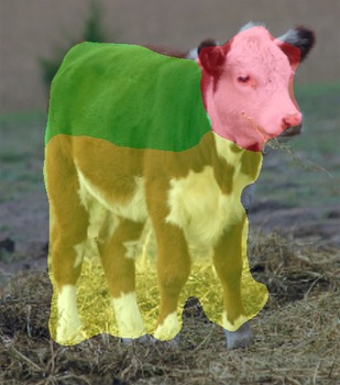
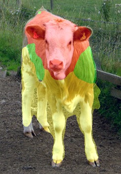
We present additional part segmentation visual results on different object class images obtained from the PASCAL dataset [11]. In Figures 10-16, the results show that the proposed method works for both rigid (Figures 10-13) and non-rigid (Figures 14-16) objects, where SCOPS produce part segments that are consistent across different instances with variations in appearance, pose and camera viewpoints.

Appendix F Additional Results on Unaligned CelebA and CUB

We provide more visual results on the unaligned CelebA dataset [29] and the CUB dataset [44] in Figures 17-20. The results show that SCOPS is robust to pose and camera variations while having better boundary adherence compared to other techniques.

Image
Saliency
SCOPS (K=2)
SCOPS (K=4)
SCOPS (K=6)
SCOPS (K=8)
SCOPS (K=10)

Figure 8: Effects of changing part number. We apply SCOPS on the unaligned CelebA dataset with the part number K ranging from 2 to 10.

Figure 9: Training progression. The top images show the part segmentation results while the bottom show the TSNE visualization on the imagenet feature of pixels and their corresponding segmentation class. Black dots are the background pixels. During the training process, we can see that the part segmentations are improving, while pixels with similar imagenet features are segmented as same part.

Image
SCOPS (K=4)

Figure 10: SCOPS visual results on car class images in the PASCAL dataset.

Image
SCOPS (K=4)

Figure 11: SCOPS visual results on bus class images in the PASCAL dataset.

Image
SCOPS (K=4)

Figure 12: SCOPS visual results on aeroplane class images in the PASCAL dataset.

Image
SCOPS (K=4)

Figure 13: SCOPS visual results on motor class images in the PASCAL dataset.

Image
SCOPS (K=4)

Figure 14: SCOPS visual results on sheep class images in the PASCAL dataset.

Image
SCOPS (K=3)

Figure 15: SCOPS visual results on horse class images in the PASCAL dataset.

Image
SCOPS (K=3)

Figure 16: SCOPS visual results on cow class images in the PASCAL dataset.

Image
Saliency
ULD [50, 42]
DFF [10]
SCOPS
w/o $\mathcal{L}_{sc}$
only $\mathcal{L}_{sc}$
w/o $\mathcal{L}_{con}$
w/o $\mathcal{L}_{eqv}$
w/o saliency

Figure 17: Additional visual results on CelebA face images. SCOPS produce consistent part segments compared to existing techniques. Also shown is the effect of different loss constraints.

Image
Saliency
ULD [50, 42]
DFF [10]
SCOPS
w/o $\mathcal{L}_{sc}$
only $\mathcal{L}_{sc}$
w/o $\mathcal{L}_{con}$
w/o $\mathcal{L}_{eqv}$
w/o saliency

Figure 18: Additional visual results on CelebA face images. SCOPS produce consistent part segments compared to existing techniques. Also shown is the effect of different loss constraints.

Image
ULD [50, 42]
DFF [10]
SCOPS

Figure 19: Additional visual results on CUB bird images. SCOPS is robust to pose and camera variations while having better boundary adherence compared to other techniques.

Image
ULD [50, 42]
DFF [10]
SCOPS

Figure 20: Additional visual results on CUB bird images. SCOPS is robust to pose and camera variations while having better boundary adherence compared to other techniques.

References

- [1] Pulkit Agrawal, Ross Girshick, and Jitendra Malik. Analyzing the performance of multilayer neural networks for object recognition. In ECCV. Springer, 2014.
- [2] Hossein Azizpour and Ivan Laptev. Object detection using strongly-supervised deformable part models. In ECCV. Springer, 2012.
- [3] David Bau, Bolei Zhou, Aditya Khosla, Aude Oliva, and Antonio Torralba. Network dissection: Quantifying interpretability of deep visual representations. In CVPR, 2017.
- [4] Lubomir Bourdev and Jitendra Malik. Poselets: Body part detectors trained using 3d human pose annotations. In ICCV. IEEE, 2009.
- [5] Steve Branson, Pietro Perona, and Serge Belongie. Strong supervision from weak annotation: Interactive training of deformable part models. In ICCV. IEEE, 2011.
- [6] Hilton Bristow, Jack Valmadre, and Simon Lucey. Dense semantic correspondence where every pixel is a classifier. In ICCV, 2015.
- [7] Kai-Yueh Chang, Tyng-Luh Liu, and Shang-Hong Lai. From co-saliency to co-segmentation: An efficient and fully unsupervised energy minimization model. In CVPR, 2011.
- [8] Liang-Chieh Chen, George Papandreou, Iasonas Kokkinos, Kevin Murphy, and Alan L Yuille. Deeplab: Semantic image segmentation with deep convolutional nets, atrous convolution, and fully connected crfs. In TPAMI, 2017.
- [9] Xianjie Chen, Roozbeh Mottaghi, Xiaobai Liu, Sanja Fidler, Raquel Urtasun, and Alan Yuille. Detect what you can: Detecting and representing objects using holistic models and body parts. In CVPR, 2014.
- [10] Edo Collins, Radhakrishna Achanta, and Sabine Süsstrunk. Deep feature factorization for concept discovery. In ECCV, 2018.
- [11] Mark Everingham, Luc J. Van Gool, Christopher K. I. Williams, John M. Winn, and Andrew Zisserman. The pascal visual object classes (voc) challenge. IJCV, 88(2):303–338, 2010.
- [12] Pedro Felzenszwalb, David McAllester, and Deva Ramanan. A discriminatively trained, multiscale, deformable part model. In CVPR, 2008.
- [13] Huazhu Fu, Dong Xu, Stephen Lin, and Jiang Liu. Object-based rgbd image co-segmentation with mutex constraint. In CVPR, 2015.
- [14] Abel Gonzalez-Garcia, Davide Modolo, and Vittorio Ferrari. Do semantic parts emerge in convolutional neural networks? IJCV, 2018.
- [15] Bumsub Ham, Minsu Cho, Cordelia Schmid, and Jean Ponce. Proposal flow. In CVPR, 2016.
- [16] Kai Han, Rafael S Rezende, Bumsub Ham, Kwan-Yee K Wong, Minsu Cho, Cordelia Schmid, and Jean Ponce. Scnet: Learning semantic correspondence. In ICCV, 2017.
- [17] Kaiming He, Xiangyu Zhang, Shaoqing Ren, and Jian Sun. Deep residual learning for image recognition. In CVPR, 2016.
- [18] Sina Honari, Pavlo Molchanov, Stephen Tyree, Pascal Vincent, Christopher Pal, and Jan Kautz. Improving landmark localization with semi-supervised learning. In CVPR, 2018.
- [19] Armand Joulin, Francis Bach, and Jean Ponce. Multi-class cosegmentation. In CVPR, 2012.
- [20] Martin Kiefel and Peter Vincent Gehler. Human pose estimation with fields of parts. In ECCV, 2014.
- [21] Jaechul Kim, Ce Liu, Fei Sha, and Kristen Grauman. Deformable spatial pyramid matching for fast dense correspondences. In CVPR, 2013.
- [22] Martin Koestinger, Paul Wohlhart, Peter M Roth, and Horst Bischof. Annotated facial landmarks in the wild: A large-scale, real-world database for facial landmark localization. In ICCV workshops, 2011.
- [23] Philipp Krähenbühl and Vladlen Koltun. Efficient inference in fully connected crfs with gaussian edge potentials. In Advances in neural information processing systems, pages 109–117, 2011.
- [24] Jonathan Krause, Hailin Jin, Jianchao Yang, and Li Fei-Fei. Fine-grained recognition without part annotations. In CVPR, 2015.
- [25] Jonathan Krause, Michael Stark, Jia Deng, and Li Fei-Fei. 3d object representations for fine-grained categorization. In Proceedings of the IEEE International Conference on Computer Vision Workshops, 2013.
- [26] A. Krizhevsky, I. Sutskever, and G. E. Hinton. Imagenet classification with deep convolutional neural networks. In NIPS, 2012.
- [27] Daniel D Lee and H Sebastian Seung. Learning the parts of objects by non-negative matrix factorization. Nature, 401(6755):788, 1999.
- [28] Ce Liu, Jenny Yuen, and Antonio Torralba. Sift flow: Dense correspondence across scenes and its applications. IEEE Transactions on Pattern Analysis and Machine Intelligence, 2011.
- [29] Ziwei Liu, Ping Luo, Xiaogang Wang, and Xiaoou Tang. Deep learning face attributes in the wild. In ICCV, 2015.
- [30] Ignacio Rocco, Relja Arandjelovic, and Josef Sivic. Convolutional neural network architecture for geometric matching. In CVPR, volume 2, 2017.
- [31] Ignacio Rocco, Relja Arandjelovic, and Josef Sivic. End-to-end weakly-supervised semantic alignment. In CVPR, 2018.
- [32] Michael Rubinstein, Armand Joulin, Johannes Kopf, and Ce Liu. Unsupervised joint object discovery and segmentation in internet images. In CVPR, 2013.
- [33] Jose C Rubio, Joan Serrat, Antonio López, and Nikos Paragios. Unsupervised co-segmentation through region matching. In CVPR, 2012.
- [34] Ramprasaath R Selvaraju, Michael Cogswell, Abhishek Das, Ramakrishna Vedantam, Devi Parikh, Dhruv Batra, et al. Grad-cam: Visual explanations from deep networks via gradient-based localization. In ICCV, 2017.
- [35] Ali Sharif Razavian, Hossein Azizpour, Josephine Sullivan, and Stefan Carlsson. Cnn features off-the-shelf: an astounding baseline for recognition. In CVPR Workshop, 2014.
- [36] Jonathan Shelhamer, Evan an Long and Trevor Darrell. Fully convolutional networks for semantic segmentation. TPAMI, 2016.
- [37] Zhixin Shu, Mihir Sahasrabudhe, Alp Guler, Dimitris Samaras, Nikos Paragios, and Iasonas Kokkinos. Deforming autoencoders: Unsupervised disentangling of shape and appearance. ECCV, 2018.
- [38] Tomas Simon, Hanbyul Joo, Iain A Matthews, and Yaser Sheikh. Hand keypoint detection in single images using multiview bootstrapping. In CVPR, 2017.
- [39] Karen Simonyan and Andrew Zisserman. Very deep convolutional networks for large-scale image recognition. In ICLR, 2015.
- [40] Supasorn Suwajanakorn, Noah Snavely, Jonathan Tompson, and Mohammad Norouzi. Discovery of latent 3d keypoints via end-to-end geometric reasoning. arXiv preprint arXiv:1807.03146, 2018.
- [41] James Thewlis, Hakan Bilen, and Andrea Vedaldi. Unsupervised learning of object frames by dense equivariant image labelling. In NIPS, 2017.
- [42] James Thewlis, Hakan Bilen, and Andrea Vedaldi. Unsupervised learning of object landmarks by factorized spatial embeddings. In ICCV, 2017.
- [43] Yi-Hsuan Tsai, Guangyu Zhong, and Ming-Hsuan Yang. Semantic co-segmentation in videos. In ECCV, 2016.
- [44] Catherine Wah, Steve Branson, Peter Welinder, Pietro Perona, and Serge Belongie. The caltech-ucsd birds-200-2011 dataset. 2011.
- [45] Jason Yosinski, Jeff Clune, Yoshua Bengio, and Hod Lipson. How transferable are features in deep neural networks? In NIPS, 2014.
- [46] Sergey Zagoruyko and Nikos Komodakis. Learning to compare image patches via convolutional neural networks. In CVPR, 2015.
- [47] Jure Zbontar and Yann LeCun. Computing the stereo matching cost with a convolutional neural network. In CVPR, 2015.
- [48] Jure Zbontar and Yann LeCun. Stereo matching by training a convolutional neural network to compare image patches. Journal of Machine Learning Research, 2016.
- [49] Matthew D Zeiler and Rob Fergus. Visualizing and understanding convolutional networks. In ECCV. Springer, 2014.
- [50] Yuting Zhang, Yijie Guo, Yixin Jin, Yijun Luo, Zhiyuan He, and Honglak Lee. Unsupervised discovery of object landmarks as structural representations. In CVPR, 2018.
- [51] Zhanpeng Zhang, Ping Luo, Chen Change Loy, and Xiaoou Tang. Facial landmark detection by deep multi-task learning. In ECCV. Springer, 2014.
- [52] Bolei Zhou, Aditya Khosla, Agata Lapedriza, Aude Oliva, and Antonio Torralba. Object detectors emerge in deep scene cnns. In ICLR, 2015.
- [53] Bolei Zhou, Aditya Khosla, Agata Lapedriza, Aude Oliva, and Antonio Torralba. Learning deep features for discriminative localization. In CVPR, 2016.
- [54] Wangjiang Zhu, Shuang Liang, Yichen Wei, and Jian Sun. Saliency optimization from robust background detection. In CVPR, 2014.
- [55] Silvia Zuffi and Michael J Black. The stitched puppet: A graphical model of 3d human shape and pose. In CVPR, 2015.