PRECOG: PREdiction Conditioned On Goals in Visual Multi-Agent Settings

Nicholas Rhinehart1
   Rowan McAllister2
   Kris Kitani1
   Sergey Levine2
   1Carnegie Mellon University
{nrhineha,kkitani}@cs.cmu.edu
   2University of California, Berkeley
{rmcallister,svlevine}@berkeley.edu
Abstract

For autonomous vehicles (AVs) to behave appropriately on roads populated by human-driven vehicles, they must be able to reason about the uncertain intentions and decisions of other drivers from rich perceptual information. Towards these capabilities, we present a probabilistic forecasting model of future interactions between a variable number of agents. We perform both standard forecasting and the novel task of conditional forecasting, which reasons about how all agents will likely respond to the goal of a controlled agent (here, the AV). We train models on real and simulated data to forecast vehicle trajectories given past positions and LIDAR. Our evaluation shows that our model is substantially more accurate in multi-agent driving scenarios compared to existing state-of-the-art. Beyond its general ability to perform conditional forecasting queries, we show that our model’s predictions of all agents improve when conditioned on knowledge of the AV’s goal, further illustrating its capability to model agent interactions.

1 Introduction

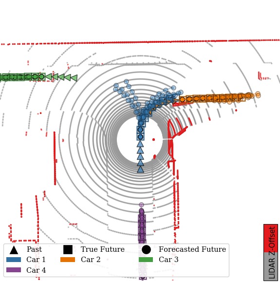
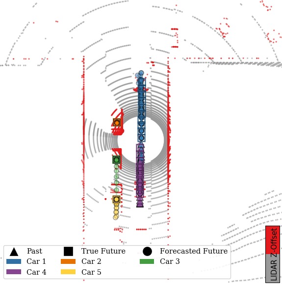
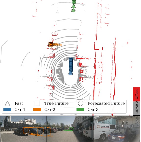
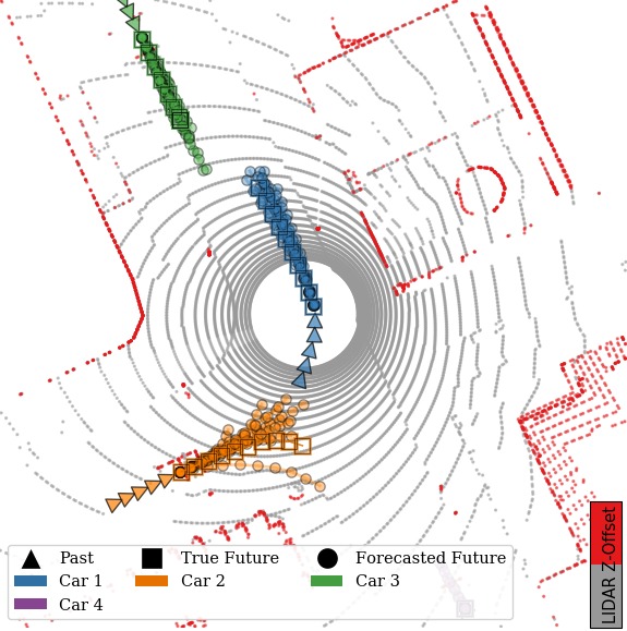
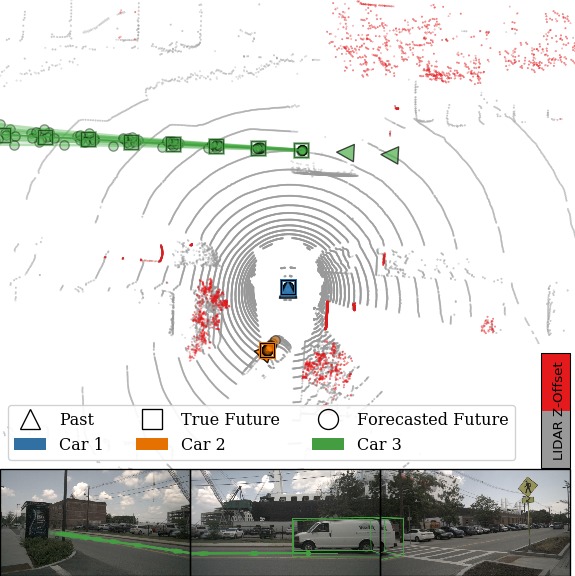
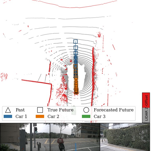
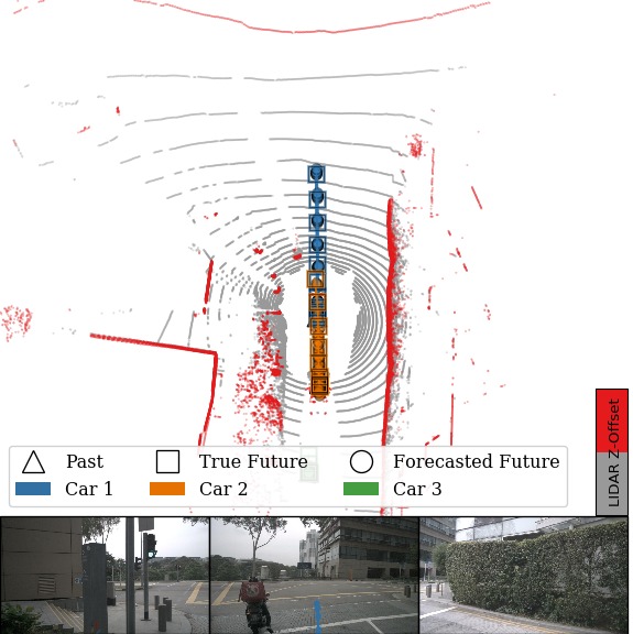
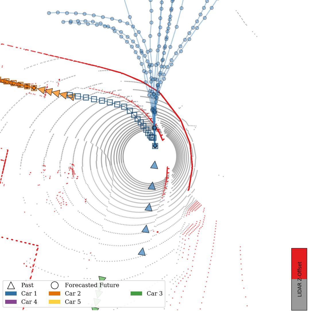
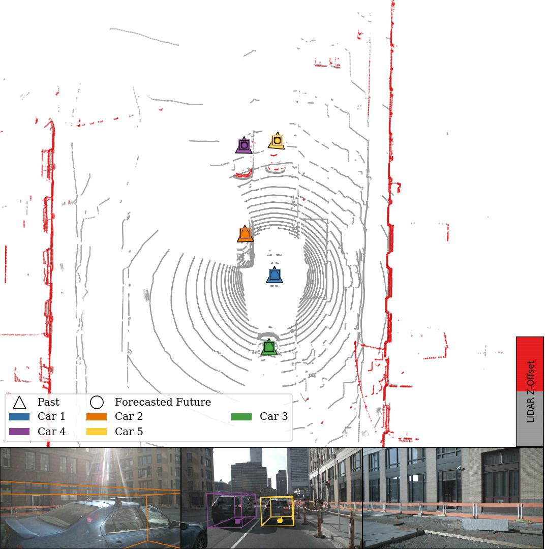
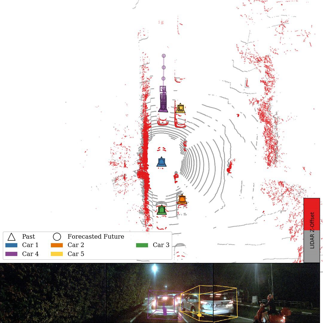
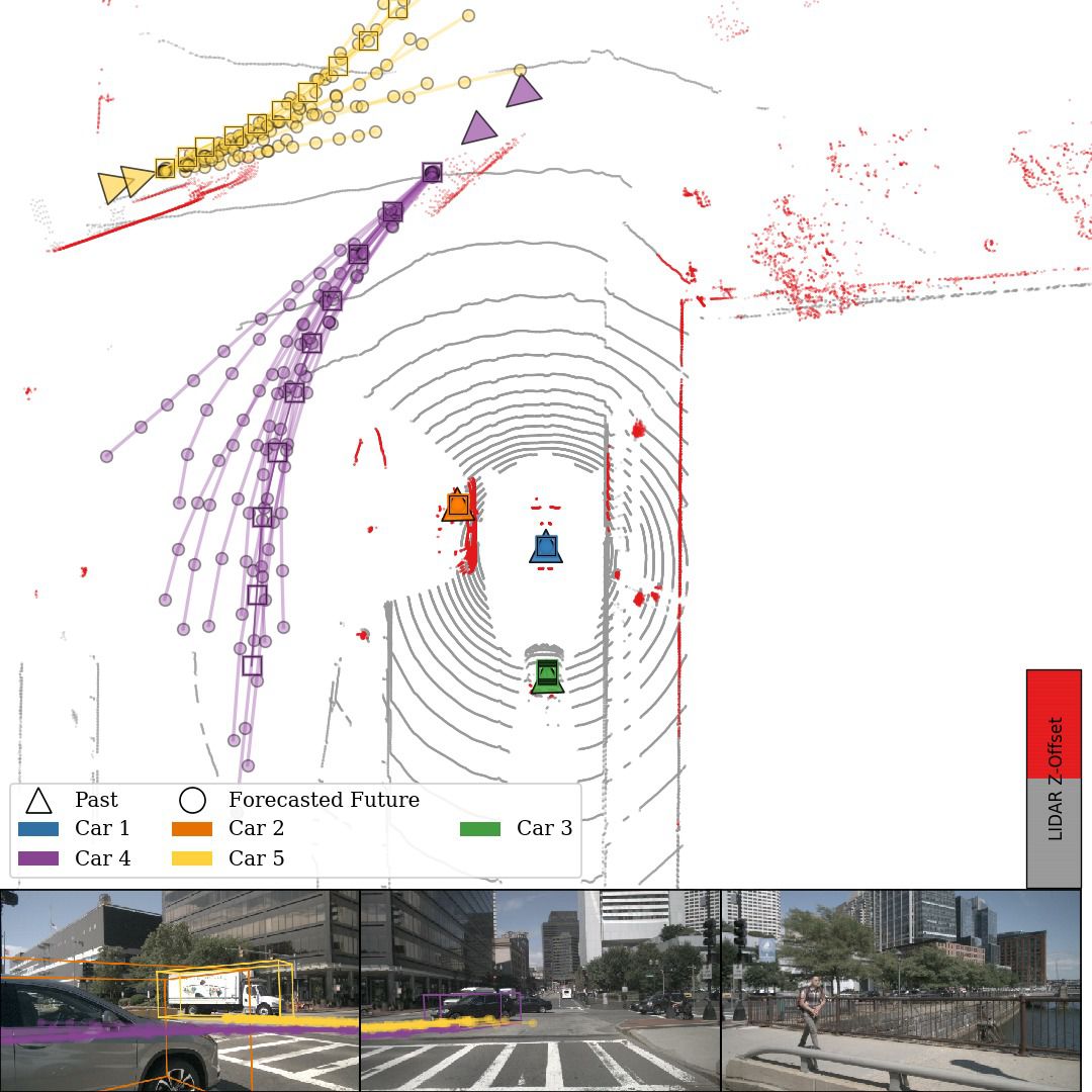
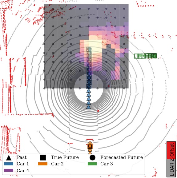
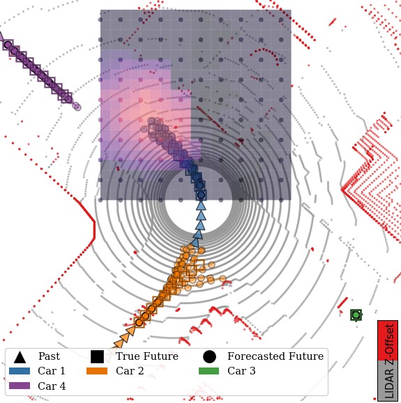
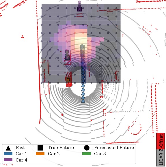
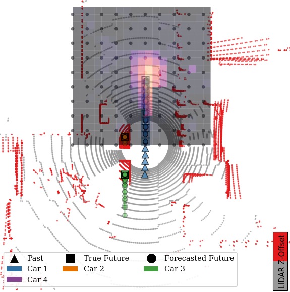
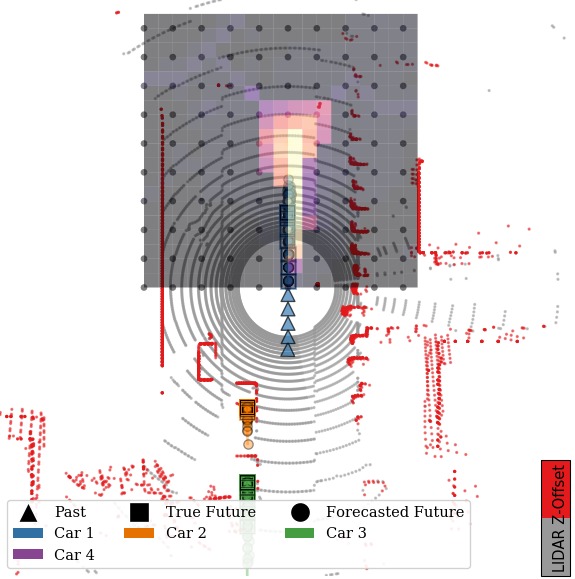
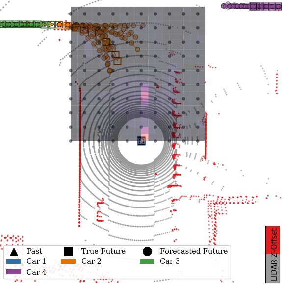
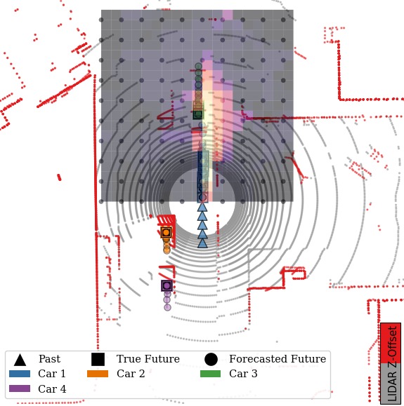
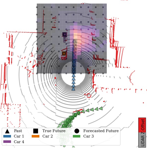
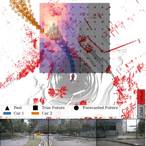
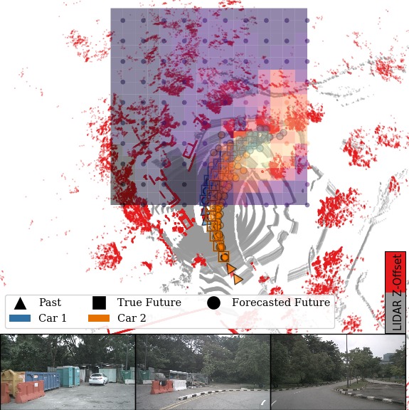
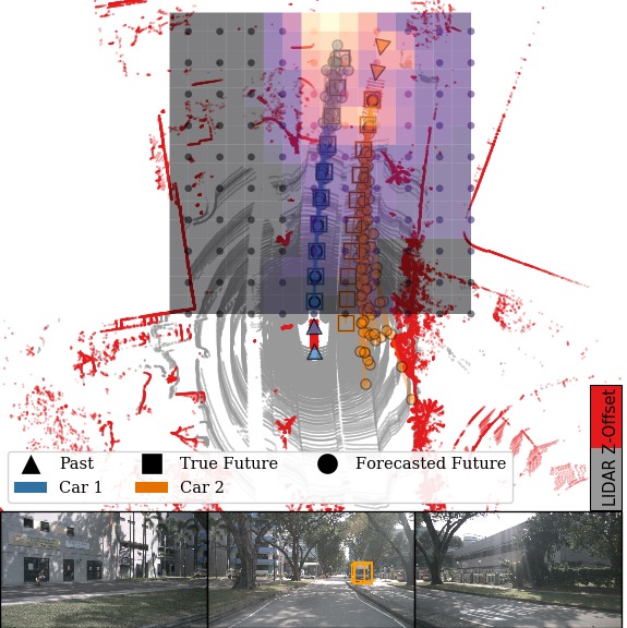
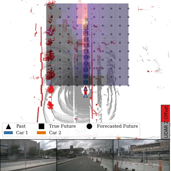
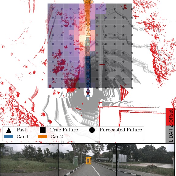
Autonomous driving requires reasoning about the future behaviors of agents in a variety of situations: at stop signs, roundabouts, crosswalks, when parking, when merging etc. In multi-agent settings, each agent’s behavior affects the behavior of others. Motivated by people’s ability to reason in these settings, we present a method to forecast multi-agent interactions from perceptual data, such as images and LIDAR. Beyond forecasting the behavior of all agents, we want our model to conditionally forecast how other agents are likely to respond to different decisions each agent could make. We want to forecast what other agents would likely do in response to a robot’s intention to achieve a goal. This reasoning is essential for agents to make good decisions in multi-agent environments: they must reason how their future decisions could affect the multi-agent system around them. Examples of forecasting and conditioning forecasts on robot goals are shown in Fig. 1 and Fig. 2. Videos of the outputs of our approach are available at https://sites.google.com/view/precog.

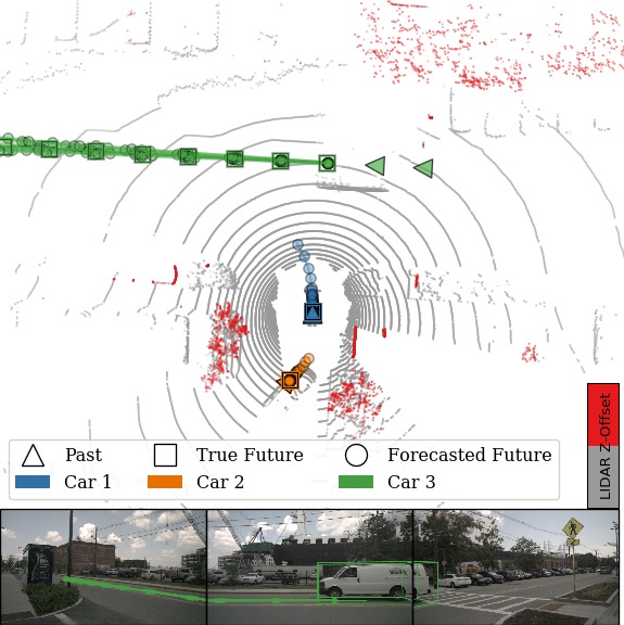
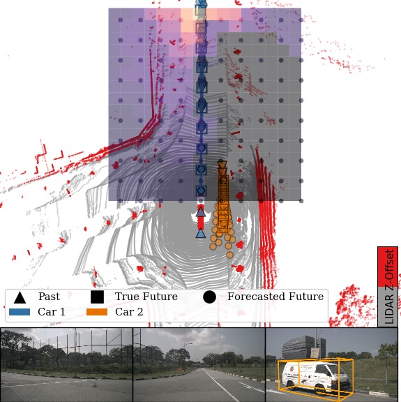
\begin{overpic}[width=204.88702pt,trim=2.84526pt 0.0pt 0.0pt 34.1433pt,clip]{fig/nuscenes/nuscenes_teaser_v4.jpg} \put(1.0,15.75){{\hbox{\pagecolor{white}{\color[rgb]{0,0,0}{ Left\vphantom{g}}}}}} \put(33.0,15.75){{\hbox{\pagecolor{white}{\color[rgb]{0,0,0}{ Front\vphantom{g}}}}}} \put(67.0,15.75){{\hbox{\pagecolor{white}{\color[rgb]{0,0,0}{ Right}}}}} \end{overpic}
Figure 1: Forecasting on nuScenes [4]. The input to our model is a high-dimensional LIDAR observation, which informs a distribution over all agents’ future trajectories.
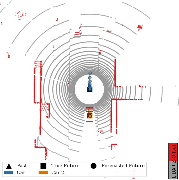
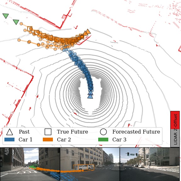
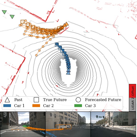
\begin{overpic}[width=153.93654pt]{fig/carla/carla_plan_teaser4.jpg} \put(2.0,96.5){{\hbox{\pagecolor{white}{\color[rgb]{0,0,0}{ \bf Forecasting \vphantom{g}}}}}} \put(2.0,66.5){{\hbox{\pagecolor{white}{\color[rgb]{0,0,0}{ \bf Conditional Forecast:\, Set Car 1 Goal=Ahead\vphantom{g}}}}}} \put(2.0,36.0){{\hbox{\pagecolor{white}{\color[rgb]{0,0,0}{ \bf Conditional Forecast:\, Set Car 1 Goal=Stop\vphantom{g}}}}}} \par\put(60.0,49.0){{\hbox{\pagecolor{white}{\color[rgb]{0.7109375,0.08984375,0}{ Goal=Ahead\vphantom{g}}}}}} \put(43.0,19.0){{\hbox{\pagecolor{white}{\color[rgb]{0.7109375,0.08984375,0}{ Goal=Stop \vphantom{g}}}}}} \par\put(34.0,81.0){{\hbox{\pagecolor{white}{\color[rgb]{0.21484375,0.4921875,0.72265625}{ Car 1\vphantom{g}}}}}} \put(34.0,49.0){{\hbox{\pagecolor{white}{\color[rgb]{0.21484375,0.4921875,0.72265625}{ Car 1\vphantom{g}}}}}} \put(34.0,19.0){{\hbox{\pagecolor{white}{\color[rgb]{0.21484375,0.4921875,0.72265625}{ Car 1\vphantom{g}}}}}} \par\put(34.0,97.0){{\hbox{\pagecolor{white}{\color[rgb]{1,0.49609375,0}{ Car 2\vphantom{g}}}}}} \par\put(5.0,81.5){{\hbox{\pagecolor{white}{\color[rgb]{0.30078125,0.6875,0.2890625}{ Car 3\vphantom{g}}}}}} \put(5.0,48.5){{\hbox{\pagecolor{white}{\color[rgb]{0.30078125,0.6875,0.2890625}{ Car 3\vphantom{g}}}}}} \put(5.0,19.0){{\hbox{\pagecolor{white}{\color[rgb]{0.30078125,0.6875,0.2890625}{ Car 3\vphantom{g}}}}}} \par\end{overpic}
Figure 2: Conditioning the model on different Car 1 goals produces different predictions: here it forecasts Car 3 to move if Car 1 yields space, or stay stopped if Car 1 stays stopped.

Throughout the paper, we use goal to mean a future states that an agent desires. Planning means the algorithmic process of producing a sequence of future decisions (in our model, choices of latent values) likely to satisfy a goal. Forecasting means the prediction of a sequence of likely future states; forecasts can either be single-agent or multi-agent. Finally, conditional forecasting means forecasting by conditioning on one or more agent goals. By planning an agent’s decisions to a goal and sampling from the other agents’s stochastic decisions, we perform multi-agent conditional forecasting. Although we plan future decisions in order to perform conditional forecasting, executing these plans on the robot is outside the scope of this work.

Towards conditional forecasting, we propose a factorized flow-based generative model that forecasts the joint state of all agents. Our model reasons probabilistically about plausible future interactions between agents given rich observations of their environment. It uses latent variables to capture the uncertainty in other agents’ decisions. Our key idea is the use of factorized latent variables to model decoupled agent decisions even though agent dynamics are coupled. Factorization across agents and time enable us to query the effects of changing an arbitrary agent’s decision at an arbitrary time step. Our contributions are:

  1. 1.

    State-of-the-art multi-agent vehicle forecasting: We develop a multi-agent forecasting model called Estimating Social-forecast Probabilities (ESP) that uses exact likelihood inference (unlike VAEs or GANs) to outperform three state-of-the-art methods on real and simulated vehicle datasets [4, 8].

  2. 2.

    Goal-conditioned multi-agent forecasting: We present the first generative multi-agent forecasting method able to condition on agent goals, called PREdiction Conditioned on Goals (PRECOG). After modelling agent interactions, conditioning on one agent’s goal alters the predictions of other agents.

  3. 3.

    Multi-agent imitative planning objective: We derive a data-driven objective for motion planning in multi-agent environments. It balances the likelihood of reaching a goal with the probability that expert demonstrators would execute the same plan. We use this objective for offline planning to known goals, which improves forecasting performance.

2 Related Work

Multi-agent modeling and forecasting is a challenging problem for control applications in which agents react to each other concurrently. Safe control requires faithful models of reality to anticipate dangerous situations before they occur. Modeling dependencies between agents is especially critical in tightly-coupled scenarios such as intersections.

Game-theoretic planning: Traditionally, multi-agent planning and game theory approaches explicitly model multiple agents’ policies or internal states, usually by generalizing Markov decision processes (MDPs) to multiple decisions makers [5, 35]. These frameworks facilitate reasoning about collaboration strategies, but suffer from “state space explosion” intractability except when interactions are known to be sparse [24] or hierarchically decomposable [11].

Multi-agent forecasting: Data-driven approaches have been applied to forecast complex interactions between multiple pedestrians [1, 3, 10, 14, 21], vehicles [6, 19, 26], and athletes [9, 18, 20, 34, 36, 37]. These methods attempt to generalize from previously observed interactions to predict multi-agent behavior in new situations. Forecasting is related to Imitation Learning [25], which learns a model to mimic demonstrated behavior. In contrast to some Imitation Learning methods, e.g. behavior cloning [29], behavior forecasting models are not executed in the environment of the observed agent – they are instead predictive models of the agent. In this sense, forecasting can be considered non-interactive Imitation Learning without execution.

Forecasting for control and planning: Generative models for multi-agent forecasting and control have been proposed. In terms of multi-agent forecasting, our work is related to [33] which uses a conditional VAE [17] encoding of the joint states of multiple agents together with recurrent cells to predict future human actions. However, our work differs in three crucial ways. First, we model continual co-influence between agents, versus “robot-only influence” where a robot’s responses to the human are not modeled. Second, our method uses contextual visual information useful for generalization to many new scenes. Third, we model interactions between more than two vehicles jointly. While [15] assumes conditional independencies for computational reasons, we do not, as they impose minimal overhead.

We consider scenarios in which the model may control one of the agents (a “robot”). In terms of planned control, our method generalizes imitative models [31]. In [31], single-agent forecasting models are used for deterministic single-agent planning. Our work instead considers multi-agent forecasting, and therefore must plan over a distribution of possible paths: from our robot’s perspective, the future actions of other human drivers are uncertain. By modeling co-influence, our robot’s trajectory are conditional on the (uncertain) future human trajectories, and therefore future robots states are necessarily uncertain. Thus, our work proposes a nontrivial extension for imitative models: we consider future path planning uncertainty induced by the uncertain actions of other agents in a multi-agent setting. While [31] could implicitly model other agents through its visual conditioning, we show explicit modeling of other agents yields better forecasting results, in addition to giving us the tools to predict responses to agent’s plans.

3 Deep Multi-Agent Forecasting

In this section, we will describe our likelihood-based model for multi-agent forecasting, and then describe how we use it to perform planning and multi-agent conditional forecasting. First, we define our notation and terminology. We treat our multi-agent system as a continuous-space, discrete-time, partially-observed Markov process, composed of A𝐴A agents (vehicles) that interact over T𝑇T time steps. We model all agent positions at time t𝑡t as 𝐒tA×Dsubscript𝐒𝑡superscript𝐴𝐷\mathbf{S}_{t}\in\mathbb{R}^{A\times D}, where D=2𝐷2D\!=\!2. 𝐒tasuperscriptsubscript𝐒𝑡𝑎\mathbf{S}_{t}^{a} represents agent a𝑎a’s (x,y)𝑥𝑦(x,y) coordinates on the ground plane. We assume there is one “robot agent” (e.g. the AV) and A1𝐴1A\!-\!1 “human agents” (e.g. human drivers that our model cannot control). We define 𝐒tr𝐒t1Dapproaches-limitsuperscriptsubscript𝐒𝑡𝑟superscriptsubscript𝐒𝑡1superscript𝐷\mathbf{S}_{t}^{r}\doteq\mathbf{S}_{t}^{1}\in\mathbb{R}^{D} to index the robot state, and 𝐒th𝐒t2:A(A1)×Dapproaches-limitsuperscriptsubscript𝐒𝑡superscriptsubscript𝐒𝑡:2𝐴superscript𝐴1𝐷\mathbf{S}_{t}^{h}\doteq\mathbf{S}_{t}^{2:A}\in\mathbb{R}^{(A-1)\times D} to index the human states. Bold font distinguishes variables from functions. Capital English letters denote random variables. We define t=0𝑡0t\!=\!0 to be the current time. Subscript absence denotes all future time steps, and superscript absence denotes all agents, e.g. 𝐒𝐒1:T1:AT×A×Dapproaches-limit𝐒superscriptsubscript𝐒:1𝑇:1𝐴superscript𝑇𝐴𝐷\mathbf{S}\doteq\mathbf{S}_{1:T}^{1:A}\in\mathbb{R}^{T\times A\times D}.

Each agent has access to environment perception ϕ{𝐬τ:0,𝝌}approaches-limititalic-ϕsubscript𝐬:𝜏0𝝌\phi\doteq\{\mathbf{s}_{-\tau:0},\bm{\chi}\}, where τ𝜏\tau is the number of past multi-agent positions we condition on and 𝝌𝝌\bm{\chi} is a high-dimensional observation of the scene. 𝝌𝝌\bm{\chi} might represent LIDAR or camera images, and is the robot’s observation of the world. In our setting, LIDAR is provided as 𝝌=200×200×2𝝌superscript2002002\bm{\chi}=\mathbb{R}^{200\times 200\times 2}, with 𝝌ijsubscript𝝌𝑖𝑗\bm{\chi}_{ij} representing a 2-bin histogram of points above and at ground level in 0.5m20.5superscriptm20.5\mathrm{m}^{2} cells. Although our perception is robot-centric, each agent is modeled to have access to 𝝌𝝌\bm{\chi}.

3.1 Estimating Social-forecast Probability (ESP)

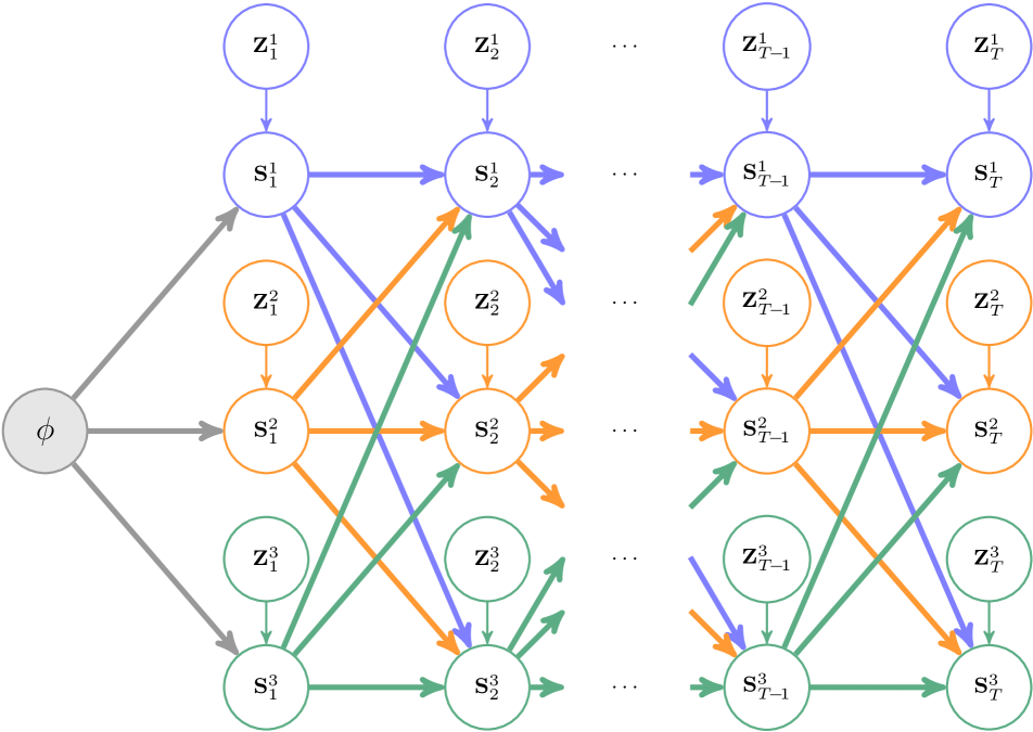
We propose a data-driven likelihood-based generative model of multi-agent interaction to probabilistically predict T𝑇T-step dynamics of a multi-agent system: 𝐒q(𝐒|ϕ;𝒟)similar-to𝐒𝑞conditional𝐒italic-ϕ𝒟\mathbf{S}\!\sim\!q(\mathbf{S}|\phi;\!\mathcal{D}), where 𝒟𝒟\mathcal{D} is training data of observed multi-agent state trajectories. Our model learns to map latent variables 𝐙𝐙\mathbf{Z} via an invertible function f𝑓f to multi-agent trajectories 𝐒𝐒\mathbf{S} conditioned on ϕitalic-ϕ\phi. f𝑓f’s invertibility induces q(𝐒|ϕ)𝑞conditional𝐒italic-ϕq(\mathbf{S}|\phi), a pushforward distribution [23], also known as an invertible generative model [7, 12, 13, 16, 30]. Invertible generative models can efficiently and exactly compute probabilities of samples. Here, it means we can compute the probability of joint multi-agent trajectories, critical to our goal of planning with the model. We name the model “Estimating Social-forecast Probabilities” (ESP). 𝐒𝐒\mathbf{S} is sampled from q𝑞q as follows:

𝐙𝒩(𝟎,𝐈);𝐒=f(𝐙;ϕ);𝐒,𝐙T×A×D.formulae-sequencesimilar-to𝐙𝒩0𝐈formulae-sequence𝐒𝑓𝐙italic-ϕ𝐒𝐙superscript𝑇𝐴𝐷\textstyle\mathbf{Z}\sim\mathcal{N}(\mathbf{0},\mathbf{I});\quad\mathbf{S}=f(\mathbf{Z};\phi);\quad\mathbf{S},\mathbf{Z}\in\mathbb{R}^{T\times A\times D}. (1)

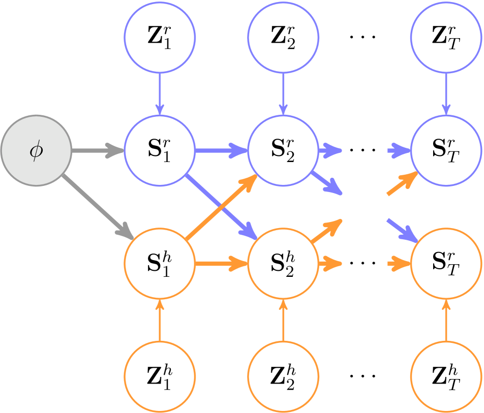
Our latent variables 𝐙𝐙1:T1:Aapproaches-limit𝐙superscriptsubscript𝐙:1𝑇:1𝐴\mathbf{Z}\doteq\mathbf{Z}_{1:T}^{1:A} factorize across agents and time, which allows us to decide agent a𝑎a’s reaction at time t𝑡t by setting 𝐙ta𝐳tasuperscriptsubscript𝐙𝑡𝑎superscriptsubscript𝐳𝑡𝑎\mathbf{Z}_{t}^{a}\leftarrow\mathbf{z}_{t}^{a}, discussed later. Our model is related to the R2P2 single-agent generative model [30], which constructs a deep likelihood-based generative model for single-agent vehicle forecasting. For multi-step prediction, we generalize R2P2’s autoregressive one-step single-agent prediction for the multi-agent setting, and assume a one-step time delay for agents to react to each other:

𝐒ta=μθa(𝐒1:t1,ϕ)+σθa(𝐒1:t1,ϕ)𝐙taD,superscriptsubscript𝐒𝑡𝑎superscriptsubscript𝜇𝜃𝑎subscript𝐒:1𝑡1italic-ϕsuperscriptsubscript𝜎𝜃𝑎subscript𝐒:1𝑡1italic-ϕsuperscriptsubscript𝐙𝑡𝑎superscript𝐷\textstyle\mathbf{S}_{t}^{a}\;=\;\mu_{\theta}^{a}(\mathbf{S}_{1:t-1},\phi)+\sigma_{\theta}^{a}(\mathbf{S}_{1:t-1},\phi)\cdot\mathbf{Z}_{t}^{a}\;\in\mathbb{R}^{D}, (2)

where μθa()superscriptsubscript𝜇𝜃𝑎\mu_{\theta}^{a}(\cdot) and σθa()superscriptsubscript𝜎𝜃𝑎\sigma_{\theta}^{a}(\cdot) are neural network functions (with trainable weights θ𝜃\theta) outputting a one-step mean prediction 𝝁taDsuperscriptsubscript𝝁𝑡𝑎superscript𝐷\bm{\mu}_{t}^{a}\in\mathbb{R}^{D} and standard-deviation matrix 𝝈taD×Dsuperscriptsubscript𝝈𝑡𝑎superscript𝐷𝐷\bm{\sigma}_{t}^{a}\in\mathbb{R}^{D\times D} of agent a𝑎a, defining the system’s transition function q𝑞q as

q(𝐒t|𝐒1:t1,ϕ)=a=1A𝒩(𝐒ta;𝝁ta,𝚺ta),𝑞conditionalsubscript𝐒𝑡subscript𝐒:1𝑡1italic-ϕsuperscriptsubscriptproduct𝑎1𝐴𝒩superscriptsubscript𝐒𝑡𝑎superscriptsubscript𝝁𝑡𝑎superscriptsubscript𝚺𝑡𝑎\textstyle q(\mathbf{S}_{t}|\mathbf{S}_{1:t-1},\phi)=\prod_{a=1}^{A}\mathcal{N}(\mathbf{S}_{t}^{a};\bm{\mu}_{t}^{a},\bm{\Sigma}_{t}^{a}), (3)

where 𝚺ta=𝝈ta𝝈tasuperscriptsubscript𝚺𝑡𝑎superscriptsubscript𝝈𝑡𝑎superscriptsubscript𝝈𝑡limit-from𝑎top\bm{\Sigma}_{t}^{a}=\bm{\sigma}_{t}^{a}\bm{\sigma}_{t}^{a\top}. Note that (2) predicts the athsuperscript𝑎tha^{\text{th}} agent’s state 𝐒tasuperscriptsubscript𝐒𝑡𝑎\mathbf{S}_{t}^{a} given the previous multi-agent states 𝐒1:t1subscript𝐒:1𝑡1\mathbf{S}_{1:t-1}. We can see that given 𝐒1:t1subscript𝐒:1𝑡1\mathbf{S}_{1:t-1}, the one-step prediction in (2) is unimodal Gaussian. However, multi-step predictions are generally multimodal given the recursive nonlinear conditioning of neural network outputs 𝝁tasuperscriptsubscript𝝁𝑡𝑎\bm{\mu}_{t}^{a} and 𝝈tasuperscriptsubscript𝝈𝑡𝑎\bm{\sigma}_{t}^{a} on previous predictions. The final joint of this model can be written as

q(𝐒|ϕ)𝑞conditional𝐒italic-ϕ\displaystyle\textstyle q(\mathbf{S}|\phi) =t=1Tq(𝐒t|𝐒1:t1,ϕ).absentsuperscriptsubscriptproduct𝑡1𝑇𝑞conditionalsubscript𝐒𝑡subscript𝐒:1𝑡1italic-ϕ\displaystyle=\textstyle\prod_{t=1}^{T}\!q(\mathbf{S}_{t}|\mathbf{S}_{1:t-1},\phi). (4)
Refer to caption
(a) ESP forecasting
Refer to caption
(b) PRECOG planning
Refer to caption
(c) ESP model implementation
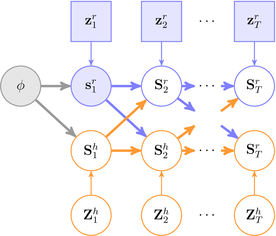
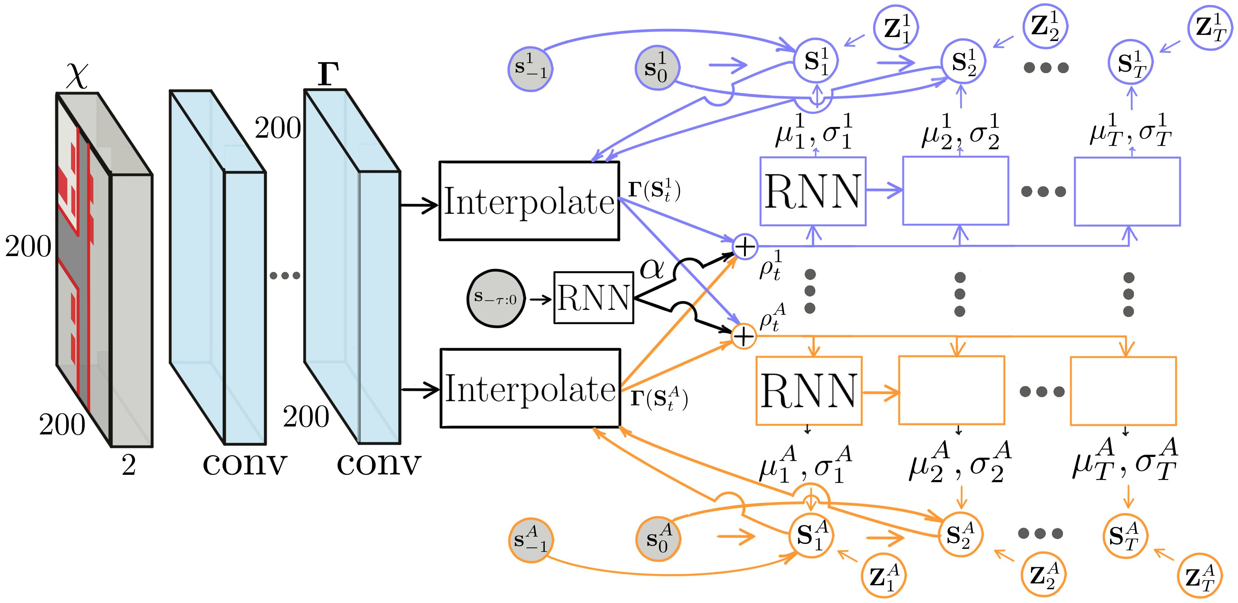
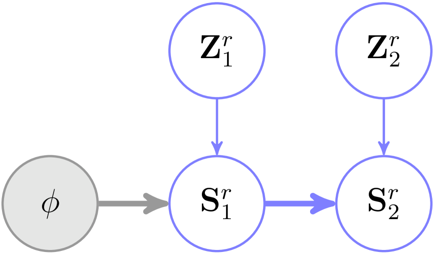
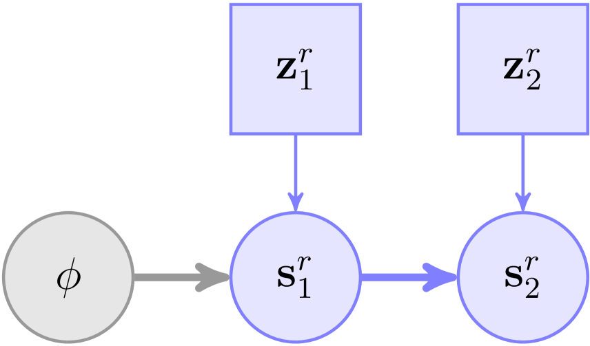
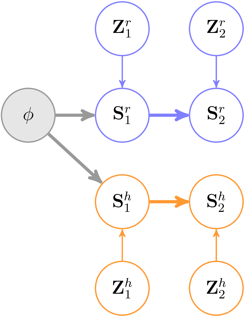
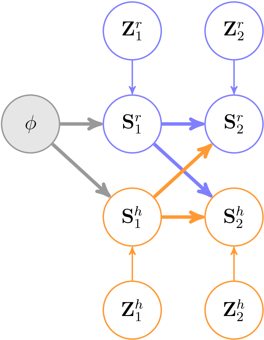
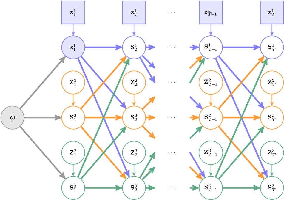
Figure 3: Our factorized latent variable model of forecasting and planning shown for 2 agents. In Fig. 3(a) our model uses latent variable 𝐙t+1asuperscriptsubscript𝐙𝑡1𝑎\mathbf{Z}_{t+1}^{a} to represent variation in agent a𝑎a’s plausible scene-conditioned reactions to all agents 𝐒tsubscript𝐒𝑡\mathbf{S}_{t}, causing uncertainty in every agents’ future states 𝐒𝐒\mathbf{S}. Variation exists because of unknown driver goals and different driving styles observed in the training data. Beyond forecasting, our model admits planning robot decisions by deciding 𝐙r=𝐳rsuperscript𝐙𝑟superscript𝐳𝑟\mathbf{Z}^{r}\!=\!\mathbf{z}^{r} (Fig. 3(b)). Shaded nodes represent observed or determined variables, and square nodes represent robot decisions [2]. Thick arrows represent grouped dependencies of non-Makovian 𝐒tsubscript𝐒𝑡\mathbf{S}_{t} “carried forward” (a regular edge exists between any pair of nodes linked by a chain of thick edges). Note 𝐙𝐙\mathbf{Z} factorizes across agents, isolating the robot’s reaction variable 𝐳rsuperscript𝐳𝑟\mathbf{z}^{r}. Human reactions remain uncertain (𝐙hsuperscript𝐙\mathbf{Z}^{h} is unobserved) and uncontrollable (the robot cannot decide 𝐙hsuperscript𝐙\mathbf{Z}^{h}), and yet the robot’s decisions 𝐳rsuperscript𝐳𝑟\mathbf{z}^{r} will still influence human drivers 𝐒2:Thsubscriptsuperscript𝐒:2𝑇\mathbf{S}^{h}_{2:T} (and vice-versa). Fig. 3(c) shows our implementation. See Appendix C for details.

3.2 Model Implementation

To implement our model q(𝐒|ϕ)𝑞conditional𝐒italic-ϕq(\mathbf{S}|\phi), we design neural networks that output 𝝁tasuperscriptsubscript𝝁𝑡𝑎\bm{\mu}_{t}^{a} and 𝝈tasuperscriptsubscript𝝈𝑡𝑎\bm{\sigma}_{t}^{a}. Similar to [30], we expand μθa()superscriptsubscript𝜇𝜃𝑎\mu_{\theta}^{a}(\cdot) to represent a “Verlet” step, which predicts a constant-velocity mean when 𝐦ta=mθa(𝐒1:t1,ϕ)=0superscriptsubscript𝐦𝑡𝑎subscriptsuperscript𝑚𝑎𝜃subscript𝐒:1𝑡1italic-ϕ0\mathbf{m}_{t}^{a}=m^{a}_{\theta}(\mathbf{S}_{1:t\!-\!1},\!\phi)=0:

𝐒ta=2𝐒t1a𝐒t2a+mθa(𝐒1:t1,ϕ)𝝁ta+σθa(𝐒1:t1,ϕ)𝝈ta𝐙ta.subscriptsuperscript𝐒𝑎𝑡subscript2subscriptsuperscript𝐒𝑎𝑡1subscriptsuperscript𝐒𝑎𝑡2subscriptsuperscript𝑚𝑎𝜃subscript𝐒:1𝑡1italic-ϕsuperscriptsubscript𝝁𝑡𝑎subscriptsubscriptsuperscript𝜎𝑎𝜃subscript𝐒:1𝑡1italic-ϕsuperscriptsubscript𝝈𝑡𝑎subscriptsuperscript𝐙𝑎𝑡\textstyle\mathbf{S}^{a}_{t}=\underbrace{2\mathbf{S}^{a}_{t\!-\!1}\!\!-\!\mathbf{S}^{a}_{t\!-\!2}\!\!+\!m^{a}_{\theta}(\mathbf{S}_{1:t\!-\!1},\!\phi)}_{\bm{\mu}_{t}^{a}}+\underbrace{\sigma^{a}_{\theta}(\mathbf{S}_{1:t\!-\!1},\!\phi)}_{\bm{\sigma}_{t}^{a}}\cdot\mathbf{Z}^{a}_{t}. (5)

A high-level diagram of our implementation shown in Fig. 3(c). Recall ϕ={𝐬τ:0,𝝌}italic-ϕsubscript𝐬:𝜏0𝝌\phi\!=\!\{\mathbf{s}_{-\tau:0},\bm{\chi}\}: the context contains the past positions of all agents, 𝐬τ:0subscript𝐬:𝜏0\mathbf{s}_{-\tau:0}, and a feature map 𝝌𝝌\bm{\chi}, implemented as LIDAR observed by the robot. We encode 𝐬τ:0subscript𝐬:𝜏0\mathbf{s}_{-\tau:0} with a GRU. A CNN processes 𝝌𝝌\bm{\chi} to 𝚪𝚪\bm{\Gamma} at the same spatial resolution as 𝝌𝝌\bm{\chi}. Features for each agent’s predicted position 𝐒tasuperscriptsubscript𝐒𝑡𝑎\mathbf{S}_{t}^{a} are computed by interpolating into 𝚪𝚪\bm{\Gamma} as 𝚪(𝐒ta)𝚪superscriptsubscript𝐒𝑡𝑎\bm{\Gamma}(\mathbf{S}_{t}^{a}). Positional “social features” for agent a𝑎a are computed: 𝐒ta𝐒tbbA{a}superscriptsubscript𝐒𝑡𝑎superscriptsubscript𝐒𝑡𝑏for-all𝑏𝐴𝑎\mathbf{S}_{t}^{a}\!-\!\mathbf{S}_{t}^{b}~{}\forall~{}b\!\in\!A\!\setminus\!\{a\}, as well as visual “social features” γta=𝚪(𝐬t1)𝚪(𝐬tA)superscriptsubscript𝛾𝑡𝑎direct-sum𝚪superscriptsubscript𝐬𝑡1𝚪superscriptsubscript𝐬𝑡𝐴\gamma_{t}^{a}=\bm{\Gamma}(\mathbf{s}_{t}^{1})\oplus\dots\oplus\bm{\Gamma}(\mathbf{s}_{t}^{A}). The social features, past encoding, and CNN features are fed to a per-agent GRU, which produces 𝐦tasubscriptsuperscript𝐦𝑎𝑡\mathbf{m}^{a}_{t} and 𝝈tasuperscriptsubscript𝝈𝑡𝑎\bm{\sigma}_{t}^{a} in (5). We train with observations of expert multi-agent interaction 𝐒p(𝐒|ϕ)similar-tosuperscript𝐒𝑝conditionalsuperscript𝐒italic-ϕ\mathbf{S}^{*}\sim p(\mathbf{S}^{*}|\phi) by maximizing likelihood with respect to our model parameters θ𝜃\theta. We use shared parameters to produce 𝚪𝚪\bm{\Gamma} and the past encoding. See Appendix C for an architecture table and other details.

Flexible-count implementation: While the implementation described so far is limited to predict for a fixed-count of agents in a scene, we also implemented a flexible-count version. There are two flavors of a model that is flexible in practice. (1) A fully-flexible model applicable to any scene with agent count Atestsubscript𝐴testA_{\text{test}}\in\mathbb{N}. (2) A partially-flexible model applicable to any scene with agent count Atest{1..Atrain}A_{\text{test}}\in\{1..A_{\text{train}}\}, controlled by a hyperparameter upper-bound Atrainsubscript𝐴trainA_{\text{train}} set at training time. To implement (1), the count of model parameters must be independent of Atestsubscript𝐴testA_{\text{test}} in order for the same architecture to apply to scenes with different counts of agents. To implement (2), “missing agents” must not affect the joint distribution over the existing agents, equivalent to ensuring 𝐒existing/𝐙missing=0superscript𝐒existingsuperscript𝐙missing0\nicefrac{{\partial\mathbf{S}^{\text{existing}}}}{{\partial\mathbf{Z}^{\text{missing}}}}\!=\!0 in our framework. We implemented (2) by using a mask M{0,1}Atrain𝑀superscript01subscript𝐴trainM\!\in\!\{0,1\}^{A_{\text{train}}} to mask features of missing agents. In this model, we shared parameters across agents, and trained it on data with varying counts of agents.

3.3 Conditional Forecasting

A distinguishing feature of our generative model for multi-step, multi-agent prediction is its latent variables 𝐙𝐙1:T1:Aapproaches-limit𝐙superscriptsubscript𝐙:1𝑇:1𝐴\mathbf{Z}\doteq\mathbf{Z}_{1:T}^{1:A} that factorizes over agents and time. Factorization makes it possible to use the model for highly flexible conditional forecasts. Conditional forecasts predict how other agents would likely respond to different robot decisions at different moments in time. Since robots are not merely passive observers, but one of potentially many agents, the ability to anticipate how they affect others is critical to their ability to plan useful, safe, and effective actions, critical to their utility within a planning and control framework [22].

Human drivers can appear to take highly stochastic actions in part because we cannot observe their goals. In our model, the source of this uncertainty comes from the latent variables 𝐙𝒩(𝟎,𝐈)similar-to𝐙𝒩0𝐈\mathbf{Z}\!\sim\!\mathcal{N}(\mathbf{0},\mathbf{I}). In practical scenarios, the robot knows its own goals, can choose its own actions, and can plan a course of action to achieve a desired goal. Recall from (2) that one-step agent predictions are conditionally independent from each other give the previous multi-agent states. Therefore, certainty in the latent state 𝐙tasuperscriptsubscript𝐙𝑡𝑎\mathbf{Z}_{t}^{a} corresponds to certainty of the athsuperscript𝑎tha^{\text{th}} agent’s reaction at time t𝑡t to the multi-agent system history 𝐒1:t1subscript𝐒:1𝑡1\mathbf{S}_{1:t-1}. Different values of 𝐙tasuperscriptsubscript𝐙𝑡𝑎\mathbf{Z}_{t}^{a} correspond to different ways of reacting to the same information. Deciding values of 𝐙tasuperscriptsubscript𝐙𝑡𝑎\mathbf{Z}_{t}^{a} corresponds to controlling the agent a𝑎a. We can therefore implement control of the robot via assigning values to its latent variables 𝐙r𝐳rsuperscript𝐙𝑟superscript𝐳𝑟\mathbf{Z}^{r}\leftarrow\mathbf{z}^{r}. In contrast, human reactions 𝐙thsuperscriptsubscript𝐙𝑡\mathbf{Z}_{t}^{h} cannot be decided by the robot, but remain uncertain from the robot’s perspective. Thus, humans can only be influenced by their conditioning on the robot’s previous states in 𝐒1:t1subscript𝐒:1𝑡1\mathbf{S}_{1:t-1}, as seen Fig. 3(b). Therefore, to generate conditional-forecasts, we decide 𝐳rsuperscript𝐳𝑟\mathbf{z}^{r}, sample 𝐙hsuperscript𝐙\mathbf{Z}^{h}, concatenate 𝐙=𝐳r𝐙h𝐙direct-sumsuperscript𝐳𝑟superscript𝐙\mathbf{Z}\!=\!\mathbf{z}^{r}\oplus\mathbf{Z}^{h}, and warp 𝐒=f(𝐙,ϕ)𝐒𝑓𝐙italic-ϕ\mathbf{S}\!=\!f(\mathbf{Z},\phi). This factorization of latent variables easily facilitates conditional forecasting. To forecast 𝐒𝐒\mathbf{S}, we can fix 𝐳rsuperscript𝐳𝑟\mathbf{z}^{r} while sampling the human agents’ reactions from their distribution p(𝐙h)=𝒩(𝟎,𝐈)𝑝superscript𝐙𝒩0𝐈p(\mathbf{Z}^{h})\!=\!\mathcal{N}(\mathbf{0},\mathbf{I}), which are warped via (1).

3.4 PREdiction Conditioned On Goals (PRECOG)

We discussed how forecasting can condition on a value of 𝐳rsuperscript𝐳𝑟\mathbf{z}^{r}, but not yet how to find desirable values of 𝐳rsuperscript𝐳𝑟\mathbf{z}^{r}, e.g. values that would safely direct the robot towards its goal location. We perform multi-agent planning by optimizing an objective \mathcal{L} w.r.t. the control variables 𝐳rsuperscript𝐳𝑟\mathbf{z}^{r}, which allows us to produce the “best” forecasts under \mathcal{L}.

While many objectives are valid, we use imitative models (IM), which estimate the likeliest state trajectory an expert “would have taken” to satisfy a goal, based on prior expert demonstrations [31]. IM modeled single-agent environments where robot trajectories are planned without consideration of other agents. Multi-agent planning is different, because future robot states are uncertain (states 𝐒t>1rsubscriptsuperscript𝐒𝑟𝑡1\mathbf{S}^{r}_{t>1} in Fig. 3(b)), even when conditioned on control variables 𝐳rsuperscript𝐳𝑟\mathbf{z}^{r}, because of the uncertainty in surrounding human drivers 𝐙hsuperscript𝐙\mathbf{Z}^{h}.

We generalize IM to multi-agent environments, and plan w.r.t. the uncertainty of human drivers close by. First, we chose a “goal likelihood” function that represents the likelihood that a robot reaches its goal 𝒢𝒢\mathcal{G} given state trajectory 𝐒𝐒\mathbf{S}. For instance, the likelihood could be a waypoint 𝐰D𝐰superscript𝐷\mathbf{w}\!\in\!\mathbb{R}^{D} the robot should approach: p(𝒢|𝐒,ϕ)=𝒩(𝐰;𝐒Tr,ϵ𝐈)𝑝conditional𝒢𝐒italic-ϕ𝒩𝐰subscriptsuperscript𝐒𝑟𝑇italic-ϵ𝐈p(\mathcal{G}|\mathbf{S},\phi)\!=\!\mathcal{N}(\mathbf{w};\mathbf{S}^{r}_{T},\epsilon\mathbf{I}). Second, we combine the goal likelihood with a “prior probability” model of safe multi-agent state trajectories q(𝐒|ϕ)𝑞conditional𝐒italic-ϕq(\mathbf{S}|\phi), learned from expert demonstrations. Note that unlike many other generative multi-agent models, we can compute the probability of generating 𝐒𝐒\mathbf{S} from q(𝐒|ϕ)𝑞conditional𝐒italic-ϕq(\mathbf{S}|\phi) exactly, which is critical to our planning approach. This results in a “posterior” p(𝐒|𝒢,ϕ)𝑝conditional𝐒𝒢italic-ϕp(\mathbf{S}|\mathcal{G},\phi). Finally, we plan a goal-seeking path in the learned distribution of demonstrated multi-agent behavior under the log-posterior probability derived as:

log\displaystyle\textstyle\log 𝔼𝐙h[p(𝐒|𝒢,ϕ)]𝔼𝐙h[logp(𝐒|𝒢,ϕ)]subscript𝔼superscript𝐙delimited-[]𝑝conditional𝐒𝒢italic-ϕsubscript𝔼superscript𝐙delimited-[]𝑝conditional𝐒𝒢italic-ϕ\displaystyle\textstyle\,\mathbb{E}_{\mathbf{Z}^{h}}[p(\mathbf{S}|\mathcal{G},\phi)]\textstyle\;\geq\;\textstyle\mathbb{E}_{\mathbf{Z}^{h}}[\log p(\mathbf{S}|\mathcal{G},\phi)] (6)
=𝔼𝐙h[log(q(𝐒|ϕ)p(𝒢|𝐒,ϕ))]logp(𝒢|ϕ)absentsubscript𝔼superscript𝐙delimited-[]𝑞conditional𝐒italic-ϕ𝑝conditional𝒢𝐒italic-ϕ𝑝conditional𝒢italic-ϕ\displaystyle=\mathbb{E}_{\mathbf{Z}^{h}}[\log\big{(}q(\mathbf{S}|\phi)p(\mathcal{G}|\mathbf{S},\phi)\big{)}]\!-\!\log p(\mathcal{G}|\phi) (7)
(𝐳r,𝒢)superscript𝐳𝑟𝒢\displaystyle\mathcal{L}(\mathbf{z}^{r},\mathcal{G}) 𝔼𝐙h[logq(𝐒|ϕ)+logp(𝒢|𝐒,ϕ)]approaches-limitabsentsubscript𝔼superscript𝐙delimited-[]𝑞conditional𝐒italic-ϕ𝑝conditional𝒢𝐒italic-ϕ\displaystyle\doteq\mathbb{E}_{\mathbf{Z}^{h}}[\log q(\mathbf{S}|\phi)+\log p(\mathcal{G}|\mathbf{S},\phi)] (8)
=𝔼𝐙h[logq(f(𝐙)|ϕ)multi-agent prior+logp(𝒢|f(𝐙),ϕ)goal likelihood],absentsubscript𝔼superscript𝐙delimited-[]subscript𝑞conditional𝑓𝐙italic-ϕmulti-agent priorsubscript𝑝conditional𝒢𝑓𝐙italic-ϕgoal likelihood\displaystyle=\mathbb{E}_{\mathbf{Z}^{h}}[\log\!\!\underbrace{q(f(\mathbf{Z})|\phi)}_{\text{multi-agent prior}}\!\!+\log\underbrace{p(\mathcal{G}|f(\mathbf{Z}),\phi)}_{\text{goal likelihood}}], (9)

where (6) follows by Jensen’s inequality, which we use to avoid the numerical issue of a single sampled 𝐙hsuperscript𝐙\mathbf{Z}^{h} dominating the batch. (7) follows from Bayes’ rule and uses our learned model q𝑞q as the prior. In (8), we drop p(𝒢|ϕ)𝑝conditional𝒢italic-ϕp(\mathcal{G}|\phi) because it is constant w.r.t. 𝐳rsuperscript𝐳𝑟\mathbf{z}^{r}. Recall 𝐙=𝐳r𝐙h𝐙direct-sumsuperscript𝐳𝑟superscript𝐙\mathbf{Z}=\mathbf{z}^{r}\oplus\mathbf{Z}^{h} is the concatenation of robot and human control variables. The robot can plan using our ESP model by optimizing (9):

𝐳r=argmax𝐳r(𝐳r,𝒢).superscript𝐳𝑟subscriptargmaxsuperscript𝐳𝑟superscript𝐳𝑟𝒢\textstyle\mathbf{z}^{r*}=\operatorname*{argmax}_{\mathbf{z}^{r}}\mathcal{L}(\mathbf{z}^{r},\mathcal{G}). (10)

Other objectives might be used instead, e.g. maximizing the posterior probability of the robot trajectories only. This may place human agents in unusual, precarious driving situations, outside the prior distribution of “usual driving interaction”. (10) encourages the robot to avoid actions likely to put the joint system in an unexpected situation.

4 Experiments

We first compare our forecasting model against existing state-of-the-art multi-agent forecasting methods, including SocialGAN [14], DESIRE [19]. We also include a baseline model: R2P2-MA (adapted from R2P2 [30] to instead handle multiple agent inputs), which does not model how agents will react to each others’ future decisions. Second, we investigate the novel problem of conditional forecasting. To quantify forecasting performance, we study scenarios where we have pairs of the robot’s true goal and the sequence of joint states. Knowledge of goals should enable our model to better predict what the robot and each agent could do. Third, we ablate the high-dimensional contextual input 𝝌𝝌\bm{\chi} from our model to determine its relevance to forecasting. Appendix F and G provide: (1) more conditional forecasting results, (2) localization sensitivity analysis and mitigation (3) evaluations on more datasets, and (4) several pages of qualitative results.

nuScenes dataset: We used the recently-released full nuScenes dataset [4], a real-world dataset for multi-agent trajectory forecasting, in which 850 episodes of 20 seconds of driving were recorded and labelled at 2Hz with the positions of all agents, and synced with many sensors, including LIDAR. We processed each of the examples to train, val, and test splits. Each example has 2 seconds of past and 4 seconds of future positions at 5Hz and is accompanied by a LIDAR map composited from 1 second of previous scans. We also experimented concatenating a binary road mask to χ𝜒\chi, indicated as “Road” in our evaluation.

CARLA dataset: We generated a realistic dataset for multi-agent trajectory forecasting and planning with the CARLA simulator [8]. We ran the autopilot in Town01 for over 900 episodes of 100 seconds each in the presence of 100 other vehicles, and recorded the trajectory of every vehicle and the autopilot’s LIDAR observation. We randomized episodes to either train, validation, or test sets. We created sets of 607016070160701 train, 758675867586 validation, and 756775677567 test examples, each with 2 seconds of past and 2 seconds of future positions at 10Hz. See Appendix E for details and https://sites.google.com/view/precog for data.

4.1 Metrics

Log-likelihood: As our models can perform exact likelihood inference (unlike GANs or VAEs), we can precisely evaluate how likely held-out samples are under each model. Test log-likelihood is given by the forward cross-entropy H(p,q)=𝔼𝐒p(𝐒|ϕ)logq(𝐒|ϕ)𝐻𝑝𝑞subscript𝔼similar-tosuperscript𝐒𝑝conditionalsuperscript𝐒italic-ϕ𝑞conditionalsuperscript𝐒italic-ϕH(p,q)\!=\!-\mathbb{E}_{\mathbf{S}^{*}\sim p(\mathbf{S}^{*}|\phi)}\log q(\mathbf{S}^{*}|\phi), which is unbounded for general p𝑝p and q𝑞q. However, by perturbing samples from p(𝐒|ϕ)𝑝conditionalsuperscript𝐒italic-ϕp(\mathbf{S}^{*}|\phi) with noise drawn from a known distribution η𝜂\eta (e.g. a Gaussian) to produce a perturbed distribution psuperscript𝑝p^{\prime}, we can enforce a lower bound [30]. The lower bound is given by H(p,q)H(p)H(η)𝐻superscript𝑝𝑞𝐻superscript𝑝𝐻𝜂H(p^{\prime},q)\geq H(p^{\prime})\geq H(\eta). We use η=𝒩(𝟎,0.01𝐈)𝜂𝒩00.01𝐈\eta\!=\!\mathcal{N}(\mathbf{0},0.01\cdot\mathbf{I}) (n.b. H(η)𝐻𝜂H(\eta) is known analytically). Our likelihood statistic is:

e^[H(p,q)H(η)]/(TAD)0,approaches-limit^𝑒delimited-[]𝐻superscript𝑝𝑞𝐻𝜂absent𝑇𝐴𝐷0\displaystyle\hat{e}\doteq\big{[}H(p^{\prime},q)-H(\eta)\big{]}\nicefrac{{}}{{(TAD)}}\geq 0, (11)

which has nats/dim.natsdim.\nicefrac{{\text{nats}}}{{\text{dim.}}} units. We call e^^𝑒\hat{e} “extra nats” because it represents the (normalized) extra nats above the lower bound of 00. Normalization enables comparison across models of different dimensionalities.

Sample quality: For sample metrics, we must take care not to penalize the distribution when it generates plausible samples different than the expert trajectory. We extend the “minMSD” metric [19, 26, 30] to measure quality of joint trajectory samples. The “minMSD” metric samples a model and computes the error of the best sample in terms of MSD. In contrast to the commonly-used average displacement error (ADE) and final displacement error (FDE) metrics that computes the mean Euclidean error from a batch of samples to a single ground-truth sample [1, 6, 10, 14, 28], minMSD has the desirable property of not penalizing plausible samples that correspond to decisions the agents could have made, but did not. This prevents erroneously penalizing models that make diverse behavior predictions. We hope other multimodal prediction methods will also measure the quality of joint samples with minMSD, given by:

m^K𝔼𝐒mink{1..K}𝐒𝐒(k)2/(TA),\begin{gathered}\textstyle\hat{m}_{K}\doteq\mathbb{E}_{\mathbf{S}^{*}}\underset{k\in\{1..K\}}{\min}||\mathbf{S}^{*}-\mathbf{S}^{(k)}||^{2}\nicefrac{{}}{{(TA)}},\end{gathered} (12)

where 𝐒p(𝐒|ϕ),𝐒(k)iidq(𝐒|ϕ)formulae-sequencesimilar-tosuperscript𝐒𝑝conditionalsuperscript𝐒italic-ϕsuperscriptsimilar-toiidsuperscript𝐒𝑘𝑞conditional𝐒italic-ϕ\mathbf{S}^{*}\!\sim\!p(\mathbf{S}^{*}|\phi),\mathbf{S}^{(k)}\,\stackrel{{\scriptstyle\mathclap{\mathrm{iid}}}}{{\sim}}\,q(\mathbf{S}|\phi). We denote the per-agent error of the best joint trajectory with

m^Ka𝔼𝐒p(𝐒|ϕ)𝐒a𝐒a,(k)2/T,kargmink{1..K}𝐒𝐒(k)2.\begin{gathered}\textstyle\hat{m}_{K}^{a}\doteq\mathbb{E}_{\mathbf{S}^{*}\sim p(\mathbf{S}^{*}|\phi)}||\mathbf{S}^{*a}-\mathbf{S}^{a,(k^{\dagger})}||^{2}\nicefrac{{}}{{T}},\\ \textstyle k^{\dagger}\doteq\operatorname*{argmin}_{k\in\{1..K\}}||\mathbf{S}^{*}-\mathbf{S}^{(k)}||^{2}.\end{gathered} (13)
Table 1: CARLA and nuScenes multi-agent forecasting evaluation. All CARLA-trained models use Town01 Train only, and are tested on Town02 Test. No training data is collected from Town02. Means and their standard errors are reported. The en-dash (–) indicates an approach unable to compute e^^𝑒\hat{e}. The R2P2-MA model generalizes [30] to multi-agent. Variants of our ESP method (gray) outperform prior work. For additional evaluations on Town01 Test and single agent settings, see Appendix F.
Approach Test m^K=12subscript^𝑚𝐾12\hat{m}_{K\!=\!12} Test e^^𝑒\hat{e} Test m^K=12subscript^𝑚𝐾12\hat{m}_{K\!=\!12} Test e^^𝑒\hat{e} Test m^K=12subscript^𝑚𝐾12\hat{m}_{K\!=\!12} Test e^^𝑒\hat{e} Test m^K=12subscript^𝑚𝐾12\hat{m}_{K\!=\!12} Test e^^𝑒\hat{e}
CARLA Town02 Test 2 agents 3 agents 4 agents 5 agents
KDE 4.488118±0.145325plus-or-minus4.4881180.145325$4.488118$\pm$0.145325$ 8.17915±1.52268plus-or-minus8.179151.52268$8.17915$\pm$1.52268$ 5.963687±0.099377plus-or-minus5.9636870.099377$5.963687$\pm$0.099377$ 6.02873±0.39432plus-or-minus6.028730.39432$6.02873$\pm$0.39432$ 7.845975±0.086886plus-or-minus7.8459750.086886$7.845975$\pm$0.086886$ 5.18057±0.17181plus-or-minus5.180570.17181$5.18057$\pm$0.17181$ 9.610110±0.078066plus-or-minus9.6101100.078066$9.610110$\pm$0.078066$ 5.11585±0.09696plus-or-minus5.115850.09696$5.11585$\pm$0.09696$
DESIRE [19] 1.158645±0.027208plus-or-minus1.1586450.027208$1.158645$\pm$0.027208$ 1.099186±0.018021plus-or-minus1.0991860.018021$1.099186$\pm$0.018021$ 1.409834±0.018145plus-or-minus1.4098340.018145$1.409834$\pm$0.018145$ 1.696926±0.016550plus-or-minus1.6969260.016550$1.696926$\pm$0.016550$
SocialGAN [14] 0.902±0.022plus-or-minus0.9020.022$0.902$\pm$0.022$ 0.756±0.015plus-or-minus0.7560.015$0.756$\pm$0.015$ 0.932±0.014plus-or-minus0.9320.014$0.932$\pm$0.014$ 0.979±0.015plus-or-minus0.9790.015$0.979$\pm$0.015$
R2P2-MA [30] 0.454215±0.013709plus-or-minus0.4542150.013709$0.454215$\pm$0.013709$ 0.57730±0.00413plus-or-minus0.577300.00413$0.57730$\pm$0.00413$ 0.516012±0.012212plus-or-minus0.5160120.012212$0.516012$\pm$0.012212$ 0.63969±0.02200plus-or-minus0.639690.02200$0.63969$\pm$0.02200$ 0.574973±0.011463plus-or-minus0.5749730.011463$0.574973$\pm$0.011463$ 0.59776±0.01009plus-or-minus0.597760.01009$0.59776$\pm$0.01009$ 0.631876±0.010865plus-or-minus0.6318760.010865$0.631876$\pm$0.010865$ 0.61969±0.00987plus-or-minus0.619690.00987$0.61969$\pm$0.00987$
Ours: ESP, no LIDAR 0.632597±0.016747plus-or-minus0.6325970.016747$0.632597$\pm$0.016747$ 0.57947±0.00630plus-or-minus0.579470.00630$0.57947$\pm$0.00630$ 0.581810±0.013953plus-or-minus0.5818100.013953$0.581810$\pm$0.013953$ 0.62002±0.01284plus-or-minus0.620020.01284$0.62002$\pm$0.01284$ 0.654508±0.012981plus-or-minus0.6545080.012981$0.654508$\pm$0.012981$ 0.59111±0.00640plus-or-minus0.591110.00640$0.59111$\pm$0.00640$ 0.783829±0.012790plus-or-minus0.7838290.012790$0.783829$\pm$0.012790$ 0.58369±0.00441plus-or-minus0.583690.00441$0.58369$\pm$0.00441$
Ours: ESP 0.3925±0.013545plus-or-minus0.39250.013545\boldmath$0.3925$\pm$0.013545$ 0.54986±0.00440plus-or-minus0.549860.00440$0.54986$\pm$0.00440$ 0.377020±0.010520plus-or-minus0.3770200.010520\boldmath$0.377020$\pm$0.010520$ 0.52881±0.00411plus-or-minus0.528810.00411$0.52881$\pm$0.00411$ 0.438481±0.009752plus-or-minus0.4384810.009752$0.438481$\pm$0.009752$ 0.54032±0.00425plus-or-minus0.540320.00425$0.54032$\pm$0.00425$ 0.564709±0.009450plus-or-minus0.5647090.009450$0.564709$\pm$0.009450$ 0.59161±0.00360plus-or-minus0.591610.00360$0.59161$\pm$0.00360$
Ours: ESP, flex. count 0.488494±0.016999plus-or-minus0.4884940.016999$0.488494$\pm$0.016999$ 0.536565±0.001593plus-or-minus0.5365650.001593\boldmath$0.536565$\pm$0.001593$ 0.412276±0.012256plus-or-minus0.4122760.012256$0.412276$\pm$0.012256$ 0.507822±0.001378plus-or-minus0.5078220.001378\boldmath$0.507822$\pm$0.001378$ 0.398196±0.010492plus-or-minus0.3981960.010492\boldmath$0.398196$\pm$0.010492$ 0.499244±0.001208plus-or-minus0.4992440.001208\boldmath$0.499244$\pm$0.001208$ 0.435110±0.010517plus-or-minus0.4351100.010517\boldmath$0.435110$\pm$0.010517$ 0.495612±0.001090plus-or-minus0.4956120.001090\boldmath$0.495612$\pm$0.001090$
nuScenes Test 2 agents 3 agents 4 agents 5 agents
KDE 19.375±0.797753plus-or-minus19.3750.797753$19.375$\pm$0.797753$ 3.7595±0.015212plus-or-minus3.75950.015212$3.7595$\pm$0.015212$ 31.663±0.894048plus-or-minus31.6630.894048$31.663$\pm$0.894048$ 4.1017±0.023157plus-or-minus4.10170.023157$4.1017$\pm$0.023157$ 41.289±1.169585plus-or-minus41.2891.169585$41.289$\pm$1.169585$ 4.3686±0.026382plus-or-minus4.36860.026382$4.3686$\pm$0.026382$ 52.071±1.449489plus-or-minus52.0711.449489$52.071$\pm$1.449489$ 4.615±0.027548plus-or-minus4.6150.027548$4.615$\pm$0.027548$
DESIRE [19] 3.4729±0.101523plus-or-minus3.47290.101523$3.4729$\pm$0.101523$ 4.421±0.130379plus-or-minus4.4210.130379$4.421$\pm$0.130379$ 5.9571±0.161714plus-or-minus5.95710.161714$5.9571$\pm$0.161714$ 6.5752±0.198214plus-or-minus6.57520.198214$6.5752$\pm$0.198214$
SocialGAN [14] 2.119±0.087plus-or-minus2.1190.0872.119\pm 0.087 3.033±0.110plus-or-minus3.0330.1103.033\pm 0.110 3.484±0.129plus-or-minus3.4840.1293.484\pm 0.129 3.871±0.148plus-or-minus3.8710.1483.871\pm 0.148
R2P2-MA [30] 1.3363±0.061696plus-or-minus1.33630.061696$1.3363$\pm$0.061696$ 0.95051±0.007443plus-or-minus0.950510.007443$0.95051$\pm$0.007443$ 2.055±0.092943plus-or-minus2.0550.092943$2.055$\pm$0.092943$ 0.98917±0.008412plus-or-minus0.989170.008412$0.98917$\pm$0.008412$ 2.6948±0.100032plus-or-minus2.69480.100032$2.6948$\pm$0.100032$ 1.0201±0.01139plus-or-minus1.02010.01139$1.0201$\pm$0.01139$ 3.3109±0.165694plus-or-minus3.31090.165694$3.3109$\pm$0.165694$ 1.0495±0.012277plus-or-minus1.04950.012277$1.0495$\pm$0.012277$
Ours: ESP, no LIDAR 1.4964±0.068677plus-or-minus1.49640.068677$1.4964$\pm$0.068677$ 0.91982±0.007977plus-or-minus0.919820.007977\boldmath$0.91982$\pm$0.007977$ 2.2401±0.083811plus-or-minus2.24010.083811$2.2401$\pm$0.083811$ 0.95521±0.008388plus-or-minus0.955210.008388\boldmath$0.95521$\pm$0.008388$ 3.2006±0.113273plus-or-minus3.20060.113273$3.2006$\pm$0.113273$ 1.0328±0.011836plus-or-minus1.03280.011836$1.0328$\pm$0.011836$ 3.4419±0.138938plus-or-minus3.44190.138938$3.4419$\pm$0.138938$ 1.1065±0.018179plus-or-minus1.10650.018179$1.1065$\pm$0.018179$
Ours: ESP 1.3248±0.064942plus-or-minus1.32480.064942$1.3248$\pm$0.064942$ 0.93349±0.007746plus-or-minus0.933490.007746$0.93349$\pm$0.007746$ 1.7048±0.089497plus-or-minus1.70480.089497$1.7048$\pm$0.089497$ 1.0183±0.010974plus-or-minus1.01830.010974$1.0183$\pm$0.010974$ 2.5466±0.095264plus-or-minus2.54660.095264$2.5466$\pm$0.095264$ 1.0533±0.015243plus-or-minus1.05330.015243$1.0533$\pm$0.015243$ 3.266±0.155313plus-or-minus3.2660.155313$3.266$\pm$0.155313$ 1.0819±0.01331plus-or-minus1.08190.01331$1.0819$\pm$0.01331$
Ours: ESP, Road 1.0809±0.052563plus-or-minus1.08090.052563\boldmath$1.0809$\pm$0.052563$ 0.92875±0.008385plus-or-minus0.928750.008385$0.92875$\pm$0.008385$ 1.5053±0.070451plus-or-minus1.50530.070451\boldmath$1.5053$\pm$0.070451$ 1.016±0.010782plus-or-minus1.0160.010782$1.016$\pm$0.010782$ 2.3599±0.093448plus-or-minus2.35990.093448\boldmath$2.3599$\pm$0.093448$ 1.0134±0.011897plus-or-minus1.01340.011897\boldmath$1.0134$\pm$0.011897$ 2.8924±0.162437plus-or-minus2.89240.162437\boldmath$2.8924$\pm$0.162437$ 1.1141±0.023551plus-or-minus1.11410.023551$1.1141$\pm$0.023551$
Ours: ESP, Road, flex. 1.464281±0.067176plus-or-minus1.4642810.067176$1.464281$\pm$0.067176$ 0.979780±0.002711plus-or-minus0.9797800.002711$0.979780$\pm$0.002711$ 2.029230±0.079214plus-or-minus2.0292300.079214$2.029230$\pm$0.079214$ 1.001285±0.002858plus-or-minus1.0012850.002858$1.001285$\pm$0.002858$ 2.525027±0.099480plus-or-minus2.5250270.099480$2.525027$\pm$0.099480$ 1.014644±0.002467plus-or-minus1.0146440.002467$1.014644$\pm$0.002467$ 2.933192±0.128841plus-or-minus2.9331920.128841$2.933192$\pm$0.128841$ 1.028862±0.002387plus-or-minus1.0288620.002387\boldmath$1.028862$\pm$0.002387$

4.2 Baselines

KDE [27, 32] serves as a useful performance bound on all methods; it can compute both m^^𝑚\hat{m} and e^^𝑒\hat{e}. We selected a bandwidth using the validation data. Note KDE ignores ϕitalic-ϕ\phi.

DESIRE [19] proposed a conditional VAE model that observes past trajectories and visual context. We followed the implementation as described. Whereas DESIRE is trained with a single-agent evidence lower bound (ELBO), our model jointly models multiple agents with an exact likelihood. DESIRE cannot compute joint likelihood or e^^𝑒\hat{e}.

SocialGAN [14] proposed a conditional GAN multi-agent forecasting model that observes the past trajectories of all modeled agents, but not 𝝌𝝌\bm{\chi}. We used the authors’ public implementation. In contrast to SocialGAN, we model joint trajectories and can compute likelihoods (and therefore e^^𝑒\hat{e}).

R2P2 [30] proposed a likelihood-based conditional generative forecasting model for single-agents. We extend R2P2 to the multi-agent setting and use it as our R2P2-MA model; R2P2 does not jointly model agents. We otherwise followed the implementation as described. We trained it and our model with the forward-cross entropy loss. R2P2-MA’s likelihood is given by q(𝐒|ϕ)=a=1Aqa(𝐒a|ϕ)𝑞conditional𝐒italic-ϕsuperscriptsubscriptproduct𝑎1𝐴superscript𝑞𝑎conditionalsuperscript𝐒𝑎italic-ϕq(\mathbf{S}|\phi)=\prod_{a=1}^{A}q^{a}(\mathbf{S}^{a}|\phi).

4.3 Multi-Agent Forecasting Experiments

Didactic Example: In the didactic example, a robot (blue) and a human (orange) both navigate in an intersection, the human has a stochastic goal: with 0.50.50.5 probability they will turn left, and otherwise they will drive straight. The human always travels straight for 444 time steps, and then reveals its intention by either going straight or left. The robot attempts to drive straight, but will acquiesce to the human if the human turns in front of the robot. We trained our models and evaluate them in Fig. 4. Each trajectory has length T=20𝑇20T\!=\!20. While both models closely match the training distribution in terms of likelihood, their sample qualities are significantly different. The R2P2-MA model generates samples that crash 50%percent5050\% of the time, because it does not condition future positions for the robot on future positions of the human, and vice-versa. In the ESP model, the robot is able to react to the human’s decision during the generation process by choosing to turn when the human turns.

CARLA and nuScenes: We build 10 datasets from CARLA and nuScenes data, corresponding to modeling different numbers of agents {2..5}2..5\{2..5\}. Agents are sorted by their distances to the autopilot, at t=0𝑡0t\!=\!0. When 1 agent is included, only the autopilot is modeled; for A𝐴A agents, the autopilot and the A1𝐴1A\!-\!1 closest vehicles are modeled.

For each method, we report its best test-set score at the best val-set score. In R2P2 and our method, the val-set score is e^^𝑒\hat{e}. In DESIRE and SocialGAN, the val-set score is m^^𝑚\hat{m}, as they cannot compute e^^𝑒\hat{e}. Tab. 1 shows the multi-agent forecasting results. Across all 101010 settings, our model achieves the best m^^𝑚\hat{m} and e^^𝑒\hat{e} scores. We also ablated our model’s access to 𝝌𝝌\bm{\chi} (“ESP, no LIDAR”), which puts it on equal footing with SocialGAN, in terms of model inputs. Visual context provides a uniform improvement in every case.

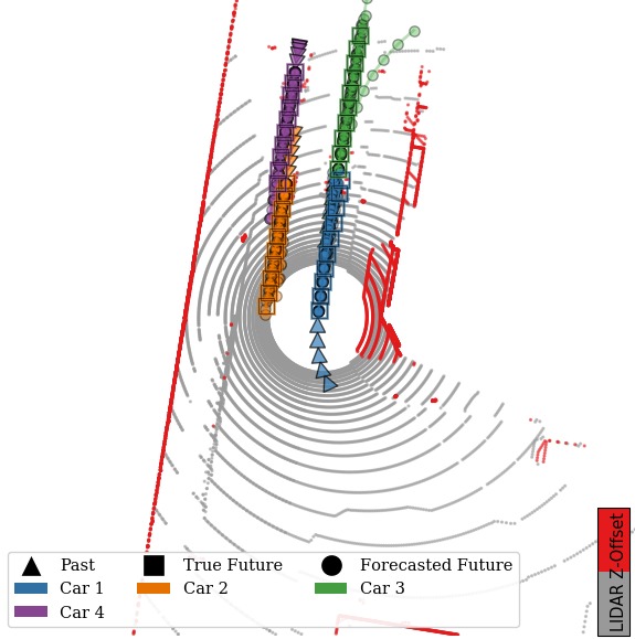
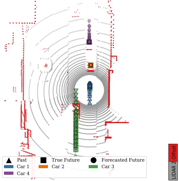
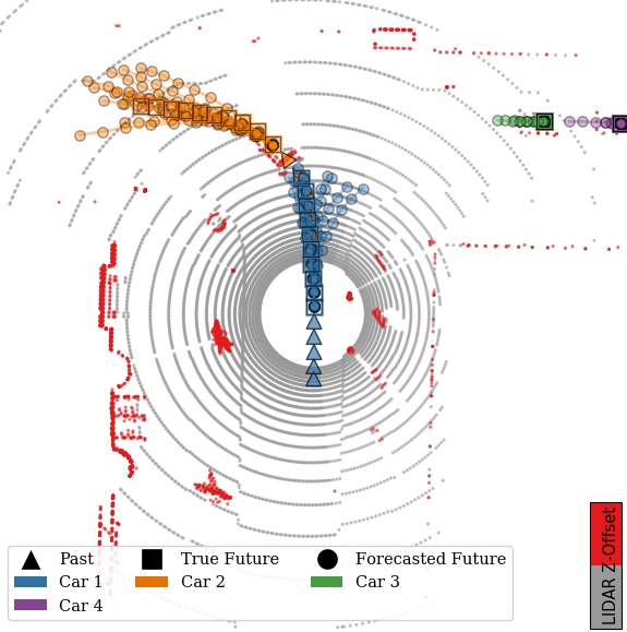
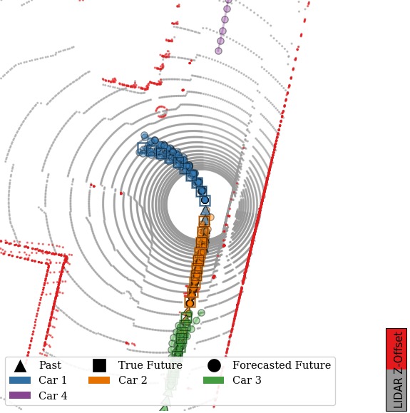
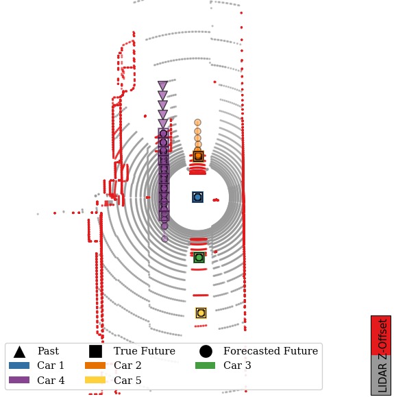
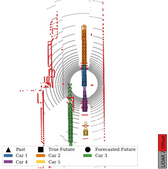
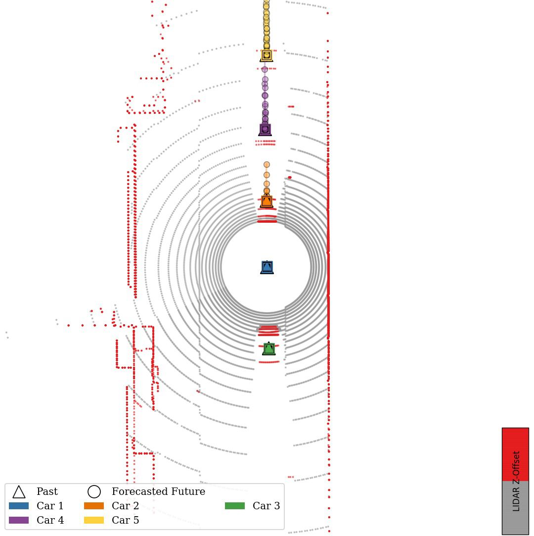
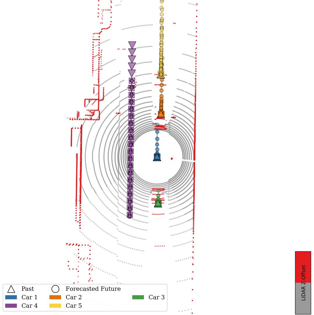
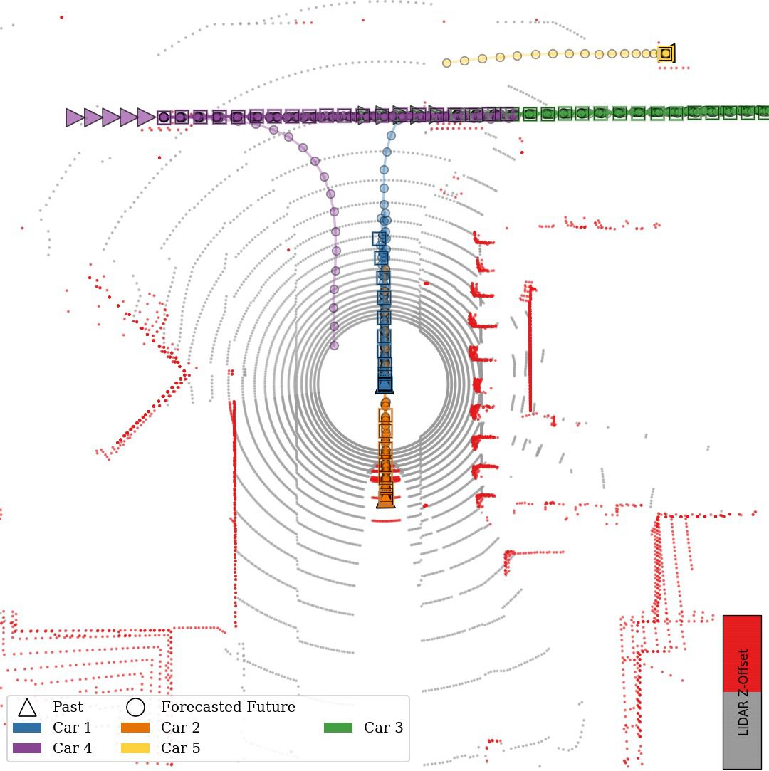
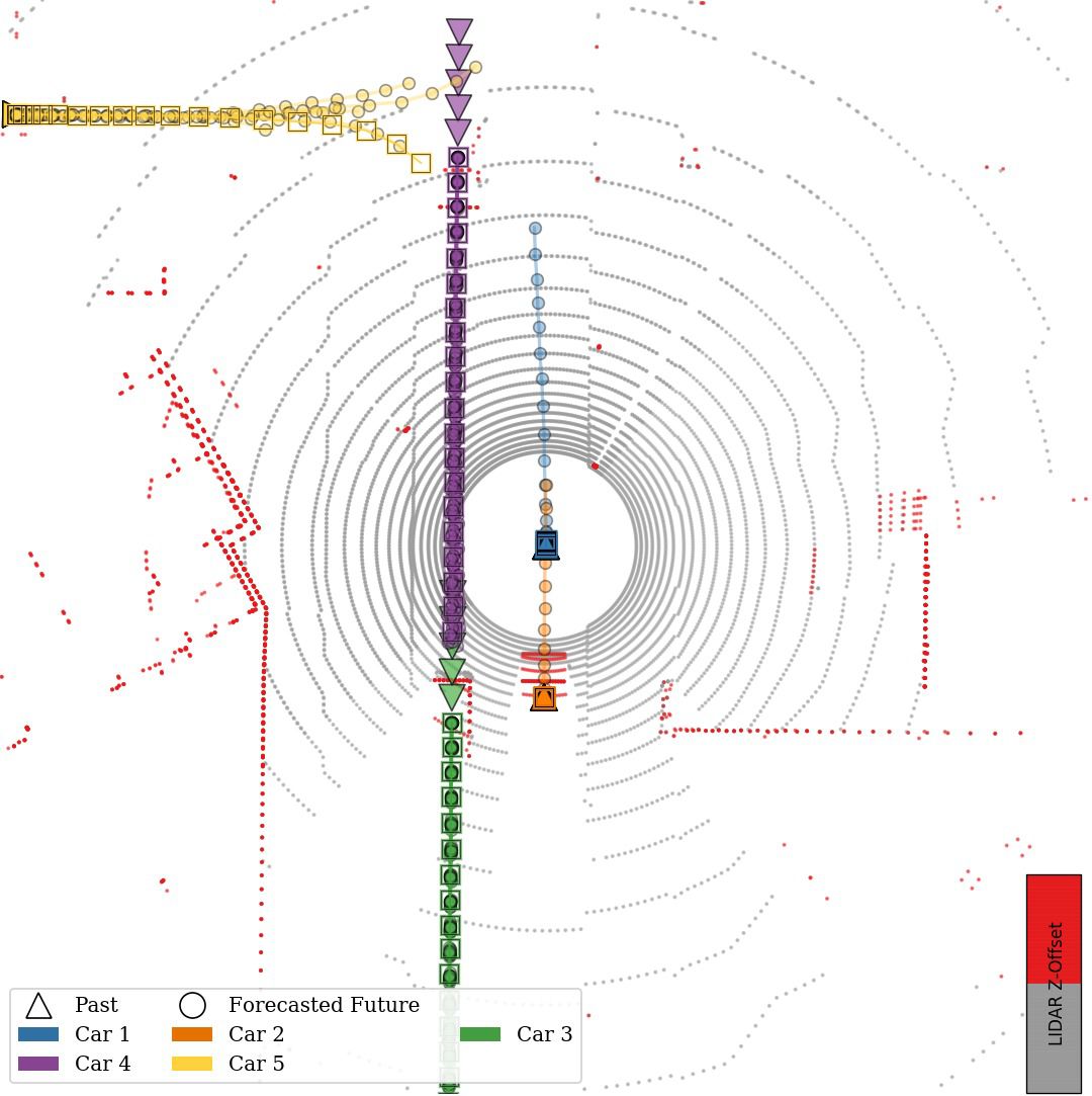
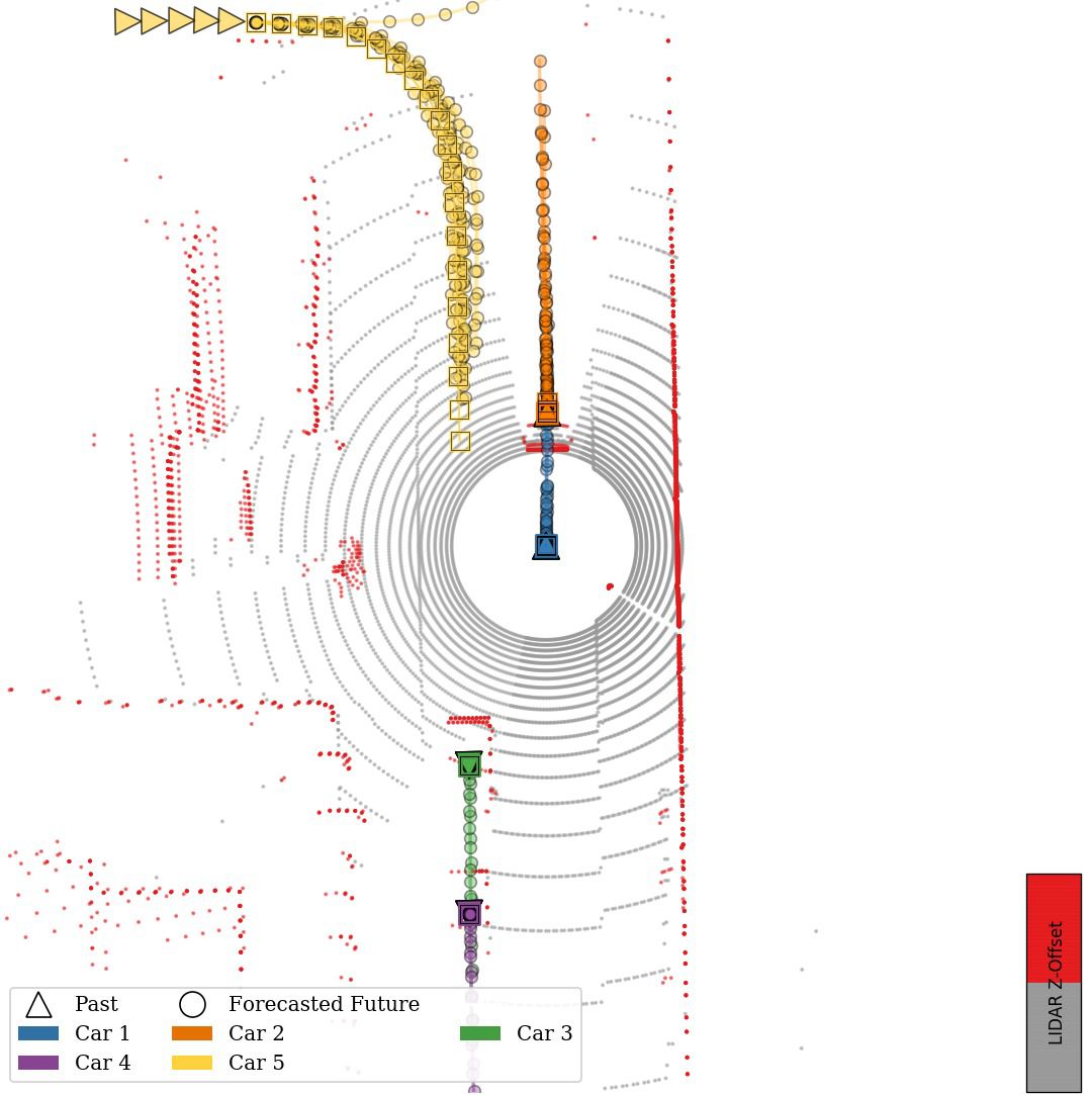
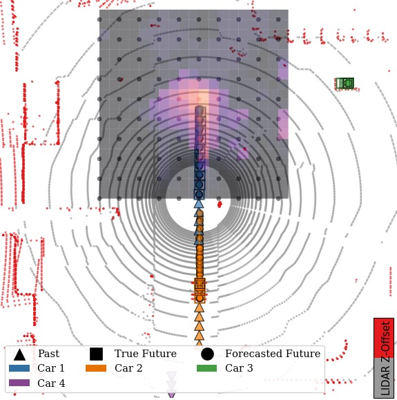
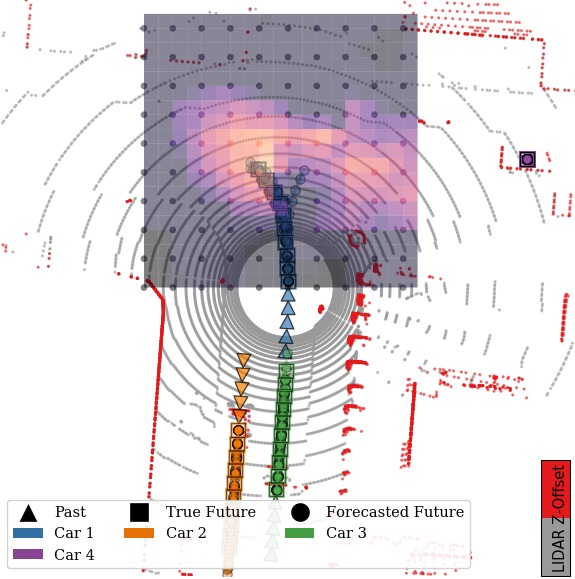
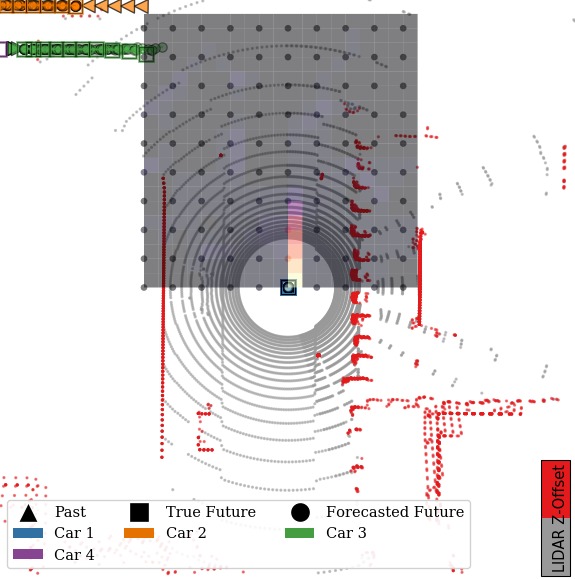
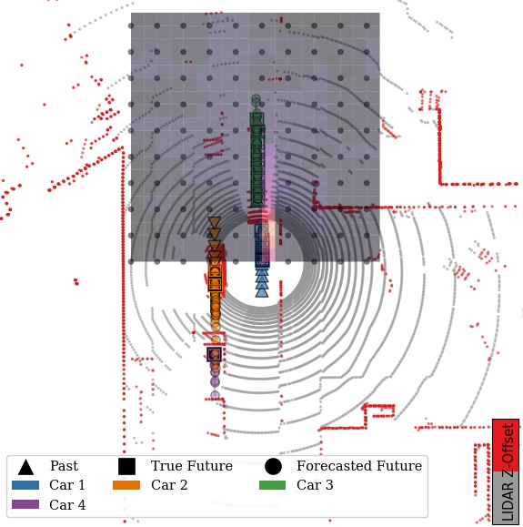
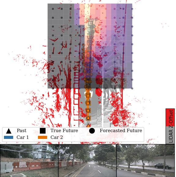
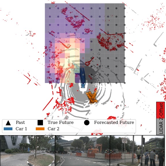
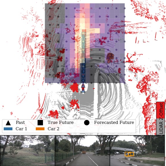
Qualitative examples of our forecasts are shown in Fig. 5. We observe three important types of multimodality: 1) multimodality in speed along a common specific direction, 2) the model properly predicts diverse plausible paths at intersections, and 3) when the agents are stopped, the model predicts sometimes the agents will stay still, and sometimes they will accelerate forward. The model also captures qualitative social behaviors, such as predicting that one car will wait for another before accelerating. See Appendix G for additional visualizations.

\begin{overpic}[width=496.85625pt]{fig/socialcross/asocial_control0.jpg} \put(1.0,88.0){{\hbox{\pagecolor{scrossgrey}{\color[rgb]{1,1,1}{ R2P2-MA\vphantom{g}}}}}} \end{overpic}
\begin{overpic}[width=496.85625pt]{fig/socialcross/asocial_control1.jpg} \put(1.0,88.0){{\hbox{\pagecolor{scrossgrey}{\color[rgb]{1,1,1}{ R2P2-MA\vphantom{g}}}}}} \end{overpic}
\begin{overpic}[width=496.85625pt]{fig/socialcross/social_control1.jpg} \put(1.0,88.0){{\hbox{\pagecolor{scrossgrey}{\color[rgb]{1,1,1}{ ESP\vphantom{g}}}}}} \end{overpic}
\begin{overpic}[width=496.85625pt]{fig/socialcross/social_control0.jpg} \put(1.0,88.0){{\hbox{\pagecolor{scrossgrey}{\color[rgb]{1,1,1}{ ESP\vphantom{g}}}}}} \end{overpic}
Model Test m^K=12subscript^𝑚𝐾12\hat{m}_{K=12} Test e^^𝑒\hat{e} Forecasting crashes Planning crashes
R2P2-MA 0.33130.33130.3313 0.0850.0850.085 50.8%percent50.850.8\% 49.5%percent49.549.5\%
ESP 0.00010.00010.0001 0.0310.0310.031 1.17%percent1.17{\bf{1.17}}\% 0.00%percent0.00{\bf{0.00}}\%
Figure 4: Didactic evaluation. Left plots: R2P2-MA cannot model agent interaction, and generates joint behaviors not present in the data. Right plots: ESP allows agents to influence each other, and does not generate undesirable joint behaviors.

Refer to caption
Refer to caption
\begin{overpic}[width=496.85625pt]{fig/nuscenes/a5/frame_00006_00000093_002.jpg} \put(0.0,15.5){{\hbox{\pagecolor{white}{\color[rgb]{0,0,0}{ Left\vphantom{g}}}}}} \put(33.0,15.5){{\hbox{\pagecolor{white}{\color[rgb]{0,0,0}{ Front\vphantom{g}}}}}} \put(66.0,15.5){{\hbox{\pagecolor{white}{\color[rgb]{0,0,0}{ Right}}}}} \end{overpic}
\begin{overpic}[width=496.85625pt]{fig/nuscenes/a5/frame_00007_00000125_002.jpg} \put(0.0,15.5){{\hbox{\pagecolor{white}{\color[rgb]{0,0,0}{ Left\vphantom{g}}}}}} \put(33.0,15.5){{\hbox{\pagecolor{white}{\color[rgb]{0,0,0}{ Front\vphantom{g}}}}}} \put(66.0,15.5){{\hbox{\pagecolor{white}{\color[rgb]{0,0,0}{ Right}}}}} \end{overpic}
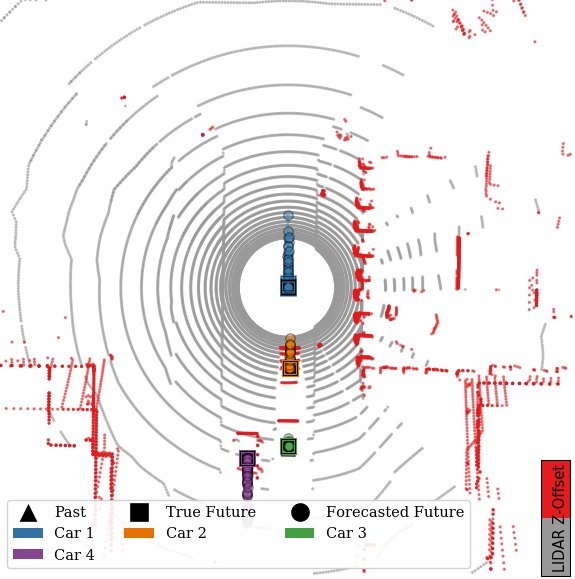
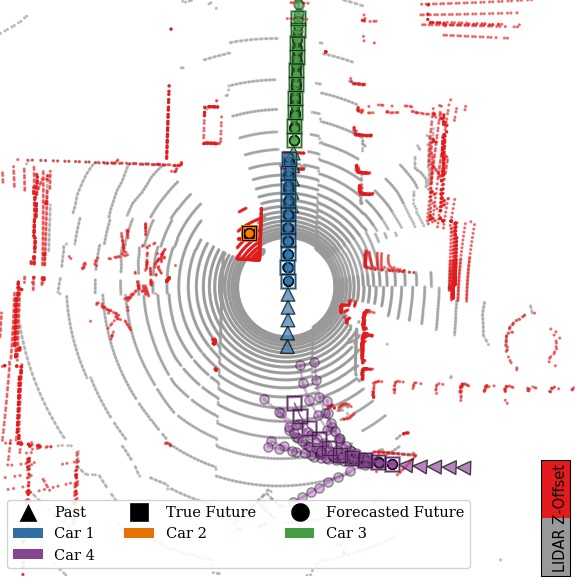
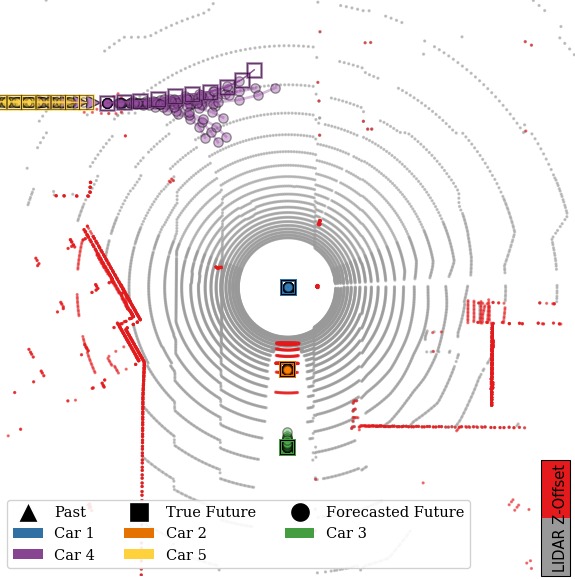
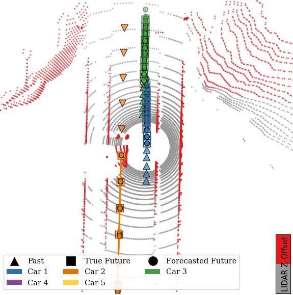
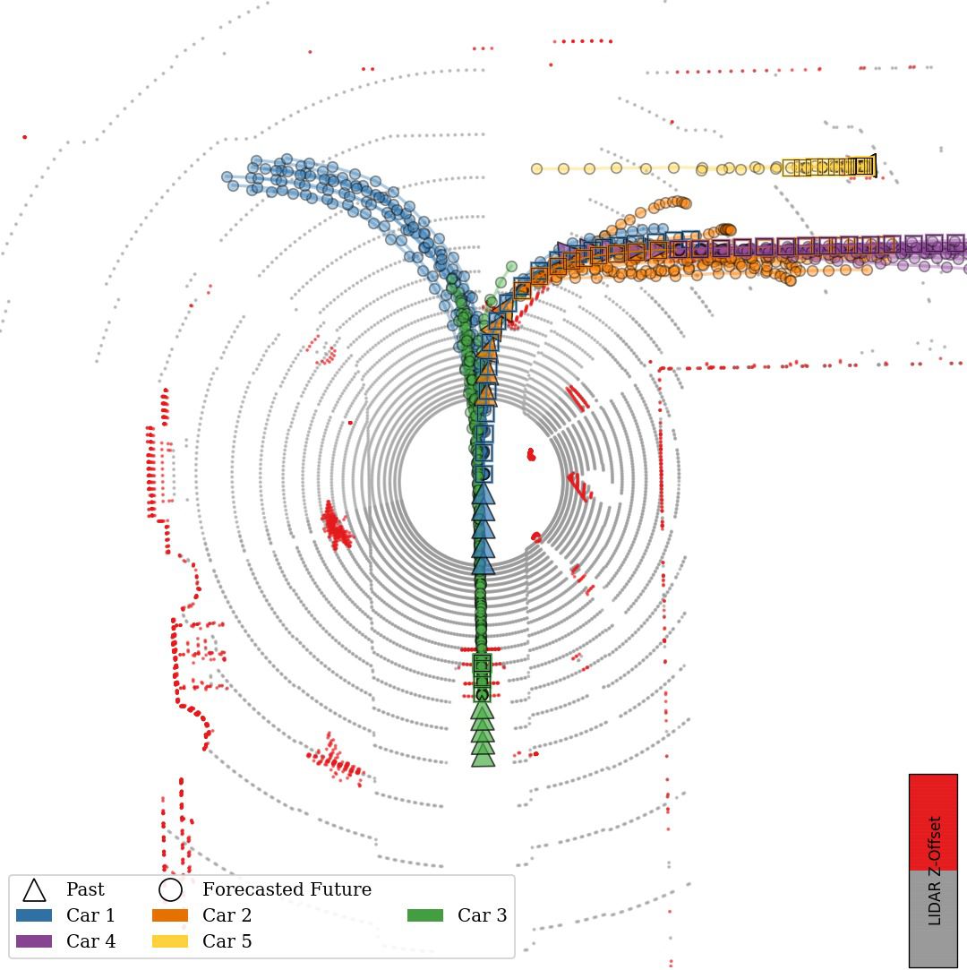
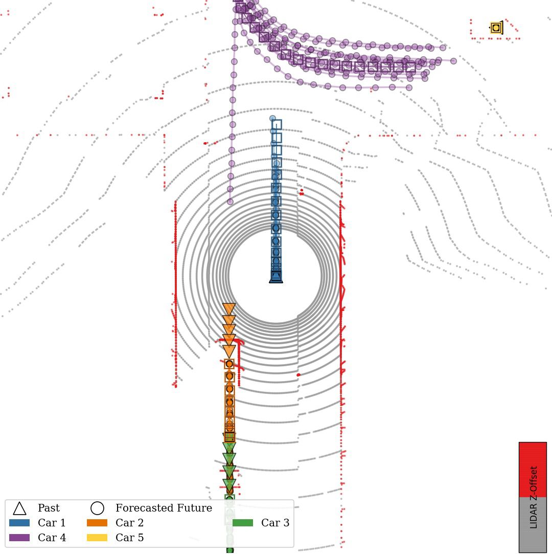
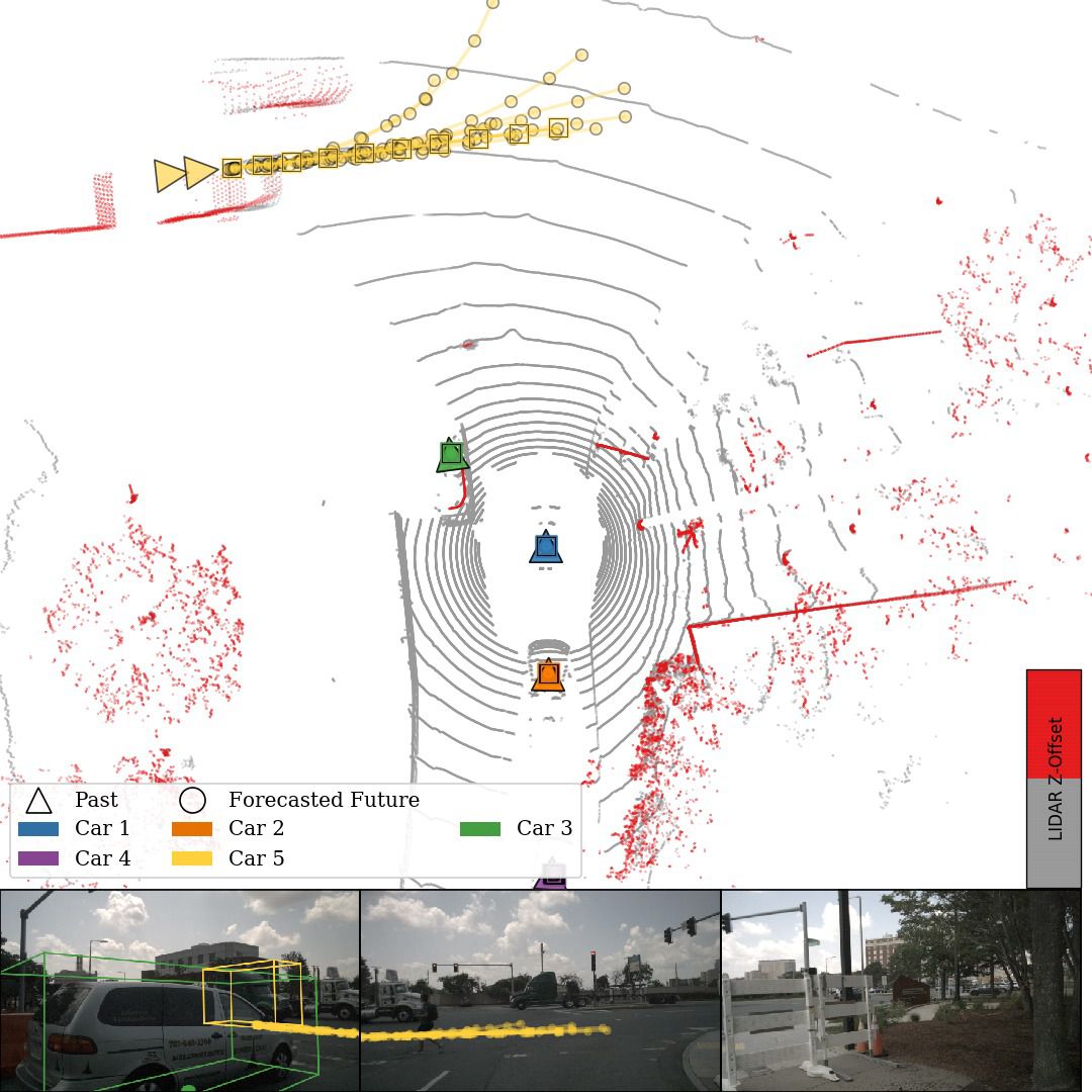
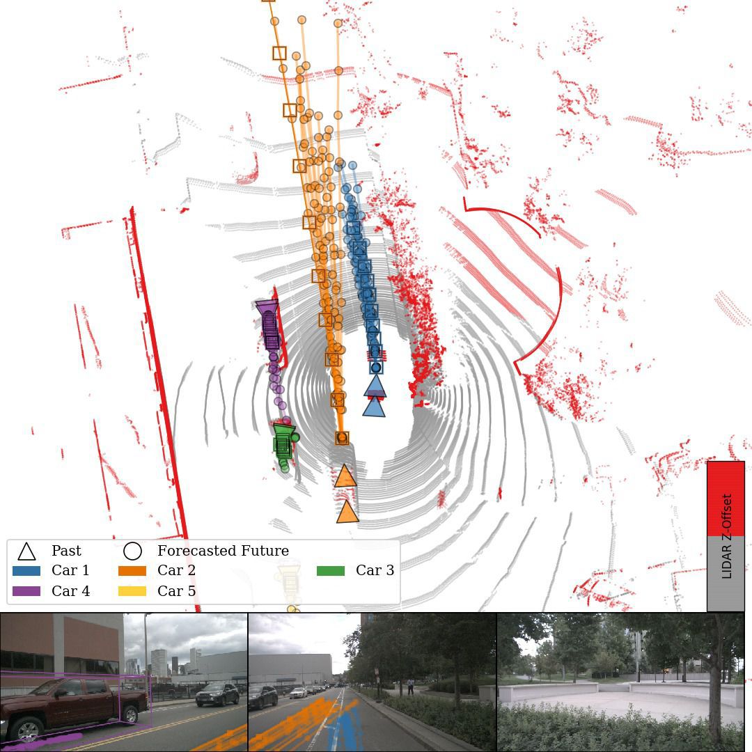
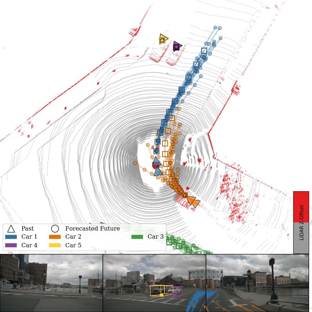
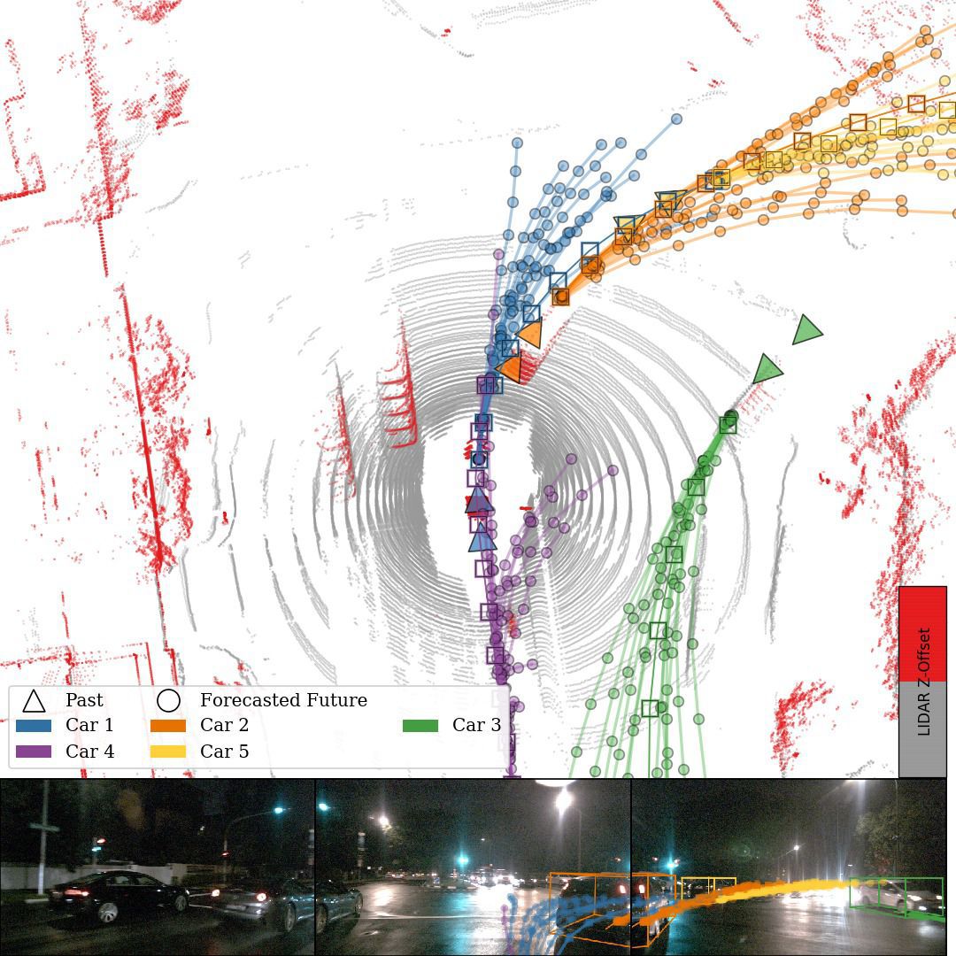
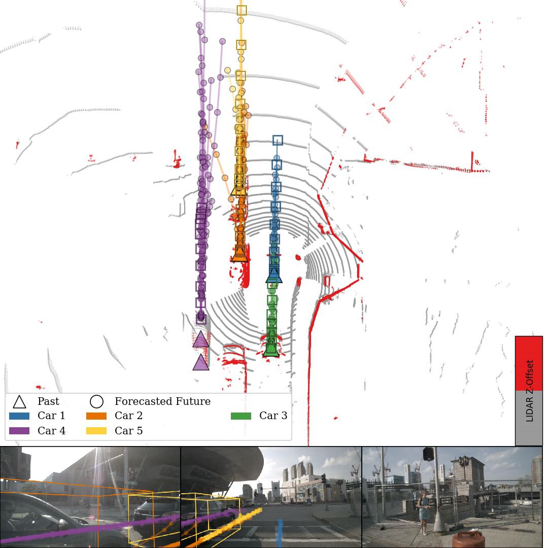
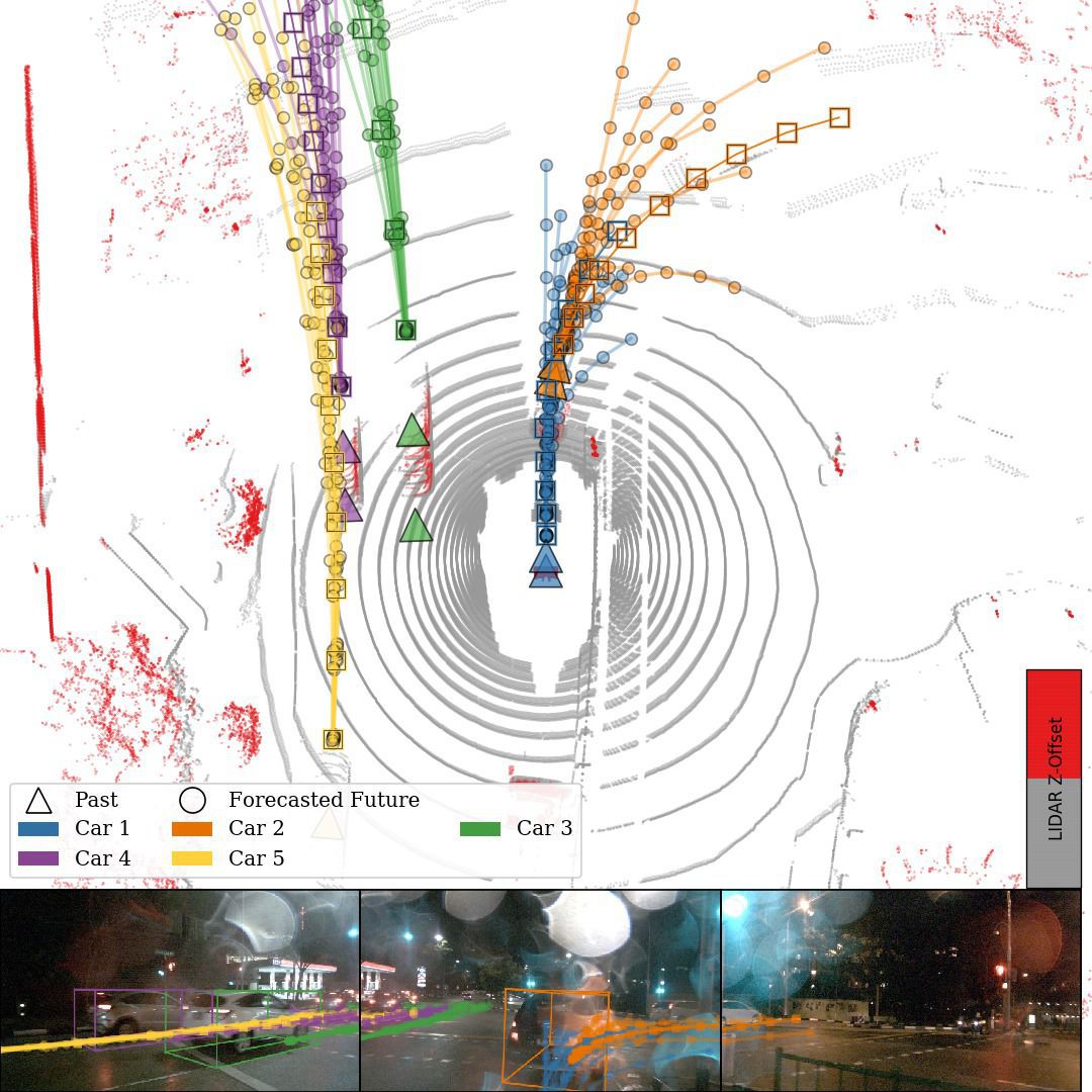
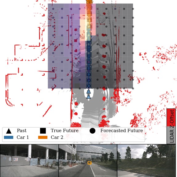
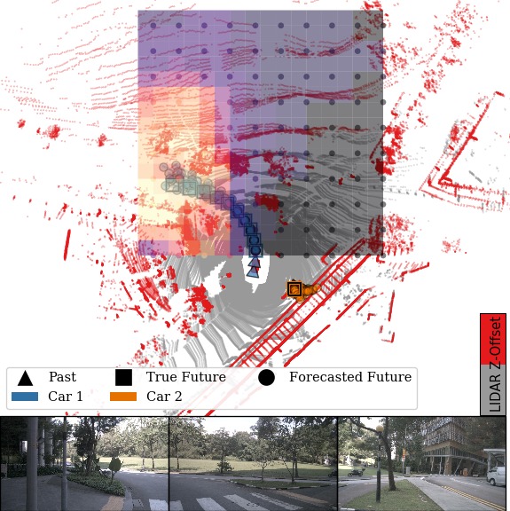
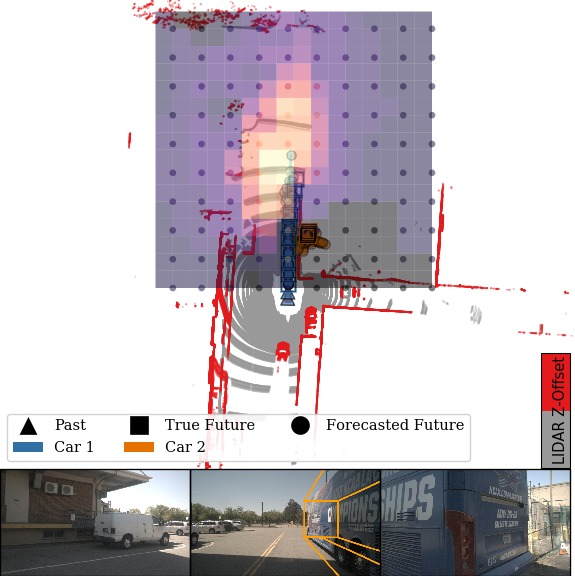
Figure 5: Examples of multi-agent forecasting with our learned ESP model. In each scene, 12 joint samples are shown, and LIDAR colors are discretized to near-ground and above-ground. Left: (CARLA) the model predicts Car 1 could either turn left or right, while the other agents’ future maintain multimodality in their speeds. Center-left: The model predicts Car 2 will likely wait (it is blocked by Cars 3 and 5), and that Cars 3 and 5 sometimes move forward together, and sometimes stay stationary. Center-right: Car 2 is predicted to overtake Car 1, which itself is forecasted to continue to wait for pedestrians and Car 2. Right: Car 4 is predicted to wait for the other cars to clear the intersection, and Car 5 is predicted to either start turning or continue straight.

4.4 PRECOG Experiments

Now we perform our second set of evaluations. We investigate if our planning approach enables us to sample more plausible joint futures of all agents. Unlike the previous unconditional forecasting scenario, when the robot is using the ESP model for planning, it knows its own goal. We can simulate planning offline by assuming the goal was the state that the robot actually reached at t=T𝑡𝑇t\!=\!T, and then planning a path from the current time step to this goal position. We can then evaluate the quality of the agent’s path and the stochastic paths of other agents under this plan. While this does not test our model in a full control scenario, it does allow us to evaluate whether conditioning on the goal provides more accurate and higher-confidence predictions. We use our model’s multi-agent prior (4) in the stochastic latent multi-agent planning objective (9), and define the goal-likelihood p(𝒢|𝐒,ϕ)=𝒩(𝐒Tr;𝐒Tr,0.1𝐈)𝑝conditional𝒢𝐒italic-ϕ𝒩subscriptsuperscript𝐒𝑟𝑇subscriptsuperscript𝐒absent𝑟𝑇0.1𝐈p(\mathcal{G}|\mathbf{S},\phi)\!=\!\mathcal{N}(\mathbf{S}^{r}_{T};\mathbf{S}^{*r}_{T},0.1\!\cdot\!\mathbf{I}), i.e. a normal distribution at the controlled agent’s last true future position, 𝐒Trsubscriptsuperscript𝐒absent𝑟𝑇\mathbf{S}^{*r}_{T}. As discussed, this knowledge might be available in control scenarios where we are confident we can achieve this positional goal. Other goal-likelihoods could be applied to relax this assumption, but this setup allows us to easily measure the quality of the resulting joint samples. We use gradient-descent on (9) to approximate 𝐳rsuperscript𝐳𝑟\mathbf{z}^{r*} (see supplement for details). The resulting latent plan yields highly likely joint trajectories under the uncertainty of other agents and approximately maximizes the goal-likelihood. Note that since we planned in latent space, the resulting robot trajectory is not fully determined – it can evolve differently depending on the stochasticity of the other agents. We next illustrate a scenario where joint modeling is critical to accurate forecasting and planning. Then, we conduct planning experiments on the CARLA and nuScenes datasets.

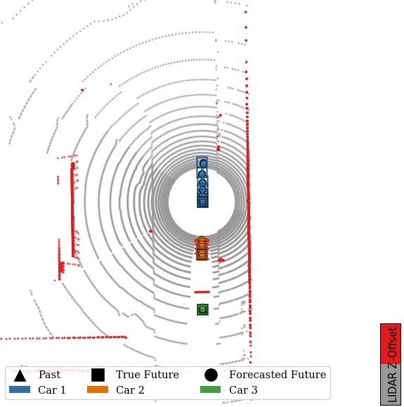
Figure 6: Forecasting evaluation of our model on CARLA Town01 Test and nuScenes Test data. Planning the robot to a goal position (PRECOG) generates better predictions for all agents. Means and their standard errors are reported. See Tab. 15 for all A={2..5}𝐴2..5A=\{2..5\}.
Data Approach Test m^K=12subscript^𝑚𝐾12\hat{m}_{K=12} Test m^K=12a=1superscriptsubscript^𝑚𝐾12𝑎1\hat{m}_{K=12}^{a=1} Test m^K=12a=2superscriptsubscript^𝑚𝐾12𝑎2\hat{m}_{K=12}^{a=2} Test m^K=12a=3superscriptsubscript^𝑚𝐾12𝑎3\hat{m}_{K=12}^{a=3} Test m^K=12a=4superscriptsubscript^𝑚𝐾12𝑎4\hat{m}_{K=12}^{a=4} Test m^K=12a=5superscriptsubscript^𝑚𝐾12𝑎5\hat{m}_{K=12}^{a=5}
CARLA  A=2𝐴2A\!=\!2 DESIRE [19] 1.83703±0.04810plus-or-minus1.837030.04810$1.83703$\pm$0.04810$ 1.99149±0.06605plus-or-minus1.991490.06605$1.99149$\pm$0.06605$ 1.68257±0.05013plus-or-minus1.682570.05013$1.68257$\pm$0.05013$
DESIRE-plan 1.85810±0.04614plus-or-minus1.858100.04614$1.85810$\pm$0.04614$ 0.91834±0.04441plus-or-minus0.918340.04441$0.91834$\pm$0.04441$ 2.79785±0.07331plus-or-minus2.797850.07331$2.79785$\pm$0.07331$
ESP 0.33705±0.0132plus-or-minus0.337050.0132$0.33705$\pm$0.0132$ 0.196±0.009plus-or-minus0.1960.009$0.196$\pm$0.009$ 0.478±0.024plus-or-minus0.4780.024$0.478$\pm$0.024$
PRECOG 0.2406397±0.01207plus-or-minus0.24063970.01207{\boldmath$0.2406397$\pm$0.01207$} 0.055±0.003plus-or-minus0.0550.003{\boldmath$0.055$\pm$0.003$} 0.426±0.024plus-or-minus0.4260.024{\boldmath$0.426$\pm$0.024$}
CARLA  A=5𝐴5A\!=\!5 DESIRE [19] 2.62247±0.02953plus-or-minus2.622470.02953$2.62247$\pm$0.02953$ 2.62066±0.04547plus-or-minus2.620660.04547$2.62066$\pm$0.04547$ 2.42165±0.04842plus-or-minus2.421650.04842$2.42165$\pm$0.04842$ 2.71018±0.06613plus-or-minus2.710180.06613$2.71018$\pm$0.06613$ 2.96901±0.05700plus-or-minus2.969010.05700$2.96901$\pm$0.05700$ 2.39086±0.04891plus-or-minus2.390860.04891$2.39086$\pm$0.04891$
DESIRE-plan 2.32850±0.03837plus-or-minus2.328500.03837$2.32850$\pm$0.03837$ 0.19446±0.00359plus-or-minus0.194460.00359$0.19446$\pm$0.00359$ 2.23880±0.05707plus-or-minus2.238800.05707$2.23880$\pm$0.05707$ 3.11885±0.09775plus-or-minus3.118850.09775$3.11885$\pm$0.09775$ 3.33222±0.09021plus-or-minus3.332220.09021$3.33222$\pm$0.09021$ 2.75818±0.08278plus-or-minus2.758180.08278$2.75818$\pm$0.08278$
ESP 0.71759±0.01187plus-or-minus0.717590.01187$0.71759$\pm$0.01187$ 0.34031±0.01146plus-or-minus0.340310.01146$0.34031$\pm$0.01146$ 0.75908±0.02449plus-or-minus0.759080.02449$0.75908$\pm$0.02449$ 0.80909±0.02504plus-or-minus0.809090.02504$0.80909$\pm$0.02504$ 0.85122±0.02335plus-or-minus0.851220.02335$0.85122$\pm$0.02335$ 0.82827±0.02411plus-or-minus0.828270.02411$0.82827$\pm$0.02411$
PRECOG 0.64039±0.01109plus-or-minus0.640390.01109{\boldmath$0.64039$\pm$0.01109$} 0.06557±0.00348plus-or-minus0.065570.00348{\boldmath$0.06557$\pm$0.00348$} 0.74088±0.02363plus-or-minus0.740880.02363{\boldmath$0.74088$\pm$0.02363$} 0.79019±0.02449plus-or-minus0.790190.02449{\boldmath$0.79019$\pm$0.02449$} 0.80444±0.02238plus-or-minus0.804440.02238{\boldmath$0.80444$\pm$0.02238$} 0.80085±0.02401plus-or-minus0.800850.02401{\boldmath$0.80085$\pm$0.02401$}
nuScenes  A=2𝐴2A\!=\!2 DESIRE [19] 3.30741±0.09280plus-or-minus3.307410.09280$3.30741$\pm$0.09280$ 3.00155±0.08819plus-or-minus3.001550.08819$3.00155$\pm$0.08819$ 3.61328±0.13969plus-or-minus3.613280.13969$3.61328$\pm$0.13969$
DESIRE-plan 4.52804±0.15055plus-or-minus4.528040.15055$4.52804$\pm$0.15055$ 0.45641±0.01544plus-or-minus0.456410.01544$0.45641$\pm$0.01544$ 8.59966±0.29765plus-or-minus8.599660.29765$8.59966$\pm$0.29765$
ESP 1.09373±0.05281plus-or-minus1.093730.05281$1.09373$\pm$0.05281$ 0.95464±0.05651plus-or-minus0.954640.05651$0.95464$\pm$0.05651$ 1.23282±0.07814plus-or-minus1.232820.07814$1.23282$\pm$0.07814$
PRECOG 0.51431±0.03667plus-or-minus0.514310.03667\boldmath$0.51431$\pm$0.03667$ 0.15778±0.01621plus-or-minus0.157780.01621\boldmath$0.15778$\pm$0.01621$ 0.87085±0.07002plus-or-minus0.870850.07002\boldmath$0.87085$\pm$0.07002$
nuScenes  A=5𝐴5A\!=\!5 DESIRE [19] 6.82986±0.20435plus-or-minus6.829860.20435$6.82986$\pm$0.20435$ 4.99886±0.21870plus-or-minus4.998860.21870$4.99886$\pm$0.21870$ 6.41475±0.29442plus-or-minus6.414750.29442$6.41475$\pm$0.29442$ 7.02696±0.36014plus-or-minus7.026960.36014$7.02696$\pm$0.36014$ 7.41826±0.32365plus-or-minus7.418260.32365$7.41826$\pm$0.32365$ 8.29048±0.53172plus-or-minus8.290480.53172$8.29048$\pm$0.53172$
DESIRE-plan 6.56219±0.20719plus-or-minus6.562190.20719$6.56219$\pm$0.20719$ 2.26053±0.09984plus-or-minus2.260530.09984$2.26053$\pm$0.09984$ 6.64410±0.31435plus-or-minus6.644100.31435$6.64410$\pm$0.31435$ 6.18376±0.32513plus-or-minus6.183760.32513$6.18376$\pm$0.32513$ 9.20305±0.44800plus-or-minus9.203050.44800$9.20305$\pm$0.44800$ 8.51950±0.51390plus-or-minus8.519500.51390$8.51950$\pm$0.51390$
ESP 2.92126±0.17499plus-or-minus2.921260.17499$2.92126$\pm$0.17499$ 1.86066±0.10935plus-or-minus1.860660.10935$1.86066$\pm$0.10935$ 2.36853±0.18780plus-or-minus2.368530.18780$2.36853$\pm$0.18780$ 2.81241±0.18794plus-or-minus2.812410.18794$2.81241$\pm$0.18794$ 3.20137±0.25363plus-or-minus3.201370.25363$3.20137$\pm$0.25363$ 4.36335±0.65235plus-or-minus4.363350.65235$4.36335$\pm$0.65235$
PRECOG 2.50763±0.15214plus-or-minus2.507630.15214\boldmath$2.50763$\pm$0.15214$ 0.14913±0.02075plus-or-minus0.149130.02075\boldmath$0.14913$\pm$0.02075$ 2.32361±0.18743plus-or-minus2.323610.18743\boldmath$2.32361$\pm$0.18743$ 2.65441±0.19017plus-or-minus2.654410.19017\boldmath$2.65441$\pm$0.19017$ 3.15719±0.27262plus-or-minus3.157190.27262\boldmath$3.15719$\pm$0.27262$ 4.25379±0.58602plus-or-minus4.253790.58602\boldmath$4.25379$\pm$0.58602$
Refer to caption
(a) CARLA, ESP
Refer to caption
(b) CARLA, PRECOG
Refer to caption
(c) nuScenes, ESP
Refer to caption
(d) nuScenes, PRECOG
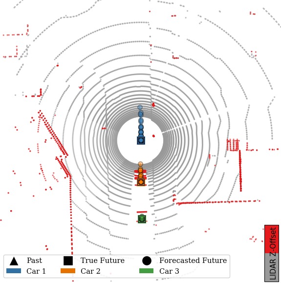
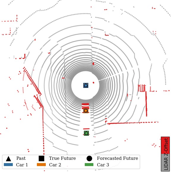
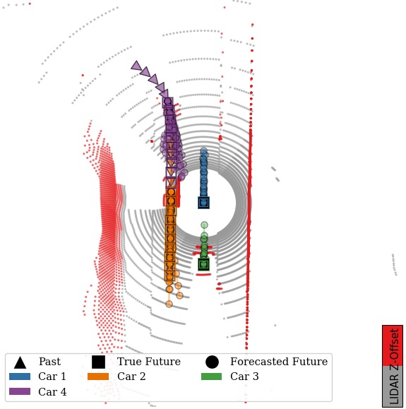
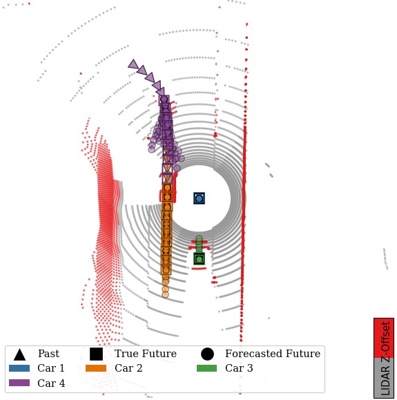
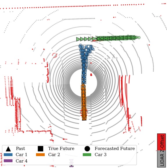
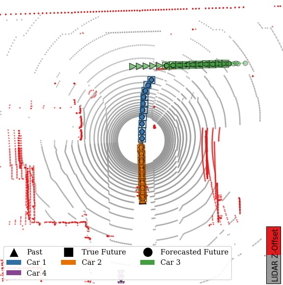
Figure 7: Examples of planned multi-agent forecasting (PRECOG) with our learned model in CARLA and nuScenes. By using our planning approach and conditioning the robot on its true final position, our predictions of the other agents change, our predictions for the robot become more accurate, and sometimes our predictions of the other agent become more accurate.

4.4.1 CARLA and nuScenes PRECOG

DESIRE planning baseline: We developed a straightforward planning baseline by feeding an input goal state and past encoding to a two-layer 200-unit ReLU MLP trained to predict the latent state of the robot given training tuples (x=(X,𝐒TrqDESIRE(𝐒|ϕ,𝐳r)T)),y=𝐳r)(x\!=\!(\!\mathcal{H}_{X},\mathbf{S}^{r}_{T}\sim\!q_{\text{DESIRE}}(\mathbf{S}|\phi,\mathbf{z}^{r})_{T})),y=\mathbf{z}^{r}). The latents for the other agents are samples from their DESIRE priors.

Experiments: We use the trained ESP models to run PRECOG on the test-sets in CARLA and nuScenes. Here, we use both m^Ksubscript^𝑚𝐾\hat{m}_{K} and m^Kasuperscriptsubscript^𝑚𝐾𝑎\hat{m}_{K}^{a} to quantify joint sample quality in terms of all agents and each agent individually. In Tab. 6 and Fig. 7, we report results of our planning experiments. We observe that our planning approach significantly improves the quality of the joint trajectories. As expected, the forecasting performance improves the most for the planned agent (m^K1superscriptsubscript^𝑚𝐾1\hat{m}_{K}^{1}). Notably, the forecasting performance of the other agents improves across all datasets and all agents. We see the non-planned-agent improvements are usually greatest for Car 2 (m^K2superscriptsubscript^𝑚𝐾2\hat{m}_{K}^{2}). This result conforms to our intuitions: Car 2 is the closest agent to the planned agent, and thus, it the agent that Car 1 influences the most. Qualitative examples of this planning are shown in Fig. 7. We observe trends similar to the CARLA planning experiments – the forecasting performance improves the most for the planned agent, with the forecasting performance of the unplanned agent improving in response to the latent plans. See Appendix G for additional visualizations.

5 Conclusions

We present a multi-agent forecasting method, ESP, that outperforms state-of-the-art multi-agent forecasting methods on real (nuScenes) and simulated (CARLA) driving data. We also developed a novel algorithm, PRECOG, to condition forecasts on agent goals. We showed conditional forecasts improve joint-agent and per-agent predictions, compared to unconditional forecasts used in prior work. Conditional forecasting can be used for planning, which we demonstrated with a novel multi-agent imitative planning objective. Future directions include conditional forecasting w.r.t. multiple agent goals, useful for multi-AV coordination via communicated intent.

Acknowledgements: We thank K. Rakelly, A. Filos, A. Del Giorno, A. Dragan, and reviewers for their helpful feedback. Sponsored in part by IARPA (D17PC00340), ARL DCIST CRA W911NF-17-2-0181, DARPA via the Assured Autonomy Program, the ONR, and NVIDIA.

References

  • [1] Alexandre Alahi, Kratarth Goel, Vignesh Ramanathan, Alexandre Robicquet, Li Fei-Fei, and Silvio Savarese. Social LSTM: Human trajectory prediction in crowded spaces. In Computer Vision and Pattern Recognition (CVPR), June 2016.
  • [2] David Barber. Bayesian reasoning and machine learning. Cambridge University Press, 2012.
  • [3] Federico Bartoli, Giuseppe Lisanti, Lamberto Ballan, and Alberto Del Bimbo. Context-aware trajectory prediction. arXiv preprint arXiv:1705.02503, 2017.
  • [4] Holger Caesar, Varun Bankiti, Alex H. Lang, Sourabh Vora, Venice Erin Liong, Qiang Xu, Anush Krishnan, Yu Pan, Giancarlo Baldan, and Oscar Beijbom. nuscenes: A multimodal dataset for autonomous driving. arXiv preprint arXiv:1903.11027, 2019.
  • [5] Caroline Claus and Craig Boutilier. The dynamics of reinforcement learning in cooperative multiagent systems. AAAI/IAAI, 1998:746–752, 1998.
  • [6] Nachiket Deo and Mohan M Trivedi. Multi-modal trajectory prediction of surrounding vehicles with maneuver based LSTMs. arXiv preprint arXiv:1805.05499, 2018.
  • [7] Laurent Dinh, Jascha Sohl-Dickstein, and Samy Bengio. Density estimation using Real NVP. arXiv preprint arXiv:1605.08803, 2016.
  • [8] Alexey Dosovitskiy, German Ros, Felipe Codevilla, Antonio Lopez, and Vladlen Koltun. CARLA: An open urban driving simulator. In Conference on Robot Learning (CoRL), pages 1–16, 2017.
  • [9] Panna Felsen, Patrick Lucey, and Sujoy Ganguly. Where will they go? Predicting fine-grained adversarial multi-agent motion using conditional variational autoencoders. In Proceedings of the European Conference on Computer Vision (ECCV), pages 732–747, 2018.
  • [10] Tharindu Fernando, Simon Denman, Sridha Sridharan, and Clinton Fookes. Soft + hardwired attention: An LSTM framework for human trajectory prediction and abnormal event detection. Neural networks, 108:466–478, 2018.
  • [11] Jaime F Fisac, Eli Bronstein, Elis Stefansson, Dorsa Sadigh, S Shankar Sastry, and Anca D Dragan. Hierarchical game-theoretic planning for autonomous vehicles. arXiv preprint arXiv:1810.05766, 2018.
  • [12] Will Grathwohl, Ricky TQ Chen, Jesse Betterncourt, Ilya Sutskever, and David Duvenaud. FFJORD: Free-form continuous dynamics for scalable reversible generative models. arXiv preprint arXiv:1810.01367, 2018.
  • [13] Jiaqi Guan, Ye Yuan, Kris M Kitani, and Nicholas Rhinehart. Generative hybrid representations for activity forecasting with no-regret learning. arXiv preprint arXiv:1904.06250, 2019.
  • [14] Agrim Gupta, Justin Johnson, Li Fei-Fei, Silvio Savarese, and Alexandre Alahi. Social GAN: Socially acceptable trajectories with generative adversarial networks. In Computer Vision and Pattern Recognition (CVPR), 2018.
  • [15] Boris Ivanovic, Edward Schmerling, Karen Leung, and Marco Pavone. Generative modeling of multimodal multi-human behavior. arXiv preprint arXiv:1803.02015, 2018.
  • [16] Durk P Kingma and Prafulla Dhariwal. Glow: Generative flow with invertible 1x1 convolutions. In Advances in Neural Information Processing Systems, pages 10236–10245, 2018.
  • [17] Diederik P Kingma and Max Welling. Auto-encoding variational Bayes. arXiv preprint arXiv:1312.6114, 2013.
  • [18] Hoang M Le, Yisong Yue, Peter Carr, and Patrick Lucey. Coordinated multi-agent imitation learning. In International Conference on Machine Learning, pages 1995–2003, 2017.
  • [19] Namhoon Lee, Wongun Choi, Paul Vernaza, Christopher B Choy, Philip HS Torr, and Manmohan Chandraker. DESIRE: Distant future prediction in dynamic scenes with interacting agents. In Computer Vision and Pattern Recognition (CVPR), pages 336–345, 2017.
  • [20] Namhoon Lee and Kris M Kitani. Predicting wide receiver trajectories in american football. In 2016 IEEE Winter Conference on Applications of Computer Vision (WACV), pages 1–9. IEEE, 2016.
  • [21] Wei-Chiu Ma, De-An Huang, Namhoon Lee, and Kris M Kitani. Forecasting interactive dynamics of pedestrians with fictitious play. In Computer Vision and Pattern Recognition (CVPR), pages 4636–4644. IEEE, 2017.
  • [22] Rowan McAllister, Yarin Gal, Alex Kendall, Mark Van Der Wilk, Amar Shah, Roberto Cipolla, and Adrian Vivian Weller. Concrete problems for autonomous vehicle safety: Advantages of Bayesian deep learning. In International Joint Conferences on Artificial Intelligence (IJCAI), 2017.
  • [23] Robert J McCann et al. Existence and uniqueness of monotone measure-preserving maps. Duke Mathematical Journal, 1995.
  • [24] Francisco S Melo and Manuela Veloso. Decentralized MDPs with sparse interactions. Artificial Intelligence, 175(11):1757–1789, 2011.
  • [25] Takayuki Osa, Joni Pajarinen, Gerhard Neumann, J Andrew Bagnell, Pieter Abbeel, Jan Peters, et al. An algorithmic perspective on imitation learning. Foundations and Trends® in Robotics, 7(1-2):1–179, 2018.
  • [26] SeongHyeon Park, ByeongDo Kim, Chang Mook Kang, Chung Choo Chung, and Jun Won Choi. Sequence-to-sequence prediction of vehicle trajectory via LSTM encoder-decoder architecture. arXiv preprint arXiv:1802.06338, 2018.
  • [27] Emanuel Parzen. On estimation of a probability density function and mode. The annals of mathematical statistics, 33(3):1065–1076, 1962.
  • [28] Stefano Pellegrini, Andreas Ess, Konrad Schindler, and Luc Van Gool. You’ll never walk alone: Modeling social behavior for multi-target tracking. In Computer Vision, 2009 IEEE 12th International Conference on, pages 261–268. IEEE, 2009.
  • [29] Dean A Pomerleau. Alvinn: An autonomous land vehicle in a neural network. In Advances in neural information processing systems, pages 305–313, 1989.
  • [30] Nicholas Rhinehart, Kris M. Kitani, and Paul Vernaza. R2P2: A reparameterized pushforward policy for diverse, precise generative path forecasting. In European Conference on Computer Vision (ECCV), September 2018.
  • [31] Nicholas Rhinehart, Rowan McAllister, and Sergey Levine. Deep imitative models for flexible inference, planning, and control. arXiv preprint arXiv:1810.06544, 2018.
  • [32] Murray Rosenblatt. Remarks on some nonparametric estimates of a density function. The Annals of Mathematical Statistics, pages 832–837, 1956.
  • [33] Edward Schmerling, Karen Leung, Wolf Vollprecht, and Marco Pavone. Multimodal probabilistic model-based planning for human-robot interaction. In International Conference on Robotics and Automation (ICRA), pages 1–9. IEEE, 2018.
  • [34] Chen Sun, Per Karlsson, Jiajun Wu, Joshua B Tenenbaum, and Kevin Murphy. Stochastic prediction of multi-agent interactions from partial observations. arXiv preprint arXiv:1902.09641, 2019.
  • [35] Ming Tan. Multi-agent reinforcement learning: Independent vs. cooperative agents. In Proceedings of the tenth international conference on machine learning, pages 330–337, 1993.
  • [36] Eric Zhan, Stephan Zheng, Yisong Yue, and Patrick Lucey. Generative multi-agent behavioral cloning. arXiv preprint arXiv:1803.07612, 2018.
  • [37] Tianyang Zhao, Yifei Xu, Mathew Monfort, Wongun Choi, Chris Baker, Yibiao Zhao, Yizhou Wang, and Ying Nian Wu. Multi-agent tensor fusion for contextual trajectory prediction. arXiv preprint arXiv:1904.04776, 2019.

Appendix A Planning and Forecasting Algorithms

To execute planning, we perform gradient ascent to approximately solve the optimization problem (10). Recall the latent joint behavior is 𝐙𝐙1:T1:Aapproaches-limit𝐙subscriptsuperscript𝐙:1𝐴:1𝑇\mathbf{Z}\doteq\mathbf{Z}^{1:A}_{1:T}, the latent human behavior is 𝐙h𝐙1:T2:Aapproaches-limitsuperscript𝐙subscriptsuperscript𝐙:2𝐴:1𝑇\mathbf{Z}^{h}\doteq\mathbf{Z}^{2:A}_{1:T}, and the robot behavior is 𝐳r𝐳1:T1approaches-limitsuperscript𝐳𝑟subscriptsuperscript𝐳1:1𝑇\mathbf{z}^{r}\doteq\mathbf{z}^{1}_{1:T}. We approximate the expectation in (9) with a sample expectation over K𝐾K samples from p(𝐙h)=𝒩(𝟎,𝐈)𝑝superscript𝐙𝒩0𝐈p(\mathbf{Z}^{h})=\mathcal{N}(\mathbf{0},\mathbf{I}), denoted 𝐳h1:Ksuperscriptsuperscript𝐳:1𝐾{}^{1:K}\!\mathbf{z}^{h}, where the kthsuperscript𝑘thk^{\mathrm{th}} sample is 𝐳hksuperscriptsuperscript𝐳𝑘{}^{k}\!\mathbf{z}^{h}. Each of these samples for the latent human behavior is combined with the single latent robot plan, each denoted 𝐳k=[𝐳r,𝐳hk]superscript𝐳𝑘superscript𝐳𝑟superscriptsuperscript𝐳𝑘{}^{k}\!\mathbf{z}=[\mathbf{z}^{r},{}^{k}\!\mathbf{z}^{h}]. This batch is denoted 𝐳1:Ksuperscript𝐳:1𝐾{}^{1:K}\!\mathbf{z}. The approximation of (9) is then given as

L^(𝐳1:K,𝒢,ϕ)=1Kk=1K^𝐿superscript𝐳:1𝐾𝒢italic-ϕ1𝐾superscriptsubscript𝑘1𝐾\displaystyle\!\hat{L}({}^{1:K}\!\mathbf{z},\mathcal{G},\!\phi)\!=\!\frac{1}{K}\sum_{k=1}^{K}\! log(q(f(𝐳k)|ϕ)p(𝒢|f(𝐳k),ϕ)),𝑞conditional𝑓superscript𝐳𝑘italic-ϕ𝑝conditional𝒢𝑓superscript𝐳𝑘italic-ϕ\displaystyle\log(q(f({}^{k}\!{\mathbf{z}})|\phi)p(\mathcal{G}|f({}^{k}\!{\mathbf{z}}),\phi)), (14)

with L^^𝐿\hat{L} parameterized by (q,f,p)𝑞𝑓𝑝(q,f,p), and f𝑓f’s dependence on ϕitalic-ϕ\phi dropped for notational brevity. The 𝐳h1:Ksuperscriptsuperscript𝐳:1𝐾{}^{1:K}\!\mathbf{z}^{h} is redrawn before each gradient ascent step on (14). This procedure is illustrated in Alg. 1.

Algorithm 1 MultiImitativePlan(q,f,p,ϕ,K𝑞𝑓𝑝italic-ϕ𝐾q,f,p,\phi,K)
1:  Define L^^𝐿\hat{L} with q,f,p𝑞𝑓𝑝q,f,p
2:  Initialize 𝐳1:Tr𝒩(0,I)similar-tosuperscriptsubscript𝐳:1𝑇𝑟𝒩0𝐼\mathbf{z}_{1:T}^{r}\sim\mathcal{N}(0,I)
3:  while not converged do
4:     𝐳h1:KiidN(0,I)superscriptsimilar-toiidsuperscriptsuperscript𝐳:1𝐾𝑁0𝐼{}^{1:K}\!{\mathbf{z}}^{h}\stackrel{{\scriptstyle\mathclap{\mathrm{iid}}}}{{\sim}}N(0,I)
5:     𝐳1:Tr𝐳1:Tr+𝐳1:TrL^(𝐳1:K,𝒢,ϕ)superscriptsubscript𝐳:1𝑇𝑟superscriptsubscript𝐳:1𝑇𝑟subscriptsuperscriptsubscript𝐳:1𝑇𝑟^𝐿superscript𝐳:1𝐾𝒢italic-ϕ\mathbf{z}_{1:T}^{r}\leftarrow\mathbf{z}_{1:T}^{r}+\nabla_{\mathbf{z}_{1:T}^{r}}\hat{L}({}^{1:K}\!\mathbf{z},\mathcal{G},\phi)
6:  end while
7:  return 𝐳1:Trsuperscriptsubscript𝐳:1𝑇𝑟\mathbf{z}_{1:T}^{r}

In our implementation, we use K=12𝐾12K\!=\!12, track the 𝐳1:Trsubscriptsuperscript𝐳𝑟:1𝑇\mathbf{z}^{r}_{1:T} that achieved the best L^^𝐿\hat{L} score, terminate the ascent if the best 𝐳1:Trsubscriptsuperscript𝐳𝑟:1𝑇\mathbf{z}^{r}_{1:T} has not improved in 101010 steps, and return the corresponding best 𝐳1:Trsubscriptsuperscript𝐳𝑟:1𝑇\mathbf{z}^{r}_{1:T}. To initialize 𝐳1:Trsubscriptsuperscript𝐳𝑟:1𝑇\mathbf{z}^{r}_{1:T} more robustly, we sample a full 𝐳1:Ksuperscript𝐳:1𝐾{}^{1:K}\!\mathbf{z} multiple times (151515), and use the 𝐳rsuperscript𝐳𝑟\mathbf{z}^{r} corresponding to the best L^^𝐿\hat{L}. We can also run the planning over multiple initial samples of 𝐳1:Trsubscriptsuperscript𝐳𝑟:1𝑇\mathbf{z}^{r}_{1:T}.

Now, we further detail how we can use this planning to perform goal-conditioned forecasting. As described in Sec. 4.4, we model goals in our experiments by defining our goal-likelihood p(𝒢|𝐒1:T,ϕ)=𝒩(𝐒Tr;𝐒Tr,0.1𝐈)𝑝conditional𝒢subscript𝐒:1𝑇italic-ϕ𝒩subscriptsuperscript𝐒𝑟𝑇subscriptsuperscript𝐒absent𝑟𝑇0.1𝐈p(\mathcal{G}|\mathbf{S}_{1:T},\phi)=\mathcal{N}(\mathbf{S}^{r}_{T};\mathbf{S}^{*r}_{T},0.1\!\cdot\!\mathbf{I}), i.e. a normal distribution at the controlled agent’s last true future position, 𝐒Trsubscriptsuperscript𝐒absent𝑟𝑇\mathbf{S}^{*r}_{T}. In general, we can pass any final desired robot position, 𝐬Trsubscriptsuperscript𝐬absent𝑟𝑇\mathbf{s}^{\dagger r}_{T} as the mean of this distribution. Then, we perform goal-conditioned forecasting on a specific scene ϕitalic-ϕ\phi to a specific robot goal 𝐬Trsubscriptsuperscript𝐬absent𝑟𝑇\mathbf{s}^{\dagger r}_{T}, with our trained multi-agent density q𝑞q, defined by f𝑓f. This forecasting is performed by first planning 𝐳rsuperscript𝐳𝑟\mathbf{z}^{r} according to Alg. 1, then sampling 𝐙hsuperscript𝐙\mathbf{Z}^{h} again to generate stochastic joint outcomes, conditioned on the robot’s plan. This procedure is illustrated in Algs. 2 and 3.

Algorithm 2 PRECOG(q,f,p,𝐬Tr,ϕ,K𝑞𝑓𝑝subscriptsuperscript𝐬absent𝑟𝑇italic-ϕ𝐾q,f,p,\mathbf{s}^{\dagger r}_{T},\phi,K)
1:  𝐳rsuperscript𝐳𝑟absent\mathbf{z}^{r}\leftarrow MultiImitativePlan(q,f,p,ϕ,K)𝑞𝑓𝑝italic-ϕ𝐾(q,f,p,\phi,K)
2:  Sample 𝐳1:Th1:KiidN(0,I)superscriptsimilar-toiidsuperscriptsubscriptsuperscript𝐳:1𝑇:1𝐾𝑁0𝐼{}^{1:K}\!\mathbf{z}^{h}_{1:T}\stackrel{{\scriptstyle\mathclap{\mathrm{iid}}}}{{\sim}}N(0,I)
3:  Forecast 𝐬1:T1:A1:Kf(𝐳1:T1:A1:K,ϕ)superscriptsuperscriptsubscript𝐬:1𝑇:1𝐴:1𝐾𝑓superscriptsuperscriptsubscript𝐳:1𝑇:1𝐴:1𝐾italic-ϕ{}^{1:K}\!\mathbf{s}_{1:T}^{1:A}\leftarrow f({}^{1:K}\!\mathbf{z}_{1:T}^{1:A},\phi)
4:  return 𝐬1:T1:A1:Ksuperscriptsubscriptsuperscript𝐬:1𝐴:1𝑇:1𝐾{}^{1:K}\!\mathbf{s}^{1:A}_{1:T}
Algorithm 3 PosPRECOG(q,f,𝐬Tr,ϕ,K𝑞𝑓subscriptsuperscript𝐬absent𝑟𝑇italic-ϕ𝐾q,f,\mathbf{s}^{\dagger r}_{T},\phi,K)
1:  Define p(𝒢|𝐒1:T,ϕ)=𝒩(𝐒Tr;𝐬Tr,0.1I)𝑝conditional𝒢subscript𝐒:1𝑇italic-ϕ𝒩subscriptsuperscript𝐒𝑟𝑇subscriptsuperscript𝐬absent𝑟𝑇0.1𝐼p(\mathcal{G}|\mathbf{S}_{1:T},\phi)=\mathcal{N}(\mathbf{S}^{r}_{T};\mathbf{s}^{\dagger r}_{T},0.1\!\cdot\!I)
2:  return PRECOG(q,f,p,𝐬Tr,ϕ,K𝑞𝑓𝑝subscriptsuperscript𝐬absent𝑟𝑇italic-ϕ𝐾q,f,p,\mathbf{s}^{\dagger r}_{T},\phi,K)

Appendix B Alternate Joint PDF forms

The original joint can be expanded over each agent:

q(𝐒|ϕ)=t=1Tq(𝐒t|𝐒1:t1,ϕ)=t=1Ta=1A𝒩(𝐒ta;𝝁ta,𝚺ta).𝑞conditional𝐒italic-ϕsuperscriptsubscriptproduct𝑡1𝑇𝑞conditionalsubscript𝐒𝑡subscript𝐒:1𝑡1italic-ϕsuperscriptsubscriptproduct𝑡1𝑇superscriptsubscriptproduct𝑎1𝐴𝒩superscriptsubscript𝐒𝑡𝑎superscriptsubscript𝝁𝑡𝑎superscriptsubscript𝚺𝑡𝑎q(\mathbf{S}|\phi)\;=\;\prod_{t=1}^{T}q(\mathbf{S}_{t}|\mathbf{S}_{1:t-1}\!,\phi)\;=\;\prod_{t=1}^{T}\prod_{a=1}^{A}\mathcal{N}(\mathbf{S}_{t}^{a};\bm{\mu}_{t}^{a}\!,\bm{\Sigma}_{t}^{a}).

Additionally, the change-of-variables rule yields an equivalent density [7, 12, 16, 30]:

q(𝐒|ϕ)𝑞conditional𝐒italic-ϕ\displaystyle\textstyle q(\mathbf{S}|\phi) =𝒩(f1(𝐒;ϕ);0,I)|detdfd𝐙|𝐙=f1(𝐒;ϕ)|1,\displaystyle=\mathcal{N}(f^{-1}(\mathbf{S};\phi);0,I)\left|\mathrm{det}\frac{\mathrm{d}f}{\mathrm{d}\mathbf{Z}}|_{\mathbf{Z}=f^{-1}(\mathbf{S};\phi)}\right|^{-1},

We can derive expressions via the rollout equation (5), reproduced here as (15), which implicitly defines f𝑓f:

𝐒ta=2𝐒t1a𝐒t2a+mθa(𝐒1:t1,ϕ)𝝁ta+σθa(𝐒1:t1,ϕ)𝝈ta𝐙ta.subscriptsuperscript𝐒𝑎𝑡subscript2subscriptsuperscript𝐒𝑎𝑡1subscriptsuperscript𝐒𝑎𝑡2subscriptsuperscript𝑚𝑎𝜃subscript𝐒:1𝑡1italic-ϕsuperscriptsubscript𝝁𝑡𝑎subscriptsubscriptsuperscript𝜎𝑎𝜃subscript𝐒:1𝑡1italic-ϕsuperscriptsubscript𝝈𝑡𝑎subscriptsuperscript𝐙𝑎𝑡\textstyle\mathbf{S}^{a}_{t}=\underbrace{2\mathbf{S}^{a}_{t\!-\!1}\!\!-\!\mathbf{S}^{a}_{t\!-\!2}\!\!+\!m^{a}_{\theta}(\mathbf{S}_{1:t\!-\!1},\!\phi)}_{\bm{\mu}_{t}^{a}}+\underbrace{\sigma^{a}_{\theta}(\mathbf{S}_{1:t\!-\!1},\!\phi)}_{\bm{\sigma}_{t}^{a}}\cdot\mathbf{Z}^{a}_{t}. (15)

The full Jacobian is given as:

dfd𝐙=[𝐒1𝐙100𝐒2𝐙1𝐒2𝐙200𝐒T𝐙1𝐒T𝐙2𝐒T𝐙T],d𝑓d𝐙matrixsubscript𝐒1subscript𝐙100subscript𝐒2subscript𝐙1subscript𝐒2subscript𝐙200subscript𝐒𝑇subscript𝐙1subscript𝐒𝑇subscript𝐙2subscript𝐒𝑇subscript𝐙𝑇\textstyle\frac{\mathrm{d}f}{\mathrm{d}\mathbf{Z}}=\begin{bmatrix}\frac{\partial\mathbf{S}_{1}}{\partial\mathbf{Z}_{1}}&0&\dots&0\\ \frac{\partial\mathbf{S}_{2}}{\partial\mathbf{Z}_{1}}&\frac{\partial\mathbf{S}_{2}}{\partial\mathbf{Z}_{2}}&\dots&0\\ \vdots&\vdots&\ddots&0\\ \frac{\partial\mathbf{S}_{T}}{\partial\mathbf{Z}_{1}}&\frac{\partial\mathbf{S}_{T}}{\partial\mathbf{Z}_{2}}&\dots&\frac{\partial\mathbf{S}_{T}}{\partial\mathbf{Z}_{T}}\end{bmatrix},

where

𝐒t𝐙t=[𝝈t100𝐒t2𝐙t1𝝈t200𝐒tA𝐙t1𝐒tA𝐙t2𝝈tA]=[𝝈t1000𝝈t20000𝝈tA]subscript𝐒𝑡subscript𝐙𝑡matrixsuperscriptsubscript𝝈𝑡100superscriptsubscript𝐒𝑡2superscriptsubscript𝐙𝑡1superscriptsubscript𝝈𝑡200superscriptsubscript𝐒𝑡𝐴superscriptsubscript𝐙𝑡1superscriptsubscript𝐒𝑡𝐴superscriptsubscript𝐙𝑡2superscriptsubscript𝝈𝑡𝐴matrixsuperscriptsubscript𝝈𝑡1000superscriptsubscript𝝈𝑡20000superscriptsubscript𝝈𝑡𝐴\displaystyle\textstyle\frac{\partial\mathbf{S}_{t}}{\partial\mathbf{Z}_{t}}\!=\!\begin{bmatrix}\bm{\sigma}_{t}^{1}&0&\dots&0\\ \frac{\partial\mathbf{S}_{t}^{2}}{\partial\mathbf{Z}_{t}^{1}}&\bm{\sigma}_{t}^{2}&\dots&0\\ \vdots&\vdots&\ddots&0\\ \frac{\partial\mathbf{S}_{t}^{A}}{\partial\mathbf{Z}_{t}^{1}}&\frac{\partial\mathbf{S}_{t}^{A}}{\partial\mathbf{Z}_{t}^{2}}&\dots&\bm{\sigma}_{t}^{A}\end{bmatrix}\!=\!\begin{bmatrix}\bm{\sigma}_{t}^{1}&0&\dots&0\\ 0&\bm{\sigma}_{t}^{2}&\dots&0\\ \vdots&\vdots&\ddots&0\\ 0&0&\dots&\bm{\sigma}_{t}^{A}\end{bmatrix}

Due to the block triangular nature of the Jacobian and applying Laplace expansion along the diagonal:

detdfd𝐙=detd𝑓d𝐙absent\displaystyle\textstyle\mathrm{det}\frac{\mathrm{d}f}{\mathrm{d}\mathbf{Z}}= tdet𝐒t𝐙t=t=1Ta=1Adetσta(𝐒1:t1,ϕ).subscriptproduct𝑡detsubscript𝐒𝑡subscript𝐙𝑡superscriptsubscriptproduct𝑡1𝑇superscriptsubscriptproduct𝑎1𝐴detsuperscriptsubscript𝜎𝑡𝑎subscript𝐒:1𝑡1italic-ϕ\displaystyle\prod_{t}\mathrm{det}\;\frac{\partial\mathbf{S}_{t}}{\partial\mathbf{Z}_{t}}=\prod_{t=1}^{T}\prod_{a=1}^{A}\mathrm{det}\;\sigma_{t}^{a}(\mathbf{S}_{1:t-1},\phi).

𝐙=f1(𝐒;ϕ)𝐙superscript𝑓1𝐒italic-ϕ\mathbf{Z}\!=\!f^{-1}(\mathbf{S};\phi) is given by computing each 𝐙ta=(σta(𝐒1:t1,ϕ))1(𝐒taμta(𝐒1:t1,ϕ)).superscriptsubscript𝐙𝑡𝑎superscriptsubscriptsuperscript𝜎𝑎𝑡subscript𝐒:1𝑡1italic-ϕ1superscriptsubscript𝐒𝑡𝑎superscriptsubscript𝜇𝑡𝑎subscript𝐒:1𝑡1italic-ϕ\mathbf{Z}_{t}^{a}=\left(\sigma^{a}_{t}(\mathbf{S}_{1:t-1},\phi)\right)^{-1}\left(\mathbf{S}_{t}^{a}-\mu_{t}^{a}(\mathbf{S}_{1:t-1},\phi)\right). Algorithmically, the functions f𝑓f and f1superscript𝑓1f^{-1} are implemented separately, each with a double for-loop over agents and time. Note that since we use RNNs to produce 𝝁tsubscript𝝁𝑡\bm{\mu}_{t} and 𝝈tsubscript𝝈𝑡\bm{\sigma}_{t}, the forward f𝑓f and its inverse must be computed in the same direction by stepping the RNN’s forward in time over the input 𝐒𝐒\mathbf{S}. To aid implementation, we use the following checks to ensure f𝑓f is a bijection: 𝐙f1(f(𝐙,ϕ),ϕ)<ϵsubscriptnorm𝐙superscript𝑓1𝑓𝐙italic-ϕitalic-ϕitalic-ϵ||\mathbf{Z}-f^{-1}(f(\mathbf{Z},\phi),\phi)||_{\infty}<\epsilon, 𝐒f(f1(𝐒,ϕ),ϕ)<ϵsubscriptnorm𝐒𝑓superscript𝑓1𝐒italic-ϕitalic-ϕitalic-ϵ||\mathbf{S}-f(f^{-1}(\mathbf{S},\phi),\phi)||_{\infty}<\epsilon.

Appendix C Architecture and Training Details

Both past and future trajectories for each agent are represented in each agent’s own local coordinate frame at t=0𝑡0t=0, with agent’s forward axis pointing along the agent’s yaw at t=0𝑡0t=0. Each agent a𝑎a observes positions of the other agents in the coordinate frame of agent a𝑎a. We use a 9-layer fully-convolutional network with stride 111 and 323232 channels per layer, and kernel sizes of 3×3333\times 3, to process χ𝜒\chi into a feature grid 𝚪𝚪\bm{\Gamma} at the same spatial resolution as χ𝜒\chi. The LIDAR is mounted on the first agent, thus it is generally more informative about nearby agents. This enables the prediction to be learned relative to the agent, with global context obtained by feature map interpolation. At each time step, each agent’s predicted future position 𝐬tasuperscriptsubscript𝐬𝑡𝑎\mathbf{s}_{t}^{a} is bilinearly-interpolated into 𝚪𝚪\bm{\Gamma}: 𝚪(𝐬ta)𝚪superscriptsubscript𝐬𝑡𝑎\bm{\Gamma}(\mathbf{s}_{t}^{a}), which ensures d𝚪(𝐬ta)/d𝐬tad𝚪superscriptsubscript𝐬𝑡𝑎dsuperscriptsubscript𝐬𝑡𝑎\nicefrac{{\mathrm{d}\bm{\Gamma}(\mathbf{s}_{t}^{a})}}{{\mathrm{d}\mathbf{s}_{t}^{a}}} exists. The “SocialMapFeat” component performs this interpolation by converting the positions (in metersmeters\mathrm{meters}) to feature grid coordinates (in 0.5meters/cell0.5meterscell0.5~{}\nicefrac{{\mathrm{meters}}}{{\mathrm{cell}}}), and bilinearly-interpolating each into the feature map 𝚪𝚪\bm{\Gamma}. The interpolation is performed by retrieving the features at the corners of the nearest unit square to the current continuous position.

We also employed an additional featurization scheme, termed “whiskers”. Instead of interpolating only at 𝐬tasuperscriptsubscript𝐬𝑡𝑎\mathbf{s}_{t}^{a}, we interpolated at nearby positions subsampled from arcs relative to 𝐬tasuperscriptsubscript𝐬𝑡𝑎\mathbf{s}_{t}^{a} at various radii. By letting 𝐬ta𝐬t1asuperscriptsubscript𝐬𝑡𝑎superscriptsubscript𝐬𝑡1𝑎\mathbf{s}_{t}^{a}-\mathbf{s}_{t-1}^{a} define the predicted orientation, the arcs were generated by evenly sampling 777 points along arcs of length 5π/45𝜋4\nicefrac{{5\pi}}{{4}} at radii [1,2,4,8,16,32]12481632[1,2,4,8,16,32] meters, which loosely simulates the forecasted agent’s future field-of-view. The midpoint of each arc lied along the ray from 𝐬t1asuperscriptsubscript𝐬𝑡1𝑎\mathbf{s}_{t-1}^{a} through 𝐬tasuperscriptsubscript𝐬𝑡𝑎\mathbf{s}_{t}^{a}. After interpolating at points {ωn}n=142superscriptsubscriptsubscript𝜔𝑛𝑛142\{\omega_{n}\}_{n=1}^{42}, the resulting feature is of size 8768768\cdot 7\cdot 6 (888 is the size of the last dimension of ΓΓ\Gamma, 777 is the number of points per arc, and 666 is the number of arcs). We found this approach to yield superior performance and employed it in the R2P2-MA baseline, as well as all of our methods. The full details of the architecture are provided in Tab. 2.

Finally, we performed additional featurization in the nuScenes setting by replacing χ𝜒\chi with a signed-distance transform, similar to [30]. It provides a spatially-smoother input to the convolutional network, which we found augmented performance. The signed distance transform (SDTSDT\mathrm{SDT}) of χcH×Wsubscript𝜒𝑐superscript𝐻𝑊\chi_{c}\in\mathbb{R}^{H\times W} can be computed by first binarizing to χc{0,1}H×Wsubscript𝜒𝑐superscript01𝐻𝑊\chi_{c}\in\{0,1\}^{H\times W} and using the Euclidean distance transform (DTDT\mathrm{DT}), which is commonly provided (e.g. in scipy). We compute it by binarizing with threshold τ𝜏\tau: SDT(χc,τ)=DT(χcτ)DT(χc<τ)SDTsubscript𝜒𝑐𝜏DTsubscript𝜒𝑐𝜏DTsubscript𝜒𝑐𝜏\mathrm{SDT}(\chi_{c},\tau)=\mathrm{DT}(\chi_{c}\geq\tau)-\mathrm{DT}(\chi_{c}<\tau), then clipping the result to [10,1]101[-10,1], and finally normalizing to [0,1]01[0,1]. For LIDAR channels, we use τ=5𝜏5\tau=5. When we use the already-binarized road prior, binarization is unnecessary.

In Fig. 9, we illustrate various forms of the probabilistic graphical models corresponding to our main model (ESP), a baseline model (R2P2-MA), and how the assignment of latent variables (𝐙𝐙\mathbf{Z}) in these models affects the production of the states (𝐒𝐒\mathbf{S}). In Fig. 10, we illustrate the graphical models of ESP and PRECOG for A=3𝐴3A=3.

We trained our model with stochastic gradient descent using the Adam optimizer with learning rate 11041superscript1041\cdot 10^{-4}, with minibatch size 101010, until validation-set performance (of e^^𝑒\hat{e}, as discussed in the main paper) showed no improvement for a period of 101010 epochs.

Table 2: Detailed ESP Architecture that implements 𝐬1:T1:A=f(𝐳1:T1:A,ϕ)superscriptsubscript𝐬:1𝑇:1𝐴𝑓superscriptsubscript𝐳:1𝑇:1𝐴italic-ϕ\mathbf{s}_{1:T}^{1:A}=f(\mathbf{z}_{1:T}^{1:A},\phi). Typically, T=20𝑇20T=20, A=5𝐴5A=5, D=2𝐷2D=2. In CARLA, H=W=100𝐻𝑊100H=W=100. In nuScenes, H=W=200𝐻𝑊200H=W=200. An asterisk ()~{}({}^{*}) denotes a component whose output is masked in the flexible-count version of ESP by using the agent-presence mask M{0,1}Atrain𝑀superscript01subscript𝐴trainM\!\in\!\{0,1\}^{A_{\text{train}}}, discussed in Sec. 3.2.
Component Input [dimensionality] Layer or Operation Output [dimensionality] Details
Static featurization of context: ϕ={χ,𝐬τ:01:A}italic-ϕ𝜒superscriptsubscript𝐬:𝜏0:1𝐴\phi=\{\chi,\mathbf{s}_{-\tau:0}^{1:A}\}. Shared parameters for each agent.
MapFeat χ[H,W,2]𝜒𝐻𝑊2\chi~{}[H,W,2] 2D Convolution χ1[H,W,32]superscript𝜒1𝐻𝑊32{}^{1}\chi~{}[H,W,32] 3×3333\times 3 stride 1, ReLu
MapFeat χi1[H,W,32]superscript𝜒𝑖1𝐻𝑊32{}^{i-1}\chi~{}[H,W,32] 2D Convolution χi[H,W,32]superscript𝜒𝑖𝐻𝑊32{}^{i}\chi~{}[H,W,32] 3×3333\times 3 stride 1, ReLu, i[2,,8]𝑖28i\in[2,\dots,8]
MapFeat χ8[H,W,32]superscript𝜒8𝐻𝑊32{}^{8}\chi~{}[H,W,32] 2D Convolution 𝚪[H,W,8]𝚪𝐻𝑊8\bm{\Gamma}~{}[H,W,8] 3×3333\times 3 stride 1, ReLu
PastRNN 𝐬τ:01:A[τ+1,A,D]superscriptsubscript𝐬:𝜏0:1𝐴𝜏1𝐴𝐷\mathbf{s}_{-\tau:0}^{1:A}~{}[\tau+1,A,D] RNN α1:A1[A,128]superscriptsuperscript𝛼:1𝐴1𝐴128{}^{1}\alpha^{1:A}~{}[A,128] GRU across time dimension
PastRNN α[A,128]𝛼𝐴128\alpha~{}[A,128] αa1b{1..A}aαb1{}^{1}\alpha^{a}\oplus\sum_{b\in\{1..A\}\setminus a}{}^{1}\alpha^{b} αa2[256]superscriptsuperscript𝛼𝑎2delimited-[]256{}^{2}\alpha^{a}~{}[256] Index, Concat, & Sum for agent-a𝑎a context
Dynamic generation via double loop: fort{0,,T1},fora{1,,A}formulae-sequencefor𝑡0𝑇1for𝑎1𝐴\mathrm{for}~{}t\in\{0,\dots,T-1\},\mathrm{for}~{}a\in\{1,\dots,A\}. Shared or separate parameters for each agent.
SocialFeat 𝐬t1:A[AD]superscriptsubscript𝐬𝑡:1𝐴delimited-[]𝐴𝐷\mathbf{s}_{t}^{1:A}~{}[AD] 𝐬ta𝐬tb,b{1..A}a\mathbf{s}_{t}^{a}-\mathbf{s}_{t}^{b},b\in\{1..A\}\setminus a ηta0[ADD]superscriptsuperscriptsubscript𝜂𝑡𝑎0delimited-[]𝐴𝐷𝐷{}^{0}\eta_{t}^{a}~{}[AD-D] Agent displacements
SocialFeatMLP ηta0[ADD]superscriptsuperscriptsubscript𝜂𝑡𝑎0delimited-[]𝐴𝐷𝐷{}^{0}\eta_{t}^{a}~{}[AD-D] Affine (FC) ηta1[200]superscriptsuperscriptsubscript𝜂𝑡𝑎1delimited-[]200{}^{1}\eta_{t}^{a}~{}[200] Tanh activation
SocialFeatMLP ηta1[200]superscriptsuperscriptsubscript𝜂𝑡𝑎1delimited-[]200{}^{1}\eta_{t}^{a}~{}[200] Affine (FC) ηta2[50]superscriptsuperscriptsubscript𝜂𝑡𝑎2delimited-[]50{}^{2}\eta_{t}^{a}~{}[50] Identity activation
WhiskerMapFeat ω1ωN[42,D]subscript𝜔1subscript𝜔𝑁42𝐷\omega_{1}\dots\omega_{N}~{}[42,D] Interpolate wta=𝚪(ω1)𝚪(ωN)[842]superscriptsubscript𝑤𝑡𝑎direct-sum𝚪subscript𝜔1𝚪subscript𝜔𝑁delimited-[]842w_{t}^{a}=\bm{\Gamma}(\omega_{1})\oplus\dots\oplus\bm{\Gamma}(\omega_{N})~{}[8\cdot 42] Interpolate ahead of the sample’s P.O.V.
SocialMapFeat 𝐬t1:A[AD]superscriptsubscript𝐬𝑡:1𝐴delimited-[]𝐴𝐷\mathbf{s}_{t}^{1:A}~{}[AD] Interpolate γta=𝚪(𝐬t1)𝚪(𝐬tA)[8A]superscriptsubscript𝛾𝑡𝑎direct-sum𝚪superscriptsubscript𝐬𝑡1𝚪superscriptsubscript𝐬𝑡𝐴delimited-[]8𝐴\gamma_{t}^{a}=\bm{\Gamma}(\mathbf{s}_{t}^{1})\oplus\dots\oplus\bm{\Gamma}(\mathbf{s}_{t}^{A})~{}[8A] Differentiable interpolation, concat. (direct-sum\oplus)
JointFeat γta,𝐬01:A,ηa2,αa2,wtasuperscriptsubscript𝛾𝑡𝑎superscriptsubscript𝐬0:1𝐴superscriptsubscript𝜂𝑎2superscriptsuperscript𝛼𝑎2superscriptsubscript𝑤𝑡𝑎\gamma_{t}^{a},\mathbf{s}_{0}^{1:A},{}^{2}\eta_{a},{}^{2}\alpha^{a},w_{t}^{a} γta𝐬01:Aηa2αa2wtadirect-sumsuperscriptsubscript𝛾𝑡𝑎superscriptsubscript𝐬0:1𝐴superscriptsubscript𝜂𝑎2superscriptsuperscript𝛼𝑎2superscriptsubscript𝑤𝑡𝑎\gamma_{t}^{a}\oplus\mathbf{s}_{0}^{1:A}\oplus{}^{2}\eta_{a}\oplus{}^{2}\alpha^{a}\oplus{}w_{t}^{a} ρta[8A+AD+50+256+336]subscriptsuperscript𝜌𝑎𝑡delimited-[]8𝐴𝐴𝐷50256336\rho^{a}_{t}~{}[8A+AD+50+256+336] Concatenate (direct-sum\oplus)
FutureRNN ρta[8A+AD+50+256]subscriptsuperscript𝜌𝑎𝑡delimited-[]8𝐴𝐴𝐷50256\rho^{a}_{t}~{}[8A+AD+50+256] RNN ρta1[50]superscriptsubscriptsuperscript𝜌𝑎𝑡1delimited-[]50{}^{1}\rho^{a}_{t}~{}[50] GRU
FutureMLP ρta1[50]superscriptsubscriptsuperscript𝜌𝑎𝑡1delimited-[]50{}^{1}\rho^{a}_{t}~{}[50] Affine (FC) ρta2[200]superscriptsubscriptsuperscript𝜌𝑎𝑡2delimited-[]200{}^{2}\rho^{a}_{t}~{}[200] Tanh activation
FutureMLP ρta2[200]superscriptsubscriptsuperscript𝜌𝑎𝑡2delimited-[]200{}^{2}\rho^{a}_{t}[200] Affine (FC) mta[D],ξta[D,D]superscriptsubscript𝑚𝑡𝑎delimited-[]𝐷superscriptsubscript𝜉𝑡𝑎𝐷𝐷m_{t}^{a}~{}[D],\;\xi_{t}^{a}~{}[D,D] Identity activation
MatrixExp ξta[D,D]superscriptsubscript𝜉𝑡𝑎𝐷𝐷\xi_{t}^{a}~{}[D,D] expm(ξta+ξta,transpose)expmsuperscriptsubscript𝜉𝑡𝑎superscriptsubscript𝜉𝑡𝑎transpose\mathrm{expm}(\xi_{t}^{a}+\xi_{t}^{a,\mathrm{transpose}}) 𝝈ta[D,D]superscriptsubscript𝝈𝑡𝑎𝐷𝐷\bm{\sigma}_{t}^{a}~{}[D,D] Differentiable Matrix Exponential [30]
VerletStep 𝐬t,𝐬t1,mta,𝝈ta,𝐳tasubscript𝐬𝑡subscript𝐬𝑡1superscriptsubscript𝑚𝑡𝑎superscriptsubscript𝝈𝑡𝑎superscriptsubscript𝐳𝑡𝑎\mathbf{s}_{t},\mathbf{s}_{t-1},m_{t}^{a},\bm{\sigma}_{t}^{a},\mathbf{z}_{t}^{a} 2𝐬t𝐬t1+mta+𝝈ta𝐳ta2subscript𝐬𝑡subscript𝐬𝑡1superscriptsubscript𝑚𝑡𝑎superscriptsubscript𝝈𝑡𝑎superscriptsubscript𝐳𝑡𝑎2\mathbf{s}_{t}-\mathbf{s}_{t-1}+m_{t}^{a}+\bm{\sigma}_{t}^{a}\mathbf{z}_{t}^{a} 𝐬t+1a[D]superscriptsubscript𝐬𝑡1𝑎delimited-[]𝐷\mathbf{s}_{t+1}^{a}~{}[D] (Eq. 5)
Refer to caption
Refer to caption
Figure 8: Images from the CARLA simulator [8]. Left: frontal view. Right: overhead view.
Refer to caption
(a) R2P2 forecast [30]
Refer to caption
(b) DIM planning [31]
Refer to caption
(c) R2P2-MA forecast
Refer to caption
(d) ESP forecast
Refer to caption
(e) PRECOG planning
Figure 9: Graphical model comparison between prior work (Fig. 9(a), Fig. 9(b)); a baseline we used (Fig. 9(c)); and our proposed methods (Fig. 9(d), Fig. 9(e)). All figures show A=2𝐴2A=2 and two steps of the true T𝑇T-step horizon. Shaded nodes represent observed variables, and square nodes represent robot decisions. Thick arrows represent non-Makovian “carry-forward” dependencies (i.e. a state can depend on multiple previous states): add a thin arrow for every two nodes connected by a chain of thick arrows. Future reactions are always unknown in the case of the human drivers (“h” superscript), but can be decided in the case of robot (“r” superscipt) planning. How vehicles react affects—and induces uncertianty into—the multi-agent system state 𝐒𝐒\mathbf{S}.
Refer to caption
(a) ESP forecast
Refer to caption
(b) PRECOG planning
Figure 10: Graphical models of ESP and PRECOG for A=3𝐴3A=3. See Fig. 9’s caption for notation.

Appendix D Baseline Implementations

SocialGAN We used the public implementation https://github.com/agrimgupta92/sgan. We found the default train.py parameters yielded poor performance. We achieved significantly better SocialGAN performance by using the network parameters in the run_traj.sh script. In contrast to SocialGAN, we model joint trajectories, and can compute likelihoods for planning (and for e^^𝑒\hat{e}).

DESIRE We re-implemented DESIRE following the authors’ description in the paper and supplement, as there is no open-source version available. In our domain, χ𝜒\chi is purely LIDAR-based, whereas their model combines image-based semantic segmentation features into the same coordinate frame. We found most provided parameters to work well, except those related to the re-ranking component. The re-ranking often did not improve the trajectories. The best results were obtained with 1 re-ranking step. Whereas DESIRE is trained with a single-agent evidence lower bound (ELBO), our model jointly models multiple agents with an exact likelihood. As DESIRE does not compute multi-agent likelihoods, we cannot compute its e^^𝑒\hat{e}, nor use it for planning in a multi-agent setting.

R2P2 We re-implemented R2P2 following the authors’ description in the paper and supplement, as there is no open-source version available. We extended R2P2 to the multi-agent setting and use it as our R2P2-MA model; R2P2 does not jointly model agents. We can compute R2P2’s likelihood, and therefore e^^𝑒\hat{e}, by assuming independence across agents: q(𝐒|ϕ)=a=1Aqa(𝐒a|ϕ)𝑞conditional𝐒italic-ϕsuperscriptsubscriptproduct𝑎1𝐴superscript𝑞𝑎conditionalsuperscript𝐒𝑎italic-ϕq(\mathbf{S}|\phi)=\prod_{a=1}^{A}q^{a}(\mathbf{S}^{a}|\phi). Note that since this joint likelihood does not model agent’s future actions to influence each other, R2P2 cannot be used for planning in a multi-agent setting. Fig. 9 compares the R2P2 baseline to our ESP model.

Table 3: CARLA multi-agent forecasting evaluation. All CARLA-trained models use Town01 Train only, and are tested on Town01 Test. Mean scores (and their standard errors) of sample quality m^^𝑚\hat{m} (12), and log likelihood e^^𝑒\hat{e} (11), are shown. The en-dash (–) indicates if an approach cannot compute likelihoods. The R2P2-MA generalizes the single-agent forecasting approach of [30]. Variants of our ESP method (highlighted gray) mostly outperform prior work in the multi-agent CARLA setting. For single agent evaluations, see Tab. 4.
Approach Test m^K=12subscript^𝑚𝐾12\hat{m}_{K\!=\!12} Test e^^𝑒\hat{e} Test m^K=12subscript^𝑚𝐾12\hat{m}_{K\!=\!12} Test e^^𝑒\hat{e} Test m^K=12subscript^𝑚𝐾12\hat{m}_{K\!=\!12} Test e^^𝑒\hat{e} Test m^K=12subscript^𝑚𝐾12\hat{m}_{K\!=\!12} Test e^^𝑒\hat{e}
(minMSD) (extra nats) (minMSD) (extra nats) (minMSD) (extra nats) (minMSD) (extra nats)
CARLA Town01 Test 2 agents 3 agents 4 agents 5 agents
DESIRE [19] 1.942505±0.032771plus-or-minus1.9425050.032771$1.942505$\pm$0.032771$ 1.586585±0.020020plus-or-minus1.5865850.020020$1.586585$\pm$0.020020$ 2.234055±0.023480plus-or-minus2.2340550.023480$2.234055$\pm$0.023480$ 2.421706±0.017378plus-or-minus2.4217060.017378$2.421706$\pm$0.017378$
SocialGAN [14] 0.977±0.016plus-or-minus0.9770.0160.977\pm 0.016 0.812±0.013plus-or-minus0.8120.0130.812\pm 0.013 1.098±0.014plus-or-minus1.0980.0141.098\pm 0.014 1.141±0.015plus-or-minus1.1410.0151.141\pm 0.015
R2P2-MA [30] 0.539781±0.008945plus-or-minus0.5397810.008945$0.539781$\pm$0.008945$ 0.624733±0.001983plus-or-minus0.6247330.001983$0.624733$\pm$0.001983$ 0.387280±0.008461plus-or-minus0.3872800.008461$0.387280$\pm$0.008461$ 0.644931±0.002254plus-or-minus0.6449310.002254$0.644931$\pm$0.002254$ 0.689926±0.008749plus-or-minus0.6899260.008749$0.689926$\pm$0.008749$ 0.621101±0.001736plus-or-minus0.6211010.001736$0.621101$\pm$0.001736$ 0.770273±0.008075plus-or-minus0.7702730.008075$0.770273$\pm$0.008075$ 0.617563±0.001543plus-or-minus0.6175630.001543$0.617563$\pm$0.001543$
Ours: ESP, no LIDAR 0.724062±0.012838plus-or-minus0.7240620.012838$0.724062$\pm$0.012838$ 0.687721±0.002532plus-or-minus0.6877210.002532$0.687721$\pm$0.002532$ 0.718911±0.011194plus-or-minus0.7189110.011194$0.718911$\pm$0.011194$ 0.639706±0.002110plus-or-minus0.6397060.002110$0.639706$\pm$0.002110$ 0.919307±0.011470plus-or-minus0.9193070.011470$0.919307$\pm$0.011470$ 0.650486±0.001871plus-or-minus0.6504860.001871$0.650486$\pm$0.001871$ 1.101755±0.011160plus-or-minus1.1017550.011160$1.101755$\pm$0.011160$ 0.652004±0.001689plus-or-minus0.6520040.001689$0.652004$\pm$0.001689$
Ours: ESP 0.311238±0.007892plus-or-minus0.3112380.007892\boldmath$0.311238$\pm$0.007892$ 0.614608±0.002236plus-or-minus0.6146080.002236$0.614608$\pm$0.002236$ 0.385151±0.006941plus-or-minus0.3851510.006941\boldmath$0.385151$\pm$0.006941$ 0.584910±0.001915plus-or-minus0.5849100.001915$0.584910$\pm$0.001915$ 0.509251±0.007067plus-or-minus0.5092510.007067$0.509251$\pm$0.007067$ 0.598852±0.001710plus-or-minus0.5988520.001710$0.598852$\pm$0.001710$ 0.675212±0.007193plus-or-minus0.6752120.007193$0.675212$\pm$0.007193$ 0.630041±0.001452plus-or-minus0.6300410.001452$0.630041$\pm$0.001452$
Ours: ESP, flex. count 0.414851±0.013651plus-or-minus0.4148510.013651$0.414851$\pm$0.013651$ 0.531100±0.001521plus-or-minus0.5311000.001521\boldmath$0.531100$\pm$0.001521$ 0.397603±0.011015plus-or-minus0.3976030.011015$0.397603$\pm$0.011015$ 0.512697±0.001322plus-or-minus0.5126970.001322\boldmath$0.512697$\pm$0.001322$ 0.410654±0.009709plus-or-minus0.4106540.009709\boldmath$0.410654$\pm$0.009709$ 0.507109±0.001181plus-or-minus0.5071090.001181\boldmath$0.507109$\pm$0.001181$ 0.446775±0.009190plus-or-minus0.4467750.009190\boldmath$0.446775$\pm$0.009190$ 0.508599±0.001097plus-or-minus0.5085990.001097\boldmath$0.508599$\pm$0.001097$

Appendix E CARLA Dataset Details

To remind the reader, we generated a realistic dataset for multi-agent trajectory forecasting and planning with the CARLA simulator [8]. Images from the simulator are shown Fig. 8. We ran the autopilot in Town01 for over 900 episodes of 100 seconds each in the presence of 100 other vehicles, and recorded the trajectory of every vehicle and the autopilot’s LIDAR observation. We randomized episodes to either train, validation, or test sets. We created sets of 607016070160701 train, 758675867586 validation, and 756775677567 test scenes, each with 2 seconds of past and 4 seconds of future position information at 5Hz. The dataset also includes 100 episodes obtained by following the same procedure in Town02. We used this data to further evaluate our ESP model. We applied our saved models (the same models used to report results in the paper) to this data. We generated the CARLA data using version 0.8.40.8.40.8.4. We used the default vehicle. We used a LIDAR position of (0.0,0.0,2.5)0.00.02.5(0.0,0.0,2.5), with 323232 channels, a range of 505050, 100000100000100000 points per second, a rotation frequency of 101010, an upper FOV limit of 101010, and a lower FOV limit of 3030-30. We will release the 100GB of collected data.

Table 4: Performance in CARLA A=1𝐴1A=1 (n.b. here the model is identical to R2PA-MA (denoted by )).
Approach Test m^K=12subscript^𝑚𝐾12\hat{m}_{K\!=\!12} Test e^^𝑒\hat{e}
(minMSD) (extra nats)
CARLA Town01 Test 1 agent
DESIRE [19] 1.0665±0.03996plus-or-minus1.06650.03996$1.0665$\pm$0.03996$
SocialGAN [14] 0.921±0.031plus-or-minus0.9210.0310.921\pm 0.031
R2P2-MA [30]
Ours: ESP, no LIDAR 0.49561±0.023711plus-or-minus0.495610.023711$0.49561$\pm$0.023711$ 0.69926±0.006148plus-or-minus0.699260.006148$0.69926$\pm$0.006148$
Ours: ESP 0.13589±0.010101plus-or-minus0.135890.010101\boldmath$0.13589$\pm$0.010101$ 0.63369±0.0056plus-or-minus0.633690.0056\boldmath$0.63369$\pm$0.0056$

Appendix F Additional Evaluation

F.1 Robustness to Agent Localization Errors

In real-world data, there may be error in the localization of the other agents (𝐬τ:0subscript𝐬:𝜏0\mathbf{s}_{-\tau:0}). We can simulate this error in our test-set by perturbing 𝐬τ:0asubscriptsuperscript𝐬𝑎:𝜏0\mathbf{s}^{a}_{-\tau:0} with a random vector va𝒩(𝟎,ϵID×D)similar-tosuperscript𝑣𝑎𝒩0italic-ϵsubscript𝐼𝐷𝐷v^{a}\!\sim\!\mathcal{N}(\mathbf{0},\!\epsilon I_{D\times D}). We also train a model by injecting noise generated similarly. In Fig. 11 we compare nuScenes A=2𝐴2A=2 ESP models trained without (Mϵ=0.0subscript𝑀italic-ϵ0.0M_{\epsilon=0.0}) and with (Mϵ=0.1subscript𝑀italic-ϵ0.1M_{\epsilon=0.1}) noise injection. We observe that Mϵ=0.0subscript𝑀italic-ϵ0.0M_{\epsilon=0.0} is much more sensitive to test-time noise than Mϵ=0.1subscript𝑀italic-ϵ0.1M_{\epsilon=0.1} at all perturbation scales, which shows noise injection is an effective strategy to mitigate the effects of localization error. We also note Mϵ=0.1subscript𝑀italic-ϵ0.1M_{\epsilon=0.1} improves performance even when the test-data is not perturbed.
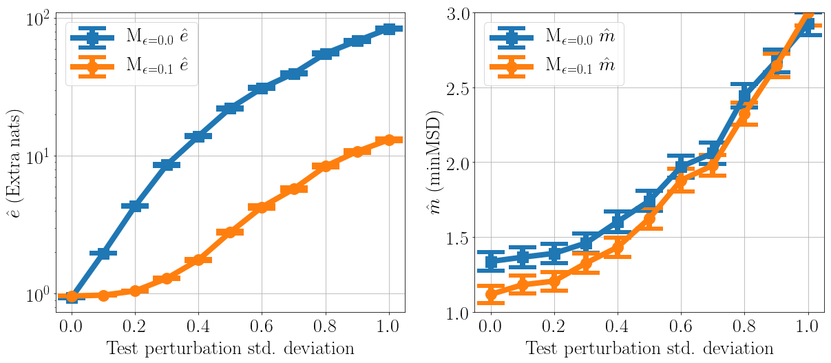
Refer to caption
Figure 11: Evaluating the effects of noisy localization on nuScenes A=2𝐴2A=2.
Refer to caption
Figure 12: Histogram of m^K=12subscript^𝑚𝐾12\hat{m}_{K=12} of forecasts made by the ESP flexible-count model on CARLA Town02 Test A=5𝐴5A=5, T=20𝑇20T=20 at 101010Hz (2 seconds of future). The median m^K=12subscript^𝑚𝐾12\hat{m}_{K=12} is 0.090.090.09.
Refer to caption
Figure 13: Histogram of m^K=12subscript^𝑚𝐾12\hat{m}_{K=12} of forecasts made by the ESP flexible-count model on nuScenes Test A=5𝐴5A=5, T=20𝑇20T=20 at 555Hz (4 seconds of future). The median m^K=12subscript^𝑚𝐾12\hat{m}_{K=12} is 1.311.311.31.
Refer to caption
(a) Plot of m^Ksubscript^𝑚𝐾\hat{m}_{K} vs. K𝐾K of the ESP flexible-count model on CARLA Town02 Test A=5𝐴5A=5, T=20𝑇20T=20 at 101010Hz (2s).
Refer to caption
(b) Plot of m^Ksubscript^𝑚𝐾\hat{m}_{K} vs. K𝐾K of the ESP flexible-count model on nuScenes Test A=5𝐴5A=5, T=20𝑇20T=20 at 555Hz (4s).
Figure 14: Mean m^Ksubscript^𝑚𝐾\hat{m}_{K} and its standard error vs. K𝐾K in two settings.
Figure 15: Forecasting evaluation of our model on CARLA Town01 Test and nuScenes Test data. Planning the robot to a goal position (PRECOG) generates better predictions for all agents. Means and their standard errors are reported. The en-dash (–) represents statistics of agents that are not present in a dataset.
Data Approach Test m^K=12subscript^𝑚𝐾12\hat{m}_{K=12} Test m^K=12a=1superscriptsubscript^𝑚𝐾12𝑎1\hat{m}_{K=12}^{a=1} Test m^K=12a=2superscriptsubscript^𝑚𝐾12𝑎2\hat{m}_{K=12}^{a=2} Test m^K=12a=3superscriptsubscript^𝑚𝐾12𝑎3\hat{m}_{K=12}^{a=3} Test m^K=12a=4superscriptsubscript^𝑚𝐾12𝑎4\hat{m}_{K=12}^{a=4} Test m^K=12a=5superscriptsubscript^𝑚𝐾12𝑎5\hat{m}_{K=12}^{a=5}
CARLA  A=2𝐴2A\!=\!2 DESIRE 1.83703±0.04810plus-or-minus1.837030.04810$1.83703$\pm$0.04810$ 1.99149±0.06605plus-or-minus1.991490.06605$1.99149$\pm$0.06605$ 1.68257±0.05013plus-or-minus1.682570.05013$1.68257$\pm$0.05013$
DESIRE-plan 1.85810±0.04614plus-or-minus1.858100.04614$1.85810$\pm$0.04614$ 0.91834±0.04441plus-or-minus0.918340.04441$0.91834$\pm$0.04441$ 2.79785±0.07331plus-or-minus2.797850.07331$2.79785$\pm$0.07331$
ESP 0.33705±0.0132plus-or-minus0.337050.0132$0.33705$\pm$0.0132$ 0.196±0.009plus-or-minus0.1960.009$0.196$\pm$0.009$ 0.478±0.024plus-or-minus0.4780.024$0.478$\pm$0.024$
PRECOG 0.2406397±0.01207plus-or-minus0.24063970.01207{\boldmath$0.2406397$\pm$0.01207$} 0.055±0.003plus-or-minus0.0550.003{\boldmath$0.055$\pm$0.003$} 0.426±0.024plus-or-minus0.4260.024{\boldmath$0.426$\pm$0.024$}
CARLA  A=3𝐴3A\!=\!3 DESIRE 1.69854±0.03154plus-or-minus1.698540.03154$1.69854$\pm$0.03154$ 1.56990±0.03743plus-or-minus1.569900.03743$1.56990$\pm$0.03743$ 1.66092±0.04731plus-or-minus1.660920.04731$1.66092$\pm$0.04731$ 1.86479±0.04663plus-or-minus1.864790.04663$1.86479$\pm$0.04663$
DESIRE-plan 2.34311±0.04724plus-or-minus2.343110.04724$2.34311$\pm$0.04724$ 0.23222±0.00896plus-or-minus0.232220.00896$0.23222$\pm$0.00896$ 3.12998±0.07784plus-or-minus3.129980.07784$3.12998$\pm$0.07784$ 3.66712±0.09646plus-or-minus3.667120.09646$3.66712$\pm$0.09646$
ESP 0.42641±0.01320plus-or-minus0.426410.01320$0.42641$\pm$0.01320$ 0.20427±0.00856plus-or-minus0.204270.00856$0.20427$\pm$0.00856$ 0.55607±0.02707plus-or-minus0.556070.02707$0.55607$\pm$0.02707$ 0.51887±0.02124plus-or-minus0.518870.02124$0.51887$\pm$0.02124$
PRECOG 0.35464±0.01170plus-or-minus0.354640.01170{\boldmath$0.35464$\pm$0.01170$} 0.05175±0.00339plus-or-minus0.051750.00339{\boldmath$0.05175$\pm$0.00339$} 0.51927±0.02536plus-or-minus0.519270.02536{\boldmath$0.51927$\pm$0.02536$} 0.49290±0.02036plus-or-minus0.492900.02036{\boldmath$0.49290$\pm$0.02036$}
CARLA  A=4𝐴4A\!=\!4 DESIRE 2.40163±0.03761plus-or-minus2.401630.03761$2.40163$\pm$0.03761$ 2.42204±0.05373plus-or-minus2.422040.05373$2.42204$\pm$0.05373$ 2.06456±0.04388plus-or-minus2.064560.04388$2.06456$\pm$0.04388$ 2.53084±0.07142plus-or-minus2.530840.07142$2.53084$\pm$0.07142$ 2.58909±0.06445plus-or-minus2.589090.06445$2.58909$\pm$0.06445$
DESIRE-plan 1.82801±0.03488plus-or-minus1.828010.03488$1.82801$\pm$0.03488$ 0.14943±0.00366plus-or-minus0.149430.00366$0.14943$\pm$0.00366$ 2.48027±0.06241plus-or-minus2.480270.06241$2.48027$\pm$0.06241$ 1.25603±0.04731plus-or-minus1.256030.04731$1.25603$\pm$0.04731$ 3.42629±0.09763plus-or-minus3.426290.09763$3.42629$\pm$0.09763$
ESP 0.53743±0.01120plus-or-minus0.537430.01120$0.53743$\pm$0.01120$ 0.23587±0.00893plus-or-minus0.235870.00893$0.23587$\pm$0.00893$ 0.61460±0.02142plus-or-minus0.614600.02142$0.61460$\pm$0.02142$ 0.65640±0.02283plus-or-minus0.656400.02283$0.65640$\pm$0.02283$ 0.64285±0.02342plus-or-minus0.642850.02342$0.64285$\pm$0.02342$
PRECOG 0.47798±0.01078plus-or-minus0.477980.01078{\boldmath$0.47798$\pm$0.01078$} 0.05397±0.00323plus-or-minus0.053970.00323{\boldmath$0.05397$\pm$0.00323$} 0.58304±0.02056plus-or-minus0.583040.02056{\boldmath$0.58304$\pm$0.02056$} 0.63710±0.02208plus-or-minus0.637100.02208{\boldmath$0.63710$\pm$0.02208$} 0.63779±0.02291plus-or-minus0.637790.02291{\boldmath$0.63779$\pm$0.02291$}
CARLA  A=5𝐴5A\!=\!5 DESIRE 2.62247±0.02953plus-or-minus2.622470.02953$2.62247$\pm$0.02953$ 2.62066±0.04547plus-or-minus2.620660.04547$2.62066$\pm$0.04547$ 2.42165±0.04842plus-or-minus2.421650.04842$2.42165$\pm$0.04842$ 2.71018±0.06613plus-or-minus2.710180.06613$2.71018$\pm$0.06613$ 2.96901±0.05700plus-or-minus2.969010.05700$2.96901$\pm$0.05700$ 2.39086±0.04891plus-or-minus2.390860.04891$2.39086$\pm$0.04891$
DESIRE-plan 2.32850±0.03837plus-or-minus2.328500.03837$2.32850$\pm$0.03837$ 0.19446±0.00359plus-or-minus0.194460.00359$0.19446$\pm$0.00359$ 2.23880±0.05707plus-or-minus2.238800.05707$2.23880$\pm$0.05707$ 3.11885±0.09775plus-or-minus3.118850.09775$3.11885$\pm$0.09775$ 3.33222±0.09021plus-or-minus3.332220.09021$3.33222$\pm$0.09021$ 2.75818±0.08278plus-or-minus2.758180.08278$2.75818$\pm$0.08278$
ESP 0.71759±0.01187plus-or-minus0.717590.01187$0.71759$\pm$0.01187$ 0.34031±0.01146plus-or-minus0.340310.01146$0.34031$\pm$0.01146$ 0.75908±0.02449plus-or-minus0.759080.02449$0.75908$\pm$0.02449$ 0.80909±0.02504plus-or-minus0.809090.02504$0.80909$\pm$0.02504$ 0.85122±0.02335plus-or-minus0.851220.02335$0.85122$\pm$0.02335$ 0.82827±0.02411plus-or-minus0.828270.02411$0.82827$\pm$0.02411$
PRECOG 0.64039±0.01109plus-or-minus0.640390.01109{\boldmath$0.64039$\pm$0.01109$} 0.06557±0.00348plus-or-minus0.065570.00348{\boldmath$0.06557$\pm$0.00348$} 0.74088±0.02363plus-or-minus0.740880.02363{\boldmath$0.74088$\pm$0.02363$} 0.79019±0.02449plus-or-minus0.790190.02449{\boldmath$0.79019$\pm$0.02449$} 0.80444±0.02238plus-or-minus0.804440.02238{\boldmath$0.80444$\pm$0.02238$} 0.80085±0.02401plus-or-minus0.800850.02401{\boldmath$0.80085$\pm$0.02401$}
nuScenes  A=2𝐴2A\!=\!2 DESIRE 3.30741±0.09280plus-or-minus3.307410.09280$3.30741$\pm$0.09280$ 3.00155±0.08819plus-or-minus3.001550.08819$3.00155$\pm$0.08819$ 3.61328±0.13969plus-or-minus3.613280.13969$3.61328$\pm$0.13969$
DESIRE-plan 4.52804±0.15055plus-or-minus4.528040.15055$4.52804$\pm$0.15055$ 0.45641±0.01544plus-or-minus0.456410.01544$0.45641$\pm$0.01544$ 8.59966±0.29765plus-or-minus8.599660.29765$8.59966$\pm$0.29765$
ESP 1.09373±0.05281plus-or-minus1.093730.05281$1.09373$\pm$0.05281$ 0.95464±0.05651plus-or-minus0.954640.05651$0.95464$\pm$0.05651$ 1.23282±0.07814plus-or-minus1.232820.07814$1.23282$\pm$0.07814$
PRECOG 0.51431±0.03667plus-or-minus0.514310.03667\boldmath$0.51431$\pm$0.03667$ 0.15778±0.01621plus-or-minus0.157780.01621\boldmath$0.15778$\pm$0.01621$ 0.87085±0.07002plus-or-minus0.870850.07002\boldmath$0.87085$\pm$0.07002$
nuScenes  A=3𝐴3A\!=\!3 DESIRE 4.84047±0.13493plus-or-minus4.840470.13493$4.84047$\pm$0.13493$ 3.93144±0.12722plus-or-minus3.931440.12722$3.93144$\pm$0.12722$ 4.98354±0.20695plus-or-minus4.983540.20695$4.98354$\pm$0.20695$ 5.60645±0.23404plus-or-minus5.606450.23404$5.60645$\pm$0.23404$
DESIRE-plan 5.88704±0.18713plus-or-minus5.887040.18713$5.88704$\pm$0.18713$ 0.40910±0.01451plus-or-minus0.409100.01451$0.40910$\pm$0.01451$ 7.73086±0.33673plus-or-minus7.730860.33673$7.73086$\pm$0.33673$ 9.52117±0.39943plus-or-minus9.521170.39943$9.52117$\pm$0.39943$
ESP 1.51103±0.07741plus-or-minus1.511030.07741$1.51103$\pm$0.07741$ 1.12817±0.06052plus-or-minus1.128170.06052$1.12817$\pm$0.06052$ 1.54337±0.11801plus-or-minus1.543370.11801$1.54337$\pm$0.11801$ 1.86155±0.14696plus-or-minus1.861550.14696$1.86155$\pm$0.14696$
PRECOG 1.01569±0.06249plus-or-minus1.015690.06249\boldmath$1.01569$\pm$0.06249$ 0.12111±0.00457plus-or-minus0.121110.00457\boldmath$0.12111$\pm$0.00457$ 1.32020±0.10501plus-or-minus1.320200.10501\boldmath$1.32020$\pm$0.10501$ 1.60576±0.12173plus-or-minus1.605760.12173\boldmath$1.60576$\pm$0.12173$
nuScenes  A=4𝐴4A\!=\!4 DESIRE 5.77079±0.15115plus-or-minus5.770790.15115$5.77079$\pm$0.15115$ 4.19479±0.15876plus-or-minus4.194790.15876$4.19479$\pm$0.15876$ 5.85411±0.24286plus-or-minus5.854110.24286$5.85411$\pm$0.24286$ 6.13803±0.28031plus-or-minus6.138030.28031$6.13803$\pm$0.28031$ 6.89623±0.32431plus-or-minus6.896230.32431$6.89623$\pm$0.32431$
DESIRE-plan 5.04545±0.15842plus-or-minus5.045450.15842$5.04545$\pm$0.15842$ 0.47126±0.01900plus-or-minus0.471260.01900$0.47126$\pm$0.01900$ 5.56701±0.24471plus-or-minus5.567010.24471$5.56701$\pm$0.24471$ 5.49193±0.25697plus-or-minus5.491930.25697$5.49193$\pm$0.25697$ 8.65161±0.40677plus-or-minus8.651610.40677$8.65161$\pm$0.40677$
ESP 2.20022±0.08957plus-or-minus2.200220.08957$2.20022$\pm$0.08957$ 1.60400±0.09882plus-or-minus1.604000.09882$1.60400$\pm$0.09882$ 1.94018±0.12261plus-or-minus1.940180.12261$1.94018$\pm$0.12261$ 2.40535±0.14867plus-or-minus2.405350.14867$2.40535$\pm$0.14867$ 2.85133±0.21334plus-or-minus2.851330.21334$2.85133$\pm$0.21334$
PRECOG 1.75499±0.08254plus-or-minus1.754990.08254\boldmath$1.75499$\pm$0.08254$ 0.13314±0.00591plus-or-minus0.133140.00591\boldmath$0.13314$\pm$0.00591$ 1.80359±0.12562plus-or-minus1.803590.12562\boldmath$1.80359$\pm$0.12562$ 2.31905±0.14119plus-or-minus2.319050.14119\boldmath$2.31905$\pm$0.14119$ 2.76419±0.23126plus-or-minus2.764190.23126\boldmath$2.76419$\pm$0.23126$
nuScenes  A=5𝐴5A\!=\!5 DESIRE 6.82986±0.20435plus-or-minus6.829860.20435$6.82986$\pm$0.20435$ 4.99886±0.21870plus-or-minus4.998860.21870$4.99886$\pm$0.21870$ 6.41475±0.29442plus-or-minus6.414750.29442$6.41475$\pm$0.29442$ 7.02696±0.36014plus-or-minus7.026960.36014$7.02696$\pm$0.36014$ 7.41826±0.32365plus-or-minus7.418260.32365$7.41826$\pm$0.32365$ 8.29048±0.53172plus-or-minus8.290480.53172$8.29048$\pm$0.53172$
DESIRE-plan 6.56219±0.20719plus-or-minus6.562190.20719$6.56219$\pm$0.20719$ 2.26053±0.09984plus-or-minus2.260530.09984$2.26053$\pm$0.09984$ 6.64410±0.31435plus-or-minus6.644100.31435$6.64410$\pm$0.31435$ 6.18376±0.32513plus-or-minus6.183760.32513$6.18376$\pm$0.32513$ 9.20305±0.44800plus-or-minus9.203050.44800$9.20305$\pm$0.44800$ 8.51950±0.51390plus-or-minus8.519500.51390$8.51950$\pm$0.51390$
ESP 2.92126±0.17499plus-or-minus2.921260.17499$2.92126$\pm$0.17499$ 1.86066±0.10935plus-or-minus1.860660.10935$1.86066$\pm$0.10935$ 2.36853±0.18780plus-or-minus2.368530.18780$2.36853$\pm$0.18780$ 2.81241±0.18794plus-or-minus2.812410.18794$2.81241$\pm$0.18794$ 3.20137±0.25363plus-or-minus3.201370.25363$3.20137$\pm$0.25363$ 4.36335±0.65235plus-or-minus4.363350.65235$4.36335$\pm$0.65235$
PRECOG 2.50763±0.15214plus-or-minus2.507630.15214\boldmath$2.50763$\pm$0.15214$ 0.14913±0.02075plus-or-minus0.149130.02075\boldmath$0.14913$\pm$0.02075$ 2.32361±0.18743plus-or-minus2.323610.18743\boldmath$2.32361$\pm$0.18743$ 2.65441±0.19017plus-or-minus2.654410.19017\boldmath$2.65441$\pm$0.19017$ 3.15719±0.27262plus-or-minus3.157190.27262\boldmath$3.15719$\pm$0.27262$ 4.25379±0.58602plus-or-minus4.253790.58602\boldmath$4.25379$\pm$0.58602$

F.2 Additional CARLA and nuScenes Evaluations.

We show additional evaluations on CARLA in Tab. 3. Table 3 shows the Town01 of the models trained on Town01 (on separate episodes). We show single-agent CARLA forecasting results in Tab. 4. We show histograms of m^^𝑚\hat{m} in Fig. 12, Fig. 13, and Fig. 16. We show a comparison to longer time-horizon forecasting in Tab. 5. We show a plot of means and their standard errors of m^Ksubscript^𝑚𝐾\hat{m}_{K} vs. K𝐾K in Fig. 14.

Table 5: Performance on CARLA Town01 Test with T=40𝑇40T=40 at 101010Hz (4 seconds of future). This data has larger dimensionality than CARLA T=20𝑇20T=20, 101010Hz (2 seconds) data and the nuScenes T=20𝑇20T=20, 555Hz (4 seconds) data.
Approach Test m^K=12subscript^𝑚𝐾12\hat{m}_{K\!=\!12} Test e^^𝑒\hat{e}
(minMSD) (extra nats)
Town01 Test, T=20𝑇20T=20, 101010Hz (2s) 5 agent
ESP, flex. count 0.446775±0.009190plus-or-minus0.4467750.009190$0.446775$\pm$0.009190$ 0.508599±0.001097plus-or-minus0.5085990.001097$0.508599$\pm$0.001097$
Town02 Test, T=20𝑇20T=20, 101010Hz (2s) 5 agent
ESP, flex. count 0.435110±0.010517plus-or-minus0.4351100.010517$0.435110$\pm$0.010517$ 0.495612±0.001090plus-or-minus0.4956120.001090$0.495612$\pm$0.001090$
Town01 Test, T=40𝑇40T=40, 101010Hz (4s) 5 agent
ESP, flex. count 2.500401±0.076503plus-or-minus2.5004010.076503$2.500401$\pm$0.076503$ 0.491603±0.001252plus-or-minus0.4916030.001252$0.491603$\pm$0.001252$
nuScenes Test, T=20𝑇20T=20, 555Hz (4s) 5 agent
ESP, flex. count 2.933192±0.128841plus-or-minus2.9331920.128841$2.933192$\pm$0.128841$ 1.028862±0.002387plus-or-minus1.0288620.002387$1.028862$\pm$0.002387$

F.3 Full Conditional Forecasting Experiments

Due to main-text space limits, we report some remaining results (i.e. for A={3,4}𝐴34A=\{3,4\}) in Tab. 15. We observe similar trends in these results as in A=2𝐴2A=2 and A=5𝐴5A=5: PRECOG improves predictions of all agents’ future trajectories, and that knowledge of the ego-agent’s goal provides improves predictions for closer agents more than farther agents.

Appendix G Additional Visualizations

We display additional visualization of our results in Figures 18, 19, 20, 21, and 24. In Fig. 18, we show additional forecasting results on the nuScenes dataset. In Fig. 19, we show additional forecasting results on the CARLA dataset. In Fig. 20, we show additional planning results on the CARLA dataset. In Fig. 21, we show additional planning results on the nuScenes dataset. In Fig. 22, we show qualitative results of high, medium, and low quality on the CARLA A=5𝐴5A=5 dataset (ordered by m^^𝑚\hat{m}), paired with their corresponding m^^𝑚\hat{m} scores. In Fig. 23, we show qualitative results of high, medium, and low quality on the nuScenes A=5𝐴5A=5 dataset (ordered by m^^𝑚\hat{m}), paired with their corresponding m^^𝑚\hat{m} scores. In Fig. 24, we visualize the planning criterion (L^^𝐿\hat{L}) across many different spatio-temporal goal positions in CARLA, which gives a qualitative interpretation of where the model prefers goal. In Fig. 25, we visualize the same posterior on nuScenes.
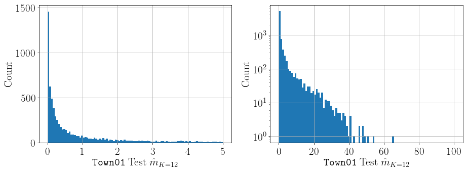
Refer to caption
Figure 16: Histogram of m^K=12subscript^𝑚𝐾12\hat{m}_{K=12} of forecasts made by the ESP flexible-count model on CARLA Town01 Test A=5𝐴5A=5, T=40𝑇40T=40 at 101010Hz (4 seconds of future). The median m^K=12subscript^𝑚𝐾12\hat{m}_{K=12} is 0.380.380.38.
Refer to caption
(a) Plot of m^Ksubscript^𝑚𝐾\hat{m}_{K} vs. K𝐾K of the ESP flexible-count model on CARLA Town01 Test A=5𝐴5A=5, T=40𝑇40T=40 at 101010Hz (4s).

Figure 18: Example forecasting results on held-out nuScenes data with our learned ESP model. In each scene, 12 joint samples are shown, and LIDAR colors are discretized to near-ground and above-ground

Refer to caption
Refer to caption
Refer to caption
Refer to caption
Refer to caption
Refer to caption
Refer to caption
Refer to caption
Refer to caption
Refer to caption
Refer to caption
Refer to caption
Figure 19: Examples of multi-agent forecasting with our learned ESP model. In each scene, 12 joint samples are shown, and LIDAR colors are discretized to near-ground and above-ground.
Refer to caption
(a) Scene 1, forecasted
Refer to caption
(b) Scene 1, planned
Refer to caption
(c) Scene 2, forecasted
Refer to caption
(d) Scene 2, planned
Refer to caption
(e) Scene 3, forecasted
Refer to caption
(f) Scene 3, planned
Refer to caption
(g) Scene 4, forecasted
Refer to caption
(h) Scene 4, planned
Figure 20: Additional examples of planned multi-agent forecasting (PRECOG) with our learned model in CARLA. By using our planning approach and conditioning the robot on its true final position, our predictions for the robot become more accurate, and often our predictions of the other agent become more accurate.
Refer to caption
(a) Scene 1, forecasted
Refer to caption
(b) Scene 1, planned
Refer to caption
(c) Scene 2, forecasted
Refer to caption
(d) Scene 2, planned
Refer to caption
(e) Scene 3, forecasted
Refer to caption
(f) Scene 3, planned
Figure 21: Additional examples of planned multi-agent forecasting (PRECOG) with our learned model in nuScenes. By using our planning approach and conditioning the robot on its true final position, our predictions for the robot become more accurate, and often our predictions of the other agent become more accurate.
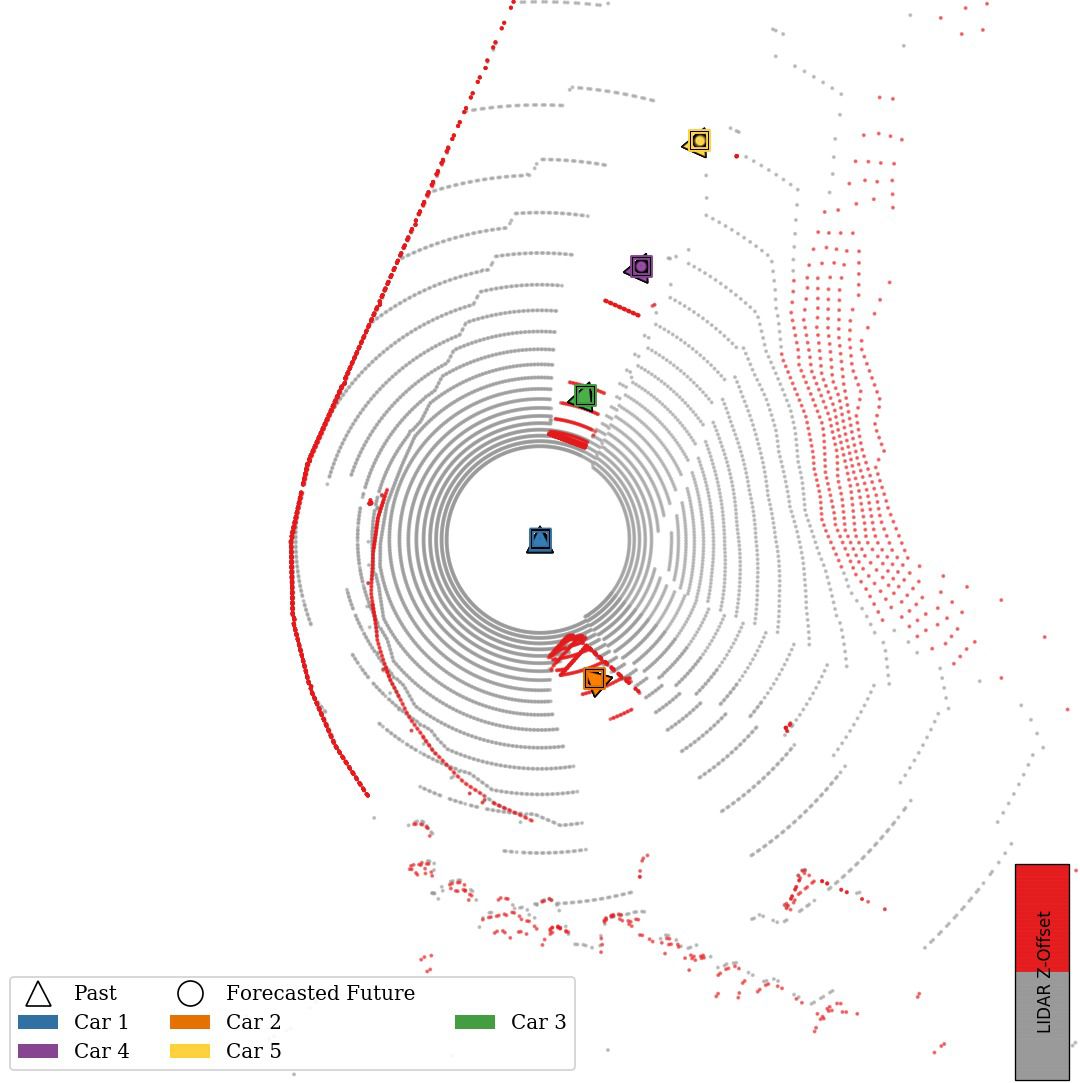
Refer to caption
(a) Best (>99%absentpercent99>99\%). m^K=12=0.00038554936subscript^𝑚𝐾120.00038554936\hat{m}_{K=12}=$0.00038554936$
Refer to caption
(b) Best (>99%absentpercent99>99\%). m^K=12=0.00040327205subscript^𝑚𝐾120.00040327205\hat{m}_{K=12}=$0.00040327205$
Refer to caption
(c) Best (>99%absentpercent99>99\%). m^K=12=0.00054206065subscript^𝑚𝐾120.00054206065\hat{m}_{K=12}=$0.00054206065$

Refer to caption
(d) Median (50%absentpercent50\approx 50\%). m^K=12=0.3816643subscript^𝑚𝐾120.3816643\hat{m}_{K=12}=$0.3816643$
Refer to caption
(e) Median (50%absentpercent50\approx 50\%). m^K=12=0.37981653subscript^𝑚𝐾120.37981653\hat{m}_{K=12}=$0.37981653$
Refer to caption
(f) Median (50%absentpercent50\approx 50\%). m^K=12=0.3687198subscript^𝑚𝐾120.3687198\hat{m}_{K=12}=$0.3687198$
Refer to caption
(g) Worst (<0.2%absentpercent0.2\!<\!0.2\%). m^K=12=64.738914subscript^𝑚𝐾1264.738914\hat{m}_{K=12}\!=\!$64.738914$
Refer to caption
(h) Worst (<0.2%absentpercent0.2<0.2\%). m^K=12=41.256767subscript^𝑚𝐾1241.256767\hat{m}_{K=12}=$41.256767$
Refer to caption
(i) Worst (<0.2%absentpercent0.2<0.2\%). m^K=12=41.18337subscript^𝑚𝐾1241.18337\hat{m}_{K=12}=$41.18337$
Figure 22: Various qualities (Row 1: 100%absentpercent100\approx 100\%, Row 2: 50%absentpercent50\approx 50\%, and Row 3: 0%absentpercent0\approx 0\%) of qualitative results of the ESP flex. count model on Town01 Test, A=5𝐴5A=5, T=40𝑇40T=40 at 101010Hz (4 seconds of future), ordered by m^K=12subscript^𝑚𝐾12\hat{m}_{K=12}. Recall since m^^𝑚\hat{m} is a joint-agent statistic, per-agent trajectory sample coverage is insufficient for a good m^^𝑚\hat{m} score. Also, recall m^^𝑚\hat{m} measures the error of the closest joint trajectory to the true future, as opposed to the error of all joint trajectories, which is key to its property of not penalizing otherwise-plausible trajectories.

Refer to caption
(a) Best (99%absentpercent99\approx 99\%). m^K=12=0.00031447396subscript^𝑚𝐾120.00031447396\hat{m}_{K=12}\!=\!$0.00031447396$
Refer to caption
(b) Best (94%absentpercent94\approx 94\%). m^K=12=0.023256572subscript^𝑚𝐾120.023256572\hat{m}_{K=12}\!=\!$0.023256572$
Refer to caption
(c) Best (93%absentpercent93\approx 93\%). m^K=12=0.028836906subscript^𝑚𝐾120.028836906\hat{m}_{K=12}\!=\!$0.028836906$
Refer to caption
(d) Median (50%absentpercent50\approx 50\%). m^K=12=1.3064103subscript^𝑚𝐾121.3064103\hat{m}_{K=12}\!=\!$1.3064103$
Refer to caption
(e) Median (50%absentpercent50\approx 50\%). m^K=12=1.3085703subscript^𝑚𝐾121.3085703\hat{m}_{K=12}\!=\!$1.3085703$
Refer to caption
(f) Median (50%absentpercent50\approx 50\%). m^K=12=1.3270347subscript^𝑚𝐾121.3270347\hat{m}_{K=12}\!=\!$1.3270347$
Refer to caption
(g) Worst (<3%absentpercent3\!<\!3\%). m^K=12=15.592783subscript^𝑚𝐾1215.592783\hat{m}_{K=12}\!=\!$15.592783$
Refer to caption
(h) Worst (<3%absentpercent3\!<\!3\%). m^K=12=13.391655subscript^𝑚𝐾1213.391655\hat{m}_{K=12}\!=\!$13.391655$
Refer to caption
(i) Worst (<3%absentpercent3\!<\!3\%). m^K=12=11.520764subscript^𝑚𝐾1211.520764\hat{m}_{K=12}\!=\!$11.520764$
Figure 23: Various qualities (Row 1: 100%absentpercent100\approx 100\%, Row 2: 50%absentpercent50\approx 50\%, and Row 3: 0%absentpercent0\approx 0\%) of qualitative results of the ESP flex. count model on nuScenes Test, A=5𝐴5A=5, T=20𝑇20T=20 at 555Hz (4 seconds of future), ordered by m^K=12subscript^𝑚𝐾12\hat{m}_{K=12}. Recall since m^^𝑚\hat{m} is a joint-agent statistic, per-agent trajectory sample coverage is insufficient for a good m^^𝑚\hat{m} score. Also, recall m^^𝑚\hat{m} measures the error of the closest joint trajectory to the true future, as opposed to the error of all joint trajectories, which is key to its property of not penalizing otherwise-plausible trajectories.

Refer to caption
Refer to caption
Refer to caption

Refer to caption
Refer to caption
Refer to caption

Refer to caption
Refer to caption
Refer to caption

Refer to caption
Refer to caption
Refer to caption
Refer to caption
Figure 24: Plotting the planning criterion, L^^𝐿\hat{L}, after planning to various positions (small circular dots in each plot) input to Alg. 3, with values interpolated between each position, in CARLA. The planning criterion input corresponds to a spatio-temporal goal at T=20𝑇20T=20 in the future (444 seconds). The planning criterion prefers locations within its lane, unless it is uncertain about the possibility of turning. When the vehicle was stationary in the past, the planning criterion is highest at positions at or close in front of the vehicle.

Refer to caption
Refer to caption
Refer to caption
Refer to caption
Refer to caption
Refer to caption

Refer to caption
Refer to caption
Refer to caption

Refer to caption
Refer to caption
Refer to caption
Refer to caption
Figure 25: Plotting the planning criterion, L^^𝐿\hat{L}, after planning to various positions (small circular dots in each plot) input to Alg. 3, with values interpolated between each position, in nuScenes. The planning criterion input corresponds to a spatio-temporal goal at T=20𝑇20T=20 in the future (444 seconds). The planning criterion prefers locations within its lane, unless it is uncertain about the possibility of turning. When the vehicle was stationary in the past, the planning criterion is highest at positions at or close in front of the vehicle.