Zihang Laizihang.lai@cs.ox.ac.uk1
\addauthorWeidi Xieweidi@robots.ox.ac.uk2
\addinstitution
Department of Computer Science
University of Oxford, UK
\addinstitution
Visual Geometry Group,
Department of Engineering Science
University of Oxford, UK
Self-supervised Learning for Video Correspondence Flow
\useunder\ul
\newfloatcommandcapbtabboxtable[][\FBwidth]
Self-supervised Learning for Video Correspondence Flow
Abstract
The objective of this paper is self-supervised learning of feature embeddings that are suitable for matching correspondences along the videos, which we term correspondence flow. By leveraging the natural spatial-temporal coherence in videos, we propose to train a “pointer” that reconstructs a target frame by copying pixels from a reference frame.
We make the following contributions: First, we introduce a simple information bottleneck that forces the model to learn robust features for correspondence matching, and prevent it from learning trivial solutions, e.g\bmvaOneDotmatching based on low-level colour information. Second, to alleveate tracker drifting, due to complex object deformations, illumination changes and occlusions, we propose to train a recursive model over long temporal windows with scheduled sampling and cycle consistency. Third, we achieve the state-of-the-art performance on DAVIS 2017 video segmentation and JHMDB keypoint tracking tasks, outperforming all previous self-supervised learning approaches by a significant margin. Fourth, in order to shed light on the potential of self-supervised learning on the task of video correspondence flow, we probe the upper bound by training on additional data, i.e\bmvaOneDotmore diverse videos, further demonstrating significant improvements on video segmentation. The source code will be released at https://github.com/zlai0/CorrFlow.
1 Introduction
Correspondence matching is a fundamental building block for numerous applications ranging from depth estimation [Kendall et al.(2017)Kendall, Martirosyan, Dasgupta, Henry, Kennedy, Bachrach, and Bry] and optical flow [Brox et al.(2004)Brox, Bruhn, Papenberg, and Weickert, Dosovitskiy et al.(2015)Dosovitskiy, Fischer, Ilg, Hausser, Hazirbas, Golkov, Smagt, Cremers, and Brox, Ilg et al.(2017)Ilg, Mayer, Saikia, Keuper, Dosovitskiy, and Brox], to segmentation and tracking [Smith and Brady(1995)], and 3D reconstruction [Hartley and Zisserman(2004)]. However, training models for correspondence matching is not trivial, as obtaining manual annotations can be prohibitively expensive, and sometimes is even impossible due to occlusions and complex object deformations. In the recent works [Rocco et al.(2017)Rocco, Arandjelovic, and Sivic, Rocco et al.(2018)Rocco, Arandjelovic, and Sivic], Rocco et al\bmvaOneDotproposed to circumvent this issue by pre-training Convolutional Neural Networks (CNNs) for predicting artificial transformations, and further bootstrap the model by finetuning on a small dataset with human annotations. Alternatively, the necessity for labbelled data can be avoided by using self-supervised learning, i.e\bmvaOneDota form of unsupervised learning, where part of the data is withheld for defining a proxy task, such that the model will be forced to learn the semantic representation that we really care about.
Videos have shown to be appealing as a data source for self-supervised learning due to their almost infinite supply (from YouTube etc), and the availability of numerous proxy losses that can be employed from the intrinsic spatio-temporal coherence, i.e\bmvaOneDotthe signals in video tend to vary smoothly in time [Wiskott and Sejnowski(2002), Jayaraman and Grauman(2016)]. In this paper, we propose to tackle the task of correspondence flow in videos with self-supervised learning. We are certainly not the first to explore this idea, in the seminal paper by Vondrick et al\bmvaOneDot [Vondrick et al.(2018)Vondrick, Shrivastava, Fathi, Guadarrama, and Murphy], they propose to learn embeddings for grayscale frames and use colorization as a proxy task for training. Despite the promising efforts, the model capacity has been significantly constrained due to the loss of colour information, and suffers the problem of tracker drifting as only pair of frames are used during training.
 |
 |
| (a) DAVIS 2017 Video Segmentation | (b) Keypoint Tracking |
We make the following contributions: First, we introduce an embarrassingly simple idea to avoid trivial solutions while learning pixelwise matching by frame reconstruction. During training, channel-wise dropout and colour jitterings are added intentionally on the input frames, the model is therefore forced not to rely on low-level colour information, and must be robust to colour jittering. Second, we propose to train the model recursively on videos over long temporal windows with scheduled sampling and forward-backward consistency. Both ideas have shown to improve the model robustness and help to alleviate the tracker drifting problem. Third, after self-supervised training, we benchmark the model on two downstream tasks focusing on pixelwise tracking, e.g\bmvaOneDotDAVIS 2017 video segmentation and JHMDB keypoint tracking, outperforming all previous self-supervised learning approaches by a significant margin. Fourth, to further shed light on the potential of self-supervised learning for video correspondence flow, we probe the upper bound by training on more diverse video data, and further demonstrating significant improvements on video segmentation.
2 Related Work
Correspondence Matching. Recently, many researchers have studied the task of correspondence matching using deep Convolutional Neural Networks [Han et al.(2017)Han, Rezende, Ham, Wong, Cho, Schmid, and Ponce, Kim et al.(2017)Kim, Min, Ham, Jeon, Lin, and Sohn, Novotny et al.(2017)Novotny, Larlus, and Vedaldi, Rocco et al.(2017)Rocco, Arandjelovic, and Sivic, Rocco et al.(2018)Rocco, Arandjelovic, and Sivic]. The works from Rocco et al\bmvaOneDot [Rocco et al.(2017)Rocco, Arandjelovic, and Sivic, Rocco et al.(2018)Rocco, Arandjelovic, and Sivic], propose to train CNNs by learning the artificial transformations between pairs of images. For robust estimation, they applied a differentiable soft inlier score for evaluating the quality of alignment between spatial features and providing a loss for learning semantic correspondences. However, their work may not be ideal as the model still relies on synthetic transformations. In contrast, we address the challenge of learning correspondence matching by exploiting the temporal coherence in videos.
Optical Flow. In the conventional variational approaches, optical flow estimation is treated as an energy minimization problem based on brightness constancy and spatial smoothness [Horn and Schunck(1981)]. In later works, feature matching is used to firstly establish sparse matchings, and then interpolated into dense flow maps in a pyramidal coarse-to-fine manner [Brox et al.(2009)Brox, Bregler, and Malik, Revaud et al.(2015)Revaud, Weinzaepfel, Harchaoui, and Schmid, Weinzaepfel et al.(2013)Weinzaepfel, Revaud, Harchaoui, and Schmid]. Recently, convolutional neural networks (CNNs) have been applied to improve the matching by learning effective feature embeddings [Bailer et al.(2017)Bailer, Varanasi, and Stricker, Jia et al.(2017)Jia, Ranftl, and Koltun]. Another line of more relevant research is unsupervised learning for optical flow. The basic principles are based on brightness constancy and spatial smoothness [Yu et al.(2016)Yu, Harley, and Derpanis, Wang et al.(2018)Wang, Yang, Yang, Zhao, Wang, and Xu, Meister et al.(2018)Meister, Hur, and Roth]. This leads to the popular photometric loss which measures the difference between the reference image and the warped image. For occluded regions, a mask is implicitly estimated by checking forward-backward consistency.
Self-supervised Learning. Of more direct relevance to our training framework are self-supervised frameworks that use video data [Agrawal et al.(2015)Agrawal, Carreira, and Malik, Denton and Birodkar(2017), Fernando et al.(2017)Fernando, Bilen, Gavves, and Gould, Gan et al.(2018)Gan, Gong, Liu, Su, and Guibas, Jakab et al.(2018)Jakab, Gupta, Bilen, and Vedaldi, Jia et al.(2016)Jia, De Brabandere, and Tuytelaars, Lee et al.(2017)Lee, Huang, Singh, and Yang, Misra et al.(2016)Misra, Zitnick, and Hebert, Wang and Gupta(2015), Wiles et al.(2018)Wiles, Koepke, and Zisserman, Isola et al.(2015)Isola, Zoran, Krishnan, and Adelson, Jayaraman and Grauman(2016), Jayaraman and Grauman(2015), Jing and Tian(2018), Kim et al.(2018)Kim, Cho, and Kweon, Vondrick et al.(2018)Vondrick, Shrivastava, Fathi, Guadarrama, and Murphy]. In [Misra et al.(2016)Misra, Zitnick, and Hebert, Fernando et al.(2017)Fernando, Bilen, Gavves, and Gould, Wei et al.(2018)Wei, Lim, Zisserman, and Freeman], the proxy task is defined to focus on temporal sequence ordering of the frames. Another approach is to use the temporal coherence as a proxy loss [Isola et al.(2015)Isola, Zoran, Krishnan, and Adelson, Jayaraman and Grauman(2016), Wang and Gupta(2015)]. Other approaches use egomotion [Agrawal et al.(2015)Agrawal, Carreira, and Malik, Jayaraman and Grauman(2015)] in order to enforce equivariance in feature space [Jayaraman and Grauman(2015)]. Recently [Vondrick et al.(2018)Vondrick, Shrivastava, Fathi, Guadarrama, and Murphy], leveraged the natural temporal coherency of colour in videos, to train a network for tracking and correspondence related tasks. Our approach builds in particular on those that use frame synthesis [Denton and Birodkar(2017), Jia et al.(2016)Jia, De Brabandere, and Tuytelaars, Wiles et al.(2018)Wiles, Koepke, and Zisserman], though for us synthesis is a proxy task rather than the end goal.
3 Approach
The goal of this work is to train an embedding network with self-supervised learning that enables pixelwise correspondence matching. Our basic idea is to exploit spatial-temporal coherence in videos, that is, the frame appearances will not change abruptly, and colours can act as a reliable supervision signal for learning correspondences.
3.1 Background
In this section, we briefly review the work by Vondrick et al\bmvaOneDot [Vondrick et al.(2018)Vondrick, Shrivastava, Fathi, Guadarrama, and Murphy]. Formally, let be the true colour for pixel in the reference frame, and let be the true colour for a pixel in the target frame. is the model’s prediction for , it is a linear combination of colours in the reference frame:
| (1) |
is an affinity matrix computed from simple dot products between the feature embeddings of the grayscale target and reference frame (’s).
Despite the efforts in circumventing trivial solutions, training models with grayscale inputs has introduces a train-test discrepancy when deploying to the downstream task, as the model has never been trained to encode the correlation of RGB channels. Another issule lies in the fact that their model is only trained with pairs of ground truth video frames, which inevitably leads to model drifting when evaluated on video tracking tasks. As the prediction for later steps rely on the prediction from previous steps, the errors accumulate, and there is no mechanism for the model to recover from previous error states.
In the following sections, we propose to train a framework that aims to close the gap between training and testing as much as possible, i.e\bmvaOneDotthe model should ideally be trained on full-colour and high-resolution over long video sequences.

3.2 Feature Embedding with Information Bottleneck
Given a collection of frames from a video clip, we parametrize the feature embedding module with CNNs:
| (2) |
where refers to a ResNet feature encoder (details in Arxiv paper111https://arxiv.org/abs/1905.00875), and denotes an information bottleneck that prevents from information leakage. In Vondrick et al\bmvaOneDot [Vondrick et al.(2018)Vondrick, Shrivastava, Fathi, Guadarrama, and Murphy], this is simply defined as a function that converts RGB frame into grayscale, therefore, the model is forced not to rely on colours for matching correspondences.
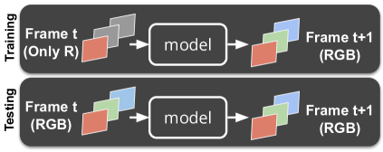
We propose to randomly zero out 0, 1, or 2 channels in each input frame with some probability (one possible input is shown in Figure 3 (a)), and perturb the brightness, contrast and saturation of an image by up to . Despite the simplicity, this design poses two benefits: First, the input jitterings and stochastic dropout are essentially acting as an information bottleneck, which prevents the model from co-adaptation of low-level colours. When deploying for downstream tasks, images of full RGB colours are taken as input directly (no jittering). Second, it can also be treated as data augmentation that potentially improves the model robustness under challenging cases, for instance, illumination changes.
3.3 Restricted Attention
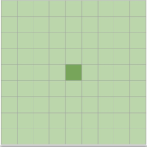
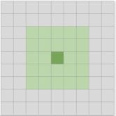
In the previous work [Vondrick et al.(2018)Vondrick, Shrivastava, Fathi, Guadarrama, and Murphy], full attention has been used for computing the affinity matrix, i.e\bmvaOneDotall pairs of pixels in target and reference frames are correlated (Figure 3 (b)). However, the memory and computational consumption tends to grow quadratically with the spatial footprint of the feature maps, thus limiting the resolution. In fact, videos are full of regularities, i.e\bmvaOneDotthe appearances in the video clip tend to change smoothly both in spatial and temporal axes. To fully exploit this property, we propose to use a restricted attention mechanism (Figure 3 (c)), which leads to dramatic decrease in computation and memory consumption, and enables to train on high-resolution frames.
 |
 |
 |
|||
| (a) Colour Dropout | (b) Full Attention | (c) Restricted Attention |
Specifically, we impose a maximum disparity of , i.e\bmvaOneDotpixels in the reference frame are searched for locally in a square patch of size , centered at the target pixel. Suppose the feature maps have a dimension of , the affinity volume () is therefore a tensor of dimension . The entry of the tensor denotes the similarity between pixel of the target frame, and pixel of the reference frame.
| (3) | ||||
| (4) |
where , and refer to the feature embeddings for frame and respectively. denotes a soft-copy operation for reconstructing by “borrowing” colours from frame.
3.4 Long-term Correspondence Flow
One of the challenges on self-supervised learning of correspondence flow is how to sample the training frames; If two frames are sampled closely in the temporal axis, the objects remain unchanged in both appearance and spatial position, matching becomes a trivial task and the model will not benefit from training on them. In the contrary, if the frames are sampled with a large temporal stride, the assumption of using reconstruction as supervision may fail, due to complex object deformation, illumination change, motion blurs, and occlusions.
In this section, we propose two approaches to improve the model’s robustness to tracker drifting, and gently bridge the gap of training with samples that are neither easy nor that difficult, i.e\bmvaOneDotscheduled sampling, and cycle consistency.
3.4.1 Scheduled Sampling
Scheduled sampling is a widely used curriculum learning strategy for sequence-to-sequence models [Bengio et al.(2015)Bengio, Vinyals, Jaitly, and Shazeer], the main idea is to replace some ground truth tokens by the model’s prediction, therefore improve the robustness and bridge the gap between train and inference stage.
In our case, for frames in a video sequence, a shared embedding network is used to get feature embeddings ( where ), the reconstruction is therefore formalized as a recursive process:
while reconstructing the th frame (), the model may have access to the previous frame as either groundtruth () or model prediction (). During training, the probability of using ground truth frames starts from a higher value () in early training stage, and is uniformly annealed to a probability of . Note that, as the model is recursive, the scheduled sampling forces the model to recover from error states and to be robust to drifting.
3.4.2 Cycle Consistency
Following the scheduled sampling, we also explicitly adopt a cycle consistency for training correspondence flow. Unlike [Wang et al.(2019b)Wang, Jabri, and Efros], we do not use the cycle consistency as the dominating supervision signal, instead, it is treated as another regularizer for combating drifting. During training, we apply our model frames forward and backward to the current frame.
3.5 Training Objectives
Similar to [Vondrick et al.(2018)Vondrick, Shrivastava, Fathi, Guadarrama, and Murphy], we pose frame reconstruction as a classification problem, the colour for each pixel is quantized into classes with K-means clustering in the Lab space. The objective function is defined as :
| (5) |
where refer to the pixel-wise cross entropy between groundtruth and reconstructed frames in the forward and backward paths, the loss weights for both paths are set as , respectively, i.e\bmvaOneDotforward path is weighted more than backward path.
4 Experiments and Analysis
In the following sections, we start with the training details, followed by ablation studies, e.g\bmvaOneDotcolour dropout, restricted attention, scheduled sampling and cycle consistency.
Training Details In this paper, we train CNNs in a completely self-supervised manner on Kinetics [Kay et al.(2017)Kay, Carreira, Simonyan, Zhang, Hillier, Vijayanarasimhan, F., Green, Natsev, Suleyman, and Zisserman], meaning we do not use any information other than video sequences, and not finetune for any target task. As pre-processing, we decode the videos with a frame rate of fps, and resize all frames to . In all of our experiments, we use a variant of ResNet-18 as a feature encoder (we refer the reader to our Arxiv paper for more details222https://arxiv.org/abs/1905.00875). which ends up with feature embeddings with spatial resolution of the original image. The max disparity in the restricted attention is set to be (as described in Section 3.3). The temporal length is set to in our case, so when considering the forward-backward cycles, the sequence length is actually frames. We train our model end-to-end using a batch size of for 1M iterations with an Adam optimizer. The initial learning rate is set to , and halved on 0.4, 0.6 and 0.8M iterations.
Evaluation Metrics In this paper, we report results on two public benchmarks: video segmentation, and pose keypoint propagation. For both tasks, a ground truth annotation is given for the first frame, and the objective is to propagate the mask to subsequent frames. In video segmentation, we benchmark our model on DAVIS-2017 [Pont-Tuset et al.(2017)Pont-Tuset, F., Caelles, Arbeláez, Sorkine-Hornung, and Van Gool], two standard metrics are used, i.e\bmvaOneDotregion overlapping () and contour accuracy (). For pose keypoint tracking, we evaluate our model on JHMDB dataset and report two different PCK metrics. The first (PCKinstance) considers a keypoint to be correct if the Normalized Euclidean Distance between that keypoint and the ground truth is smaller than a threshold . The second (PCKmax) accepts a keypoint if it is located within pixels of the ground truth, where and are the width and height of the instance bounding box.
4.1 Video Segmentation on DAVIS-2017
4.1.1 Ablation Studies
To examine the effects of different components, we conduct a series of ablation studies by removing one component at a time. All models are trained from scratch on Kinetics, and evaluated on the video segmentation task (DAVIS-2017) without finetuning.
| Method | (Mean) | (Mean) | |
|---|---|---|---|
| Ours (Full Model) | 47.7 | 51.3 | |
| Ours w/o Colour Dropout | 40.5 | 39.5 | |
| Ours w/o Restricted Attention | 40.8 | 39.7 | |
| Ours w/o Scheduled Sampling | 40.2 | 39.2 | |
| Ours w/o Cycle Consistency | 41.0 | 40.4 |
Colour Dropout Instead of taking full-colour input, we follow Vondrick et al\bmvaOneDot [Vondrick et al.(2018)Vondrick, Shrivastava, Fathi, Guadarrama, and Murphy], and convert all frames into grayscale for inputs. As shown in Table 5, both metrics drop significantly, i.e\bmvaOneDot in and in . This demonstrates the importance of bridging the discrepancy between training and testing on utilizing full-RGB colour information.
Restricted Attention When computing the affinity matrix with full attention, the model makes use of about G of GPU memory to process a single p image, it is therefore impossible to train on high-resolution frames with large batch size on standard GPUs (12-24GB). In comparison, our model with restricted attention only takes G GPU memory for the same image. As Table 5 shows, performance dropped by and on and before or after using restricted attention. This decrease confirms our assumption about spatial coherence in videos, leading both a decrease of memory consumption, and an effective regularizer that avoids the model matching correspondences very far away, for instance matching repeated patterns along the entire image.
Scheduled Sampling When not using the scheduled sampling, i.e\bmvaOneDotall frames used for copying are groundtruth during training, the performance dropped significantly from to in , to in , suggesting that the scheduled sampling indeed improves the model robustness under challenging scenarios, e.g\bmvaOneDotillumination change.
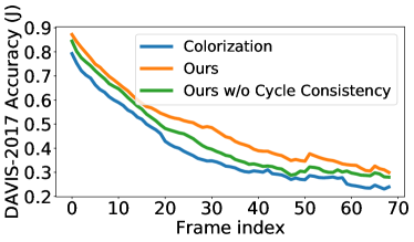
Cycle Consistency Lastly, we evalute the effectiveness of forward-backward consistency. As seen in Figure 5, while both models start off with high accuracy early in a video sequence, the model with cycle-consistency maintains a higher performance in later stages of video sequences, indicating a less severe drifting problem. This can also be reflected in the quantitative analysis, where cycle consistency enables a performance boost by in and in .
4.1.2 Comparison with State-of-the-art
In Table 1, we show comparisons with previous approaches on the DAVIS-2017 video segmentation benchmark. Three phenomena can be observed: First, Our model clearly dominates all the self-supervised method, surpassing both video colourization ( vs. on &) and CycleTime ( vs. on &). Second, our model outperforms the optical flow method significantly, suggesting the colour dropout and scheduled sampling has improved the model’s robustness under scenarios that optical flow is deemed to fail, e.g\bmvaOneDotlarge illunimation changes. Third, our model trained with self-supervised learning can even approach the results of some supervised methods, for instance, despite of only using a ResNet18 as feature encoder, the results are comparable with the ResNet50 pretrained on ImageNet ( vs. on &). We conjecture this is due to the fact that the model pretrained with ImageNet has only encoded high-level semantics, while not optimized for dense correspondence matching.
4.1.3 Accuracy by Attributes
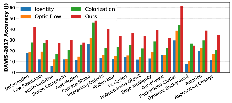
In Figure 6, we show DAVIS-2017 testing accuracy grouped into different categories. The proposed method has shown to outperform the previous methods in all situations, suggesting that our model has learned better feature embeddings for robust correspondence flow.
4.1.4 Qualitative Results
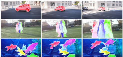
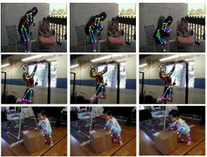
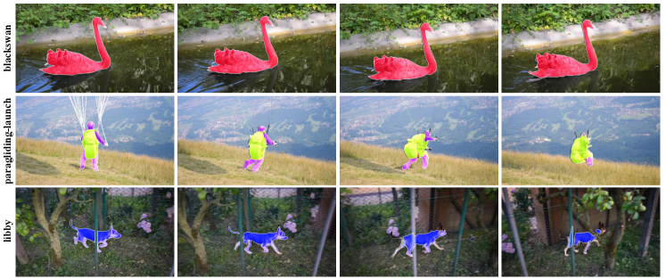
As shown in Figure 1 and Figure 7, we provide the qualitative prediction from our model. The segmentation mask can be propagated through sequences even when facing large scale variation from camera motion, and object deformations.
4.1.5 Probing Upper Bound of Self-supervised Learning
Despite the superior performance on video segmentation, we notice that training models on Kinetics is not ideal, as it is a human-centric video dataset. However, most of the classes in DAVIS are not covered by Kinetics, e.g\bmvaOneDotcars, animals.
To shed light on the potential of self-supervised learning on the task of correspondence flow, we probe the upper bound by training on more diverse video data. We randomly pick DAVIS classes and download additional videos from YouTube, and further train the model by varying the amount of additional data. Note that, we only download videos by the class labels, and no segmentation annotations are provided during further self-supervised training.
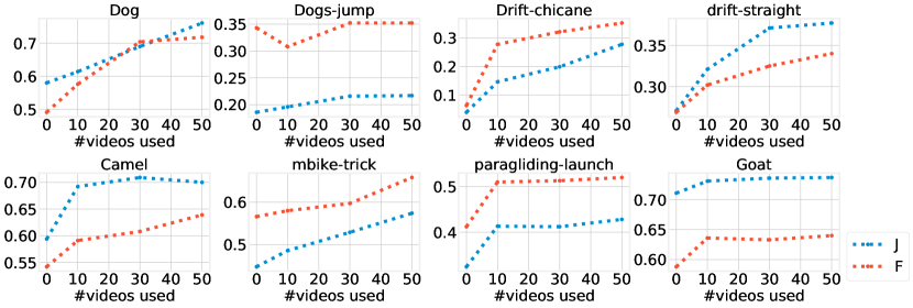
As shown in Figure 8 and Table 2, two phenomena can be observed: First, as the number of additional training videos increases (Figure 8), all sequences have seen a performance boost on both metrics (). Second, the segmentation on some of the classes are even comparable or surpassing the supervised learning, e.g\bmvaOneDotDrift-c, Camel, Paragliding. We conjecture this is due to the fact that, there are only very limited manual annotations for these classes for supervised learining, e.g\bmvaOneDotParagliding. However, with self-supervised learning, we only require raw video data which is almost infinite.
| Method | Dataset | Dog | Dog-j | Drift-c | Drift-s | Camel | Mbike | Paragliding | Goat |
|---|---|---|---|---|---|---|---|---|---|
| Self-supervised () | Kinetics | 58.0 | 18.6 | 3.9 | 27.1 | 59.4 | 44.8 | 32.4 | 71.1 |
| Self-supervised () | Additional | 76.1 | 21.7 | 27.8 | 37.7 | 70.0 | 57.4 | 42.8 | 73.7 |
| Supervised () [Yang et al.(2018)Yang, Wang, Xiong, Yang, and Katsaggelos] | COCO+DAVIS | 87.7 | 38.8 | 4.9 | 66.4 | 88.4 | 72.5 | 38.0 | 80.4 |
| Self-supervised () | Kinetics | 49.1 | 34.3 | 6.3 | 26.9 | 54.2 | 56.6 | 41.2 | 58.8 |
| Self-supervised () | Additional | 71.8 | 35.2 | 35.3 | 34.0 | 63.9 | 65.8 | 52.0 | 64.0 |
| Supervised () [Yang et al.(2018)Yang, Wang, Xiong, Yang, and Katsaggelos] | COCO+DAVIS | 84.6 | 45.2 | 8.4 | 57.7 | 92.2 | 76.7 | 58.1 | 74.7 |
4.2 Keypoint Tracking on JHMDB
As shown in Table 3, our approach exceeds the previous methods [Vondrick et al.(2018)Vondrick, Shrivastava, Fathi, Guadarrama, and Murphy] by an average of in PCKinstance. Also, we achieve better performance in the more strict PCK@.1 metric when compared to the recent work [Wang et al.(2019b)Wang, Jabri, and Efros]. Interestingly, when taking the benefit of the almost infinite amount of video data, self-supervised learning methods (CycleTime and Ours) achieve comparable or even outperforms model trained with the supervised learning[He et al.(2016)He, Zhang, Ren, and Sun, Song et al.(2017)Song, Wang, Van Gool, and Hilliges].
| Method | Supervised | Dataset | PCKinstance | PCKmax | |||
| @.1 | @.2 | @.1 | @.2 | ||||
| SIFT Flow[Liu et al.(2011)Liu, Yuen, and Torralba] | ✗ | - | 49.0 | 68.6 | - | - | |
| Video Colorization [Vondrick et al.(2018)Vondrick, Shrivastava, Fathi, Guadarrama, and Murphy] | ✗ | Kinetics | 45.2 | 69.6 | - | - | |
| CycleTime (ResNet-50) [Wang et al.(2019b)Wang, Jabri, and Efros] | ✗ | VLOG | 57.7 | 78.5 | - | - | |
| Ours (Full Model ResNet-18) | ✗ | Kinetics | 58.5 | 78.8 | 71.9 | 88.3 | |
| ImageNet (ResNet-50) [He et al.(2016)He, Zhang, Ren, and Sun] | ✓ | ImageNet | 58.4 | 78.4 | - | - | |
| Fully Supervised [Song et al.(2017)Song, Wang, Van Gool, and Hilliges] | ✓ | JHMDB | - | - | 68.7 | 81.6 | |
5 Conclusion
The paper aims to explore the self-supervised learning for pixel-level correspondence matching in videos. We proposed a simple information bottleneck that enables the model to be trained on standard RGB images, and nicely close the gap between training and testing. To alleviate the challenge from model drifting, we formulate the model in a recursive manner, trained with scheduled sampling and forward-backward cycle consistency. We demonstrate state-of-the-art performance on video segmentation and keypoint tracking. To further shed light on the potential of self-supervised learning on correspondence flow, we probe the upper bound by training on additional and more diverse video datasets, and show that self-supervised learning for correspondence flow is far from being saturated. As future work, potential extensions can be: First, explore better approaches for overcoming tracker drifting, e.g\bmvaOneDotuse explicit memory modules for long-term correspondence flow. Second, define robust loss functions that can better handle complex object deformation and occlusion, e.g\bmvaOneDotpredicting visibility mask or apply losses at feature level [Oord et al.(2018)Oord, Li, and Vinyals]. Third, instead of doing quantization with Kmeans clustering, train the quantization process to be more semantically meaningful.
Acknowledgment
Financial support for this project is provided by EPSRC Seebibyte Grant EP/M013774/1.
References
- [Agrawal et al.(2015)Agrawal, Carreira, and Malik] P. Agrawal, J. Carreira, and J. Malik. Learning to see by moving. In Proc. ICCV, 2015.
- [Bailer et al.(2017)Bailer, Varanasi, and Stricker] C. Bailer, K. Varanasi, and D. Stricker. Cnn-based patch matching for optical flow with thresholded hinge embedding loss. In Proc. CVPR, 2017.
- [Bengio et al.(2015)Bengio, Vinyals, Jaitly, and Shazeer] S. Bengio, O. Vinyals, N. Jaitly, and N. Shazeer. Scheduled sampling for sequence prediction with recurrent neural networks. In NIPS, 2015.
- [Brox et al.(2004)Brox, Bruhn, Papenberg, and Weickert] T. Brox, A. Bruhn, N. Papenberg, and J. Weickert. High accuracy optical flow estimation based on a theory for warping. In Proc. ECCV, 2004.
- [Brox et al.(2009)Brox, Bregler, and Malik] T. Brox, C. Bregler, and J. Malik. Large displacement optical flow. In Proc. CVPR, 2009.
- [Caelles et al.(2017)Caelles, Maninis, Pont-Tuset, Leal-Taixé, Cremers, and Van Gool] S. Caelles, K.K Maninis, J. Pont-Tuset, L. Leal-Taixé, D. Cremers, and L. Van Gool. One-shot video object segmentation. In Proc. CVPR, 2017.
- [Denton and Birodkar(2017)] E.L. Denton and V. Birodkar. Unsupervised learning of disentangled representations from video. In NIPS, 2017.
- [Dosovitskiy et al.(2015)Dosovitskiy, Fischer, Ilg, Hausser, Hazirbas, Golkov, Smagt, Cremers, and Brox] A. Dosovitskiy, P. Fischer, E. Ilg, P. Hausser, C. Hazirbas, V. Golkov, P. Smagt, D. Cremers, and T. Brox. Flownet: Learning optical flow with convolutional networks. In Proc. ICCV, 2015.
- [Fernando et al.(2017)Fernando, Bilen, Gavves, and Gould] B. Fernando, H. Bilen, E. Gavves, and S. Gould. Self-supervised video representation learning with odd-one-out networks. In CVPR, 2017.
- [Gan et al.(2018)Gan, Gong, Liu, Su, and Guibas] C. Gan, B. Gong, K. Liu, H. Su, and L. J. Guibas. Geometry guided convolutional neural networks for self-supervised video representation learning. In Proc. CVPR, 2018.
- [Han et al.(2017)Han, Rezende, Ham, Wong, Cho, Schmid, and Ponce] K. Han, R.S. Rezende, B. Ham, K.Y.K. Wong, M. Cho, C. Schmid, and J. Ponce. Scnet: Learning semantic correspondence. In Proc. ICCV, 2017.
- [Hartley and Zisserman(2004)] R. I. Hartley and A. Zisserman. Multiple View Geometry in Computer Vision. Cambridge University Press, second edition, 2004.
- [He et al.(2016)He, Zhang, Ren, and Sun] K. He, X. Zhang, S. Ren, and J. Sun. Deep residual learning for image recognition. In Proc. CVPR, 2016.
- [Horn and Schunck(1981)] B. K. P. Horn and B. G. Schunck. Determining optical flow. Artificial Intelligence, 17:185–203, 1981.
- [Ilg et al.(2017)Ilg, Mayer, Saikia, Keuper, Dosovitskiy, and Brox] E. Ilg, N. Mayer, T. Saikia, M. Keuper, A. Dosovitskiy, and T. Brox. Flownet 2.0: Evolution of optical flow estimation with deep networks. In Proc. CVPR, 2017.
- [Isola et al.(2015)Isola, Zoran, Krishnan, and Adelson] P. Isola, D. Zoran, D. Krishnan, and E.H. Adelson. Learning visual groups from co-occurrences in space and time. In Proc. ICLR, 2015.
- [Jakab et al.(2018)Jakab, Gupta, Bilen, and Vedaldi] T. Jakab, A. Gupta, H. Bilen, and A. Vedaldi. Conditionalimagegenerationforlearning the structure of visual objects. In NIPS, 2018.
- [Jayaraman and Grauman(2015)] D. Jayaraman and K. Grauman. Learning image representations tied to ego-motion. In Proc. ICCV, 2015.
- [Jayaraman and Grauman(2016)] D. Jayaraman and K. Grauman. Slow and steady feature analysis: higher order temporal coherence in video. In Proc. CVPR, 2016.
- [Jia et al.(2016)Jia, De Brabandere, and Tuytelaars] X. Jia, B. De Brabandere, and T. Tuytelaars. Dynamic filter networks. In NIPS, 2016.
- [Jia et al.(2017)Jia, Ranftl, and Koltun] X. Jia, R. Ranftl, and V. Koltun. Accurate optical flow via direct cost volume processing. In Proc. CVPR, 2017.
- [Jing and Tian(2018)] L. Jing and Y. Tian. Self-supervised spatiotemporal feature learning by video geometric transformations. arXiv preprint arXiv:1811.11387, 2018.
- [Kay et al.(2017)Kay, Carreira, Simonyan, Zhang, Hillier, Vijayanarasimhan, F., Green, Natsev, Suleyman, and Zisserman] W. Kay, J. Carreira, K. Simonyan, B. Zhang, C. Hillier, S. Vijayanarasimhan, Viola F., T. Green, P. Natsev, M. Suleyman, and A. Zisserman. The kinetics human action video dataset. 2017.
- [Kendall et al.(2017)Kendall, Martirosyan, Dasgupta, Henry, Kennedy, Bachrach, and Bry] A. Kendall, H. Martirosyan, S. Dasgupta, P. Henry, R. Kennedy, A. Bachrach, and A. Bry. End-to-end learning of geometry and context for deep stereo regression. In Proc. CVPR, 2017.
- [Kim et al.(2018)Kim, Cho, and Kweon] D. Kim, D. Cho, and I. S. Kweon. Self-supervised video representation learning with space-time cubic puzzles. In AAAI, 2018.
- [Kim et al.(2017)Kim, Min, Ham, Jeon, Lin, and Sohn] S. Kim, D. Min, B. Ham, S. Jeon, S. Lin, and K. Sohn. Fcss: Fully convolutional self-similarity for dense semantic correspondence. In Proc. CVPR, 2017.
- [Lee et al.(2017)Lee, Huang, Singh, and Yang] H.Y. Lee, J.B. Huang, M. Singh, and M.H. Yang. Unsupervised representation learning by sorting sequences. In Proc. ICCV, 2017.
- [Liu et al.(2011)Liu, Yuen, and Torralba] C. Liu, J. Yuen, and A. Torralba. Sift flow: Dense correspondence across scenes and its applications. IEEE transactions on pattern analysis and machine intelligence, 2011.
- [Meister et al.(2018)Meister, Hur, and Roth] S. Meister, J. Hur, and S. Roth. UnFlow: Unsupervised learning of optical flow with a bidirectional census loss. In AAAI, 2018.
- [Misra et al.(2016)Misra, Zitnick, and Hebert] I. Misra, C. L. Zitnick, and M. Hebert. Shuffle and learn: Unsupervised learning using temporal order verification. In ECCV, 2016.
- [Novotny et al.(2017)Novotny, Larlus, and Vedaldi] D. Novotny, D. Larlus, and A. Vedaldi. Anchornet: A weakly supervised network to learn geometry-sensitive features for semantic matching. In Proc. CVPR, 2017.
- [Oord et al.(2018)Oord, Li, and Vinyals] A.v.d. Oord, Y. Li, and O. Vinyals. Representation learning with contrastive predictive coding. arXiv preprint arXiv:1807.03748, 2018.
- [Pont-Tuset et al.(2017)Pont-Tuset, F., Caelles, Arbeláez, Sorkine-Hornung, and Van Gool] J. Pont-Tuset, Perazzi. F., S. Caelles, P. Arbeláez, A. Sorkine-Hornung, and L. Van Gool. The 2017 davis challenge on video object segmentation. arXiv:1704.00675, 2017.
- [Revaud et al.(2015)Revaud, Weinzaepfel, Harchaoui, and Schmid] J. Revaud, P. Weinzaepfel, Z. Harchaoui, and C. Schmid. Epicflow: Edge-preserving interpolation of correspondences for optical flow. In Proc. CVPR, 2015.
- [Rocco et al.(2017)Rocco, Arandjelovic, and Sivic] I. Rocco, R. Arandjelovic, and J. Sivic. Convolutional neural network architecture for geometric matching. In Proc. CVPR, 2017.
- [Rocco et al.(2018)Rocco, Arandjelovic, and Sivic] I. Rocco, R. Arandjelovic, and J. Sivic. End-to-end weakly-supervised semantic alignment. In Proc. CVPR, 2018.
- [Smith and Brady(1995)] S.M. Smith and J.M. Brady. Asset-2: Real-time motion segmentation and shape tracking. IEEE Transactions on Pattern Analysis and Machine Intelligence, 17(8):814–820, 1995.
- [Song et al.(2017)Song, Wang, Van Gool, and Hilliges] J. Song, L. Wang, L. Van Gool, and O. Hilliges. Thin-slicing network: A deep structured model for pose estimation in videos. In Proc. CVPR, 2017.
- [Valmadre et al.(2018)Valmadre, Bertinetto, Henriques, R., Vedaldi, Smeulders, Torr, and Gavves] J. Valmadre, L. Bertinetto, J. F. Henriques, Tao R., A. Vedaldi, A. Smeulders, P. H. S. Torr, and E. Gavves. Long-term tracking in the wild: A benchmark. In ECCV, 2018.
- [Vondrick et al.(2018)Vondrick, Shrivastava, Fathi, Guadarrama, and Murphy] C. Vondrick, A. Shrivastava, A. Fathi, S. Guadarrama, and K. Murphy. Tracking emerges by colorizing videos. In Proc. ECCV, 2018.
- [Wang et al.(2019a)Wang, Zhang, Bertinetto, Hu, and Torr] Q. Wang, L. Zhang, L. Bertinetto, W. Hu, and P.H.S Torr. Fast online object tracking and segmentation: A unifying approach. In Proc. CVPR, 2019a.
- [Wang et al.(2017)Wang, He, and Gupta] X. Wang, K. He, and A. Gupta. Transitive invariance for self-supervised visual representation learning. In Proc. CVPR, 2017.
- [Wang et al.(2019b)Wang, Jabri, and Efros] X. Wang, A. Jabri, and A. Efros. Learning correspondence from the cycle-consistency of time. In Proc. CVPR, 2019b.
- [Wang and Gupta(2015)] X.L Wang and A. Gupta. Unsupervised learning of visual representations using videos. In ICCV, 2015.
- [Wang et al.(2018)Wang, Yang, Yang, Zhao, Wang, and Xu] Y. Wang, Y. Yang, Z. Yang, L. Zhao, P. Wang, and W. Xu. Occlusion aware unsupervised learning of optical flow. In Proc. CVPR, 2018.
- [Wei et al.(2018)Wei, Lim, Zisserman, and Freeman] D.L. Wei, J.J. Lim, A. Zisserman, and W.T. Freeman. Learning and using the arrow of time. In CVPR, 2018.
- [Weinzaepfel et al.(2013)Weinzaepfel, Revaud, Harchaoui, and Schmid] P. Weinzaepfel, J. Revaud, Z. Harchaoui, and C. Schmid. DeepFlow: Large displacement optical flow with deep matching. In Proc. ICCV, pages 1385–1392, 2013.
- [Wiles et al.(2018)Wiles, Koepke, and Zisserman] O. Wiles, A.S. Koepke, and A. Zisserman. X2face: A network for controlling face generation using images, audio, and pose codes. In Proc. ECCV, 2018.
- [Wiskott and Sejnowski(2002)] L. Wiskott and T. Sejnowski. Slow feature analysis: Unsupervised learning of invariances. In Neural Computation, 2002.
- [Xie et al.(2016)Xie, Girshick, and Farhadi] J. Xie, R. Girshick, and A. Farhadi. Unsupervised deep embedding for clustering analysis. In Proc. ICML, 2016.
- [Yang et al.(2018)Yang, Wang, Xiong, Yang, and Katsaggelos] L. Yang, Y. Wang, X. Xiong, J. Yang, and A. K. Katsaggelos. Efficient video object segmentation via network modulation. In Proc. CVPR, 2018.
- [Yu et al.(2016)Yu, Harley, and Derpanis] J.J. Yu, A.W. Harley, and K.G. Derpanis. Back to basics: Unsupervised learning of optical flow via brightness constancy and motion smoothness. In Proc. ECCV, 2016.
Appendix A Network Architecture
We use a modified ResNet-18[He et al.(2016)He, Zhang, Ren, and Sun] architecture with enlarged output feature maps size. Details of the network can be found below.
| 0 | Input image |
|---|---|
| Feature extractor | |
| 1 | conv with stride 2 and 64 filters |
| 2 | Residual Block with stride 1 and 64 filters |
| 3 | Residual Block with stride 2 and 128 filters |
| 4 | Residual Block with stride 1 and 256 filters |
| 5 | Residual Block with stride 1 and 256 filters |
A.1 Failure Cases
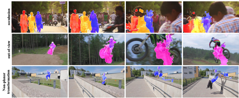
Figure 9 demonstrates some failure cases during mask propagation. Row 1 shows our tracker fails due to occlusions. As we only use the mask of the previous frame to propagate, an object is unlikely to be retrieved after it has been occluded. Similarly, it is difficult to recover an object once it goes out of the frame (Row 2). Lastly, if the object is under complex deformation, it is likely to incur the model drifting.
