Weight Map Layer for Noise and Adversarial Attack Robustness
Abstract
Convolutional neural networks (CNNs) are known for their good performance and generalization in vision-related tasks and have become state-of-the-art in both application and research-based domains. However, just like other neural network models, they suffer from a susceptibility to noise and adversarial attacks. An adversarial defence aims at reducing a neural network’s susceptibility to adversarial attacks through learning or architectural modifications. We propose the weight map layer (WM) as a generic architectural addition to CNNs and show that it can increase their robustness to noise and adversarial attacks. We further explain that the enhanced robustness of the two WM variants results from the adaptive activation-variance amplification exhibited by the layer. We show that the WM layer can be integrated into scaled up models to increase their noise and adversarial attack robustness, while achieving comparable accuracy levels across different datasets.
1 Introduction
Despite their wide adoption in vision tasks and practical applications, convolutional neural networks (CNNs) (Fukushima and Miyake, 1980; LeCun et al., 1989; Krizhevsky et al., 2012) suffer from the same noise susceptibility problems manifested in the majority of neural network models. Noise is an integral component of any input signal that can arise from different sources, from sensors and data acquisition to data preparation and pre-processing. Szegedy et al. (2013) opened the door to an extreme set of procedures that can manipulate this susceptibility by applying an engineered noise to confuse a neural network to misclassify its inputs.
The core principle in this set of techniques, called adversarial attacks, is to apply the least possible noise perturbation to the neural network input, such that the noisy input is not visually distinguishable from the original and yet it still disrupts the neural network output. Generally, adversarial attacks are composed of two main steps:
-
•
Direction sensitivity estimation: In this step, the attacker estimates which directions in the input are the most sensitive to perturbation. In other words, the attacker finds which input features will cause the most degradation of the network performance when perturbed. The gradient of the loss with respect to the input can be used as a proxy of this estimate.
-
•
Perturbation selection: Based on the sensitivity estimate, some perturbation is selected to balance the two competing objectives of being minimal and yet making the most disruption to the network output.
The above general technique implies having access to the attacked model and thus is termed a whitebox attack. Blackbox attacks on the other hand assume no access to the target model and usually entail training a substitute model to approximate the target model and then applying the usual whitebox attack (Chakraborty et al., 2018). The effectiveness of this approach mainly depends on the assumption of the transferability between machine learning models (Papernot et al., 2016a).
Since their introduction, a lot of research have been done to guard against these attacks. An adversarial defence is any technique that is aimed at reducing the effect of adversarial attacks on neural networks. This can be through detection, modification to the learning process, architectural modifications or a combination of these techniques. Our approach consists of an architectural modification that aims to be easily integrated into any existing convolutional neural network architecture.
The core hypothesis we base our approach on starts from the premise that the noise in an input is unavoidable and in practise is very difficult to separate from the signal effectively. Instead, if the network can adaptively amplify the features activation variance selectively in its representations based on their importance, then it can absorb the variation introduced by the noise and map the representations to the correct output. This means that if a feature is very important to the output calculation, then its activation and intrinsic noise should be adequately amplified at training time to allow the classification layers to be robust to this feature’s noisiness at inference time, since it is crucial to performance. In the context of CNNs, this kind of feature-wise amplification can be achieved by an adaptive elementwise scaling of feature maps.
We introduce the weight map layer (WM), which is an easy to implement layer composed of two main operations: elementwise scaling of feature maps by a learned weight grid of the same size, followed by a non-adaptive convolution reduction operation. We use two related operations in the two WM variants we introduce. The first variant, smoothing WM, uses a non-adaptive smoothing convolution filter of ones. The other variant, unsharp WM, adds an extra step to exploit the smoothed intermediate output of the first variant to implement an operation similar to unsharp mask filtering (Gonzalez et al., 2002). The motivation for the second variant was to decrease the over-smoothing effect produced by stacking multiple WM layers. Smoothing is known to reduce adversarial susceptibility (Xu et al., 2017), however if done excessively this can negatively impact accuracy, which motivates the unsharp operation as a counter-measure to help control the trade-off between noise robustness and overall accuracy. We show and argue that the weight map component, can increase robustness to noise by amplifying the noise during the training phase in an adaptive way based on feature importance and, hence, can help networks absorb noise more effectively. In a way, this can be thought of as implicit adversarial training (Goodfellow et al., 2014; Lyu et al., 2015; Shaham et al., 2015). We show that the two components, weight map and reduction operations, can give rise to robust CNNs that are resistant to uniform and adversarial noise.
2 Related Work
Since the intriguing discovery by Szegedy et al. (2013) that neural networks can be easily forced to misclassify their input by applying an imperceptible perturbation, many attempts have been made to fortify them against such attacks. These techniques are generally applied to either learning or architectural aspects of networks. Learning techniques modify the learning process to make the learned model resistant to adversarial attacks, and are usually architecture agnostic. Architectural techniques, on the other hand, make modifications to the architecture or use a specific form of architecture engineered to exhibit robustness to such attacks.
Goodfellow et al. (2014) suggested adversarial training, where the neural network model is exposed to crafted adversarial examples during the training phase to allow the network to map adversarial examples to the right class. Tramèr et al. (2017) showed that this can be bypassed by a two step-attack, where a random step is applied before perturbation. Jin et al. (2015) used a similar approach of training using noisy inputs, with some modifications to network operators to increase robustness to adversarial attacks. Seltzer et al. (2013) also applied a similar technique in the audio domain, namely, multi-condition speech, where the network is trained on samples with different noise levels. They also benchmarked against training on pre-processed noise-suppressed features and noise-aware training, a technique where the input is augmented with noise estimates.
Distillation (Hinton et al., 2015) was proposed initially as a way of transferring knowledge from a larger teacher network to a smaller student network. One of the tricks used to make distillation feasible was the usage of softmax with a temperature hyperparameter. Training the teacher network with a higher temperature has the effect of producing softer targets that can be utilized for training the student network. Papernot et al. (2016b); Papernot and McDaniel (2017) showed that distillation with a high temperature hyperparameter can render the network resistant to adversarial attacks. Feature squeezing (Xu et al., 2017) corresponds to another set of techniques that rely on desensitizing the model to input, e.g. through smoothing images, so that it is more robust to adversarial attacks. This, however, decreases the model’s accuracy. Hosseini et al. (2017) proposed NULL labeling, where the neural network is trained to reject inputs that are suspected to be adversarials.
Sinha et al. (2018) proposed using adversarial networks to train the target network using gradient reversal (Ganin et al., 2015). The adversarial network is trained to classify based on the loss derived gradient, so that the confusion between classes with similar gradients is decreased. Pontes-Filho and Liwicki (2018) proposed bidirectional learning, where the network is trained as a classifier and a generator, with an associated adversarial network, in two different directions and found that it renders the trained classifier more robust to adversarial attacks.
From the architectural family, Lamb et al. (2018) proposed inserting Denoising Autoencoders (DAEs) between hidden layers. They act as regularizers for different hidden layers, effectively correcting representations that deviate from the expected distribution. A related approach was proposed by Ghosh et al. (2018), where a Variational Autoencoder (VAE) was used with a mixture of Gaussians prior. The adversarial examples could be detected at inference time based on their high reconstruction errors and could then be correctly reclassified by optimizing for the latent vector that minimized the reconstruction error with respect to the input. DeepCloak (Gao et al., 2017) is another approach that accumulates the difference in activations between the adversarials and the seeds used to generate them at inference time and, based on this, a binary mask is inserted between hidden layers to zero out the features with the highest contribution to the adversarial problem. The nearest to our approach, is the method proposed by Sun et al. (2017). This work made use of a HyperNetwork (Ha et al., 2016) that receives the mean and standard deviation of the convolution layer and outputs a map that is multiplied elementwise with the convolution weights to produce the final weights used to filter the input. The dependency of the weights on the statistics of the data renders the network robust to adversarial attacks.
We introduce the WM layer, an adversarial defence which requires a minimal architectural modification since it can be inserted between normal convolutional layers. We propose that the adaptive activation-variance amplification achieved by the layer, which can be considered as a form of dynamic implicit adversarial training, can render CNNs robust to different forms of noise. Finally, we show that the WM layer can be integrated into scaled up models to achieve noise robustness with the same or similar accuracy in many cases across different datasets.
3 Methods
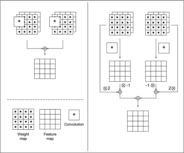
The main operation involved in a weight map layer fig. 1 is an elementwise multiplication of the layer input with a map of weights. For a layer with an input with input channels and spatial dimension and an output with output channels and spatial dimension, the channel map of the th input channel contributing to the th output channel is calculated as
| (1) |
where is the weight mapping between and , is the th input channel and is the elementwise multiplication operator. We used two techniques for producing the pre-nonlinearity output of the weight map layer. The first variant, smoothing weight map layer, produces the th output channel by convolving the maps with a kernel of ones with spatial dimension as follow,
| (2) |
where is the set of intermediate maps contributing to output channel , is a bias term and is the convolution operator. The other variant, unsharp weight map layer, produces the output by an operation similar to unsharp filtering as follow,
| (3) |
| (4) |
where is a kernel of ones applied with a suitable padding element to ensure similar spatial dimensions between the convolution input and output.
4 Experiments
| Layer | CNN | CNN (wide) | WM |
|---|---|---|---|
| 1 | Conv(33 channels) | Conv(200 channels) | WM (32 channels) |
| 2 | Conv(33 channels) | Conv(500 channels) | WM (32 channels) |
| 3 | Conv(8 channels) | Conv(8 channels) | WM (8 channels) |
| 4 | FC(64 nodes) | FC(64 nodes) | FC(64 nodes) |
| 5 | FC(10 nodes) | FC(10 nodes) | FC(10 nodes) |
| Layer | Out dimension | Repeat |
|---|---|---|
| ResBlock | 8 | 3 |
| ResBlock | 16 | 4 |
| ResBlock | 32 | 6 |
| ResBlock | 64 | 4 |
| Global average pool | 64 | 1 |
| Fully connected | 10 | 1 |
| Layer | Hyperparams | Repeat |
|---|---|---|
| Conv | channels: 16 | 1 |
| ReLU | channels: 16 | 1 |
| Dense | Growth rate: 8 | 2 |
| Max pool | size:2, stride:2 | 1 |
| Dense | Growth rate: 8 | 4 |
| Max pool | size:2, stride:2 | 1 |
| Dense | Growth rate: 8 | 8 |
| Max pool | size:2, stride:2 | 1 |
| Dense | Growth rate: 8 | 16 |
| Global average pool | out: 256 | 1 |
| Fully connected | out: 10 | 1 |
We tested our method on three architectures and three datasets. For every dataset, we benchmark a number of weight-map layer variants against a baseline. The baseline and the variants share the same skeleton, but the layers in the baseline are convolutional layers, while in the different weight map variants some or all of the convolutional layers are replaced with a variant of the weight map layer. We train each model for 300 epochs using the Adam optimizer. The test error reported on the non-noisy dataset is an average of three trials. For the weight map layer, we initialize the weights and biases according to
where U is the normal distribution and is the fan-in.
In the preliminary experiments on the MNIST dataset, we tested three different architectures: CNN, ResNet (He et al., 2015) and DenseNet (Huang et al., 2016) and for the two other datasets (CIFAR10 and iWild Cam2019) we tested ResNet and DenseNet. The CNN skeleton is a stack of three layers, where the first two have either 32 channels, if it is a weight map network variant, or 33 channels if it is a normal CNN table 1. This difference was adopted to maintain approximately the same number of floating point operations per second (FLOPS) between the two architectures. In just one of the CNN variants, we increased the channels of the first two layers to 200 and 500, respectively, to compare with the weight map network having the same number of parameters. We will refer to this scaled up variant as "wide" in the results. The final layer in the skeleton body has 8 channels. Classification output is made by a 2 layer fully connected multilayer perceptron (MLP), where the first layer has 64 nodes followed by an output layer. We fixed the kernel size across all the layers. We compare two kernel sizes, 3 and 9, and we include batchnorm (Ioffe and Szegedy, 2015) layers in some of the variants to test the interaction with the proposed layer. When batchnorm is included, it is inserted in all the convolutional layers just before the nonlinearity. In one of the variants, we elementwise multiply the input with a learned weight map to probe the effect of the input weight map on noise robustness.
To assess the scalability of the proposed weight map layer, we integrated it into two popular CNN skeletons: ResNet and DenseNet. Table 2 shows the skeleton of the ResNet variant. ResBlock was composed of two layers of 3x3 convolutions with ReLU activations. At layer transitions characterized by doubling of the number of channels, downsampling to half of the spatial dimension was done by the first layer of the first block. Residual connections were established from the input to each ResBlock to its output, following the pattern used in the original paper (He et al., 2015), where projections using 1x1 convolutions were applied when there was a mismatch of the number of channels or spatial dimensions. Table 3 shows the skeleton of DenseNet. Each Dense layer is assumed to be followed by a ReLU nonlinearity. For integrating WM layers into the architectures, we either replace all the layers by one of the WM layer variants or replace half of the layers by skipping one layer and replacing the next. We will refer to the former by the non-alternating WM model and to the latter by the alternating WM model.
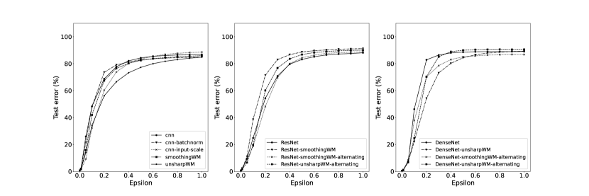
We tested model robustness on two types of noise, uniform noise and adversarial noise. When testing models for uniform noise robustness, we added random uniform noise to the input, which always had a lower boundary of zero. We varied the upper boundary to assess the degree of robustness. After the addition of the noise, the input was renormalized to be within the range . The robustness measure is reported as the average test error achieved by the model on the noisy test dataset averaged over three trials. For testing the models against adversarial attacks, we followed the fast gradient sign method (FSGM) (Goodfellow et al., 2014) approach, where we varied the parameter to control the severity of the attack.
4.1 MNIST
The MNIST dataset is a collection of images of handwritten digits with 10 classes representing the digits from 0 to 9. The images are grayscale with spatial dimensions of 28x28. MNIST consists of a training dataset of 60k samples and a testing dataset of 10k samples. We divide the training dataset into 90% for training and 10% for validation. The only augmentation used during the training was padding by 2 and then random cropping a 28x28 patch. The test dataset was used as it is. The results on MNIST are summarized in table 5 and fig. 2.
4.2 CIFAR10
The CIFAR10 dataset is a collection of colored (3-channels) images comprising 10 classes representing animals and vehicles. The images have 32x32 spatial dimensions. CIFAR10 consists of 50k training images and 10k testing images. We divide the training set into 90% for training and 10% for validation. No augmentation was used for the training data. The test dataset was used as it is. CIFAR10 results are summarized in table 6 and fig. 3.
4.3 iWildCam2019
The iWildCam2019 dataset is a collection of colored animal images captured in the wild by camera traps. The dataset is imbalanced and there is only a partial overlap between the classes found in the training and test datasets. To balance the dataset and fix the classes between training and testing, we used only the training set by splitting it into training, validation and test sets. This was done by first choosing 10 classes (deer, squirrel, rodent, fox, coyote, raccoon, skunk, cat, dog, opossum), then balancing all the classes by choosing only 1000 samples from each class. We then split the data into 70% training, 20% validation and 10% test. This was done class-wise to maintain the balance. We preprocessed all the sets by converting the images to grayscale and downsampling to 23x32 spatial dimensions. No augmentation was used. iWildCam2019 results are summarized in table 7 and fig. 4.
4.4 Results
| Arch | Variant | Params | GFLOPS | Test error (%) |
|---|---|---|---|---|
| CNN | wide | 1.19M | 1.07 | |
| CNN | 33 channels | 261K | 0.014 | |
| CNN | 33 channels - batchnorm | 261K | 0.014 | |
| CNN | 33 channels - kernel size 9 | 361K | 0.125 | |
| CNN | 33 channels - input-scale | 261K | 0.014 | |
| Smooth WM | 32 channels | 1.16M | 0.013 | |
| Smooth WM | 32 channels - batchnorm | 1.16M | 0.013 | |
| Smooth WM | 32 channels - kernel size 9 | 1.16M | 0.119 | |
| Unsharp WM | 32 channels | 1.49M | 0.020 |
| Variant | Test error (%) |
|---|---|
| ResNet | |
| Conv | |
| Smoothing WM | |
| Unsharp WM | |
| Alternating Conv/Smoothing WM | |
| Alternating Conv/Unsharp WM | |
| DenseNet | |
| Conv | |
| Smoothing WM | |
| Unsharp WM | |
| Alternating Conv/Smoothing WM | |
| Alternating Conv/Unsharp WM | |
| Variant | Test error (%) |
|---|---|
| ResNet | |
| Conv | |
| Alternating Conv/Smoothing WM | |
| Alternating Conv/Unsharp WM | |
| DenseNet | |
| Conv | |
| Alternating Conv/Smoothing WM | |
| Alternating Conv/Unsharp WM | |
| Variant | Test error (%) |
|---|---|
| ResNet | |
| Conv | |
| Alternating Conv/Smoothing WM | |
| Alternating Conv/Unsharp WM | |
| DenseNet | |
| Conv | |
| Alternating Conv/Smoothing WM | |
| Alternating Conv/Unsharp WM | |
The test errors of the preliminary experiments benchmarking CNN on MNIST are summarized in table 4. The basic weight map network has better performance than the corresponding basic CNN with the same number of FLOPS. The unsharp version is better by a larger margin but with slightly higher FLOPS. Increasing the CNN parameters to the level of the corresponding weight map network results in lowering its performance. Including batchnorm in either the CNN or the weight map network boosted the performance of both variants to nearly the same level. On the other hand, increasing the kernel size to 9 boosted the CNN performance, whilst degrading the weight map network performance.
The test error results of ResNet and DenseNet are summarized in table 5, table 6 and table 7. Baseline ResNet had better performance than the weight map layer variants on MNIST and CIFAR10, while all of the weight map layer variants were better than the baseline on iWildCam2019. For DenseNet tested on MNIST, the baseline had better performance than the non-alternating weight map layer variants, while it had similar performance to the alternating variants. On iWildCam2019, the baseline DenseNet had similar performance to the alternating smoothing variant and lower performance than the alternating unsharp variant. On CIFAR10, the weight map variants had lower performance than the baseline DenseNet.
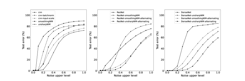
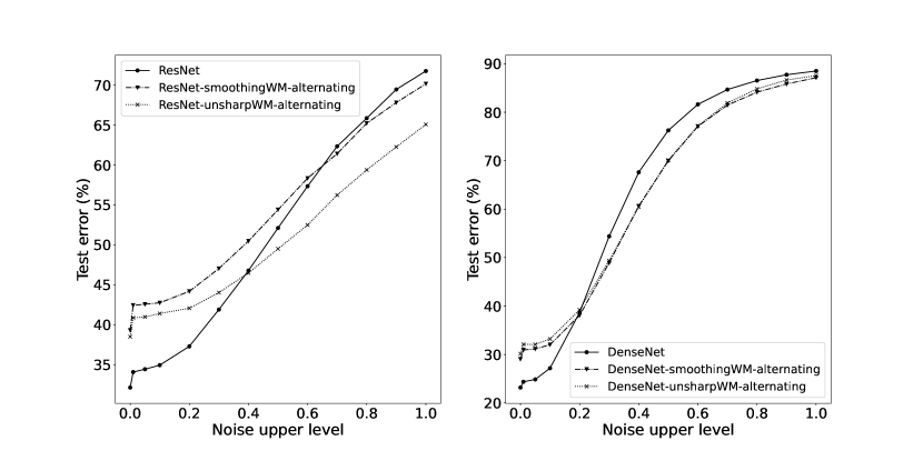
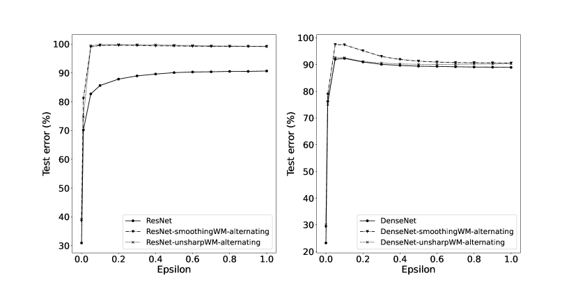
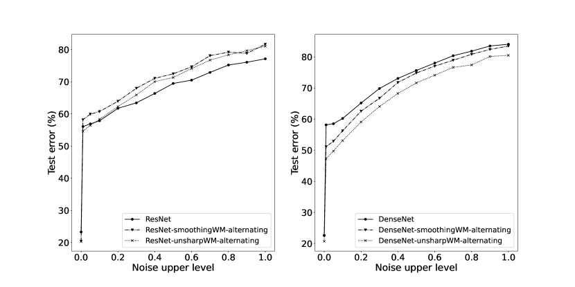
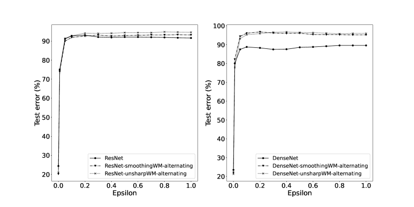
Robustness to noise results are shown in fig. 2, fig. 3 and fig. 4. For uniform noise, all of the WM variants tested on MNIST had better performance than the baseline, except for the non-alternating smoothing WM variant of ResNet. On CIFAR10, the alternating unsharp WM variant of ResNet showed lower performance than the baseline at lower noise, however, it becomes more robust than the baseline as the noise magnitude increases. All the alternating WM variants of DenseNet showed a similar behaviour. The alternating smoothing WM variants of ResNet, however, had less robustness at all noise levels. On iWildCam2019, all of the WM variants of ResNet were less robust than the baseline, while all the WM variants of DenseNet were more robust than the baseline.
Regarding adversarial noise results on MNIST, the unsharp WM variant of CNN was more robust than the baseline, while the baseline and all the other WM variants of CNN had similar performance. For ResNet, all the WM variants had either less or the same robustness compared to the baseline. All the WM variants of DenseNet were better than the baseline, except the alternating unsharp WM model which had similar performance to the baseline. On CIFAR10, both the baselines and the WM models of ResNet performed poorly, however, on average baseline was better than WM variants of ResNet, while WM variants of DenseNet were better on average than their baseline. iWildCam2019 had similar results to CIFAR10, where all the models, including the baseline, performed poorly. All ResNet models on iWildCam2019 had similar performance, while for DenseNet models, the baseline was on average better than the WM variants.
5 Discussion
We have benchmarked two reduction operations in WM layers: smoothing and unsharp. The smoothing operation is effectively a moving average over a window equal to the kernel area. Since this will introduce blurriness into the input which will accumulate further on stacking multiple layers, we benchmarked against another reduction operation that mimics the action of an unsharp filter to reduce the accumulating blurring effect. To further reduce the introduced distortion, we benchmarked models which alternate between having a normal convolutional layer and a WM layer.
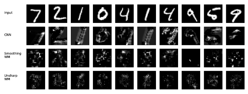
For the preliminary experiments based on CNN, the WM variant (no batchnorm and kernel size of 3) has a better performance than the corresponding vanilla CNN having the same number of FLOPS. We attribute this to two main factors. First, the higher capacity of the WM variant, due to its larger number of parameters, makes it more expressive. WM representation doesn’t, however, need to be in the same space as the CNN variant. The Grad-CAM (Selvaraju et al., 2016) visualization of both vanilla CNN and the two WM variants fig. 5 shows a substantial difference. While the CNN CAM is a blurry, diffused distortion of the input and sometimes activating for a large proportion of the background, the WM CAM is sharper, sparser and more localized with almost no diffused background activation, specially for the unsharp WM variant. We attribute this background activation sparsity to the feature selection ability of WM. Much like the way attentional techniques (Bahdanau et al., 2014; Vinyals et al., 2014; Xu et al., 2015; Hermann et al., 2015) can draw the network to focus on a subset of features, WM includes an elementwise multiplication by a weight map, that can in principle achieve feature selection on a pixel by pixel basis. On the other hand, normal convolution can’t achieve a similar effect because of weight sharing. The second possible reason for better performance consists of the scaling properties of the WM layer. This can in principle act like the normalization done by batchnorm layers. However, applying batchnorm can boost the performance of both CNN and WM variants, which indicates that the two approaches have an orthogonal component between them. Moreover, as we discuss below, batchnorm alone doesn’t protect against uniform noise and adversarial attacks. If we fix the number of parameters, instead of FLOPS, along with depth, we observe a clear advantage for WM variants. The WM variant with the same number of parameters and depth is better in performance by a large margin, and cheaper in FLOPS by around 100x. We attribute this to the large width compared to depth of the CNN variant, which makes it harder to optimize. On the other hand, WM can pack larger degrees of freedom without growing in width.
Increasing the kernel size enhances the performance of the CNN variant, while it lowers the performance of the WM variant. The enhanced CNN performance is due to increased capacity and a larger context made available by the larger receptive field. In the case of WM, the increased kernel size results in over smoothing and larger overlapping between adjacent receptive fields, effectively sharing more parameters and limiting the model’s effective capacity.
For deeper networks like ResNet and DenseNet, we will focus the discussion on the alternating models. The unsharp models show a similar or better test performance compared to the smoothing models across all datasets. This supports our motivation for introducing the unsharp operation to reduce distortion.
For uniform noise, we find that for all the WM models in MNIST and CIFAR10, at least one of the WM variants have better noise robustness than the baseline. In this subset, all of the WM models of CNN and DenseNet in MNIST have better noise robustness than the baseline. For uniform noise in iWildCam2019, the WM variants of DenseNet are more robust than the baseline, while the WM variants of ResNet are less robust than the baseline. For adversarial attacks, the WM variants of CNN and DenseNet have at least one model which is better than the baseline. For ResNet on MNIST, WM variants have the same as or less robustness than the baseline. For CIFAR10 and iWildCam2019, all the models are very sensitive to the adversarial noise, with mixed relative results between the WM variants and the baseline.
The above summary of results shows that the WM layer is very effective against random noise, while it doesn’t have the same efficacy against adversarial attacks. This may be explained by our hypothesis on the mechanism of the WM layer. The elementwise multiplication of the weight map by the input pixels, or any intermediate activation in general, can be considered as a feature selection mechanism. This implies that pixels that have large contribution to the accuracy will have large magnitude. The variance of any activation after applying the elementwise multiplication is then
| (5) |
where is the activation at the index , is the variance of that activation over the dataset, is the weight corresponding to the activation and is the elementwise multiplication operator.
We attribute the noise resistance introduced by the WM layer to the described amplification of the activation variance. This amplification is proportional to the weight magnitude and, hence, to the importance of the corresponding feature to the model performance. The amplification of variance increases the variations that the network encounters for the corresponding pixel/activation, which can be considered as an implicit augmentation of the dataset. This hypothesis, in turn, explains why it is performing better on random noise than adversarial attacks. While random noise has arbitrary direction, an adversarial attack can exploit gradient information to account for any differentiable component.
6 Conclusion
We introduced the weight map layer with its two variants as a generic architectural modification that can increase the robustness of convolutional neural networks to noise and adversarial attacks. We showed that it can be used to boost performance and increase noise robustness in small convolutional networks. Moreover, we showed that WM layers can be integrated into scaled up networks, ResNet and DenseNet, to increase their noise and adversarial attack robustness, while achieving comparable accuracy. We explained that the adaptive activation-variance amplification exhibited by the WM layer can explain its noise and adversarial attack robustness and the associated experimental observations regarding its dynamics. Future work has multiple promising directions with regards to finding more effective ways to integrate with more architectures to achieve noise robustness with more accuracy, providing more insights and experimental results regarding the dynamics of the WM layer and exploiting this further to enhance the accuracy and noise robustness of neural networks in general.
7 Acknowledgement
This work was partially supported by a grant from Microsoft’s AI for Earth program.
References
- Bahdanau et al. [2014] Dzmitry Bahdanau, Kyunghyun Cho, and Yoshua Bengio. Neural Machine Translation by Jointly Learning to Align and Translate. sep 2014. URL http://arxiv.org/abs/1409.0473.
- Chakraborty et al. [2018] Anirban Chakraborty, Manaar Alam, Vishal Dey, Anupam Chattopadhyay, and Debdeep Mukhopadhyay. Adversarial Attacks and Defences: A Survey. sep 2018. URL http://arxiv.org/abs/1810.00069.
- Fukushima and Miyake [1980] Kunihiko Fukushima and Sei Miyake. Neocognitron: Self-organizing network capable of position-invariant recognition of patterns. In Proc. 5th Int. Conf. Pattern Recognition, volume 1, pages 459–461, 1980.
- Ganin et al. [2015] Yaroslav Ganin, Evgeniya Ustinova, Hana Ajakan, Pascal Germain, Hugo Larochelle, François Laviolette, Mario Marchand, and Victor Lempitsky. Domain-Adversarial Training of Neural Networks. may 2015. URL https://arxiv.org/abs/1505.07818.
- Gao et al. [2017] Ji Gao, Beilun Wang, Zeming Lin, Weilin Xu, and Yanjun Qi. DeepCloak: Masking Deep Neural Network Models for Robustness Against Adversarial Samples. feb 2017. URL http://arxiv.org/abs/1702.06763.
- Ghosh et al. [2018] Partha Ghosh, Arpan Losalka, and Michael J Black. Resisting Adversarial Attacks using Gaussian Mixture Variational Autoencoders. may 2018. URL http://arxiv.org/abs/1806.00081.
- Gonzalez et al. [2002] Rafael C Gonzalez, Richard E Woods, and Others. Digital image processing [M]. Publishing house of electronics industry, 141(7):184–186, 2002.
- Goodfellow et al. [2014] Ian J. Goodfellow, Jonathon Shlens, and Christian Szegedy. Explaining and Harnessing Adversarial Examples. dec 2014. URL http://arxiv.org/abs/1412.6572.
- Ha et al. [2016] David Ha, Andrew Dai, and Quoc V. Le. HyperNetworks. sep 2016. URL http://arxiv.org/abs/1609.09106.
- He et al. [2015] Kaiming He, Xiangyu Zhang, Shaoqing Ren, and Jian Sun. Deep Residual Learning for Image Recognition. dec 2015. URL http://arxiv.org/abs/1512.03385.
- Hermann et al. [2015] Karl Moritz Hermann, Tomáš Kočiský, Edward Grefenstette, Lasse Espeholt, Will Kay, Mustafa Suleyman, and Phil Blunsom. Teaching Machines to Read and Comprehend. jun 2015. URL http://arxiv.org/abs/1506.03340.
- Hinton et al. [2015] Geoffrey Hinton, Oriol Vinyals, and Jeff Dean. Distilling the Knowledge in a Neural Network. mar 2015. URL http://arxiv.org/abs/1503.02531.
- Hosseini et al. [2017] Hossein Hosseini, Yize Chen, Sreeram Kannan, Baosen Zhang, and Radha Poovendran. Blocking Transferability of Adversarial Examples in Black-Box Learning Systems. mar 2017. URL https://arxiv.org/abs/1703.04318.
- Huang et al. [2016] Gao Huang, Zhuang Liu, Laurens van der Maaten, and Kilian Q. Weinberger. Densely Connected Convolutional Networks. aug 2016. URL http://arxiv.org/abs/1608.06993.
- Ioffe and Szegedy [2015] Sergey Ioffe and Christian Szegedy. Batch Normalization: Accelerating Deep Network Training by Reducing Internal Covariate Shift. feb 2015. URL http://arxiv.org/abs/1502.03167.
- Jin et al. [2015] Jonghoon Jin, Aysegul Dundar, and Eugenio Culurciello. Robust Convolutional Neural Networks under Adversarial Noise. nov 2015. URL http://arxiv.org/abs/1511.06306.
- Krizhevsky et al. [2012] Alex Krizhevsky, Ilya Sutskever, and Geoffrey E. Hinton. ImageNet Classification with Deep Convolutional Neural Networks, 2012. URL http://papers.nips.cc/paper/4824-imagenet-classification-with-deep-convolutional-neural-networ.
- Lamb et al. [2018] Alex Lamb, Jonathan Binas, Anirudh Goyal, Dmitriy Serdyuk, Sandeep Subramanian, Ioannis Mitliagkas, and Yoshua Bengio. Fortified Networks: Improving the Robustness of Deep Networks by Modeling the Manifold of Hidden Representations. apr 2018. URL http://arxiv.org/abs/1804.02485.
- LeCun et al. [1989] Y. LeCun, B. Boser, J. S. Denker, D. Henderson, R. E. Howard, W. Hubbard, and L. D. Jackel. Backpropagation Applied to Handwritten Zip Code Recognition. Neural Computation, 1(4):541–551, dec 1989. ISSN 0899-7667. doi: 10.1162/neco.1989.1.4.541. URL http://www.mitpressjournals.org/doi/10.1162/neco.1989.1.4.541.
- Lyu et al. [2015] Chunchuan Lyu, Kaizhu Huang, and Hai-Ning Liang. A Unified Gradient Regularization Family for Adversarial Examples. In 2015 IEEE International Conference on Data Mining, pages 301–309. IEEE, nov 2015. ISBN 978-1-4673-9504-5. doi: 10.1109/ICDM.2015.84. URL http://ieeexplore.ieee.org/document/7373334/.
- Papernot and McDaniel [2017] Nicolas Papernot and Patrick McDaniel. Extending Defensive Distillation. may 2017. URL http://arxiv.org/abs/1705.05264.
- Papernot et al. [2016a] Nicolas Papernot, Patrick McDaniel, and Ian Goodfellow. Transferability in Machine Learning: from Phenomena to Black-Box Attacks using Adversarial Samples. may 2016a. URL http://arxiv.org/abs/1605.07277.
- Papernot et al. [2016b] Nicolas Papernot, Patrick McDaniel, Xi Wu, Somesh Jha, and Ananthram Swami. Distillation as a Defense to Adversarial Perturbations Against Deep Neural Networks. In 2016 IEEE Symposium on Security and Privacy (SP), pages 582–597. IEEE, may 2016b. ISBN 978-1-5090-0824-7. doi: 10.1109/SP.2016.41. URL http://ieeexplore.ieee.org/document/7546524/.
- Pontes-Filho and Liwicki [2018] Sidney Pontes-Filho and Marcus Liwicki. Bidirectional Learning for Robust Neural Networks. may 2018. URL http://arxiv.org/abs/1805.08006.
- Seltzer et al. [2013] Michael L. Seltzer, Dong Yu, and Yongqiang Wang. An investigation of deep neural networks for noise robust speech recognition. In 2013 IEEE International Conference on Acoustics, Speech and Signal Processing, pages 7398–7402. IEEE, may 2013. ISBN 978-1-4799-0356-6. doi: 10.1109/ICASSP.2013.6639100. URL http://ieeexplore.ieee.org/document/6639100/.
- Selvaraju et al. [2016] Ramprasaath R. Selvaraju, Michael Cogswell, Abhishek Das, Ramakrishna Vedantam, Devi Parikh, and Dhruv Batra. Grad-CAM: Visual Explanations from Deep Networks via Gradient-based Localization. oct 2016. URL http://arxiv.org/abs/1610.02391.
- Shaham et al. [2015] Uri Shaham, Yutaro Yamada, and Sahand Negahban. Understanding Adversarial Training: Increasing Local Stability of Neural Nets through Robust Optimization. nov 2015. doi: 10.1016/j.neucom.2018.04.027. URL http://arxiv.org/abs/1511.05432http://dx.doi.org/10.1016/j.neucom.2018.04.027.
- Sinha et al. [2018] Ayan Sinha, Zhao Chen, Vijay Badrinarayanan, and Andrew Rabinovich. Gradient Adversarial Training of Neural Networks. jun 2018. URL http://arxiv.org/abs/1806.08028.
- Sun et al. [2017] Zhun Sun, Mete Ozay, and Takayuki Okatani. HyperNetworks with statistical filtering for defending adversarial examples. nov 2017. URL http://arxiv.org/abs/1711.01791.
- Szegedy et al. [2013] Christian Szegedy, Wojciech Zaremba, Ilya Sutskever, Joan Bruna, Dumitru Erhan, Ian Goodfellow, and Rob Fergus. Intriguing properties of neural networks. dec 2013. URL https://arxiv.org/abs/1312.6199.
- Tramèr et al. [2017] Florian Tramèr, Alexey Kurakin, Nicolas Papernot, Ian Goodfellow, Dan Boneh, and Patrick McDaniel. Ensemble Adversarial Training: Attacks and Defenses. may 2017. URL http://arxiv.org/abs/1705.07204.
- Vinyals et al. [2014] Oriol Vinyals, Lukasz Kaiser, Terry Koo, Slav Petrov, Ilya Sutskever, and Geoffrey Hinton. Grammar as a Foreign Language. dec 2014. URL http://arxiv.org/abs/1412.7449.
- Xu et al. [2015] Kelvin Xu, Jimmy Ba, Ryan Kiros, Kyunghyun Cho, Aaron Courville, Ruslan Salakhutdinov, Richard Zemel, and Yoshua Bengio. Show, Attend and Tell: Neural Image Caption Generation with Visual Attention. feb 2015. URL http://arxiv.org/abs/1502.03044.
- Xu et al. [2017] Weilin Xu, David Evans, and Yanjun Qi. Feature Squeezing: Detecting Adversarial Examples in Deep Neural Networks. apr 2017. doi: 10.14722/ndss.2018.23198. URL http://arxiv.org/abs/1704.01155http://dx.doi.org/10.14722/ndss.2018.23198.