\sectiondot

subsection \sectiondotsubsubsection

Contact-Aided Invariant Extended Kalman Filtering for
Robot State Estimationthanks: Submitted for journal publication. rosshart@umich.edu

Ross Hartley Robotics Institute and College of Engineering, University of Michigan, Ann Arbor, MI, USA.    Maani Ghaffari22footnotemark: 2    Ryan M. Eustice22footnotemark: 2    Jessy W. Grizzle22footnotemark: 2
Abstract

Legged robots require knowledge of pose and velocity in order to maintain stability and execute walking paths. Current solutions either rely on vision data, which is susceptible to environmental and lighting conditions, or fusion of kinematic and contact data with measurements from an inertial measurement unit (IMU). In this work, we develop a contact-aided invariant extended Kalman filter (InEKF) using the theory of Lie groups and invariant observer design. This filter combines contact-inertial dynamics with forward kinematic corrections to estimate pose and velocity along with all current contact points. We show that the error dynamics follows a log-linear autonomous differential equation with several important consequences: (a) the observable state variables can be rendered convergent with a domain of attraction that is independent of the system’s trajectory; (b) unlike the standard EKF, neither the linearized error dynamics nor the linearized observation model depend on the current state estimate, which (c) leads to improved convergence properties and (d) a local observability matrix that is consistent with the underlying nonlinear system. Furthermore, we demonstrate how to include IMU biases, add/remove contacts, and formulate both world-centric and robo-centric versions. We compare the convergence of the proposed InEKF with the commonly used quaternion-based EKF though both simulations and experiments on a Cassie-series bipedal robot. Filter accuracy is analyzed using motion capture, while a LiDAR mapping experiment provides a practical use case. Overall, the developed contact-aided InEKF provides better performance in comparison with the quaternion-based EKF as a result of exploiting symmetries present in system.

1 Introduction

Legged robots have the potential to transform the logistics and package delivery industries, become assistants in our homes, and aide in search and rescue [29]. In order to develop motion planning algorithms and robust feedback controllers for these tasks, accurate estimates of the robot’s state are needed. Some states, such as joint angles, can be directly measured using encoders, while other states, such as the robot’s pose and velocity, require additional sensors. Most legged robots are equipped with an inertial measurement unit (IMU) that can measure linear acceleration and angular velocity, albeit with noise and bias perturbations. Consequently, nonlinear observers are typically used to fuse leg odometry and inertial measurements to infer trajectory, velocity, and calibration parameters [68, 14, 35, 53]. In view of a practical solution, designing a globally convergent observer is sacrificed for one with at best local properties, such as the extended Kalman filter (EKF[42, 52, 79, 75]. This EKF-based approach is computationally efficient and easily customizable, allowing successful implementation on a number of legged robots with rigorous real-time performance requirements [15, 17, 36, 65].

Accurate pose estimation can be combined with visual data to build maps of the environment [37]. Then such maps can be used in gait selection to improve the stability of a robot while walking on uneven terrains and as a basis for high-level motion planning. Although there have been many recent advancements in visual-inertial-odometry and simultaneous localization and mapping (SLAM) [66, 48, 38], these algorithms often rely on visual data for pose estimation. This means that the observer (and ultimately the feedback controller) can be adversely affected by rapid changes in lighting as well as the operating environment. It is therefore beneficial to develop a low-level state estimator that fuses data only from proprioceptive sensors to form accurate high-frequency state estimates. This approach was taken by Bloesch et al. [15] when developing a quaternion-based extended Kalman filter (QEKF) that combines inertial, contact, and kinematic data to estimate the robot’s base pose, velocity, and a number of contact states. In this article, we expand upon these ideas to develop an invariant extended Kalman filter (InEKF) that has improved convergence and consistency properties allowing for a more robust observer that is suitable for long-term autonomy.

The theory of invariant observer design is based on the estimation error being invariant under the action of a matrix Lie group [1, 20], which has recently led to the development of the InEKF111We use the InEKF acronym to distinguish from an iterated-EKF (IEKF). [18, 8, 10, 11] with successful applications and promising results in simultaneous localization and mapping [8, 86] and aided inertial navigation systems [4, 5, 8, 83]. The invariance of the estimation error with respect to a Lie group action is referred to as a symmetry of the system [5]. Summarized briefly, Barrau and Bonnabel [10] showed that if the state is defined on a Lie group, and the dynamics satisfy a particular “group affine” property, then the symmetry leads to the estimation error satisfying a “log-linear” autonomous differential equation on the Lie algebra. In the deterministic case, this linear system can be used to exactly recover the estimated state of the nonlinear system as it evolves on the group. The log-linear property therefore allows the design of a nonlinear observer or state estimator with strong convergence properties.

1.1 Contribution

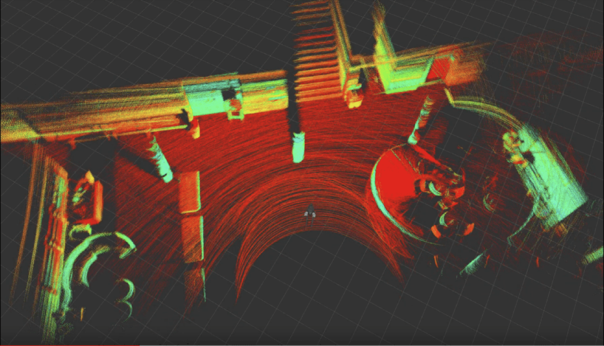
In this article, we derive an InEKF for a system containing IMU and contact sensor dynamics, with forward kinematic correction measurements. We show that the defined deterministic system satisfies the “group affine” property, and therefore, the error dynamics is exactly log-linear. In practice, with the addition of sensor noise and IMU bias, this log-linear error system is only approximate; we show, however, that in many cases the proposed InEKF is still preferred over standard QEKFs due to superior convergence and consistency properties. We demonstrate the utility and accuracy of the developed observer through a series of LiDAR mapping experiments performed on a Cassie-series biped robot.

In summary, this work makes the following contributions:

  1. 1.

    Derivation of a continuous-time right-invariant EKF for an IMU/contact process model with a forward kinematic measurement model; the observability analysis is also presented;

  2. 2.

    State augmentation with IMU biases;

  3. 3.

    Evaluations of the derived observer in simulation and hardware experiments using a 3D bipedal robot;

  4. 4.

    Alternative derivation of the observer using a left-invariant error definition;

  5. 5.

    Detailed explanation of the connection between the invariant error choice and the world-centric and robo-centric estimator formulations;

  6. 6.

    Equations provided for analytical discretization of the proposed observers; and

  7. 7.

    Development of an open-source C++ library for aided-inertial navigation using the InEKF https://github.com/RossHartley/invariant-ekf.

1.2 Outline

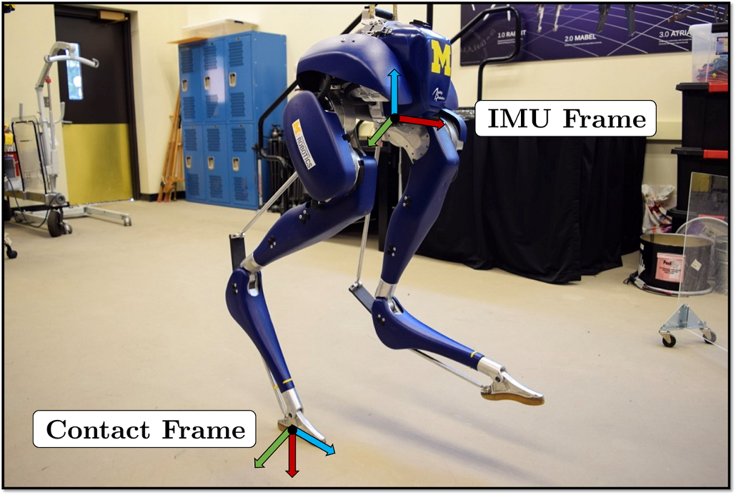
The remainder of this article is organized as follows. Background and related work are given in section 2. Section 3 provides the necessary preliminary material needed for understanding the InEKF formulation, which is motived by an example from attitude dynamics in section 4. Section 5 provides the derivation of a right-invariant extended Kalman filter (RIEKF) for contact-inertial navigation with a right-invariant forward kinematic measurement model. In Section 6, we present simulation results comparing the convergence properties to a state-of-the-art QEKF. Section 7 discusses the state augmentation of the previously derived InEKF with IMU bias. The consequences of adding and removing of contact points in the estimator are described in Section 8. Experimental evaluations on a 3D biped robot, shown in Figure 1, are presented in Section 9 along with an application towards LiDAR-based terrain mapping. Section 10 provides an alternative derivation of the proposed observer using the left-invariant dynamics along with an explanation of how to easily switch between the two formulations. Section 11 details how these equations can be modified to create a “robot-centric” estimator. Section 12 itemizes additional sensor measurements that fit within the InEKF framework and describes the relation between the developed filter and landmark-based SLAM. Finally, Section 13 concludes the article and suggests future directions. Details about time-discretization and useful Lie group expressions are given in the appendix.
Refer to caption
Figure 1: A Cassie-series biped robot is used for both simulation and experimental results. The robot was developed by Agility Robotics and has 20 degrees of freedom, 10 actuators, joint encoders, and an inertial measurement unit (IMU). The contact and IMU frames used in this work are depicted above.

2 Background and Related work

In this section, we first review the Kalman filtering literature to locate the proposed state estimator within the relate work. Then, we review the state estimation techniques for humanoid and legged robots.

2.1 Kalman Filtering

Filtering methods involve estimating the robot’s current state (and potentially landmarks) using the set of all measurements up to the current time [2, 41, 73]. When the process model and measurements are linear, and the noise is white and Gaussian, Kalman filtering [51] provides an optimal method (minimum mean squared error) for state estimation. The general process for Kalman filtering involves two phases, propagation and correction. The state is typically represented using a Gaussian random vector, which is parameterized by a mean and a covariance. During the propagation phase, the previous state and covariance estimate are propagated forward in time using the system dynamics (alternatively known as the process model). When a measurement is obtained, the state and covariance estimate are corrected using the measurement model along with an associated measurement noise covariance.

Although the Kalman filter provides a method for optimal linear filtering, most practical mobile robots have nonlinear system dynamics, and many useful sensor models are also nonlinear. For these cases, an EKF can be designed, which utilizes Taylor series expansions to linearize the process and measurement models around the current state estimate [77]. Due to its low computational complexity and accurate performance, the EKF quickly became the de facto standard of nonlinear filtering for many mobile robot applications, including wheeled vehicles, drones, and legged robots [24, 70, 15]. The EKFs has also been proposed to solve the SLAM problem [74]. However, since the nonlinear system is linearized about the current state estimate, the EKF is, at best, only a locally stable observer [76, 52]. The local convergence proofs are based on Lipschitz bounds of the nonlinear terms in a model, and hence “the more nonlinear a system is, the worse an EKF may perform”. Importantly, if the state estimate is initialized poorly, it is possible for the filter to diverge. In addition, because an EKFs uses a systems linearization about the current estimate, states that are unobservable can spuriously be treated as observable by the filter. While, this can be mitigated through the use of an observability-constrained EKF developed by Huang et al. [49], it cannot be altogether avoided.

For many systems, the error-state (or indirect) EKF offers superior performance to the standard (total state or direct) form. As the name implies, the error-state extended Kalman filter (ErEKF) is formulated using the errors, such as pose and velocity errors, as the filter variables, while the standard EKF tracks the states themselves (pose and velocity directly) [59, 69, 79, 75]. Under small noise assumptions, this leads to linear error dynamics which are then used for covariance propagation in the error-state filter. The measurement model is also rewritten with respect to these errors. Although the error dynamics are linear in the error variables, they may still depend on the current state estimate, which if initialized poorly, will degrade the performance of the filter. However, the approximately linear nature of the error dynamics may respect the linear assumptions of the original Kalman filter better than the underlying system dynamics, which can lead to improved performance [59].

Perhaps the most important feature of the ErEKF is the ability to circumvent dynamic modeling [69]. This is done by replacing the potentially complicated process model with a relatively simple IMU integration model (also known as strapdown modeling) [78, 62, 82]. Essentially, the IMU’s angular velocity and linear acceleration measurements are integrated to propagate the state estimate, while the covariance is propagated using the error dynamics. Additional (independent) sensor measurements will correct the estimated error, which can then be used to update the state estimate. Using this method, there is no longer a need to formulate complicated, platform-specific dynamics models, which may require a large number of state variables and is likely to be exceedingly nonlinear. The “strapdown” ErEKFs has proven to yield highly accurate results (even with a low-cost IMUs) and continues to form the basis of many inertial navigation systems [13, 54, 79, 75, 15].

In the standard formulation of Kalman filtering theory, the system evolves on Euclidean spaces. However, in many cases, the state variables we are interested in lie on a manifold. For example, the orientation of a 3D rigid body is represented by an element of the special orthogonal group, SO(3)SO3\mathrm{SO}(3). This matrix Lie group is defined by the set of orthogonal 3×3333\times 3 matrices with a determinant of one. While the matrix contains nine variables, yet the dimension of the manifold is only three. One common approach is to parameterize SO(3)SO3\mathrm{SO}(3) using local coordinates such as three Euler or Tait-Bryan angles [39, 71]. This allows the standard ErEKF equations to be applied; however, these local parameterizations are often arbitrary (and therefore confusing) and contain singularities (the well-known Gimbal lock problem). Alternatively, it is possible to represent 3D orientation using quaternions, which are a four-dimensional double cover (a two to one diffeomorphism) of SO(3)SO3\mathrm{SO}(3). Using quaternions eliminates the singularities; however, modifications to the standard ErEKF equations have to be made [75, 79]. In brief, while the orientation is represented by a four-dimensional quaternion, the orientation error has to be defined by a 3limit-from33-vector (in the Lie algebra of SO(3)SO3\mathrm{SO}(3)) and the associated covariance by a 3×3333\times 3 matrix in order to prevent degeneracy. Also, the orientation corrections are done through quaternion multiplication instead of vector addition. This QEKF 222The quaternion-based formulation of EKFs is also sometimes called “multiplicative filtering” (MEKF) due to the orientation correction being done through quaternion multiplication [60]. has been well studied and implemented on a number of platforms, ranging from spacecraft [63, 54] to legged robots [15, 68, 36].

It turns out, many useful robot states can be characterized using matrix Lie groups. Examples include 2D orientation, SO(2)SO2\mathrm{SO}(2), 3D orientation, SO(3)SO3\mathrm{SO}(3), and 3D pose (orientation and position), SE(3)SE3\mathrm{SE}(3). If the state to be estimated is a matrix Lie group, it is possible to further improve the EKF filtering approach. Bourmaud et al. [22, 23] developed versions of both discrete and continuous-time EKFs for systems where the state dynamics and measurements evolve on matrix Lie groups. In these formulations, noise is represented as a concentrated Gaussian on Lie groups [80, 81], which is a generalization of the multivariate Gaussian distribution. In essence, noise is represented as a Gaussian in the tangent space about a point on the manifold. This noise is then mapped to the Lie group through the use of the group’s exponential map, resulting in a decidedly non-Gaussian distribution on the manifold. An improved state estimate is obtained due to the filter taking into account the geometry and structure of the problem [23].

Most recently, a new type of EKF has been developed that is rooted in the theory of invariant observer design, in which the estimation error is invariant under the action of a Lie group [1, 20]. This invariance is referred to as the symmetries of the system [5]. This work led to the development of the InEKF [18, 8, 10, 11], with successful applications and promising results in SLAM [8, 86] and aided INSs [21, 4, 5, 8, 83]. Similar to the above mentioned EKFs on matrix Lie groups, the state is again represented as a matrix Lie group and the noise as a concentrated Gaussian on the group.

However, the InEKF exploits available system symmetries to further improve filtering results. The culminating result of the InEKF states that if a system satisfies a “group-affine” property, the estimation error satisfies a “log-linear” autonomous differential equation on the Lie algebra of the corresponding Lie group [11, 8]. In other words, the system linearization does not depend upon the estimated states. Therefore, one can design a nonlinear state estimator with strong convergence properties. Surprisingly, many mobile robot state estimation problems can be solved within the InEKF framework. This includes attitude estimation [18], inertial odometry [11, 8], velocity-aided inertial navigation [21], landmark-aided navigation [8], GPS and magnetometer-aided navigation [4], and even EKF-based SLAM. In this article, we extend this class of solutions to contact-aided inertial navigation [46], where forward kinematics is used to correct an inertial and contact-based process model. This approach successfully allows an InEKF to be used for legged robot state estimation.

2.2 Legged Robot and Humanoid State Estimation

Legged robots are a subclass of mobile robots that locomote through direct and switching contact with the environment. These robots typically contain proprioceptive sensors, such as IMU, joint encoders, and contact sensors. In addition, some legged robots, especially humanoids, also have access to exteroceptive sensors, namely cameras and LiDARs. As with all mobile robots, state estimation for legged robots is critical for mapping, planning, designing feedback controllers, and developing general autonomy. In this section, an overview of notable techniques for legged robot state estimation is given.

The simplest approach for estimation of a legged robot’s spatial location and velocity is kinematic dead-reckoning, otherwise known as kinematic odometry. This involves estimating relative transformations using only kinematic and contact measurements. In particular, encoder measurements and the kinematics model are used to track the position, orientation, and velocity of the robot’s base frame based on the assumption that a stance foot remains fixed to the ground. Although this method can be easily implemented, the state estimate is typically noisy due to kinematic modeling errors, encoder noise, and foot slip [67]. When only one foot is in contact with the ground, this “static contact assumption” may be violated. For example, if the robot has point feet, the stance foot position may remain fixed, but the foot orientation is free to rotate (without changing the joint angles). Therefore, a gyroscope is often used to provide angular velocity measurements which allows the robot’s body velocity to be recovered.

Alternatively, if the terrain is known a priori and at least three noncollinear point feet are on the ground, Lin et al. [55] showed that the robot’s instantaneous base pose can be computed through kinematics. These kinematic-based methods have been implemented on a number of legged robots including a planar one-legged hopper [47], the CMU Ambler hexapod [67], the RHex hexapod [55], and the biped robot MARLO [31, 32]. However, due to the high amounts of noise coming from encoders and foot slip, the velocity estimate typically needs to be heavily filtered before becoming usable in the feedback controller [44]. In addition, this noise causes the position and orientation estimates to drift substantially rendering the estimator impractical for mapping and autonomy tasks.

Fortunately, legged robots are often equipped with additional sensors such as IMUs, GPS, cameras, or LiDARs which provide independent, noisy odometry measurements. Much of the literature on legged robot state estimation focuses on fusing these measurements (potentially with kinematic odometry) using filtering and smoothing methods. Singh et al. [72] combined inertial measurements with optical flow measurements in a four-phase hybrid EKF. This required explicit dynamic modeling of the robot in flight, landing, stance, and thrust phases. Lin et al. [56] took a similar model-based approach and used an EKF to fuse kinematic information with IMU measurements to estimate the state of a hexapod. Cobano et al. [30] developed an EKF that fuses kinematic odometry and magnetometer readings with position measurements from a GPS to localize a SILO4 quadruped outdoors. This implementation fixes the issues with unbounded drift, but cannot operate in GPS-denied environments. If a prior terrain map is known, Chitta et al. [28] showed that it is possible to solve the localization problem for legged robots using only proprioceptive sensors and a particle filter. The key idea was that if the robot “senses” that a terrain change through kinematics, then this limits the potential locations the robot can be in a known map. The method was demonstrated on the LittleDog quadruped.

A breakthrough came in 2012 when Bloesch et al. [15] combined inertial and kinematic measurements in an observability-constrained ErEKF using the strapdown IMU modeling approach. In this work, no a priori knowledge of the terrain is assumed, and the IMU integration model completely eliminates the need for dynamic modeling of the robot. Therefore, the derived filter equations are general enough to be used on any legged robot. The key idea was to augment the state vector with the set of all foot positions currently in contact with the environment. During the prediction phase, the foot contact dynamics are assumed to be Brownian motion, which can account for some foot slippage. In the correction phase, forward-kinematic position measurements are used to correct the estimated state. This work was conducted on the StarlETH quadruped robot. If the stance feet orientations also remain constant, as is the case for many humanoids, Rotella et al. [68] showed that this ErEKF can be extended to allow forward-kinematic orientation measurements. The same group also formulated a similar unscented Kalman filter that uses forward-kinematic velocity measurements to correct inertial predictions and to accurately detect foot slip [16]. A detailed analysis of these filtering techniques combined with methods for incorporating computer vision can be found in Bloesch [17]. Due to the complexity involved in accurately formulating dynamic models, many groups have since adopted this IMU motion model approach to legged robot state estimation [84, 36, 46].

This combined inertial and kinematic filtering approach yields an estimate of the robot’s base pose and velocity. However, some legged robots require additional states to be estimated. Hwangbo et al. [50] formulated a probabilistic contact estimator for cases when contact sensors are unavailable. Xinjilefu et al. [84] developed a decoupled EKF that is able to estimate the full state of the humanoid robot ATLAS, including base states, joint angles, and joint velocities. Using proprioceptive sensing only, Bloesch et al. [15] proved that the absolute positions and yaw angles are unobservable. Thus, over time, estimates of these quantities will drift unboundedly. This is unacceptable for global mapping and planning algorithms; however, local elevation maps can still be obtained [37]. Fallon et al. [36] proposed a method for drift-free state estimation for the humanoid ATLAS. In their implementation, inertial and kinematic measurements were fused to yield accurate odometry. Point cloud data from a LiDAR sensor was used with a particle filter to localize the robot into a pre-built map. This approach provided corrections of position and yaw to obtain a drift-free estimate of the state. Nobili et al. [64] took a similar approach but used the Iterative Closest Point (ICP) algorithm to perform LiDAR-based point cloud matching. The algorithm was tested on the HyQ quadruped robot.

In this article, we propose using an InEKF to estimate the base pose and velocity of a general legged robot. The approach we take is most similar to Bloesch et al. [15], however we model the entire state as a single matrix Lie group as opposed to a decoupled state approach. This allows us to take advantage of the geometry and symmetry of the estimation problem to formulate autonomous error dynamics. In addition with our formulation, the linearizations are independent of the state estimate resulting in improved convergence properties, especially for poor state initializations. We formulate both world-centric and robo-centric state estimators highlighting the relation between the left- and right-invariant error dynamics. In addition, we provide exact analytical time-discretizations of both filters. The implemented filters can be run at high speeds (>2000Hzabsent2000Hz>2000\mathop{\mathrm{Hz}}) and can be directly used for accurate local odometry. We demonstrate this idea through a LiDAR terrain mapping application on a Cassie-series biped robot.

3 Theoretical background and preliminaries

We assume a matrix Lie group [43, 27] denoted 𝒢𝒢\mathcal{G} and its associated Lie Algebra denoted 𝔤𝔤\mathfrak{g}. If elements of 𝒢𝒢\mathcal{G} are n×n𝑛𝑛n\times n matrices, then so are elements of 𝔤𝔤\mathfrak{g}. When doing calculations, it is very convenient to let

():dim𝔤𝔤:superscriptsuperscriptdim𝔤𝔤{(\cdot)}^{\wedge}:\mathbb{R}^{\mathrm{dim}\mathfrak{g}}\to\mathfrak{g}

be the linear map that takes elements of the tangent space of 𝒢𝒢\mathcal{G} at the identity to the corresponding matrix representation so that the exponential map of the Lie group, exp:dim𝔤𝒢:superscriptdim𝔤𝒢\exp:\mathbb{R}^{\mathrm{dim}\mathfrak{g}}\to\mathcal{G}, is computed by

exp(𝝃)=expm(𝝃),𝝃subscript𝑚superscript𝝃\exp(\boldsymbol{\xi})=\exp_{m}({\boldsymbol{\xi}}^{\wedge}),

where expm()subscript𝑚\exp_{m}(\cdot) is the usual exponential of n×n𝑛𝑛n\times n matrices.

A process dynamics evolving on the Lie group with state at time t𝑡t, Xt𝒢subscriptX𝑡𝒢\textbf{X}_{t}\in\mathcal{G}, is denoted by

ddtXt=fut(Xt),dd𝑡subscriptX𝑡subscript𝑓subscript𝑢𝑡subscriptX𝑡\dfrac{\mathrm{d}}{\mathrm{d}t}\textbf{X}_{t}=f_{u_{t}}(\textbf{X}_{t}),

and X¯tsubscript¯X𝑡\bar{\textbf{X}}_{t} is used to denote an estimate of the state. The state estimation error is defined using right or left multiplication of Xt1superscriptsubscriptX𝑡1\textbf{X}_{t}^{-1} as follows.

Definition 1 (Left and Right Invariant Error).

The right- and left-invariant errors between two trajectories XtsubscriptX𝑡\textbf{X}_{t} and X¯tsubscript¯X𝑡\bar{\textbf{X}}_{t} are:

𝜼tr=X¯tXt1=(X¯tL)(XtL)1(Right-Invariant)𝜼tl=Xt1X¯t=(LX¯t)1(LXt),(Left-Invariant)\begin{split}\boldsymbol{\eta}_{t}^{r}&=\bar{\textbf{X}}_{t}\textbf{X}_{t}^{-1}=(\bar{\textbf{X}}_{t}\textbf{L})(\textbf{X}_{t}\textbf{L})^{-1}\quad\text{(Right-Invariant)}\\ \boldsymbol{\eta}_{t}^{l}&=\textbf{X}_{t}^{-1}\bar{\textbf{X}}_{t}=(\textbf{L}\bar{\textbf{X}}_{t})^{-1}(\textbf{L}\textbf{X}_{t}),\quad\text{(Left-Invariant)}\end{split} (1)

where L is an arbitrary element of the group.

The following two theorems are the fundamental results for deriving an InEKF and show that by correct parametrization of the error variable, a wide range of nonlinear problems can lead to linear error equations.

Theorem 1 (Autonomous Error Dynamics [10]).

A system is group affine if the dynamics, fut()subscript𝑓subscript𝑢𝑡f_{u_{t}}(\cdot), satisfies:

fut(X1X2)=fut(X1)X2+X1fut(X2)X1fut(Id)X2subscript𝑓subscript𝑢𝑡subscriptX1subscriptX2subscript𝑓subscript𝑢𝑡subscriptX1subscriptX2subscriptX1subscript𝑓subscript𝑢𝑡subscriptX2subscriptX1subscript𝑓subscript𝑢𝑡subscriptI𝑑subscriptX2f_{u_{t}}(\textnormal{{X}}_{1}\textnormal{{X}}_{2})=f_{u_{t}}(\textnormal{{X}}_{1})\textnormal{{X}}_{2}+\textnormal{{X}}_{1}f_{u_{t}}(\textnormal{{X}}_{2})-\textnormal{{X}}_{1}f_{u_{t}}(\textbf{{I}}_{d})\textnormal{{X}}_{2} (2)

for all t>0𝑡0t>0 and X1,X2𝒢subscriptX1subscriptX2𝒢\textnormal{{X}}_{1},\textnormal{{X}}_{2}\in\mathcal{G}. Furthermore, if this condition is satisfied, the right- and left-invariant error dynamics are trajectory independent and satisfy:

ddt𝜼trdd𝑡superscriptsubscript𝜼𝑡𝑟\displaystyle\dfrac{\mathrm{d}}{\mathrm{d}t}\boldsymbol{\eta}_{t}^{r} =gut(𝜼tr)wheregut(𝜼r)absentsubscript𝑔subscript𝑢𝑡superscriptsubscript𝜼𝑡𝑟wheresubscript𝑔subscript𝑢𝑡superscript𝜼𝑟\displaystyle=g_{u_{t}}(\boldsymbol{\eta}_{t}^{r})\quad\text{where}\quad g_{u_{t}}(\boldsymbol{\eta}^{r}) =fut(𝜼r)𝜼rfut(Id)absentsubscript𝑓subscript𝑢𝑡superscript𝜼𝑟superscript𝜼𝑟subscript𝑓subscript𝑢𝑡subscriptI𝑑\displaystyle=f_{u_{t}}(\boldsymbol{\eta}^{r})-\boldsymbol{\eta}^{r}f_{u_{t}}(\textbf{{I}}_{d})
ddt𝜼tldd𝑡superscriptsubscript𝜼𝑡𝑙\displaystyle\dfrac{\mathrm{d}}{\mathrm{d}t}\boldsymbol{\eta}_{t}^{l} =gut(𝜼tl)wheregut(𝜼l)absentsubscript𝑔subscript𝑢𝑡superscriptsubscript𝜼𝑡𝑙wheresubscript𝑔subscript𝑢𝑡superscript𝜼𝑙\displaystyle=g_{u_{t}}(\boldsymbol{\eta}_{t}^{l})\quad\text{where}\quad g_{u_{t}}(\boldsymbol{\eta}^{l}) =fut(𝜼l)fut(Id)𝜼labsentsubscript𝑓subscript𝑢𝑡superscript𝜼𝑙subscript𝑓subscript𝑢𝑡subscriptI𝑑superscript𝜼𝑙\displaystyle=f_{u_{t}}(\boldsymbol{\eta}^{l})-f_{u_{t}}(\textbf{{I}}_{d})\boldsymbol{\eta}^{l}

In the above, Id𝒢subscriptI𝑑𝒢\textbf{{I}}_{d}\in\mathcal{G} denotes the group identity element; to avoid confusion, we use I for a 3×3333\times 3 identity matrix, and InsubscriptI𝑛\textbf{I}_{n} for the n×n𝑛𝑛n\times n case. The following statements hold for both the left- and right-invariant error dynamics.

Define AtsubscriptA𝑡\textbf{A}_{t} to be a dim𝔤×dim𝔤dim𝔤dim𝔤\mathrm{dim}\mathfrak{g}\times\mathrm{dim}\mathfrak{g} matrix satisfying

gut(exp(𝝃))(At𝝃)+𝒪(𝝃2).subscript𝑔subscript𝑢𝑡𝝃superscriptsubscriptA𝑡𝝃𝒪superscriptnorm𝝃2g_{u_{t}}(\exp(\boldsymbol{\xi}))\triangleq{(\textbf{A}_{t}\boldsymbol{\xi})}^{\wedge}+\mathcal{O}(||\boldsymbol{\xi}||^{2}).

For all t0𝑡0t\geq 0, let 𝝃tsubscript𝝃𝑡\boldsymbol{\xi}_{t} be the solution of the linear differential equation

ddt𝝃t=At𝝃t.dd𝑡subscript𝝃𝑡subscriptA𝑡subscript𝝃𝑡\dfrac{\mathrm{d}}{\mathrm{d}t}\boldsymbol{\xi}_{t}=\textbf{A}_{t}\boldsymbol{\xi}_{t}. (3)
Theorem 2 (Log-Linear Property of the Error [10]).

Consider the right-invariant error, 𝛈tsubscript𝛈𝑡\boldsymbol{\eta}_{t}, between two trajectories (possibly far apart). For arbitrary initial error 𝛏0dim𝔤subscript𝛏0superscriptdim𝔤\boldsymbol{\xi}_{0}\in\mathbb{R}^{\mathrm{dim}\mathfrak{g}}, if 𝛈0=exp(𝛏0)subscript𝛈0subscript𝛏0\boldsymbol{\eta}_{0}=\exp(\boldsymbol{\xi}_{0}), then for all t0𝑡0t\geq 0,

𝜼t=exp(𝝃t);subscript𝜼𝑡subscript𝝃𝑡\boldsymbol{\eta}_{t}=\exp(\boldsymbol{\xi}_{t});

that is, the nonlinear estimation error 𝛈tsubscript𝛈𝑡\boldsymbol{\eta}_{t} can be exactly recovered from the time-varying linear differential equation (3).

This theorem states that (3) is not the typical Jacobian linearization along a trajectory because the (left- or) right-invariant error on the Lie group can be exactly recovered from its solution. This result is of major importance for the propagation (prediction) step of the InEKF [10], where in the deterministic case, the log-linear error dynamics allows for exact covariance propagation.

Remark 1.

This indirect way of expressing the Jacobian of gutsubscript𝑔subscript𝑢𝑡g_{u_{t}} is from Barrau and Bonnabel [10]; it is used because we are working with a matrix Lie group viewed as an embedded submanifold of a set of n×n𝑛𝑛n\times n matrices.

During the correction step of a Kalman filter, the error is updated using incoming sensor measurements. If these observations take a particular form, then the linearized observation model and the innovation will also be autonomous [10]. This happens when the measurement, YtsubscriptY𝑡\textbf{Y}_{t}, can be written as either

YtsubscriptY𝑡\displaystyle\textbf{Y}_{t} =Xtb+VtabsentsubscriptX𝑡bsubscriptV𝑡\displaystyle=\textbf{X}_{t}\textbf{b}+\textbf{V}_{t}\quad (Left-Invariant Observation)      or (4)
YtsubscriptY𝑡\displaystyle\textbf{Y}_{t} =Xt1b+VtabsentsuperscriptsubscriptX𝑡1bsubscriptV𝑡\displaystyle=\textbf{X}_{t}^{-1}\textbf{b}+\textbf{V}_{t}\quad (Right-Invariant Observation),(Right-Invariant Observation)\displaystyle\text{(Right-Invariant Observation)},

where b is a constant vector and VtsubscriptV𝑡\textbf{V}_{t} is a vector of Gaussian noise.

The adjoint representation plays a key role in the theory of Lie groups and through this linear map we can capture the non-commutative structure of a Lie group.

Definition 2 (The Adjoint Map, see Hall [43] page 63).

Let 𝒢𝒢\mathcal{G} be a matrix Lie group with Lie algebra 𝔤𝔤\mathfrak{g}. For any X𝒢X𝒢\textbf{X}\in\mathcal{G} the adjoint map, AdX:𝔤𝔤:subscriptAdX𝔤𝔤\mathrm{Ad}_{\textbf{X}}:\mathfrak{g}\to\mathfrak{g}, is a linear map defined as AdX(𝝃)=X𝝃X1subscriptAdXsuperscript𝝃Xsuperscript𝝃superscriptX1\mathrm{Ad}_{\textbf{X}}({\boldsymbol{\xi}}^{\wedge})=\textbf{X}{\boldsymbol{\xi}}^{\wedge}\textbf{X}^{-1}. Furthermore, we denote the matrix representation of the adjoint map by AdXsubscriptAdX\mathrm{Ad}_{\textbf{X}}.

For more details on the material discussed above, along with the theory and proofs about the InEKF, we refer reader to Barrau [8], Barrau and Bonnabel [10, 11].

4 A motivating example: 3D orientation propagation

Suppose we are interested in estimating the 3D orientation of a rigid body given angular velocity measurements in the body frame, 𝝎~tvec(ωx,ωy,ωz)3subscript~𝝎𝑡vecsubscript𝜔𝑥subscript𝜔𝑦subscript𝜔𝑧superscript3\tilde{\boldsymbol{\omega}}_{t}\triangleq\mathrm{vec}(\omega_{x},\omega_{y},\omega_{z})\in\mathbb{R}^{3}. This type of measurement can be easily obtained from a gyroscope.

There are several different parameterizations of SO(3)SO3\mathrm{SO}(3); Euler angles, quaternions, and rotation matrices being the most common. If we let qtvec(qx,qy,qz)subscriptq𝑡vecsubscript𝑞𝑥subscript𝑞𝑦subscript𝑞𝑧\textbf{q}_{t}\triangleq\mathrm{vec}(q_{x},q_{y},q_{z}) be a vector of Euler angles using the RzRyRxsubscript𝑅𝑧subscript𝑅𝑦subscript𝑅𝑥R_{z}R_{y}R_{x} convention, then the orientation dynamics can be expressed as [33]

ddt[qxqyqz]=[1sin(qx)tan(qy)cos(qx)tan(qy)0cos(qx)sin(qx)0sin(qx)sec(qy)cos(qx)sec(qy)][wxwywz].dd𝑡matrixsubscript𝑞𝑥subscript𝑞𝑦subscript𝑞𝑧matrix1subscript𝑞𝑥subscript𝑞𝑦subscript𝑞𝑥subscript𝑞𝑦0subscript𝑞𝑥subscript𝑞𝑥0subscript𝑞𝑥subscript𝑞𝑦subscript𝑞𝑥subscript𝑞𝑦matrixsubscript𝑤𝑥subscript𝑤𝑦subscript𝑤𝑧\small\dfrac{\mathrm{d}}{\mathrm{d}t}\begin{bmatrix}q_{x}\\ q_{y}\\ q_{z}\end{bmatrix}=\begin{bmatrix}1&\sin(q_{x})\tan(q_{y})&\cos(q_{x})\tan(q_{y})\\ 0&\cos(q_{x})&-\sin(q_{x})\\ 0&\sin(q_{x})\sec(q_{y})&\cos(q_{x})\sec(q_{y})\end{bmatrix}\begin{bmatrix}w_{x}\\ w_{y}\\ w_{z}\end{bmatrix}.

Let δqtqtq¯t3𝛿subscriptq𝑡subscriptq𝑡subscript¯q𝑡superscript3\delta\textbf{q}_{t}\triangleq\textbf{q}_{t}-\bar{\textbf{q}}_{t}\in\mathbb{R}^{3} be the error between the true and estimated Euler angles. The error dynamics can be written as a nonlinear function of the error variable, the inputs, and the state

ddtδqt=g(δqt,𝝎~t,qt).dd𝑡𝛿subscriptq𝑡𝑔𝛿subscriptq𝑡subscript~𝝎𝑡subscriptq𝑡\dfrac{\mathrm{d}}{\mathrm{d}t}\delta\textbf{q}_{t}=g(\delta\textbf{q}_{t},\tilde{\boldsymbol{\omega}}_{t},\textbf{q}_{t}).

In order to propagate the covariance in an EKF, we need to linearize the error dynamics at the current state estimate, qt=q¯tsubscriptq𝑡subscript¯q𝑡\textbf{q}_{t}=\bar{\textbf{q}}_{t} (i.e. zero error). This leads to a linear error dynamics of the form:

ddtδqt[0(ωzc¯x+ωys¯x)/c¯y2t¯y(ωyc¯xωzs¯x)00ωzc¯x+ωys¯x0(s¯y(ωzc¯x+ωys¯x))/c¯y2(ωyc¯xωzs¯x)/c¯y]δqtA(𝝎~t,q¯t)δqt,dd𝑡𝛿subscriptq𝑡matrix0subscript𝜔𝑧subscript¯𝑐𝑥subscript𝜔𝑦subscript¯𝑠𝑥superscriptsubscript¯𝑐𝑦2subscript¯𝑡𝑦subscript𝜔𝑦subscript¯𝑐𝑥subscript𝜔𝑧subscript¯𝑠𝑥00subscript𝜔𝑧subscript¯𝑐𝑥subscript𝜔𝑦subscript¯𝑠𝑥0subscript¯𝑠𝑦subscript𝜔𝑧subscript¯𝑐𝑥subscript𝜔𝑦subscript¯𝑠𝑥superscriptsubscript¯𝑐𝑦2subscript𝜔𝑦subscript¯𝑐𝑥subscript𝜔𝑧subscript¯𝑠𝑥subscript¯𝑐𝑦𝛿subscriptq𝑡Asubscript~𝝎𝑡subscript¯q𝑡𝛿subscriptq𝑡\small\begin{split}\dfrac{\mathrm{d}}{\mathrm{d}t}\delta\textbf{q}_{t}&\approx\begin{bmatrix}0&(\omega_{z}\bar{c}_{x}+\omega_{y}\bar{s}_{x})/\bar{c}_{y}^{2}&\bar{t}_{y}(\omega_{y}\bar{c}_{x}-\omega_{z}\bar{s}_{x})\\ 0&0&\omega_{z}\bar{c}_{x}+\omega_{y}\bar{s}_{x}\\ 0&(\bar{s}_{y}(\omega_{z}\bar{c}_{x}+\omega_{y}\bar{s}_{x}))/\bar{c}_{y}^{2}&(\omega_{y}\bar{c}_{x}-\omega_{z}\bar{s}_{x})/\bar{c}_{y}\end{bmatrix}\delta\textbf{q}_{t}\\ &\triangleq\textbf{A}(\tilde{\boldsymbol{\omega}}_{t},\bar{\textbf{q}}_{t})\delta\textbf{q}_{t},\end{split}

where c¯xsubscript¯𝑐𝑥\bar{c}_{x}, s¯xsubscript¯𝑠𝑥\bar{s}_{x}, and t¯xsubscript¯𝑡𝑥\bar{t}_{x} are shorthand for cos(q¯x)subscript¯𝑞𝑥\cos(\bar{q}_{x}), sin(q¯x)subscript¯𝑞𝑥\sin(\bar{q}_{x}), and tan(q¯x)subscript¯𝑞𝑥\tan(\bar{q}_{x}). The linear dynamics matrix clearly depends on the estimated angles, therefore bad estimates will affect the accuracy of the linearization and ultimately the performance and consistency of the filter.

Now instead, let’s use a rotation matrix to represent the 3D orientation, RtSO(3)subscriptR𝑡SO3\textbf{R}_{t}\in\mathrm{SO}(3). The dynamics can now be simply expressed as

ddtRt=Rt(𝝎~t)×,dd𝑡subscriptR𝑡subscriptR𝑡subscriptsubscript~𝝎𝑡\dfrac{\mathrm{d}}{\mathrm{d}t}\textbf{R}_{t}=\textbf{R}_{t}\left(\tilde{\boldsymbol{\omega}}_{t}\right)_{\times},

where ()×subscript\left(\cdot\right)_{\times} denotes a 3×3333\times 3 skew-symmetric matrix. If we define the error between the true and estimated orientation as 𝜼tRt𝖳R¯tSO(3)subscript𝜼𝑡superscriptsubscriptR𝑡𝖳subscript¯R𝑡SO3\boldsymbol{\eta}_{t}\triangleq\textbf{R}_{t}^{\mathsf{T}}\bar{\textbf{R}}_{t}\in\mathrm{SO}(3), then the (left-invariant) error dynamics becomes

ddt𝜼t=Rt𝖳R¯t(𝝎~t)×+(Rt(𝝎~t)×)𝖳R¯t=Rt𝖳R¯t(𝝎~t)×(𝝎~t)×Rt𝖳R¯t=𝜼t(𝝎~t)×(𝝎~t)×𝜼t=g(𝜼t,𝝎~t).dd𝑡subscript𝜼𝑡superscriptsubscriptR𝑡𝖳subscript¯R𝑡subscriptsubscript~𝝎𝑡superscriptsubscriptR𝑡subscriptsubscript~𝝎𝑡𝖳subscript¯R𝑡superscriptsubscriptR𝑡𝖳subscript¯R𝑡subscriptsubscript~𝝎𝑡subscriptsubscript~𝝎𝑡superscriptsubscriptR𝑡𝖳subscript¯R𝑡subscript𝜼𝑡subscriptsubscript~𝝎𝑡subscriptsubscript~𝝎𝑡subscript𝜼𝑡𝑔subscript𝜼𝑡subscript~𝝎𝑡\begin{split}\dfrac{\mathrm{d}}{\mathrm{d}t}\boldsymbol{\eta}_{t}&=\textbf{R}_{t}^{\mathsf{T}}\bar{\textbf{R}}_{t}\left(\tilde{\boldsymbol{\omega}}_{t}\right)_{\times}+\left(\textbf{R}_{t}\left(\tilde{\boldsymbol{\omega}}_{t}\right)_{\times}\right)^{\mathsf{T}}\bar{\textbf{R}}_{t}\\ &=\textbf{R}_{t}^{\mathsf{T}}\bar{\textbf{R}}_{t}\left(\tilde{\boldsymbol{\omega}}_{t}\right)_{\times}-\left(\tilde{\boldsymbol{\omega}}_{t}\right)_{\times}\textbf{R}_{t}^{\mathsf{T}}\bar{\textbf{R}}_{t}\\ &=\boldsymbol{\eta}_{t}\left(\tilde{\boldsymbol{\omega}}_{t}\right)_{\times}-\left(\tilde{\boldsymbol{\omega}}_{t}\right)_{\times}\boldsymbol{\eta}_{t}\\ &=g(\boldsymbol{\eta}_{t},\tilde{\boldsymbol{\omega}}_{t}).\end{split} (5)

Using this particular choice of state and error variable yields an autonomous error dynamics function (independent of the state directly). Since, SO(3)SO3\mathrm{SO}(3) is a Lie Group, we can look at the dynamics of a redefined error that resides in the tangent space, 𝜼texp(𝝃t)subscript𝜼𝑡subscript𝝃𝑡\boldsymbol{\eta}_{t}\triangleq\exp(\boldsymbol{\xi}_{t}).

ddt(exp(𝝃t))=exp(𝝃t)(𝝎~t)×(𝝎~t)×exp(𝝃t)ddt(I+(𝝃t)×)(I+(𝝃t)×)(𝝎~t)×(𝝎~t)×(I+(𝝃t)×)ddt(𝝃t)×=(𝝃t)×(𝝎~t)×(𝝎~t)×(𝝃t)×=((𝝎~t)×𝝃t)×ddt𝝃t=(𝝎~t)×𝝃tdd𝑡subscript𝝃𝑡subscript𝝃𝑡subscriptsubscript~𝝎𝑡subscriptsubscript~𝝎𝑡subscript𝝃𝑡dd𝑡Isubscriptsubscript𝝃𝑡Isubscriptsubscript𝝃𝑡subscriptsubscript~𝝎𝑡subscriptsubscript~𝝎𝑡Isubscriptsubscript𝝃𝑡dd𝑡subscriptsubscript𝝃𝑡subscriptsubscript𝝃𝑡subscriptsubscript~𝝎𝑡subscriptsubscript~𝝎𝑡subscriptsubscript𝝃𝑡subscriptsubscriptsubscript~𝝎𝑡subscript𝝃𝑡dd𝑡subscript𝝃𝑡subscriptsubscript~𝝎𝑡subscript𝝃𝑡\begin{split}\dfrac{\mathrm{d}}{\mathrm{d}t}(\exp(\boldsymbol{\xi}_{t}))&=\exp(\boldsymbol{\xi}_{t})\left(\tilde{\boldsymbol{\omega}}_{t}\right)_{\times}-\left(\tilde{\boldsymbol{\omega}}_{t}\right)_{\times}\exp(\boldsymbol{\xi}_{t})\\ \dfrac{\mathrm{d}}{\mathrm{d}t}\left(\textbf{I}+\left(\boldsymbol{\xi}_{t}\right)_{\times}\right)&\approx\left(\textbf{I}+\left(\boldsymbol{\xi}_{t}\right)_{\times}\right)\left(\tilde{\boldsymbol{\omega}}_{t}\right)_{\times}-\left(\tilde{\boldsymbol{\omega}}_{t}\right)_{\times}\left(\textbf{I}+\left(\boldsymbol{\xi}_{t}\right)_{\times}\right)\\ \implies\dfrac{\mathrm{d}}{\mathrm{d}t}\left(\boldsymbol{\xi}_{t}\right)_{\times}&=\left(\boldsymbol{\xi}_{t}\right)_{\times}\left(\tilde{\boldsymbol{\omega}}_{t}\right)_{\times}-\left(\tilde{\boldsymbol{\omega}}_{t}\right)_{\times}\left(\boldsymbol{\xi}_{t}\right)_{\times}\\ &=\left(-\left(\tilde{\boldsymbol{\omega}}_{t}\right)_{\times}\boldsymbol{\xi}_{t}\right)_{\times}\\ \implies\dfrac{\mathrm{d}}{\mathrm{d}t}\boldsymbol{\xi}_{t}&=\left(-\tilde{\boldsymbol{\omega}}_{t}\right)_{\times}\boldsymbol{\xi}_{t}\end{split}

After making a first-order approximation of the exponential map, the tangent space error dynamics become linear. In addition, this linear system only depends on the error, not the state estimate directly. In other words, wrong state estimates will not affect the accuracy of the linearization, which leads to better accuracy and consistency of the filter. For SO(3)SO3\mathrm{SO}(3), this effect is well studied and has been leveraged to design the commonly used QEKFs333The set of quaternions, along with quaternion multiplication, actually forms a Lie group., [79, 75]. However, the extension to general matrix Lie groups, called the InEKF, was only recently developed by Barrau and Bonnabel [10].

In the above example, we utilized the first-order approximation for the exponential map of SO(3)SO3\mathrm{SO}(3); exp(𝝃t)I+(𝝃t)×subscript𝝃𝑡Isubscriptsubscript𝝃𝑡\exp(\boldsymbol{\xi}_{t})\approx\textbf{I}+\left(\boldsymbol{\xi}_{t}\right)_{\times}. In general, one may ask how much accuracy is lost when making this approximation. The surprising result by Barrau and Bonnabel [10] is that this linearization is, in fact, exact. This is the basis of Theorem 2. If the initial error is known, the nonlinear error dynamics can be exactly recovered from this linear system.

Let’s demonstrate this theorem for the SO(3) example. Let 𝜼0=exp(𝝃0)subscript𝜼0subscript𝝃0\boldsymbol{\eta}_{0}=\exp(\boldsymbol{\xi}_{0}) be the initial left invariant error. We can show that 𝜼t=Rt𝖳𝜼0Rtsubscript𝜼𝑡superscriptsubscriptR𝑡𝖳subscript𝜼0subscriptR𝑡\boldsymbol{\eta}_{t}=\textbf{R}_{t}^{\mathsf{T}}\boldsymbol{\eta}_{0}\textbf{R}_{t} is a solution to the error dynamics equation (5) through differentiation.

ddt𝜼t=Rt𝖳𝜼0Rt(𝝎~t)×(𝝎~t)×Rt𝖳𝜼0Rt=𝜼t(𝝎~t)×(𝝎~t)×𝜼tdd𝑡subscript𝜼𝑡superscriptsubscriptR𝑡𝖳subscript𝜼0subscriptR𝑡subscriptsubscript~𝝎𝑡subscriptsubscript~𝝎𝑡superscriptsubscriptR𝑡𝖳subscript𝜼0subscriptR𝑡subscript𝜼𝑡subscriptsubscript~𝝎𝑡subscriptsubscript~𝝎𝑡subscript𝜼𝑡\begin{split}\dfrac{\mathrm{d}}{\mathrm{d}t}\boldsymbol{\eta}_{t}&=\textbf{R}_{t}^{\mathsf{T}}\boldsymbol{\eta}_{0}\textbf{R}_{t}\left(\tilde{\boldsymbol{\omega}}_{t}\right)_{\times}-\left(\tilde{\boldsymbol{\omega}}_{t}\right)_{\times}\textbf{R}_{t}^{\mathsf{T}}\boldsymbol{\eta}_{0}\textbf{R}_{t}\\ &=\boldsymbol{\eta}_{t}\left(\tilde{\boldsymbol{\omega}}_{t}\right)_{\times}-\left(\tilde{\boldsymbol{\omega}}_{t}\right)_{\times}\boldsymbol{\eta}_{t}\\ \end{split}

Once we replace the group error with the tangent space error and use the group’s adjoint definition to shift the rotation inside the exponential, we arrive at a simple expression for the tangent space error.

𝜼t=Rt𝖳𝜼0Rtexp(𝝃t)=Rt𝖳exp(𝝃0)Rt=exp(Rt𝖳𝝃0)𝝃t=Rt𝖳𝝃0subscript𝜼𝑡superscriptsubscriptR𝑡𝖳subscript𝜼0subscriptR𝑡subscript𝝃𝑡superscriptsubscriptR𝑡𝖳subscript𝝃0subscriptR𝑡superscriptsubscriptR𝑡𝖳subscript𝝃0subscript𝝃𝑡superscriptsubscriptR𝑡𝖳subscript𝝃0\begin{split}\boldsymbol{\eta}_{t}&=\textbf{R}_{t}^{\mathsf{T}}\boldsymbol{\eta}_{0}\textbf{R}_{t}\\ \implies\exp(\boldsymbol{\xi}_{t})&=\textbf{R}_{t}^{\mathsf{T}}\exp(\boldsymbol{\xi}_{0})\textbf{R}_{t}=\exp(\textbf{R}_{t}^{\mathsf{T}}\boldsymbol{\xi}_{0})\\ \implies\boldsymbol{\xi}_{t}&=\textbf{R}_{t}^{\mathsf{T}}\boldsymbol{\xi}_{0}\\ \end{split}

Our final log-linear error dynamics can now be obtained by differentiating this new error expression.

ddt𝝃t=(𝝎~t)×Rt𝖳𝝃0=(𝝎~t)×𝝃tdd𝑡subscript𝝃𝑡subscriptsubscript~𝝎𝑡superscriptsubscriptR𝑡𝖳subscript𝝃0subscriptsubscript~𝝎𝑡subscript𝝃𝑡\begin{split}\dfrac{\mathrm{d}}{\mathrm{d}t}\boldsymbol{\xi}_{t}&=-\left(\tilde{\boldsymbol{\omega}}_{t}\right)_{\times}\textbf{R}_{t}^{\mathsf{T}}\boldsymbol{\xi}_{0}\\ &=-\left(\tilde{\boldsymbol{\omega}}_{t}\right)_{\times}\boldsymbol{\xi}_{t}\end{split}

Again, this result shows that if the initial error is known, the nonlinear error dynamics can be exactly recovered from this linear system. In this work, we leverage these ideas to develop a contact-aided inertial observer for legged robots.

5 SEN+2(3)subscriptSE𝑁23\mathrm{SE}_{N+2}(3) Continuous Right-Invariant EKF

In this section, we derive a right-invariant extended Kalman filter (RIEKF) using IMU and contact motion models with corrections made through forward kinematic measurements. This RIEKF can be used to estimate the state of a robot that has an arbitrary (finite) number of points in contact with a static environment. While the filter is particularly useful for legged robots, the same theory can be applied for manipulators as long as the contact assumptions (presented in Section 5.2) are verified.

In order to be consistent with the standard InEKF theory, IMU biases are neglected for now. Section 7 provides a method for reintroducing the bias terms.

5.1 State Representation

As with typical aided inertial navigation, we wish to estimate the orientation, velocity, and position of the IMU (body) in the world frame [58, 38, 85]. These states are represented by RWB(t),vBW(t)subscriptRWB𝑡subscriptsubscriptvBW𝑡\textbf{R}_{\text{WB}}(t),{}_{\text{W}}\textbf{v}_{\text{B}}(t), and pWBW(t)subscriptsubscriptpWBW𝑡{}_{\text{W}}\textbf{p}_{\text{WB}}(t) respectively. In addition, we append the position of all contact points (in the world frame), pWCiW(t)subscriptsubscriptpsubscriptWC𝑖W𝑡{}_{\text{W}}\textbf{p}_{\text{WC}_{i}}(t), to the list of state variables. This is similar to the approach taken in Bloesch et al. [15], Bloesch [17].

The above collection of state variables forms a matrix Lie group, 𝒢𝒢\mathcal{G}. Specifically, for N𝑁N contact points, XtSEN+2(3)subscriptX𝑡subscriptSE𝑁23\textbf{X}_{t}\in\mathrm{SE}_{N+2}(3) can be represented by the following matrix:

Xt[RWB(t)vBW(t)pWBW(t)pWC1W(t)pWCNW(t)01,3100001,3010001,3001001,30001].subscriptX𝑡matrixsubscriptRWB𝑡subscriptsubscriptvBW𝑡subscriptsubscriptpWBW𝑡subscriptsubscriptpsubscriptWC1W𝑡subscriptsubscriptpsubscriptWC𝑁W𝑡subscript0131000subscript0130100subscript0130010subscript0130001\textbf{X}_{t}\triangleq\begin{bmatrix}\textbf{R}_{\text{WB}}(t)&{}_{\text{W}}\textbf{v}_{\text{B}}(t)&{}_{\text{W}}\textbf{p}_{\text{WB}}(t)&{}_{\text{W}}\textbf{p}_{\text{WC}_{1}}(t)&\cdots&{}_{\text{W}}\textbf{p}_{\text{WC}_{N}}(t)\\ \textbf{0}_{1,3}&1&0&0&\cdots&0\\ \textbf{0}_{1,3}&0&1&0&\cdots&0\\ \textbf{0}_{1,3}&0&0&1&\cdots&0\\ \vdots&\vdots&\vdots&\vdots&\ddots&\vdots\\ \textbf{0}_{1,3}&0&0&0&\cdots&1\\ \end{bmatrix}.

This Lie group is an extension of SE(3)SE3\mathrm{SE}(3) and has been previously used to solve inertial navigation [8] and SLAM problems [19, 9]. In fact, the estimators derived in this work have a connection to the landmark-based SLAM problem. This connection is detailed later in Section 12.

Because the process and measurements models for each contact point, pWCiW(t)subscriptsubscriptpsubscriptWC𝑖W𝑡{}_{\text{W}}\textbf{p}_{\text{WC}_{i}}(t), are identical, without loss of generality, we will derive all further equations assuming only a single contact point. Furthermore, for the sake of readability, we introduce the following shorthand notation:

Xt[Rtvtptdt01,310001,301001,3001],ut=[𝝎~WBB(t)a~WBB(t)][𝝎~ta~t],\begin{split}\textbf{X}_{t}\triangleq\begin{bmatrix}\textbf{R}_{t}&\textbf{v}_{t}&\textbf{p}_{t}&\textbf{d}_{t}\\ \textbf{0}_{1,3}&1&0&0\\ \textbf{0}_{1,3}&0&1&0\\ \textbf{0}_{1,3}&0&0&1\\ \end{bmatrix},\quad\textbf{u}_{t}=\begin{bmatrix}{}_{\text{B}}\tilde{\boldsymbol{\omega}}_{\text{WB}}(t)\\ {}_{\text{B}}\tilde{\textbf{a}}_{\text{WB}}(t)\\ \end{bmatrix}\triangleq\begin{bmatrix}\tilde{\boldsymbol{\omega}}_{t}\\ \tilde{\textbf{a}}_{t}\\ \end{bmatrix},\end{split}

where the input utsubscriptu𝑡\textbf{u}_{t} is formed from the angular velocity and linear acceleration measurements coming from the IMU. It is important to note that these measurements are taken in the body (or IMU) frame. The Lie algebra of 𝒢𝒢\mathcal{G}, denoted by 𝔤𝔤\mathfrak{g}, is an N+5𝑁5N+5 dimensional square matrix. We use the hat operator, ():3N+9𝔤:superscriptsuperscript3𝑁9𝔤{(\cdot)}^{\wedge}:\mathbb{R}^{3N+9}\to\mathfrak{g}, to map a vector to the corresponding element of the Lie algebra. In the case of a single contact, for example, this function is defined by:

𝝃=[(𝝃R)×𝝃v𝝃p𝝃d01,300001,300001,3000],superscript𝝃matrixsubscriptsuperscript𝝃𝑅superscript𝝃𝑣superscript𝝃𝑝superscript𝝃𝑑subscript013000subscript013000subscript013000{\boldsymbol{\xi}}^{\wedge}=\begin{bmatrix}\left(\boldsymbol{\xi}^{R}\right)_{\times}&\boldsymbol{\xi}^{v}&\boldsymbol{\xi}^{p}&\boldsymbol{\xi}^{d}\\ \textbf{0}_{1,3}&0&0&0\\ \textbf{0}_{1,3}&0&0&0\\ \textbf{0}_{1,3}&0&0&0\\ \end{bmatrix}, (6)

where ()×subscript\left(\cdot\right)_{\times} denotes a 3×3333\times 3 skew-symmetric matrix. The inverse operation is defined using the wedge operator, ():𝔤3N+9:superscript𝔤superscript3𝑁9{(\cdot)}^{\vee}:\mathfrak{g}\to\mathbb{R}^{3N+9}. The matrix representation of the adjoint is given by:

AdXt=[R000(vt)×RtRt00(pt)×Rt0Rt0(dt)×Rt00Rt].subscriptAdsubscriptX𝑡matrixR000subscriptsubscriptv𝑡subscriptR𝑡subscriptR𝑡00subscriptsubscriptp𝑡subscriptR𝑡0subscriptR𝑡0subscriptsubscriptd𝑡subscriptR𝑡00subscriptR𝑡\mathrm{Ad}_{\textbf{X}_{t}}=\begin{bmatrix}\textbf{R}&\textbf{0}&\textbf{0}&\textbf{0}\\ \left(\textbf{v}_{t}\right)_{\times}\textbf{R}_{t}&\textbf{R}_{t}&\textbf{0}&\textbf{0}\\ \left(\textbf{p}_{t}\right)_{\times}\textbf{R}_{t}&\textbf{0}&\textbf{R}_{t}&\textbf{0}\\ \left(\textbf{d}_{t}\right)_{\times}\textbf{R}_{t}&\textbf{0}&\textbf{0}&\textbf{R}_{t}\\ \end{bmatrix}. (7)

A closed form expression for the exponential map of SEN+2(3)subscriptSE𝑁23\mathrm{SE}_{N+2}(3) is given in Appendix B.

5.2 Continuous-Time System Dynamics

The IMU measurements are modeled as being corrupted by additive Gaussian white noise processes, per

𝝎~tsubscript~𝝎𝑡\displaystyle\tilde{\boldsymbol{\omega}}_{t} =𝝎t+wtg,absentsubscript𝝎𝑡superscriptsubscriptw𝑡𝑔\displaystyle=\boldsymbol{\omega}_{t}+\textbf{w}_{t}^{g},\qquad wtg𝒢𝒫(03,1,𝚺gδ(tt))similar-tosuperscriptsubscriptw𝑡𝑔𝒢𝒫subscript031superscript𝚺𝑔𝛿𝑡superscript𝑡\displaystyle\textbf{w}_{t}^{g}\sim\mathcal{GP}\left(\textbf{0}_{3,1},\boldsymbol{\Sigma}^{g}\,\delta(t-t^{\prime})\right)
a~tsubscript~a𝑡\displaystyle\tilde{\textbf{a}}_{t} =at+wta,absentsubscripta𝑡superscriptsubscriptw𝑡𝑎\displaystyle=\textbf{a}_{t}+\textbf{w}_{t}^{a},\qquad wta𝒢𝒫(03,1,𝚺aδ(tt)),similar-tosuperscriptsubscriptw𝑡𝑎𝒢𝒫subscript031superscript𝚺𝑎𝛿𝑡superscript𝑡\displaystyle\textbf{w}_{t}^{a}\sim\mathcal{GP}\left(\textbf{0}_{3,1},\boldsymbol{\Sigma}^{a}\,\delta(t-t^{\prime})\right),

where 𝒢𝒫𝒢𝒫\mathcal{GP} denotes a Gaussian process and δ(tt)𝛿𝑡superscript𝑡\delta(t-t^{\prime}) denotes the Dirac delta function. These are explicit measurements coming directly from a physical sensor. In contrast, the velocity of the contact point is implicitly inferred through a contact sensor; specifically, when a binary sensor indicates contact, the position of the contact point is assumed to remain fixed in the world frame, i.e. the measured velocity is zero. In order to accommodate potential slippage, the measured velocity is assumed to be the actual velocity plus white Gaussian noise, namely

v~CW=03,1=vCC+wtv,wtv𝒢𝒫(03,1,𝚺vδ(tt)).formulae-sequencesubscriptsubscript~vCWsubscript031subscriptsubscriptvCCsuperscriptsubscriptw𝑡𝑣similar-tosuperscriptsubscriptw𝑡𝑣𝒢𝒫subscript031superscript𝚺𝑣𝛿𝑡superscript𝑡{}_{\text{W}}\tilde{\textbf{v}}_{\text{C}}=\textbf{0}_{3,1}={}_{\text{C}}\textbf{v}_{\text{C}}+\textbf{w}_{t}^{v},\quad\textbf{w}_{t}^{v}\sim\mathcal{GP}\left(\textbf{0}_{3,1},\boldsymbol{\Sigma}^{v}\,\delta(t-t^{\prime})\right).\\

Using the IMU and contact measurements, the individual terms of the system dynamics can be written as:

ddtRt=Rt(𝝎~twtg)×ddtvt=Rt(a~twta)+gddtpt=vtddtdt=RthR(𝜶~t)(wtv),dd𝑡subscriptR𝑡subscriptR𝑡subscriptsubscript~𝝎𝑡superscriptsubscriptw𝑡𝑔dd𝑡subscriptv𝑡subscriptR𝑡subscript~a𝑡superscriptsubscriptw𝑡𝑎gdd𝑡subscriptp𝑡subscriptv𝑡dd𝑡subscriptd𝑡subscriptR𝑡subscripth𝑅subscript~𝜶𝑡superscriptsubscriptw𝑡𝑣\begin{split}\dfrac{\mathrm{d}}{\mathrm{d}t}\textbf{R}_{t}&=\textbf{R}_{t}\left(\tilde{\boldsymbol{\omega}}_{t}-\textbf{w}_{t}^{g}\right)_{\times}\\ \dfrac{\mathrm{d}}{\mathrm{d}t}\textbf{v}_{t}&=\textbf{R}_{t}(\tilde{\textbf{a}}_{t}-\textbf{w}_{t}^{a})+\textbf{g}\\ \dfrac{\mathrm{d}}{\mathrm{d}t}\textbf{p}_{t}&=\textbf{v}_{t}\\ \dfrac{\mathrm{d}}{\mathrm{d}t}\textbf{d}_{t}&=\textbf{R}_{t}\;\textit{{h}}_{R}(\tilde{\boldsymbol{\alpha}}_{t})(-\textbf{w}_{t}^{v}),\end{split} (8)

where g is the gravity vector and hR(𝜶~t)subscripth𝑅subscript~𝜶𝑡\;\textit{{h}}_{R}(\tilde{\boldsymbol{\alpha}}_{t}) is the measured orientation of the contact frame with respect to the IMU frame as computed through encoder measurements, 𝜶~tMsubscript~𝜶𝑡superscript𝑀\tilde{\boldsymbol{\alpha}}_{t}\in\mathbb{R}^{M}, and forward kinematics. Therefore, RthR(𝜶~t)subscriptR𝑡subscripth𝑅subscript~𝜶𝑡\textbf{R}_{t}\;\textit{{h}}_{R}(\tilde{\boldsymbol{\alpha}}_{t}) is a rotation matrix that transforms a vector from the contact frame to the world frame.

In matrix form, the dynamics can be expressed as

ddtXt=[Rt(𝝎~t)×Rta~t+gvt03,101,300001,300001,3000][Rtvtptdt01,310001,301001,3001][(wtg)×wta03,1hR(𝜶~t)wtv01,300001,300001,3000]fut(Xt)Xtwt,dd𝑡subscriptX𝑡matrixsubscriptR𝑡subscriptsubscript~𝝎𝑡subscriptR𝑡subscript~a𝑡gsubscriptv𝑡subscript031subscript013000subscript013000subscript013000matrixsubscriptR𝑡subscriptv𝑡subscriptp𝑡subscriptd𝑡subscript013100subscript013010subscript013001matrixsubscriptsuperscriptsubscriptw𝑡𝑔superscriptsubscriptw𝑡𝑎subscript031subscripth𝑅subscript~𝜶𝑡superscriptsubscriptw𝑡𝑣subscript013000subscript013000subscript013000subscript𝑓subscript𝑢𝑡subscriptX𝑡subscriptX𝑡superscriptsubscriptw𝑡\begin{split}\dfrac{\mathrm{d}}{\mathrm{d}t}\textbf{X}_{t}&=\begin{bmatrix}\textbf{R}_{t}\left(\tilde{\boldsymbol{\omega}}_{t}\right)_{\times}&\textbf{R}_{t}\tilde{\textbf{a}}_{t}+\textbf{g}&\textbf{v}_{t}&\textbf{0}_{3,1}\\ \textbf{0}_{1,3}&0&0&0\\ \textbf{0}_{1,3}&0&0&0\\ \textbf{0}_{1,3}&0&0&0\\ \end{bmatrix}-\begin{bmatrix}\textbf{R}_{t}&\textbf{v}_{t}&\textbf{p}_{t}&\textbf{d}_{t}\\ \textbf{0}_{1,3}&1&0&0\\ \textbf{0}_{1,3}&0&1&0\\ \textbf{0}_{1,3}&0&0&1\\ \end{bmatrix}\begin{bmatrix}\left(\textbf{w}_{t}^{g}\right)_{\times}&\textbf{w}_{t}^{a}&\textbf{0}_{3,1}&\;\textit{{h}}_{R}(\tilde{\boldsymbol{\alpha}}_{t})\textbf{w}_{t}^{v}\\ \textbf{0}_{1,3}&0&0&0\\ \textbf{0}_{1,3}&0&0&0\\ \textbf{0}_{1,3}&0&0&0\\ \end{bmatrix}\\ &\triangleq f_{u_{t}}(\textbf{X}_{t})-\textbf{X}_{t}{\textbf{w}_{t}}^{\wedge},\end{split} (9)

with wtvec(wtg,wta,03,1,hR(𝜶~t)wtv)subscriptw𝑡vecsuperscriptsubscriptw𝑡𝑔superscriptsubscriptw𝑡𝑎subscript031subscripth𝑅subscript~𝜶𝑡superscriptsubscriptw𝑡𝑣\textbf{w}_{t}\triangleq\mathrm{vec}(\textbf{w}_{t}^{g},\;\textbf{w}_{t}^{a},\;\textbf{0}_{3,1},\;\textit{{h}}_{R}(\tilde{\boldsymbol{\alpha}}_{t})\textbf{w}_{t}^{v}). The deterministic system dynamics, fut()subscript𝑓subscript𝑢𝑡f_{u_{t}}(\cdot), can be shown to satisfy the group affine property, (2). Therefore, following Theorem 1, the left- and right-invariant error dynamics will evolve independently of the system’s state.

Using Theorem 1, the right-invariant error dynamics is

ddt𝜼tr=fut(𝜼tr)𝜼trfut(Id)+(X¯twtX¯t1)𝜼trgut(𝜼tr)+w¯t𝜼trdd𝑡superscriptsubscript𝜼𝑡𝑟subscript𝑓subscript𝑢𝑡superscriptsubscript𝜼𝑡𝑟superscriptsubscript𝜼𝑡𝑟subscript𝑓subscript𝑢𝑡subscriptI𝑑subscript¯X𝑡superscriptsubscriptw𝑡superscriptsubscript¯X𝑡1superscriptsubscript𝜼𝑡𝑟subscript𝑔subscript𝑢𝑡superscriptsubscript𝜼𝑡𝑟superscriptsubscript¯w𝑡superscriptsubscript𝜼𝑡𝑟\begin{split}\dfrac{\mathrm{d}}{\mathrm{d}t}\boldsymbol{\eta}_{t}^{r}&=f_{u_{t}}(\boldsymbol{\eta}_{t}^{r})-\boldsymbol{\eta}_{t}^{r}f_{u_{t}}(\textbf{{I}}_{d})+(\bar{\textbf{X}}_{t}{\textbf{w}_{t}}^{\wedge}\bar{\textbf{X}}_{t}^{-1})\boldsymbol{\eta}_{t}^{r}\\ &\triangleq g_{u_{t}}(\boldsymbol{\eta}_{t}^{r})+{\bar{\textbf{w}}_{t}}^{\wedge}\boldsymbol{\eta}_{t}^{r}\\ \end{split} (10)

where the second term arises from the additive noise. The derivation follows the results in Barrau and Bonnabel [10] and is not repeated here.

Furthermore, Theorem 2 specifies that the invariant error satisfies a log-linear property. Namely, if AtsubscriptA𝑡\textbf{A}_{t} is defined by gut(exp(𝝃))(At𝝃)+𝒪(𝝃2)subscript𝑔subscript𝑢𝑡𝝃superscriptsubscriptA𝑡𝝃𝒪superscriptnorm𝝃2g_{u_{t}}(\exp(\boldsymbol{\xi}))\triangleq{(\textbf{A}_{t}\boldsymbol{\xi})}^{\wedge}+\mathcal{O}(||\boldsymbol{\xi}||^{2}), then the log of the invariant error, 𝝃dim𝔤𝝃superscriptdim𝔤\boldsymbol{\xi}\in\mathbb{R}^{\mathrm{dim}\mathfrak{g}}, approximately satisfies444With input noise, Theorem 2 no longer holds, and the linearization is only approximate. the linear system

ddt𝝃t=Atr𝝃t+w¯t=At𝝃t+AdX¯twt𝜼tr=exp(𝝃t).dd𝑡subscript𝝃𝑡superscriptsubscriptA𝑡𝑟subscript𝝃𝑡subscript¯w𝑡subscriptA𝑡subscript𝝃𝑡subscriptAdsubscript¯X𝑡subscriptw𝑡superscriptsubscript𝜼𝑡𝑟subscript𝝃𝑡\begin{split}\dfrac{\mathrm{d}}{\mathrm{d}t}\boldsymbol{\xi}_{t}&=\textbf{A}_{t}^{r}\boldsymbol{\xi}_{t}+\bar{\textbf{w}}_{t}=\textbf{A}_{t}\boldsymbol{\xi}_{t}+\mathrm{Ad}_{\bar{\textbf{X}}_{t}}\textbf{w}_{t}\\ \boldsymbol{\eta}_{t}^{r}&=\exp(\boldsymbol{\xi}_{t}).\end{split} (11)

To compute the matrix AtsubscriptA𝑡\textbf{A}_{t}, we linearize the invariant error dynamics, gut()subscript𝑔subscript𝑢𝑡g_{u_{t}}(\cdot), using the first order approximation 𝜼tr=exp(𝝃t)Id+𝝃tsuperscriptsubscript𝜼𝑡𝑟subscript𝝃𝑡subscriptI𝑑superscriptsubscript𝝃𝑡\boldsymbol{\eta}_{t}^{r}=\exp(\boldsymbol{\xi}_{t})\approx\textbf{{I}}_{d}+{\boldsymbol{\xi}_{t}}^{\wedge} to yield

gut(exp(𝝃t))[(I+(𝝃tR)×)(𝝎~t)×(I+(𝝃tR)×)a~t+g𝝃tv03,101,300001,300001,3000][I+(𝝃tR)×𝝃tv𝝃tp𝝃td03,110003,101003,1001][(𝝎~t)×a~+g03,103,101,300001,300001,3000]=[03,3(g)×𝝃tR𝝃tv03,101,300001,300001,3000]=[03,1(g)×𝝃tR𝝃tv03,1].subscript𝑔subscript𝑢𝑡subscript𝝃𝑡absentmissing-subexpressionmatrixIsubscriptsuperscriptsubscript𝝃𝑡𝑅subscriptsubscript~𝝎𝑡Isubscriptsuperscriptsubscript𝝃𝑡𝑅subscript~a𝑡gsuperscriptsubscript𝝃𝑡𝑣subscript031subscript013000subscript013000subscript013000matrixIsubscriptsuperscriptsubscript𝝃𝑡𝑅superscriptsubscript𝝃𝑡𝑣superscriptsubscript𝝃𝑡𝑝superscriptsubscript𝝃𝑡𝑑subscript031100subscript031010subscript031001matrixsubscriptsubscript~𝝎𝑡~agsubscript031subscript031subscript013000subscript013000subscript013000missing-subexpressionabsentmatrixsubscript033subscriptgsuperscriptsubscript𝝃𝑡𝑅superscriptsubscript𝝃𝑡𝑣subscript031subscript013000subscript013000subscript013000superscriptmatrixsubscript031subscriptgsuperscriptsubscript𝝃𝑡𝑅superscriptsubscript𝝃𝑡𝑣subscript031\begin{aligned} g_{u_{t}}&(\exp(\boldsymbol{\xi}_{t}))\approx\\ &\begin{bmatrix}\left(\textbf{I}+\left(\boldsymbol{\xi}_{t}^{R}\right)_{\times}\right)\left(\tilde{\boldsymbol{\omega}}_{t}\right)_{\times}&\left(\textbf{I}+\left(\boldsymbol{\xi}_{t}^{R}\right)_{\times}\right)\tilde{\textbf{a}}_{t}+\textbf{g}&\boldsymbol{\xi}_{t}^{v}&\textbf{0}_{3,1}\\ \textbf{0}_{1,3}&0&0&0\\ \textbf{0}_{1,3}&0&0&0\\ \textbf{0}_{1,3}&0&0&0\\ \end{bmatrix}-\begin{bmatrix}\textbf{I}+\left(\boldsymbol{\xi}_{t}^{R}\right)_{\times}&\boldsymbol{\xi}_{t}^{v}&\boldsymbol{\xi}_{t}^{p}&\boldsymbol{\xi}_{t}^{d}\\ \textbf{0}_{3,1}&1&0&0\\ \textbf{0}_{3,1}&0&1&0\\ \textbf{0}_{3,1}&0&0&1\\ \end{bmatrix}\begin{bmatrix}\left(\tilde{\boldsymbol{\omega}}_{t}\right)_{\times}&\tilde{\textbf{a}}+\textbf{g}&\textbf{0}_{3,1}&\textbf{0}_{3,1}\\ \textbf{0}_{1,3}&0&0&0\\ \textbf{0}_{1,3}&0&0&0\\ \textbf{0}_{1,3}&0&0&0\\ \end{bmatrix}\\ &\qquad=\begin{bmatrix}\textbf{0}_{3,3}&\left(\textbf{g}\right)_{\times}\boldsymbol{\xi}_{t}^{R}&\boldsymbol{\xi}_{t}^{v}&\textbf{0}_{3,1}\\ \textbf{0}_{1,3}&0&0&0\\ \textbf{0}_{1,3}&0&0&0\\ \textbf{0}_{1,3}&0&0&0\\ \end{bmatrix}={\begin{bmatrix}\textbf{0}_{3,1}\\ \left(\textbf{g}\right)_{\times}\boldsymbol{\xi}_{t}^{R}\\ \boldsymbol{\xi}_{t}^{v}\\ \textbf{0}_{3,1}\end{bmatrix}}^{\wedge}.\end{aligned}

(12)

With the above, we can express the prediction step of the RIEKF. The state estimate, X¯tsubscript¯X𝑡\bar{\textbf{X}}_{t}, is propagated though the deterministic system dynamics, while the covariance matrix, PtsubscriptP𝑡\textbf{P}_{t}, is computed using the Riccati equation [61], namely,

ddtX¯t=fut(X¯t)andddtPt=AtPt+PtAt𝖳+Q¯t,dd𝑡subscript¯X𝑡subscript𝑓subscript𝑢𝑡subscript¯X𝑡anddd𝑡subscriptP𝑡subscriptA𝑡subscriptP𝑡subscriptP𝑡superscriptsubscriptA𝑡𝖳subscript¯Q𝑡\dfrac{\mathrm{d}}{\mathrm{d}t}\bar{\textbf{X}}_{t}=f_{u_{t}}(\bar{\textbf{X}}_{t})\leavevmode\nobreak\ \text{and}\leavevmode\nobreak\ \dfrac{\mathrm{d}}{\mathrm{d}t}\textbf{P}_{t}=\textbf{A}_{t}\textbf{P}_{t}+\textbf{P}_{t}\textbf{A}_{t}^{\mathsf{T}}+\bar{\textbf{Q}}_{t}, (13)

where the matrices AtsubscriptA𝑡\textbf{A}_{t} and Q¯tsubscript¯Q𝑡\bar{\textbf{Q}}_{t} are obtained from (12) and (11),

At=[0000(g)×0000I000000]andQ¯t=AdX¯tCov(wt)AdX¯t𝖳.subscriptA𝑡matrix0000subscriptg0000I000000andsubscript¯Q𝑡subscriptAdsubscript¯X𝑡Covsubscriptw𝑡superscriptsubscriptAdsubscript¯X𝑡𝖳\displaystyle\textbf{A}_{t}=\begin{bmatrix}\textbf{0}&\textbf{0}&\textbf{0}&\textbf{0}\\ \left(\textbf{g}\right)_{\times}&\textbf{0}&\textbf{0}&\textbf{0}\\ \textbf{0}&\textbf{I}&\textbf{0}&\textbf{0}\\ \textbf{0}&\textbf{0}&\textbf{0}&\textbf{0}\end{bmatrix}\text{and}\leavevmode\nobreak\ \bar{\textbf{Q}}_{t}=\mathrm{Ad}_{\bar{\textbf{X}}_{t}}\text{Cov}\left(\textbf{w}_{t}\right)\mathrm{Ad}_{\bar{\textbf{X}}_{t}}^{\mathsf{T}}. (14)
Remark 2.

For the right-invariant case, expression (14), AtsubscriptA𝑡\textbf{A}_{t} is time-invariant and the time subscript could be dropped. However, in general it can be time-varying, therefore, we use AtsubscriptA𝑡\textbf{A}_{t} throughout the paper.

5.3 Right-invariant Forward Kinematic Measurement Model

Let 𝜶tMsubscript𝜶𝑡superscript𝑀\boldsymbol{\alpha}_{t}\in\mathbb{R}^{M} denote the vector of joint positions (prismatic or revolute) between the body and the contact point. We assume that the encoder measurements at time t𝑡t are corrupted by additive white Gaussian noise.

𝜶~t=𝜶t+wtα,wtα𝒩(0M,1,𝚺α)formulae-sequencesubscript~𝜶𝑡subscript𝜶𝑡superscriptsubscriptw𝑡𝛼similar-tosuperscriptsubscriptw𝑡𝛼𝒩subscript0𝑀1superscript𝚺𝛼\tilde{\boldsymbol{\alpha}}_{t}=\boldsymbol{\alpha}_{t}+\textbf{w}_{t}^{\alpha},\quad\textbf{w}_{t}^{\alpha}\sim\mathcal{N}(\textbf{0}_{M,1},\boldsymbol{\Sigma}^{\alpha}) (15)

Using forward kinematics, we measure the relative position of the contact point with respect to the body,

pBCB(t)hp(𝜶~twtα)hp(𝜶~t)Jp(𝜶~t)wtα,subscriptsubscriptpBCB𝑡subscripth𝑝subscript~𝜶𝑡superscriptsubscriptw𝑡𝛼subscripth𝑝subscript~𝜶𝑡subscriptJ𝑝subscript~𝜶𝑡superscriptsubscriptw𝑡𝛼{}_{\text{B}}\textbf{p}_{\text{BC}}(t)\triangleq\;\textit{{h}}_{p}(\tilde{\boldsymbol{\alpha}}_{t}-\textbf{w}_{t}^{\alpha})\approx\;\textit{{h}}_{p}(\tilde{\boldsymbol{\alpha}}_{t})-\textbf{J}_{p}(\tilde{\boldsymbol{\alpha}}_{t})\textbf{w}_{t}^{\alpha}, (16)

where JpsubscriptJ𝑝\textbf{J}_{p} denotes the analytical Jacobian of the forward kinematics function. Using the state variables, the forward-kinematics position measurement becomes

hp(𝜶~t)=Rt𝖳(dtpt)+Jp(𝜶~t)wtα.subscripth𝑝subscript~𝜶𝑡superscriptsubscriptR𝑡𝖳subscriptd𝑡subscriptp𝑡subscriptJ𝑝subscript~𝜶𝑡superscriptsubscriptw𝑡𝛼\displaystyle\;\textit{{h}}_{p}(\tilde{\boldsymbol{\alpha}}_{t})=\textbf{R}_{t}^{\mathsf{T}}(\textbf{d}_{t}-\textbf{p}_{t})+\textbf{J}_{p}(\tilde{\boldsymbol{\alpha}}_{t})\textbf{w}_{t}^{\alpha}. (17)

Re-written in matrix form, this measurement has the right-invariant observation form (4),

[hp(𝜶~t)011]Yt=[Rt𝖳Rt𝖳vtRt𝖳ptRt𝖳dt01,310001,301001,3001]Xt1[03,1011]b+[Jp(𝜶~t)wtα000]Vt.subscriptmatrixsubscripth𝑝subscript~𝜶𝑡011subscriptY𝑡subscriptmatrixsuperscriptsubscriptR𝑡𝖳superscriptsubscriptR𝑡𝖳subscriptv𝑡superscriptsubscriptR𝑡𝖳subscriptp𝑡superscriptsubscriptR𝑡𝖳subscriptd𝑡subscript013100subscript013010subscript013001superscriptsubscriptX𝑡1subscriptmatrixsubscript031011bsubscriptmatrixsubscriptJ𝑝subscript~𝜶𝑡superscriptsubscriptw𝑡𝛼000subscriptV𝑡\underbrace{\begin{bmatrix}\;\textit{{h}}_{p}(\tilde{\boldsymbol{\alpha}}_{t})\\ 0\\ 1\\ -1\end{bmatrix}}_{\textbf{Y}_{t}}=\underbrace{\begin{bmatrix}\textbf{R}_{t}^{\mathsf{T}}&-\textbf{R}_{t}^{\mathsf{T}}\textbf{v}_{t}&-\textbf{R}_{t}^{\mathsf{T}}\textbf{p}_{t}&-\textbf{R}_{t}^{\mathsf{T}}\textbf{d}_{t}\\ \textbf{0}_{1,3}&1&0&0\\ \textbf{0}_{1,3}&0&1&0\\ \textbf{0}_{1,3}&0&0&1\\ \end{bmatrix}}_{\textbf{X}_{t}^{-1}}\underbrace{\begin{bmatrix}\textbf{0}_{3,1}\\ 0\\ 1\\ -1\end{bmatrix}}_{\textbf{b}}+\underbrace{\begin{bmatrix}\textbf{J}_{p}(\tilde{\boldsymbol{\alpha}}_{t})\textbf{w}_{t}^{\alpha}\\ 0\\ 0\\ 0\\ \end{bmatrix}}_{\textbf{V}_{t}}.

Therefore, the innovation depends solely on the invariant error and the update equations take the form [10, Section 3.1.2]

X¯t+=exp(Lt(X¯tYtb))X¯t𝜼tr+=exp(Lt(𝜼trbb+X¯tVt))𝜼tr,superscriptsubscript¯X𝑡subscriptL𝑡subscript¯X𝑡subscriptY𝑡bsubscript¯X𝑡superscriptsubscript𝜼𝑡limit-from𝑟subscriptL𝑡superscriptsubscript𝜼𝑡𝑟bbsubscript¯X𝑡subscriptV𝑡superscriptsubscript𝜼𝑡𝑟\displaystyle\begin{split}\bar{\textbf{X}}_{t}^{+}&=\exp\left(\textbf{L}_{t}\left(\bar{\textbf{X}}_{t}\textbf{Y}_{t}-\textbf{b}\right)\right)\bar{\textbf{X}}_{t}\\ \boldsymbol{\eta}_{t}^{r+}&=\exp\left(\textbf{L}_{t}\left(\boldsymbol{\eta}_{t}^{r}\textbf{b}-\textbf{b}+\bar{\textbf{X}}_{t}\textbf{V}_{t}\right)\right)\boldsymbol{\eta}_{t}^{r},\\ \end{split} (18)

where exp()\exp(\cdot) is the exponential map corresponding to the state matrix Lie group, 𝒢𝒢\mathcal{G}, LtsubscriptL𝑡\textbf{L}_{t} is a gain matrix to be defined later, b𝖳=[01,3011]superscriptb𝖳matrixsubscript013011\textbf{b}^{\mathsf{T}}=\begin{bmatrix}\textbf{0}_{1,3}&0&1&-1\end{bmatrix}, and Yt𝖳=[hp𝖳(𝜶~t)011]superscriptsubscriptY𝑡𝖳matrixsuperscriptsubscripth𝑝𝖳subscript~𝜶𝑡011\textbf{Y}_{t}^{\mathsf{T}}=\begin{bmatrix}\;\textit{{h}}_{p}^{\mathsf{T}}(\tilde{\boldsymbol{\alpha}}_{t})&0&1&-1\end{bmatrix}. Because the last three rows of X¯tYtbsubscript¯X𝑡subscriptY𝑡b\bar{\textbf{X}}_{t}\textbf{Y}_{t}-\textbf{b} are identically zero, we can express the update equations using a reduced dimensional gain, KtsubscriptK𝑡\textbf{K}_{t}, and an auxiliary selection matrix 𝚷[I03,3]𝚷matrixIsubscript033\boldsymbol{\Pi}\triangleq\begin{bmatrix}\textbf{I}&\textbf{0}_{3,3}\end{bmatrix}, so that Lt(X¯tYtb)=Kt𝚷X¯tYtsubscriptL𝑡subscript¯X𝑡subscriptY𝑡bsubscriptK𝑡𝚷subscript¯X𝑡subscriptY𝑡\textbf{L}_{t}\left(\bar{\textbf{X}}_{t}\textbf{Y}_{t}-\textbf{b}\right)=\textbf{K}_{t}\boldsymbol{\Pi}\bar{\textbf{X}}_{t}\textbf{Y}_{t} as detailed in Barrau [8].

Using the first order approximation of the exponential map, 𝜼tr=exp(𝝃t)Id+𝝃tsuperscriptsubscript𝜼𝑡𝑟subscript𝝃𝑡subscriptI𝑑superscriptsubscript𝝃𝑡\boldsymbol{\eta}_{t}^{r}=\exp(\boldsymbol{\xi}_{t})\approx\textbf{{I}}_{d}+{\boldsymbol{\xi}_{t}}^{\wedge}, and dropping higher-order terms, we can linearize the update equation (18),

𝜼tr+Id+𝝃t+Id+𝝃t+(Kt𝚷((Id+𝝃t)[03,1011]+X¯t[Jp(𝜶~t)wtα000])).superscriptsubscript𝜼𝑡limit-from𝑟subscriptI𝑑superscriptsuperscriptsubscript𝝃𝑡subscriptI𝑑superscriptsubscript𝝃𝑡superscriptsubscriptK𝑡𝚷subscriptI𝑑superscriptsubscript𝝃𝑡matrixsubscript031011subscript¯X𝑡matrixsubscriptJ𝑝subscript~𝜶𝑡superscriptsubscriptw𝑡𝛼000\displaystyle\boldsymbol{\eta}_{t}^{r+}\approx\textbf{I}_{d}+{\boldsymbol{\xi}_{t}^{+}}^{\wedge}\approx\textbf{I}_{d}+{\boldsymbol{\xi}_{t}}^{\wedge}+{\left({\textbf{K}_{t}\boldsymbol{\Pi}\left(\left(\textbf{I}_{d}+{\boldsymbol{\xi}_{t}}^{\wedge}\right)\begin{bmatrix}\textbf{0}_{3,1}\\ 0\\ 1\\ -1\end{bmatrix}+\bar{\textbf{X}}_{t}\begin{bmatrix}\textbf{J}_{p}(\tilde{\boldsymbol{\alpha}}_{t})\textbf{w}_{t}^{\alpha}\\ 0\\ 0\\ 0\end{bmatrix}\right)}\right)}^{\wedge}.

Therefore,

𝝃t+=𝝃t+(Kt𝚷([I+(𝝃tR)×𝝃tv𝝃tp𝝃td03,110003,101003,1001][03,1011]+X¯t[Jp(𝜶~t)wtα000]))=𝝃t+(Kt𝚷([𝝃tp𝝃td011]+X¯t[Jp(𝜶~t)wtα000])).superscriptsuperscriptsubscript𝝃𝑡superscriptsubscript𝝃𝑡superscriptsubscriptK𝑡𝚷matrixIsubscriptsuperscriptsubscript𝝃𝑡𝑅superscriptsubscript𝝃𝑡𝑣superscriptsubscript𝝃𝑡𝑝superscriptsubscript𝝃𝑡𝑑subscript031100subscript031010subscript031001matrixsubscript031011subscript¯X𝑡matrixsubscriptJ𝑝subscript~𝜶𝑡superscriptsubscriptw𝑡𝛼000superscriptsubscript𝝃𝑡superscriptsubscriptK𝑡𝚷matrixsuperscriptsubscript𝝃𝑡𝑝superscriptsubscript𝝃𝑡𝑑011subscript¯X𝑡matrixsubscriptJ𝑝subscript~𝜶𝑡superscriptsubscriptw𝑡𝛼000\displaystyle\begin{split}{\boldsymbol{\xi}_{t}^{+}}^{\wedge}&={\boldsymbol{\xi}_{t}}^{\wedge}+\scriptsize{{\left({\textbf{K}_{t}\boldsymbol{\Pi}\left(\begin{bmatrix}\textbf{I}+\left(\boldsymbol{\xi}_{t}^{R}\right)_{\times}&\boldsymbol{\xi}_{t}^{v}&\boldsymbol{\xi}_{t}^{p}&\boldsymbol{\xi}_{t}^{d}\\ \textbf{0}_{3,1}&1&0&0\\ \textbf{0}_{3,1}&0&1&0\\ \textbf{0}_{3,1}&0&0&1\\ \end{bmatrix}\begin{bmatrix}\textbf{0}_{3,1}\\ 0\\ 1\\ -1\end{bmatrix}+\bar{\textbf{X}}_{t}\begin{bmatrix}\textbf{J}_{p}(\tilde{\boldsymbol{\alpha}}_{t})\textbf{w}_{t}^{\alpha}\\ 0\\ 0\\ 0\end{bmatrix}\right)}\right)}^{\wedge}}\\ &={\boldsymbol{\xi}_{t}}^{\wedge}+{\left({\textbf{K}_{t}\boldsymbol{\Pi}\left(\begin{bmatrix}\boldsymbol{\xi}_{t}^{p}-\boldsymbol{\xi}_{t}^{d}\\ 0\\ 1\\ -1\end{bmatrix}+\bar{\textbf{X}}_{t}\begin{bmatrix}\textbf{J}_{p}(\tilde{\boldsymbol{\alpha}}_{t})\textbf{w}_{t}^{\alpha}\\ 0\\ 0\\ 0\end{bmatrix}\right)}\right)}^{\wedge}.\end{split}

Taking ()superscript{(\cdot)}^{\vee} of both sides yields the linear update equation,

𝝃t+=𝝃tKt([03,303,3II]𝝃tR¯t(Jp(𝜶~t)wtα))𝝃tKt(Ht𝝃tR¯t(Jp(𝜶~t)wtα)).superscriptsubscript𝝃𝑡subscript𝝃𝑡subscriptK𝑡matrixsubscript033subscript033IIsubscript𝝃𝑡subscript¯R𝑡subscriptJ𝑝subscript~𝜶𝑡superscriptsubscriptw𝑡𝛼subscript𝝃𝑡subscriptK𝑡subscriptH𝑡subscript𝝃𝑡subscript¯R𝑡subscriptJ𝑝subscript~𝜶𝑡superscriptsubscriptw𝑡𝛼\begin{split}\boldsymbol{\xi}_{t}^{+}&=\boldsymbol{\xi}_{t}-\textbf{K}_{t}\left(\begin{bmatrix}\textbf{0}_{3,3}&\textbf{0}_{3,3}&-\textbf{I}&\textbf{I}\end{bmatrix}\boldsymbol{\xi}_{t}-\bar{\textbf{R}}_{t}(\textbf{J}_{p}(\tilde{\boldsymbol{\alpha}}_{t})\textbf{w}_{t}^{\alpha})\right)\\ &\triangleq\boldsymbol{\xi}_{t}-\textbf{K}_{t}\left(\textbf{H}_{t}\boldsymbol{\xi}_{t}-\bar{\textbf{R}}_{t}\left(\textbf{J}_{p}(\tilde{\boldsymbol{\alpha}}_{t})\textbf{w}_{t}^{\alpha}\right)\right).\end{split}

Finally, we can write down the full state and covariance update equations of the RIEKF using the derived linear update equation and the theory of Kalman filtering [61, 2, 3] as

X¯t+=exp(Kt𝚷X¯tYt)X¯tPt+=(IKtHt)Pt(IKtHt)𝖳+KtN¯tKt𝖳,superscriptsubscript¯X𝑡subscriptK𝑡𝚷subscript¯X𝑡subscriptY𝑡subscript¯X𝑡superscriptsubscriptP𝑡IsubscriptK𝑡subscriptH𝑡subscriptP𝑡superscriptIsubscriptK𝑡subscriptH𝑡𝖳subscriptK𝑡subscript¯N𝑡superscriptsubscriptK𝑡𝖳\begin{split}\bar{\textbf{X}}_{t}^{+}&=\exp\left(\textbf{K}_{t}\boldsymbol{\Pi}\bar{\textbf{X}}_{t}\textbf{Y}_{t}\right)\bar{\textbf{X}}_{t}\\ \textbf{P}_{t}^{+}&=(\textbf{I}-\textbf{K}_{t}\textbf{H}_{t})\textbf{P}_{t}(\textbf{I}-\textbf{K}_{t}\textbf{H}_{t})^{\mathsf{T}}+\textbf{K}_{t}\bar{\textbf{N}}_{t}\textbf{K}_{t}^{\mathsf{T}},\end{split} (19)

where the gain KtsubscriptK𝑡\textbf{K}_{t} is computed using

St=HtPtHt𝖳+N¯tKt=PtHt𝖳St1formulae-sequencesubscriptS𝑡subscriptH𝑡subscriptP𝑡superscriptsubscriptH𝑡𝖳subscript¯N𝑡subscriptK𝑡subscriptP𝑡superscriptsubscriptH𝑡𝖳superscriptsubscriptS𝑡1\displaystyle\textbf{S}_{t}=\textbf{H}_{t}\textbf{P}_{t}\textbf{H}_{t}^{\mathsf{T}}+\bar{\textbf{N}}_{t}\qquad\textbf{K}_{t}=\textbf{P}_{t}\textbf{H}_{t}^{\mathsf{T}}\textbf{S}_{t}^{-1}

and from (5.3), the matrices HtsubscriptH𝑡\textbf{H}_{t} and N¯tsubscript¯N𝑡\bar{\textbf{N}}_{t} are given by

Ht=[03,303,3II],N¯t=R¯tJp(𝜶~t)Cov(wtα)Jp𝖳(𝜶~t)R¯t𝖳.formulae-sequencesubscriptH𝑡matrixsubscript033subscript033IIsubscript¯N𝑡subscript¯R𝑡subscriptJ𝑝subscript~𝜶𝑡Covsuperscriptsubscriptw𝑡𝛼superscriptsubscriptJ𝑝𝖳subscript~𝜶𝑡superscriptsubscript¯R𝑡𝖳\begin{split}\textbf{H}_{t}&=\begin{bmatrix}\textbf{0}_{3,3}&\textbf{0}_{3,3}&-\textbf{I}&\textbf{I}\end{bmatrix},\\ \bar{\textbf{N}}_{t}&=\bar{\textbf{R}}_{t}\;\textbf{J}_{p}(\tilde{\boldsymbol{\alpha}}_{t})\;\text{Cov}(\textbf{w}_{t}^{\alpha})\;\textbf{J}_{p}^{\mathsf{T}}(\tilde{\boldsymbol{\alpha}}_{t})\;\bar{\textbf{R}}_{t}^{\mathsf{T}}.\end{split} (20)

5.4 Observability Analysis

Because the error dynamics are log-linear (c.f., Theorem 2), we can determine the unobservable states of the filter without having to perform a nonlinear observability analysis [8]. Noting that the linear error dynamics matrix in our case is time-invariant and nilpotent (with a degree of 3), the discrete-time state transition matrix is a polynomial in AtsubscriptA𝑡\textbf{A}_{t},

𝚽=expm(AtΔt)=[I000(g)×ΔtI0012(g)×Δt2IΔtI0000I].𝚽subscript𝑚subscriptA𝑡Δ𝑡matrixI000subscriptgΔ𝑡I0012subscriptgΔsuperscript𝑡2IΔ𝑡I0000I\boldsymbol{\Phi}=\exp_{m}(\textbf{A}_{t}\Delta t)=\begin{bmatrix}\textbf{I}&\textbf{0}&\textbf{0}&\textbf{0}\\ \left(\textbf{g}\right)_{\times}\Delta t&\textbf{I}&\textbf{0}&\textbf{0}\\ \dfrac{1}{2}\left(\textbf{g}\right)_{\times}\Delta t^{2}&\textbf{I}\Delta t&\textbf{I}&\textbf{0}\\ \textbf{0}&\textbf{0}&\textbf{0}&\textbf{I}\\ \end{bmatrix}.

It follows that the discrete-time observability matrix is

𝒪=[HH𝚽H𝚽2]=[00II12(g)×Δt2IΔtII2(g)×Δt22IΔt2II].𝒪matrixHH𝚽Hsuperscript𝚽2matrix00II12subscriptgΔsuperscript𝑡2IΔ𝑡II2subscriptgΔsuperscript𝑡22IΔsuperscript𝑡2II\mathcal{O}=\begin{bmatrix}\textbf{H}\\ \textbf{H}\boldsymbol{\Phi}\\ \textbf{H}\boldsymbol{\Phi}^{2}\\ \vdots\end{bmatrix}=\begin{bmatrix}\textbf{0}&\textbf{0}&-\textbf{I}&\textbf{I}\\ -\dfrac{1}{2}\left(\textbf{g}\right)_{\times}\Delta t^{2}&-\textbf{I}\Delta t&-\textbf{I}&\textbf{I}\\ -2\left(\textbf{g}\right)_{\times}\Delta t^{2}&-2\textbf{I}\Delta t^{2}&-\textbf{I}&\textbf{I}\\ \vdots&\vdots&\vdots&\vdots\end{bmatrix}.

The last six columns (i.e., two matrix columns) of the observability matrix are clearly linearly dependent, which indicates the absolute position of the robot is unobservable. In addition, since the gravity vector only has a z𝑧z component, the third column of 𝒪𝒪\mathcal{O} is all zeros. Therefore, a rotation about the gravity vector (yaw) is also unobservable. This linear observability analysis agrees with the nonlinear observability results of Bloesch et al. [15], albeit with much less computation. Furthermore, as the error dynamics do not depend on the estimated state, there is no chance of the linearization spuriously increasing the numerical rank of the observability matrix [8]. This latter effect was previously known and studied by Bloesch et al. [15], and in order to resolve this problem, an observability-constrained EKF [49] was developed. In our proposed framework, by default, the discrete RIEKF has the same unobservable states as the underlying nonlinear system; hence, the developed discrete RIEKF intrinsically solves this problem.

6 Simulation Results

To investigate potential benefits or drawbacks of the proposed filter, we compare it against a state-of-the-art quaternion-based extended Kalman filter (QEKF), similar to those described by Bloesch et al. [15], Rotella et al. [68]. For implementation, the filter equations were discretized; see Appendix A for more details.

6.1 Quaternion-Based Filter Equations:

The choice of error variables is the main difference between the InEKF and the QEKF. Instead of the right-invariant error (1), a QEKF typically uses decoupled error states

exp(δ𝜽t)Rt𝖳R¯tδvtvtv¯tδptptp¯t.δdtdtd¯t.formulae-sequence𝛿subscript𝜽𝑡superscriptsubscriptR𝑡𝖳subscript¯R𝑡𝛿subscriptv𝑡subscriptv𝑡subscript¯v𝑡𝛿subscriptp𝑡subscriptp𝑡subscript¯p𝑡𝛿subscriptd𝑡subscriptd𝑡subscript¯d𝑡\begin{split}\exp(\delta\boldsymbol{\theta}_{t})&\triangleq\textbf{R}_{t}^{\mathsf{T}}\bar{\textbf{R}}_{t}\\ \delta\textbf{v}_{t}&\triangleq\textbf{v}_{t}-\bar{\textbf{v}}_{t}\\ \delta\textbf{p}_{t}&\triangleq\textbf{p}_{t}-\bar{\textbf{p}}_{t}.\\ \delta\textbf{d}_{t}&\triangleq\textbf{d}_{t}-\bar{\textbf{d}}_{t}.\\ \end{split} (21)

Using this definition of error, the QEKF deterministic error dynamics can be approximated as

ddt[δ𝜽tδvtδptδdt]=[(𝝎~t)×000R¯t(a~t)×0000I000000][δ𝜽tδvtδptδdt],dd𝑡matrix𝛿subscript𝜽𝑡𝛿subscriptv𝑡𝛿subscriptp𝑡𝛿subscriptd𝑡matrixsubscriptsubscript~𝝎𝑡000subscript¯R𝑡subscriptsubscript~a𝑡0000I000000matrix𝛿subscript𝜽𝑡𝛿subscriptv𝑡𝛿subscriptp𝑡𝛿subscriptd𝑡\dfrac{\mathrm{d}}{\mathrm{d}t}\begin{bmatrix}\delta\boldsymbol{\theta}_{t}\\ \delta\textbf{v}_{t}\\ \delta\textbf{p}_{t}\\ \delta\textbf{d}_{t}\\ \end{bmatrix}=\begin{bmatrix}-\left(\tilde{\boldsymbol{\omega}}_{t}\right)_{\times}&\textbf{0}&\textbf{0}&\textbf{0}\\ -\bar{\textbf{R}}_{t}\left(\tilde{\textbf{a}}_{t}\right)_{\times}&\textbf{0}&\textbf{0}&\textbf{0}\\ \textbf{0}&\textbf{I}&\textbf{0}&\textbf{0}\\ \textbf{0}&\textbf{0}&\textbf{0}&\textbf{0}\\ \end{bmatrix}\begin{bmatrix}\delta\boldsymbol{\theta}_{t}\\ \delta\textbf{v}_{t}\\ \delta\textbf{p}_{t}\\ \delta\textbf{d}_{t}\\ \end{bmatrix},

while the linearized observation matrix becomes

Ht=[(R¯t𝖳(d¯tp¯t))×0R¯t𝖳R¯t𝖳].subscriptH𝑡matrixsubscriptsuperscriptsubscript¯R𝑡𝖳subscript¯d𝑡subscript¯p𝑡0superscriptsubscript¯R𝑡𝖳superscriptsubscript¯R𝑡𝖳\textbf{H}_{t}=\begin{bmatrix}\left(\bar{\textbf{R}}_{t}^{\mathsf{T}}(\bar{\textbf{d}}_{t}-\bar{\textbf{p}}_{t})\right)_{\times}&\textbf{0}&-\bar{\textbf{R}}_{t}^{\mathsf{T}}&\bar{\textbf{R}}_{t}^{\mathsf{T}}\end{bmatrix}.

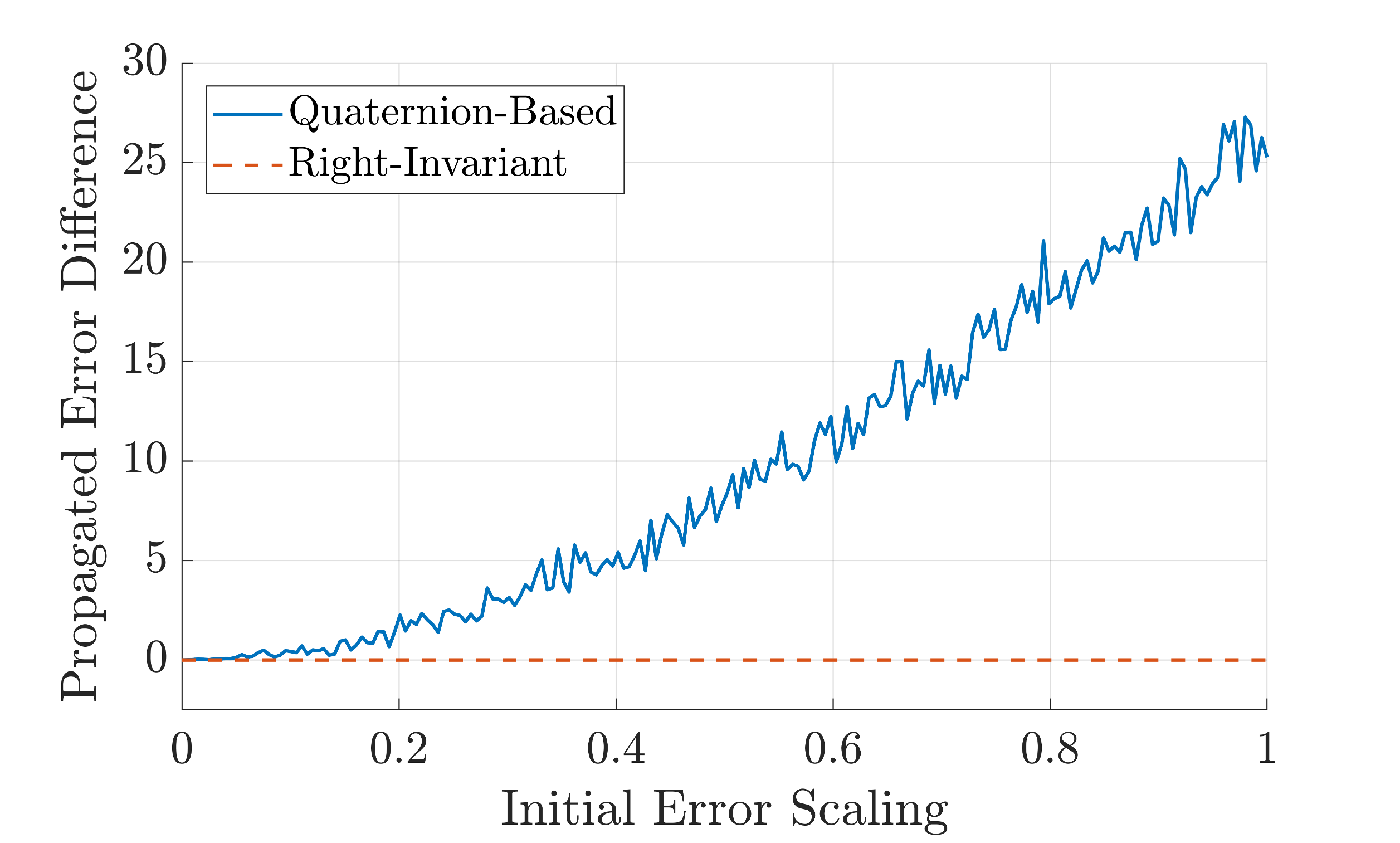
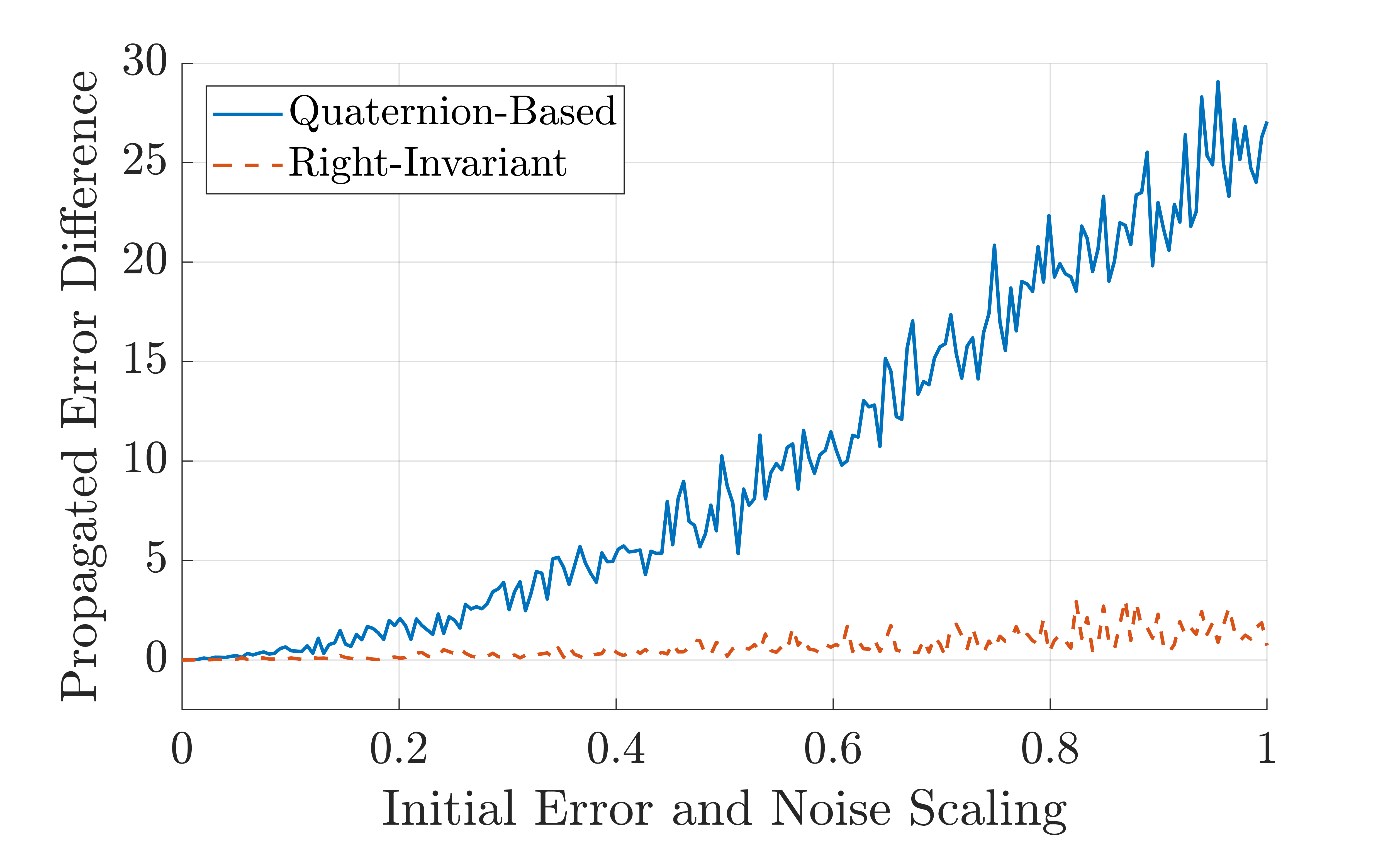
The above linearizations are clearly dependent on the state estimate. Therefore, when the estimated state deviates from the true state, the linearizations are potentially wrong, reducing accuracy and consistency in the QEKF. In contrast, the deterministic right-invariant error dynamics are exactly log-linear (14). In addition, the linearized observation matrix for our InEKF (20) is also independent of the state estimate.

Table 1: Experiment Discrete Noise Statistics and Initial Covariance
Measurement Type noise st. dev.
Linear Acceleration 0.04m/sec20.04msuperscript20.04\leavevmode\nobreak\ \mathop{\mathrm{m}}/\sec^{2}
Angular Velocity 0.002rad/sec0.002rad0.002\leavevmode\nobreak\ \mathop{\mathrm{rad}}/\sec
Accelerometer Bias 0.001m/sec30.001msuperscript30.001\leavevmode\nobreak\ \mathop{\mathrm{m}}/\sec^{3}
Gyroscope Bias 0.001rad/sec20.001radsuperscript20.001\leavevmode\nobreak\ \mathop{\mathrm{rad}}/\sec^{2}
Contact Linear Velocity 0.05m/sec0.05m0.05\leavevmode\nobreak\ \mathop{\mathrm{m}}/\sec
Joint Encoders 1.0deg1.0degree1.0\leavevmode\nobreak\ \deg
State Element initial st. dev.
Orientation of IMU 30.0deg30.0degree30.0\leavevmode\nobreak\ \deg
Velocity of IMU 1.0m/sec1.0m1.0\leavevmode\nobreak\ \mathop{\mathrm{m}}/\sec
Position of IMU 0.1m0.1m0.1\leavevmode\nobreak\ \mathop{\mathrm{m}}
Position of Right Foot 0.1m0.1m0.1\leavevmode\nobreak\ \mathop{\mathrm{m}}
Position of Left Foot 0.1m0.1m0.1\leavevmode\nobreak\ \mathop{\mathrm{m}}
Gyroscope Bias 0.005rad/sec0.005rad0.005\leavevmode\nobreak\ \mathop{\mathrm{rad}}/\sec
Accelerometer Bias 0.05m/sec20.05msuperscript20.05\leavevmode\nobreak\ \mathop{\mathrm{m}}/\sec^{2}

6.2 Convergence Comparison:

A dynamic simulation of a Cassie-series bipedal robot (described in Section 9) was performed in which the robot slowly walked forward after a small drop, accelerating from 0.00.00.0 to 0.3m/sec0.3m0.3\leavevmode\nobreak\ \mathop{\mathrm{m}}/\sec. The discrete, simulated measurements were corrupted by additive white Gaussian noise, which are specified in Table 1 along with the initial state covariance values. The same values were used in both simulation and experimental convergence evaluations of the filters. The IMU bias estimation was turned off for these simulations. The simulation was performed with MATLAB and Simulink (Simscape Multibody™) where the simulation environment models ground contact forces with a linear force law (having a stiffness and damping term) and a Coulomb friction model. A typical walking gait is shown in Figure 2.
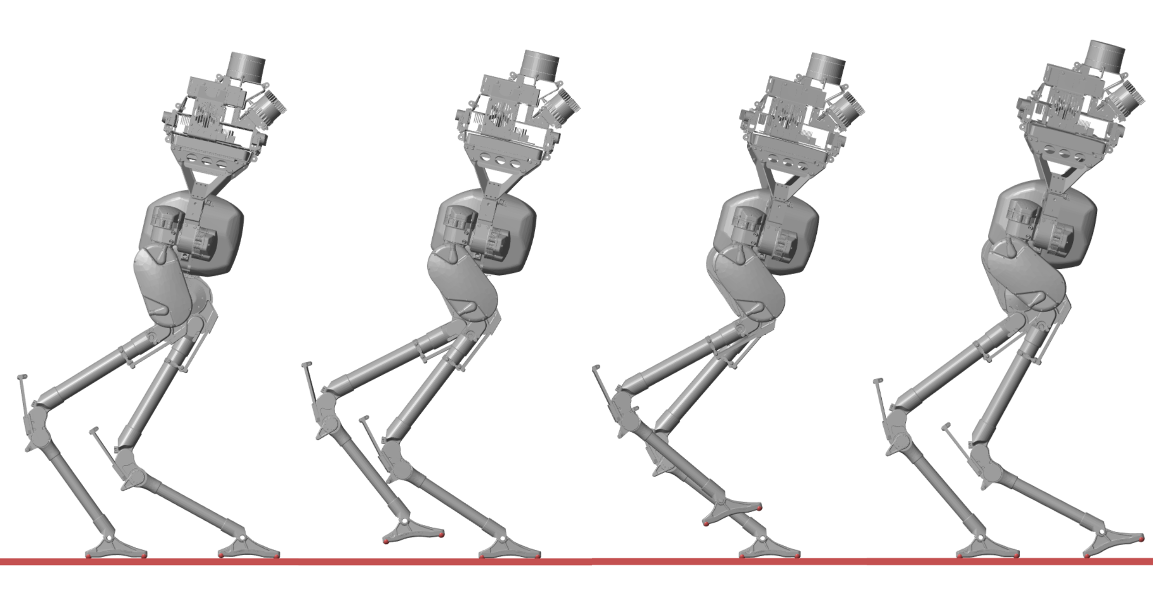
Refer to caption
Figure 2: A typical walking gait that is used for filter comparisons. The Cassie bipedal robot is simulated using Simscape Multibody™.

To compare the convergence properties of the two filters, 100 simulations of each filter were performed using identical measurements, noise statistics, initial covariance, and various random initial orientations and velocities. The initial Euler angle estimates were sampled uniformly from 30deg30degree-30\deg to 30deg30degree30\deg. The initial velocity estimates were sampled uniformly from 1.0m/sec1.0m-1.0\leavevmode\nobreak\ \mathop{\mathrm{m}}/\sec to 1.0m/sec1.0m1.0\leavevmode\nobreak\ \mathop{\mathrm{m}}/\sec. The pitch and roll estimates as well as the (body frame) velocity estimates for both filters are shown in Figure 3. Although both filters converge for this set of initial conditions, the proposed RIEKF converges considerably faster than the standard quaternion-based EKF.
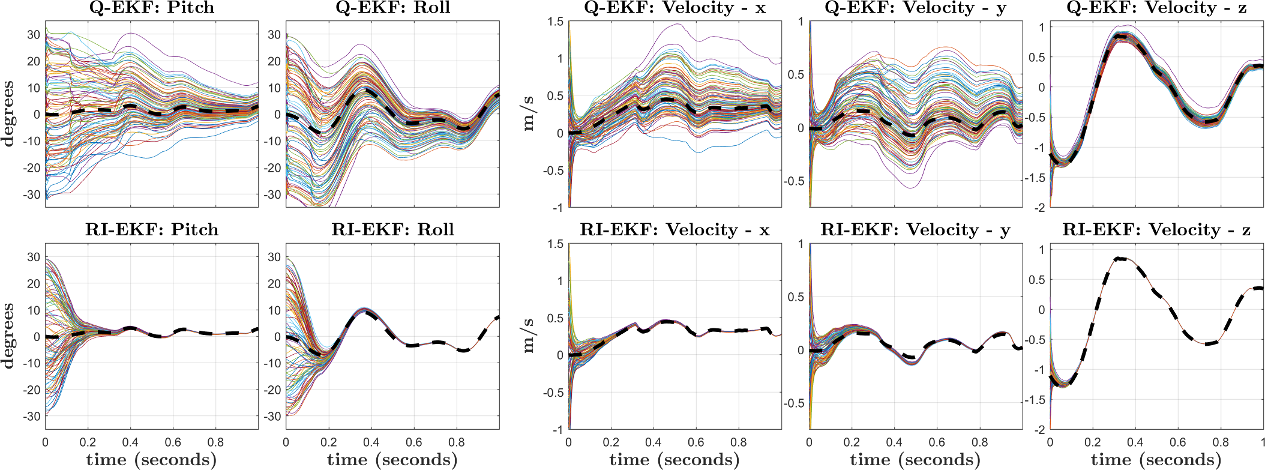
Refer to caption
Figure 3: A quaternion-based extended Kalman filter (QEKF) and the proposed right-invariant extended Kalman filter (RIEKF) were run 100 times using the same measurements, noise statistics, and initial covariance, but with random initial orientations and velocities. The noisy measurements came from a dynamic simulation of a Cassie-series biped robot where the robot walks forwards after a small drop, accelerating from 0.00.00.0 to 0.3m/sec0.3m0.3\leavevmode\nobreak\ \mathop{\mathrm{m}}/\sec. The above plots show the state estimate for the initial second of data, where the dashed black line represents the true state. The RIEKF (bottom row) converges considerably faster than the QEKF (top row) for all observable states. The estimated yaw angle (not shown) does not converge for either filter because it is unobservable. Therefore, to compare convergence, the velocities shown are represented in the estimated IMU (body) frame.

6.3 Accuracy of Linearized Dynamics

The superior performance of the InEKF over the QEKF comes from the improved accuracy of the linearized error dynamics. As indicated by Theorem 2, the deterministic error dynamics of the InEKF are actually exact, while the QEKF version is only an approximation. To demonstrate this, a simulation was performed where propagation of the true error is compared to the propagation of the linearized error dynamics.

We first analyzed the deterministic dynamics. Given an initial error vector, 𝝃0truesuperscriptsubscript𝝃0true\boldsymbol{\xi}_{0}^{\text{true}}, the initial state estimate for the InEKF was computed using the definition of right-invariant error (1), and the initial state estimate for the QEKF was computed using equation (21). The true state was initialized to the identity element. The true and estimated states for both filters were then propagated for 1 second (1000 time steps), using randomly sampled IMU measurements. The error states for both the InEKF and the QEKF were also propagated using their respective linearized error dynamics. The resulting error, 𝝃1truesuperscriptsubscript𝝃1true\boldsymbol{\xi}_{1}^{\text{true}}, between the final estimated and true states were computed and compared to the propagated error states, 𝝃1propsuperscriptsubscript𝝃1prop\boldsymbol{\xi}_{1}^{\text{prop}} to yield a measure of linearization accuracy, 𝝃1true𝝃1propdelimited-∥∥superscriptsubscript𝝃1truesuperscriptsubscript𝝃1prop\lVert\boldsymbol{\xi}_{1}^{\text{true}}-\boldsymbol{\xi}_{1}^{\text{prop}}\rVert. This test was performed multiple times while linearly scaling the initial orientation error from vec(0,0,0)vec000\mathrm{vec}(0,0,0) to vec(π/2,π/2,π/2)vec𝜋2𝜋2𝜋2\mathrm{vec}(\pi/2,\pi/2,\pi/2). The results are shown in Figure 5.

Refer to caption
Figure 4: Analyzing accuracy of the deterministic error dynamics. This Figure shows the difference between the true error and the propagated error as the initial true error increases. The state and errors were propagated for 1 second using randomly sampled IMU measurements.
Refer to caption
Figure 5: Difference between the true and propagated errors when measurements contain noise. The log-linear error dynamics of the InEKF are no longer exact.

As expected, when the initial error is zero, the difference between the true and propagated error is zero. This indicates that the linearized error dynamics for both the InEKF and the QEKF are correct. As the initial error increases, the difference between the true and propagated error states for the QEKF grows due to the decreased accuracy of the linearization. In contrast, the difference between the true and propagated error states for the InEKF are always exactly zero regardless of the initial error. In other words, assuming the initial error is known, the true propagated state can be exactly recovered from solving the linearized error dynamics system; see Theorem 2.

In the non-deterministic case (with sensor noise), Theorem 2 no longer holds. This can be seen in Figure 5, where the same test was performed, but with sensor noise corrupting the propagated state estimate. The difference between the true and propagated error is no longer exactly zero for the InEKF. However, the InEKF linearization remains more accurate due to the reduced sensitivity to initial state errors. This helps to further explain the improved convergence properties shown in Figure 3.

6.4 Covariance Ellipse Comparison

The error states in both the QEKF and the InEKF are assumed to be zero-mean Gaussian random vectors. However, due to the differing choice of error variables, the state uncertainty will differ. In the QEKF, all states and errors are decoupled (21). For example, the true position only depends on the position estimate and the position error, p=p¯+δpp¯p𝛿p\textbf{p}=\bar{\textbf{p}}+\delta\textbf{p}. Therefore, the position estimate is a Gaussian centered at p¯¯p\bar{\textbf{p}}. In contrast, when using the InEKF, the position and orientation are actually coupled together, X=exp(𝝃)X¯X𝝃¯X\textbf{X}=\exp(\boldsymbol{\xi})\bar{\textbf{X}}. Although 𝝃𝝃\boldsymbol{\xi} is a Gaussian random vector, after applying the group’s exponential map and matrix multiplication, the state estimate’s uncertainty distribution is no longer Gaussian. This distribution is known as a concentrated Gaussian on a Lie group [80, 81]. This type of distribution can often capture the underlying system uncertainty better than a standard Gaussian defined in Euclidean space [57, 7].

To demonstrate the difference, a simple simulation was performed where the Cassie robot walked forward for 8sec88\leavevmode\nobreak\ \sec at an average speed of 1m/s1𝑚𝑠1\leavevmode\nobreak\ m/s. The standard deviation for the initial position uncertainty was set to 0.1m0.1m0.1\leavevmode\nobreak\ \mathop{\mathrm{m}} about each axis, while the standard deviation of the initial yaw uncertainty was set to 10deg10degree10\leavevmode\nobreak\ \deg. A set of 10,000 particles sampled from this distribution were propagated forward to represent the robot’s true uncertainty distribution. After running both the InEKF and the QEKF, particles were sampled from the resulting filter covariances to provide a picture of the estimated position uncertainties. This result is shown in Figure 6.
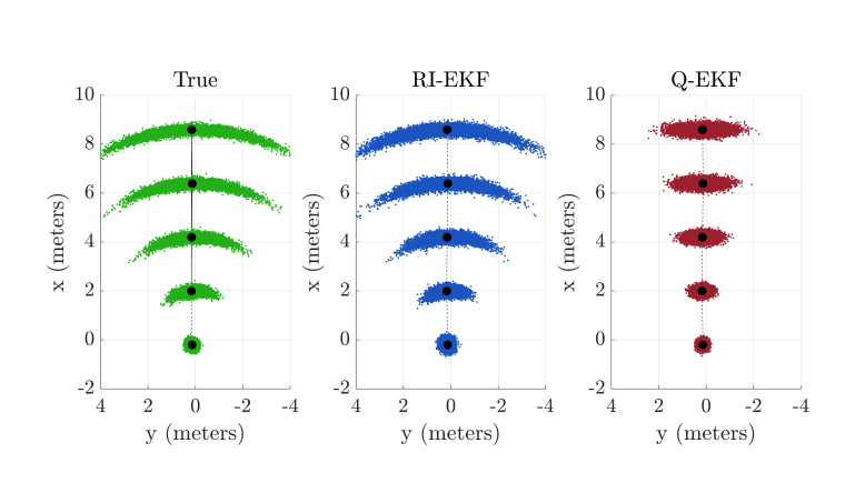
Refer to caption
Figure 6: 10,000 samples taken from the estimated filter covariances for a simulation where Cassie walked forward with an average speed of 1m/s1𝑚𝑠1\leavevmode\nobreak\ m/s. The position distributions at times 0, 2, 4, 6, and 8 sec\sec are shown.

The curved position distribution comes from the initial yaw uncertainty that continually grows due to its unobservability (Section 5.4). The InEKF is able to closely match this distribution since the samples are taken in the Lie algebra and are mapped to the group through the exponential map. This couples the orientation and position errors leading to a curved position distribution. In contrast, the QEKF position uncertainty can only have the shape of the standard Gaussian ellipse, which may not represent the true uncertainty well.

The InEKF can even accurately model the case of complete yaw uncertainty. To demonstrate this, the initial yaw standard deviation was set to 360deg360degree360\leavevmode\nobreak\ \deg, and the same 8sec88\leavevmode\nobreak\ \sec simulation was performed. Each ring in Figure 7 shows the sample position distribution spaced 2sec22\leavevmode\nobreak\ \sec apart. This type of uncertainty cannot be captured with a standard Gaussian covariance ellipse. These examples illustrate that even if the means are identical, the covariance estimate of the InEKF can provide a more accurate representation of the state’s uncertainty than the standard QEKF.
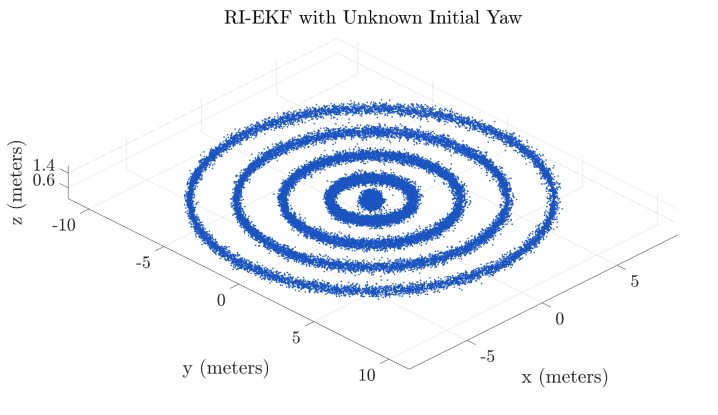
Refer to caption
Figure 7: Samples taken from the InEKF’s estimated position distribution for a walking simulation with a completely uncertain initial yaw angle. The robot moved forward at an average speed of 1 m/s𝑚𝑠m/s. Each ring represents the position uncertainty at times 0, 2, 4, 6, and 8 sec\sec.

In these examples, the initial covariance of all states (except yaw) was small. It is interesting to note what happens if we remove the dynamics noise and set the covariance for some states to exactly zero (rank-deficient covariance matrix). In this case, the initial covariance is supported by a subgroup and the InEKF will keep the state estimate within a time-dependent subset of the Lie group at all times. This theoretical result was proved by Chauchat et al. [25], Barrau and Bonnabel [12] to create EKFs with state equality constraints.

7 IMU bias augmentation

Implementation of an IMU-based state estimator on hardware typically requires modeling additional states, such as gyroscope and accelerometer biases. Unfortunately, as noted in Barrau [8], there is no Lie group that includes the bias terms while also having the dynamics satisfy the group affine property (2). Even though many of the theoretical properties of the RIEKF will no longer hold, it is possible to design an “imperfect InEKF” that still outperforms the standard EKF [8].

7.1 State Representation

The IMU biases are slowly varying signals that corrupt the measurements in an additive manner:

𝝎~tsubscript~𝝎𝑡\displaystyle\tilde{\boldsymbol{\omega}}_{t} =𝝎t+btg+wtg,absentsubscript𝝎𝑡superscriptsubscriptb𝑡𝑔superscriptsubscriptw𝑡𝑔\displaystyle=\boldsymbol{\omega}_{t}+\textbf{b}_{t}^{g}+\textbf{w}_{t}^{g},\qquad wtg𝒢𝒫(03,1,𝚺gδ(tt))similar-tosuperscriptsubscriptw𝑡𝑔𝒢𝒫subscript031superscript𝚺𝑔𝛿𝑡superscript𝑡\displaystyle\textbf{w}_{t}^{g}\sim\mathcal{GP}\left(\textbf{0}_{3,1},\boldsymbol{\Sigma}^{g}\,\delta(t-t^{\prime})\right)
a~tsubscript~a𝑡\displaystyle\tilde{\textbf{a}}_{t} =at+bta+wta,absentsubscripta𝑡superscriptsubscriptb𝑡𝑎superscriptsubscriptw𝑡𝑎\displaystyle=\textbf{a}_{t}+\textbf{b}_{t}^{a}+\textbf{w}_{t}^{a},\qquad wta𝒢𝒫(03,1,𝚺aδ(tt)).similar-tosuperscriptsubscriptw𝑡𝑎𝒢𝒫subscript031superscript𝚺𝑎𝛿𝑡superscript𝑡\displaystyle\textbf{w}_{t}^{a}\sim\mathcal{GP}\left(\textbf{0}_{3,1},\boldsymbol{\Sigma}^{a}\,\delta(t-t^{\prime})\right).

These biases form a parameter vector that needs to be estimated as part of the RIEKF state,

𝜽t[bg(t)ba(t)][btgbta]6.subscript𝜽𝑡matrixsuperscriptb𝑔𝑡superscriptb𝑎𝑡matrixsuperscriptsubscriptb𝑡𝑔superscriptsubscriptb𝑡𝑎superscript6\begin{split}\boldsymbol{\theta}_{t}&\triangleq\begin{bmatrix}\textbf{b}^{g}(t)\\ \textbf{b}^{a}(t)\\ \end{bmatrix}\triangleq\begin{bmatrix}\textbf{b}_{t}^{g}\\ \textbf{b}_{t}^{a}\\ \end{bmatrix}\in\mathbb{R}^{6}.\end{split} (22)

The model’s state now becomes a tuple of our original matrix Lie group and the parameter vector, (Xt,𝜽t)𝒢×6subscriptX𝑡subscript𝜽𝑡𝒢superscript6(\textbf{X}_{t},\boldsymbol{\theta}_{t})\in\mathcal{G}\times\mathbb{R}^{6}. The augmented right-invariant error is now defined as

etr(X¯tXt1,𝜽¯t𝜽t)(𝜼tr,𝜻t).superscriptsubscripte𝑡𝑟subscript¯X𝑡superscriptsubscriptX𝑡1subscript¯𝜽𝑡subscript𝜽𝑡superscriptsubscript𝜼𝑡𝑟subscript𝜻𝑡\textbf{e}_{t}^{r}\triangleq(\bar{\textbf{X}}_{t}\textbf{X}_{t}^{-1},\bar{\boldsymbol{\theta}}_{t}-\boldsymbol{\theta}_{t})\triangleq(\boldsymbol{\eta}_{t}^{r},\boldsymbol{\zeta}_{t}). (23)

Written explicitly, the right-invariant error is

𝜼tr=[R¯tRt𝖳v¯tR¯tRt𝖳vtp¯tR¯tRt𝖳ptd¯tR¯tRt𝖳dt01,310001,301001,3001],superscriptsubscript𝜼𝑡𝑟matrixsubscript¯R𝑡superscriptsubscriptR𝑡𝖳subscript¯v𝑡subscript¯R𝑡superscriptsubscriptR𝑡𝖳subscriptv𝑡subscript¯p𝑡subscript¯R𝑡superscriptsubscriptR𝑡𝖳subscriptp𝑡subscript¯d𝑡subscript¯R𝑡superscriptsubscriptR𝑡𝖳subscriptd𝑡subscript013100subscript013010subscript013001\boldsymbol{\eta}_{t}^{r}=\begin{bmatrix}\bar{\textbf{R}}_{t}\textbf{R}_{t}^{\mathsf{T}}&\bar{\textbf{v}}_{t}-\bar{\textbf{R}}_{t}\textbf{R}_{t}^{\mathsf{T}}\textbf{v}_{t}&\bar{\textbf{p}}_{t}-\bar{\textbf{R}}_{t}\textbf{R}_{t}^{\mathsf{T}}\textbf{p}_{t}&\bar{\textbf{d}}_{t}-\bar{\textbf{R}}_{t}\textbf{R}_{t}^{\mathsf{T}}\textbf{d}_{t}\\ \textbf{0}_{1,3}&1&0&0\\ \textbf{0}_{1,3}&0&1&0\\ \textbf{0}_{1,3}&0&0&1\\ \end{bmatrix},

while the parameter vector error is given by

𝜻t=[b¯tgbtgb¯tabta][𝜻tg𝜻ta].subscript𝜻𝑡matrixsuperscriptsubscript¯b𝑡𝑔superscriptsubscriptb𝑡𝑔superscriptsubscript¯b𝑡𝑎superscriptsubscriptb𝑡𝑎matrixsuperscriptsubscript𝜻𝑡𝑔superscriptsubscript𝜻𝑡𝑎\boldsymbol{\zeta}_{t}=\begin{bmatrix}\bar{\textbf{b}}_{t}^{g}-\textbf{b}_{t}^{g}\\ \bar{\textbf{b}}_{t}^{a}-\textbf{b}_{t}^{a}\\ \end{bmatrix}\triangleq\begin{bmatrix}\boldsymbol{\zeta}_{t}^{g}\\ \boldsymbol{\zeta}_{t}^{a}\end{bmatrix}.

7.2 System Dynamics

With IMU biases included, the system dynamics are now expressed as

ddtRt=Rt(𝝎~tbtgwtg)×ddtvt=Rt(a~tbtawta)+gddtpt=vtddtdt=RthR(𝜶~t)(wtv).dd𝑡subscriptR𝑡subscriptR𝑡subscriptsubscript~𝝎𝑡superscriptsubscriptb𝑡𝑔superscriptsubscriptw𝑡𝑔dd𝑡subscriptv𝑡subscriptR𝑡subscript~a𝑡superscriptsubscriptb𝑡𝑎superscriptsubscriptw𝑡𝑎gdd𝑡subscriptp𝑡subscriptv𝑡dd𝑡subscriptd𝑡subscriptR𝑡subscripth𝑅subscript~𝜶𝑡superscriptsubscriptw𝑡𝑣\begin{split}\dfrac{\mathrm{d}}{\mathrm{d}t}\textbf{R}_{t}&=\textbf{R}_{t}\left(\tilde{\boldsymbol{\omega}}_{t}-\textbf{b}_{t}^{g}-\textbf{w}_{t}^{g}\right)_{\times}\\ \dfrac{\mathrm{d}}{\mathrm{d}t}\textbf{v}_{t}&=\textbf{R}_{t}(\tilde{\textbf{a}}_{t}-\textbf{b}_{t}^{a}-\textbf{w}_{t}^{a})+\textbf{g}\\ \dfrac{\mathrm{d}}{\mathrm{d}t}\textbf{p}_{t}&=\textbf{v}_{t}\\ \dfrac{\mathrm{d}}{\mathrm{d}t}\textbf{d}_{t}&=\textbf{R}_{t}\;\textit{{h}}_{R}(\tilde{\boldsymbol{\alpha}}_{t})(-\textbf{w}_{t}^{v}).\end{split} (24)

The IMU bias dynamics are modeled using the typical “Brownian motion” model, i.e., the derivatives are white Gaussian noise, to capture the slowly time-varying nature of these parameters,

ddtbtgdd𝑡superscriptsubscriptb𝑡𝑔\displaystyle\dfrac{\mathrm{d}}{\mathrm{d}t}\textbf{b}_{t}^{g} =wtbg,absentsuperscriptsubscriptw𝑡𝑏𝑔\displaystyle=\textbf{w}_{t}^{bg},\quad wtbg𝒢𝒫(03,1,𝚺bgδ(tt))similar-tosuperscriptsubscriptw𝑡𝑏𝑔𝒢𝒫subscript031superscript𝚺𝑏𝑔𝛿𝑡superscript𝑡\displaystyle\textbf{w}_{t}^{bg}\sim\mathcal{GP}(\textbf{0}_{3,1},\boldsymbol{\Sigma}^{bg}\,\delta(t-t^{\prime})) (25)
ddtbtadd𝑡superscriptsubscriptb𝑡𝑎\displaystyle\dfrac{\mathrm{d}}{\mathrm{d}t}\textbf{b}_{t}^{a} =wtba,absentsuperscriptsubscriptw𝑡𝑏𝑎\displaystyle=\textbf{w}_{t}^{ba},\quad wtba𝒢𝒫(03,1,𝚺baδ(tt)).similar-tosuperscriptsubscriptw𝑡𝑏𝑎𝒢𝒫subscript031superscript𝚺𝑏𝑎𝛿𝑡superscript𝑡\displaystyle\textbf{w}_{t}^{ba}\sim\mathcal{GP}(\textbf{0}_{3,1},\boldsymbol{\Sigma}^{ba}\,\delta(t-t^{\prime})).

The deterministic system dynamics now depend on both the inputs, utsubscriptu𝑡\textbf{u}_{t}, and the parameters, 𝜽tsubscript𝜽𝑡\boldsymbol{\theta}_{t}

fut(X¯t,𝜽¯t)=[R¯t(𝝎¯t)×R¯ta¯t+gv¯t03,101,300001,300001,3000],subscript𝑓subscriptu𝑡subscript¯X𝑡subscript¯𝜽𝑡matrixsubscript¯R𝑡subscriptsubscript¯𝝎𝑡subscript¯R𝑡subscript¯a𝑡gsubscript¯v𝑡subscript031subscript013000subscript013000subscript013000f_{\textbf{u}_{t}}(\bar{\textbf{X}}_{t},\bar{\boldsymbol{\theta}}_{t})=\begin{bmatrix}\bar{\textbf{R}}_{t}\left(\bar{\boldsymbol{\omega}}_{t}\right)_{\times}&\bar{\textbf{R}}_{t}\bar{\textbf{a}}_{t}+\textbf{g}&\bar{\textbf{v}}_{t}&\textbf{0}_{3,1}\\ \textbf{0}_{1,3}&0&0&0\\ \textbf{0}_{1,3}&0&0&0\\ \textbf{0}_{1,3}&0&0&0\\ \end{bmatrix},

where 𝝎¯t𝝎~tb¯tgsubscript¯𝝎𝑡subscript~𝝎𝑡superscriptsubscript¯b𝑡𝑔\bar{\boldsymbol{\omega}}_{t}\triangleq\tilde{\boldsymbol{\omega}}_{t}-\bar{\textbf{b}}_{t}^{g} and a¯ta~tb¯tasubscript¯a𝑡subscript~a𝑡superscriptsubscript¯b𝑡𝑎\bar{\textbf{a}}_{t}\triangleq\tilde{\textbf{a}}_{t}-\bar{\textbf{b}}_{t}^{a} are the “bias-corrected” inputs. To compute the linearized error dynamics, the augmented right-invariant error (23) is first differentiated with respect to time,

ddtetr=(ddt𝜼tr,[wtbgwtba]).dd𝑡superscriptsubscripte𝑡𝑟dd𝑡superscriptsubscript𝜼𝑡𝑟matrixsuperscriptsubscriptw𝑡𝑏𝑔superscriptsubscriptw𝑡𝑏𝑎\begin{split}\dfrac{\mathrm{d}}{\mathrm{d}t}\textbf{e}_{t}^{r}&=\left(\dfrac{\mathrm{d}}{\mathrm{d}t}\boldsymbol{\eta}_{t}^{r},\begin{bmatrix}\textbf{w}_{t}^{bg}\\ \textbf{w}_{t}^{ba}\\ \end{bmatrix}\right).\end{split} (26)

After carrying out the chain rule and making the first order approximation, 𝜼tr=exp(𝝃t)Id+𝝃tsuperscriptsubscript𝜼𝑡𝑟subscript𝝃𝑡subscriptI𝑑superscriptsubscript𝝃𝑡\boldsymbol{\eta}_{t}^{r}=\exp(\boldsymbol{\xi}_{t})\approx\textbf{{I}}_{d}+{\boldsymbol{\xi}_{t}}^{\wedge}, the individual terms of the invariant error dynamics become

ddt(R¯tRt𝖳)(R¯t(wtg𝜻tg))×ddt(v¯tR¯tRt𝖳vt)(g)×𝝃tR+(v¯t)×R¯t(wtg𝜻tg)+R¯t(wta𝜻ta)ddt(p¯tR¯tRt𝖳pt)𝝃tv+(p¯t)×R¯t(wtg𝜻tg)ddt(d¯tR¯tRt𝖳dt)(d¯t)×R¯t(wtg𝜻tg)+R¯thR(𝜶~t)wtv.dd𝑡subscript¯R𝑡superscriptsubscriptR𝑡𝖳subscriptsubscript¯R𝑡superscriptsubscriptw𝑡𝑔superscriptsubscript𝜻𝑡𝑔dd𝑡subscript¯v𝑡subscript¯R𝑡superscriptsubscriptR𝑡𝖳subscriptv𝑡subscriptgsuperscriptsubscript𝝃𝑡𝑅subscriptsubscript¯v𝑡subscript¯R𝑡superscriptsubscriptw𝑡𝑔superscriptsubscript𝜻𝑡𝑔subscript¯R𝑡superscriptsubscriptw𝑡𝑎superscriptsubscript𝜻𝑡𝑎dd𝑡subscript¯p𝑡subscript¯R𝑡superscriptsubscriptR𝑡𝖳subscriptp𝑡superscriptsubscript𝝃𝑡𝑣subscriptsubscript¯p𝑡subscript¯R𝑡superscriptsubscriptw𝑡𝑔superscriptsubscript𝜻𝑡𝑔dd𝑡subscript¯d𝑡subscript¯R𝑡superscriptsubscriptR𝑡𝖳subscriptd𝑡subscriptsubscript¯d𝑡subscript¯R𝑡superscriptsubscriptw𝑡𝑔superscriptsubscript𝜻𝑡𝑔subscript¯R𝑡subscripth𝑅subscript~𝜶𝑡superscriptsubscriptw𝑡𝑣\begin{split}\dfrac{\mathrm{d}}{\mathrm{d}t}\left(\bar{\textbf{R}}_{t}\textbf{R}_{t}^{\mathsf{T}}\right)&\approx\left(\bar{\textbf{R}}_{t}\left(\textbf{w}_{t}^{g}-\boldsymbol{\zeta}_{t}^{g}\right)\right)_{\times}\\ \dfrac{\mathrm{d}}{\mathrm{d}t}\left(\bar{\textbf{v}}_{t}-\bar{\textbf{R}}_{t}\textbf{R}_{t}^{\mathsf{T}}\textbf{v}_{t}\right)&\approx\left(\textbf{g}\right)_{\times}\boldsymbol{\xi}_{t}^{R}+\left(\bar{\textbf{v}}_{t}\right)_{\times}\bar{\textbf{R}}_{t}(\textbf{w}_{t}^{g}-\boldsymbol{\zeta}_{t}^{g})+\bar{\textbf{R}}_{t}(\textbf{w}_{t}^{a}-\boldsymbol{\zeta}_{t}^{a})\\ \dfrac{\mathrm{d}}{\mathrm{d}t}\left(\bar{\textbf{p}}_{t}-\bar{\textbf{R}}_{t}\textbf{R}_{t}^{\mathsf{T}}\textbf{p}_{t}\right)&\approx\boldsymbol{\xi}_{t}^{v}+\left(\bar{\textbf{p}}_{t}\right)_{\times}\bar{\textbf{R}}_{t}(\textbf{w}_{t}^{g}-\boldsymbol{\zeta}_{t}^{g})\\ \dfrac{\mathrm{d}}{\mathrm{d}t}\left(\bar{\textbf{d}}_{t}-\bar{\textbf{R}}_{t}\textbf{R}_{t}^{\mathsf{T}}\textbf{d}_{t}\right)&\approx\left(\bar{\textbf{d}}_{t}\right)_{\times}\bar{\textbf{R}}_{t}(\textbf{w}_{t}^{g}-\boldsymbol{\zeta}_{t}^{g})+\bar{\textbf{R}}_{t}\;\textit{{h}}_{R}(\tilde{\boldsymbol{\alpha}}_{t})\textbf{w}_{t}^{v}.\end{split} (27)

Importantly, the augmented invariant error dynamics only depends on the estimated trajectory though the noise and bias errors, 𝜻tsubscript𝜻𝑡\boldsymbol{\zeta}_{t} (this is expected because when there are no bias errors, there is no dependence on the estimated trajectory). A linear system can now be constructed from (27) to yield,

ddt[𝝃t𝜻t]=At[𝝃t𝜻t]+[AdX¯t012,606,12I6]wt,dd𝑡matrixsubscript𝝃𝑡subscript𝜻𝑡subscriptA𝑡matrixsubscript𝝃𝑡subscript𝜻𝑡matrixsubscriptAdsubscript¯X𝑡subscript0126subscript0612subscriptI6subscriptw𝑡\dfrac{\mathrm{d}}{\mathrm{d}t}\begin{bmatrix}\boldsymbol{\xi}_{t}\\ \boldsymbol{\zeta}_{t}\end{bmatrix}=\textbf{A}_{t}\begin{bmatrix}\boldsymbol{\xi}_{t}\\ \boldsymbol{\zeta}_{t}\end{bmatrix}+\begin{bmatrix}\mathrm{Ad}_{\bar{\textbf{X}}_{t}}&\textbf{0}_{12,6}\\ \textbf{0}_{6,12}&\textbf{I}_{6}\end{bmatrix}\textbf{w}_{t},

where the noise vector is augmented to include the bias terms,

wtvec(wtg,wta,03,1,hR(𝜶~t)wtv,wtbg,wtba).subscriptw𝑡vecsuperscriptsubscriptw𝑡𝑔superscriptsubscriptw𝑡𝑎subscript031subscripth𝑅subscript~𝜶𝑡superscriptsubscriptw𝑡𝑣superscriptsubscriptw𝑡𝑏𝑔superscriptsubscriptw𝑡𝑏𝑎\textbf{w}_{t}\triangleq\mathrm{vec}(\textbf{w}_{t}^{g},\,\textbf{w}_{t}^{a},\,\textbf{0}_{3,1},\;\textit{{h}}_{R}(\tilde{\boldsymbol{\alpha}}_{t})\textbf{w}_{t}^{v},\textbf{w}_{t}^{bg},\textbf{w}_{t}^{ba}).

7.3 Forward Kinematic Measurements

The forward kinematics position measurement (17) does not depend on the IMU biases. Therefore, the HtsubscriptH𝑡\textbf{H}_{t} matrix can simply be appended with zeros to account for the augmented variables. The linear update equation becomes

[𝝃t+𝜻t+]=[𝝃t𝜻t][Kt𝝃Kt𝜻](Ht[𝝃t𝜻t]R¯t(Jp(𝜶~t)wtα)).matrixsuperscriptsubscript𝝃𝑡superscriptsubscript𝜻𝑡matrixsubscript𝝃𝑡subscript𝜻𝑡matrixsuperscriptsubscriptK𝑡𝝃superscriptsubscriptK𝑡𝜻subscriptH𝑡matrixsubscript𝝃𝑡subscript𝜻𝑡subscript¯R𝑡subscriptJ𝑝subscript~𝜶𝑡superscriptsubscriptw𝑡𝛼\begin{bmatrix}\boldsymbol{\xi}_{t}^{+}\\ \boldsymbol{\zeta}_{t}^{+}\end{bmatrix}=\begin{bmatrix}\boldsymbol{\xi}_{t}\\ \boldsymbol{\zeta}_{t}\end{bmatrix}-\begin{bmatrix}\textbf{K}_{t}^{\boldsymbol{\xi}}\\ \textbf{K}_{t}^{\boldsymbol{\zeta}}\end{bmatrix}\left(\textbf{H}_{t}\begin{bmatrix}\boldsymbol{\xi}_{t}\\ \boldsymbol{\zeta}_{t}\end{bmatrix}-\bar{\textbf{R}}_{t}\left(\textbf{J}_{p}(\tilde{\boldsymbol{\alpha}}_{t})\textbf{w}_{t}^{\alpha}\right)\right).

7.4 Final Continuous RIEKF Equations

The final “imperfect” RIEKF equations that include IMU biases can now be written down. The estimated state tuple is predicted using the following set of differential equations:

ddt(X¯t,𝜽¯t)=(fut(X¯t,𝜽¯t),06,1).dd𝑡subscript¯X𝑡subscript¯𝜽𝑡subscript𝑓subscriptu𝑡subscript¯X𝑡subscript¯𝜽𝑡subscript061\dfrac{\mathrm{d}}{\mathrm{d}t}\left(\bar{\textbf{X}}_{t}\,,\bar{\boldsymbol{\theta}}_{t}\right)=\left(f_{\textbf{u}_{t}}(\bar{\textbf{X}}_{t},\bar{\boldsymbol{\theta}}_{t}),\textbf{0}_{6,1}\right).

The covariance of the augmented right invariant error dynamics is computed by solving the Riccati equation

ddtPt=AtPt+PtAt𝖳+Q¯t,dd𝑡subscriptP𝑡subscriptA𝑡subscriptP𝑡subscriptP𝑡superscriptsubscriptA𝑡𝖳subscript¯Q𝑡\dfrac{\mathrm{d}}{\mathrm{d}t}\textbf{P}_{t}=\textbf{A}_{t}\textbf{P}_{t}+\textbf{P}_{t}\textbf{A}_{t}^{\mathsf{T}}+\bar{\textbf{Q}}_{t},

where the matrices AtsubscriptA𝑡\textbf{A}_{t} and Q¯tsubscript¯Q𝑡\bar{\textbf{Q}}_{t} are now defined using (27),

At=[0000R¯t0(g)×000(v¯t)×R¯tR¯t0I00(p¯t)×R¯t00000(d¯t)×R¯t0000000000000]Q¯t=[AdX¯t012,606,12I6]Cov(wt)[AdX¯t012,606,12I6]𝖳.subscriptA𝑡matrix0000subscript¯R𝑡0subscriptg000subscriptsubscript¯v𝑡subscript¯R𝑡subscript¯R𝑡0I00subscriptsubscript¯p𝑡subscript¯R𝑡00000subscriptsubscript¯d𝑡subscript¯R𝑡0000000000000subscript¯Q𝑡matrixsubscriptAdsubscript¯X𝑡subscript0126subscript0612subscriptI6Covsubscriptw𝑡superscriptmatrixsubscriptAdsubscript¯X𝑡subscript0126subscript0612subscriptI6𝖳\begin{split}\textbf{A}_{t}&=\begin{bmatrix}\textbf{0}&\textbf{0}&\textbf{0}&\textbf{0}&-\bar{\textbf{R}}_{t}&\textbf{0}\\ \left(\textbf{g}\right)_{\times}&\textbf{0}&\textbf{0}&\textbf{0}&-\left(\bar{\textbf{v}}_{t}\right)_{\times}\bar{\textbf{R}}_{t}&-\bar{\textbf{R}}_{t}\\ \textbf{0}&\textbf{I}&\textbf{0}&\textbf{0}&-\left(\bar{\textbf{p}}_{t}\right)_{\times}\bar{\textbf{R}}_{t}&\textbf{0}\\ \textbf{0}&\textbf{0}&\textbf{0}&\textbf{0}&-\left(\bar{\textbf{d}}_{t}\right)_{\times}\bar{\textbf{R}}_{t}&\textbf{0}\\ \textbf{0}&\textbf{0}&\textbf{0}&\textbf{0}&\textbf{0}&\textbf{0}\\ \textbf{0}&\textbf{0}&\textbf{0}&\textbf{0}&\textbf{0}&\textbf{0}\\ \end{bmatrix}\\ \bar{\textbf{Q}}_{t}&=\begin{bmatrix}\mathrm{Ad}_{\bar{\textbf{X}}_{t}}&\textbf{0}_{12,6}\\ \textbf{0}_{6,12}&\textbf{I}_{6}\end{bmatrix}\text{Cov}(\textbf{w}_{t})\begin{bmatrix}\mathrm{Ad}_{\bar{\textbf{X}}_{t}}&\textbf{0}_{12,6}\\ \textbf{0}_{6,12}&\textbf{I}_{6}\end{bmatrix}^{\mathsf{T}}.\\ \end{split} (28)

The estimated state tuple and its covariance are corrected though the update equations

(X¯t+,𝜽t+)=(exp(Kt𝝃𝚷X¯tYt)X¯t,𝜽¯t+Kt𝜻𝚷X¯tYt)Pt+=(IKtHt)Pt(IKtHt)𝖳+KtN¯tKt𝖳,superscriptsubscript¯X𝑡superscriptsubscript𝜽𝑡superscriptsubscriptK𝑡𝝃𝚷subscript¯X𝑡subscriptY𝑡subscript¯X𝑡subscript¯𝜽𝑡superscriptsubscriptK𝑡𝜻𝚷subscript¯X𝑡subscriptY𝑡superscriptsubscriptP𝑡IsubscriptK𝑡subscriptH𝑡subscriptP𝑡superscriptIsubscriptK𝑡subscriptH𝑡𝖳subscriptK𝑡subscript¯N𝑡superscriptsubscriptK𝑡𝖳\begin{split}\left(\bar{\textbf{X}}_{t}^{+},\boldsymbol{\theta}_{t}^{+}\right)&=\left(\exp\left(\textbf{K}_{t}^{\boldsymbol{\xi}}\boldsymbol{\Pi}\bar{\textbf{X}}_{t}\textbf{Y}_{t}\right)\bar{\textbf{X}}_{t}\,,\;\;\bar{\boldsymbol{\theta}}_{t}+\textbf{K}_{t}^{\boldsymbol{\zeta}}\boldsymbol{\Pi}\bar{\textbf{X}}_{t}\textbf{Y}_{t}\right)\\ \textbf{P}_{t}^{+}&=(\textbf{I}-\textbf{K}_{t}\textbf{H}_{t})\textbf{P}_{t}(\textbf{I}-\textbf{K}_{t}\textbf{H}_{t})^{\mathsf{T}}+\textbf{K}_{t}\bar{\textbf{N}}_{t}\textbf{K}_{t}^{\mathsf{T}},\end{split} (29)

where the gains Kt𝝃superscriptsubscriptK𝑡𝝃\textbf{K}_{t}^{\boldsymbol{\xi}} and Kt𝜻superscriptsubscriptK𝑡𝜻\textbf{K}_{t}^{\boldsymbol{\zeta}} are computed from

St=HtPtHt𝖳+N¯tKt=[Kt𝝃Kt𝜻]=PtHt𝖳St1,formulae-sequencesubscriptS𝑡subscriptH𝑡subscriptP𝑡superscriptsubscriptH𝑡𝖳subscript¯N𝑡subscriptK𝑡matrixsuperscriptsubscriptK𝑡𝝃superscriptsubscriptK𝑡𝜻subscriptP𝑡superscriptsubscriptH𝑡𝖳superscriptsubscriptS𝑡1\displaystyle\textbf{S}_{t}=\textbf{H}_{t}\textbf{P}_{t}\textbf{H}_{t}^{\mathsf{T}}+\bar{\textbf{N}}_{t}\qquad\textbf{K}_{t}=\begin{bmatrix}\textbf{K}_{t}^{\boldsymbol{\xi}}\\ \textbf{K}_{t}^{\boldsymbol{\zeta}}\end{bmatrix}=\textbf{P}_{t}\textbf{H}_{t}^{\mathsf{T}}\textbf{S}_{t}^{-1},

with the following measurement, output, and noise matrices,

Yt𝖳=[hp𝖳(𝜶~t)011],Ht=[00II00],N¯t=R¯tJp(𝜶~t)Cov(wtα)Jp𝖳(𝜶~t)R¯t𝖳.formulae-sequencesuperscriptsubscriptY𝑡𝖳matrixsuperscriptsubscripth𝑝𝖳subscript~𝜶𝑡011formulae-sequencesubscriptH𝑡matrix00II00subscript¯N𝑡subscript¯R𝑡subscriptJ𝑝subscript~𝜶𝑡Covsuperscriptsubscriptw𝑡𝛼superscriptsubscriptJ𝑝𝖳subscript~𝜶𝑡superscriptsubscript¯R𝑡𝖳\begin{split}\textbf{Y}_{t}^{\mathsf{T}}&=\begin{bmatrix}\;\textit{{h}}_{p}^{\mathsf{T}}(\tilde{\boldsymbol{\alpha}}_{t})&0&1&-1\end{bmatrix},\\ \textbf{H}_{t}&=\begin{bmatrix}\textbf{0}&\textbf{0}&-\textbf{I}&\textbf{I}&\textbf{0}&\textbf{0}\end{bmatrix},\\ \bar{\textbf{N}}_{t}&=\bar{\textbf{R}}_{t}\;\textbf{J}_{p}(\tilde{\boldsymbol{\alpha}}_{t})\;\text{Cov}(\textbf{w}_{t}^{\alpha})\;\textbf{J}_{p}^{\mathsf{T}}(\tilde{\boldsymbol{\alpha}}_{t})\;\bar{\textbf{R}}_{t}^{\mathsf{T}}.\end{split}
Remark 3.

The upper-right block of the new linearized dynamics matrix (28) is related to the adjoint of the current state estimate (7). Intuitively, this maps the bias error (measured in the body frame) to the world frame.

8 Addition and Removal of Contact Points

Sections 5 and 7 derived the equations for the RIEKF under the assumption that the contact point is unchanging with time. However, for legged robots, contacts are discrete events that are created and broken as a robot navigates through the environment. Therefore, it is important to be able to conveniently add and remove contact points states to and from the observer’s state.

8.1 Removing Contact Points

To remove a previous contact point from the state, we marginalize the corresponding state variable by simply removing the corresponding column and row from the matrix Lie group. The corresponding elements of the covariance matrix are also eliminated. This can be done through a simple linear transformation. For example, if the robot is going from one contact to zero contacts, then the newly reduced covariance would be computed by

[𝝃tR𝝃tv𝝃tp]=[I0000I0000I0][𝝃tR𝝃tv𝝃tp𝝃td]𝝃tnewM𝝃tPtnew=MPtM𝖳.matrixsuperscriptsubscript𝝃𝑡𝑅superscriptsubscript𝝃𝑡𝑣superscriptsubscript𝝃𝑡𝑝matrixI0000I0000I0matrixsuperscriptsubscript𝝃𝑡𝑅superscriptsubscript𝝃𝑡𝑣superscriptsubscript𝝃𝑡𝑝superscriptsubscript𝝃𝑡𝑑superscriptsubscript𝝃𝑡newMsubscript𝝃𝑡superscriptsubscriptP𝑡newMsubscriptP𝑡superscriptM𝖳\begin{split}\begin{bmatrix}\boldsymbol{\xi}_{t}^{R}\\ \boldsymbol{\xi}_{t}^{v}\\ \boldsymbol{\xi}_{t}^{p}\\ \end{bmatrix}&=\begin{bmatrix}\textbf{I}&\textbf{0}&\textbf{0}&\textbf{0}\\ \textbf{0}&\textbf{I}&\textbf{0}&\textbf{0}\\ \textbf{0}&\textbf{0}&\textbf{I}&\textbf{0}\\ \end{bmatrix}\begin{bmatrix}\boldsymbol{\xi}_{t}^{R}\\ \boldsymbol{\xi}_{t}^{v}\\ \boldsymbol{\xi}_{t}^{p}\\ \boldsymbol{\xi}_{t}^{d}\\ \end{bmatrix}\\ \boldsymbol{\xi}_{t}^{\mathrm{new}}&\triangleq\textbf{M}\,\boldsymbol{\xi}_{t}\\ \implies\textbf{P}_{t}^{\mathrm{new}}&=\textbf{M}\,\textbf{P}_{t}\,\textbf{M}^{\mathsf{T}}.\end{split} (30)
Remark 4.

This marginalization matrix, M, does not depend on the choice of right or left invariant error.

8.2 Adding Contact Points

When the robot makes a new contact with the environment, the state and covariance matrices need to be augmented. Special attention needs to be given to initialize the mean and covariance for the new estimated contact point. For example, if the robot is going from zero contacts to one contact, the initial mean is obtained though the forward kinematics relation

d¯t=p¯t+R¯thp(𝜶~t).subscript¯d𝑡subscript¯p𝑡subscript¯R𝑡subscripth𝑝subscript~𝜶𝑡\bar{\textbf{d}}_{t}=\bar{\textbf{p}}_{t}+\bar{\textbf{R}}_{t}\;\textit{{h}}_{p}(\tilde{\boldsymbol{\alpha}}_{t}). (31)

In order to compute the new covariance, we need to look at the right-invariant error,

𝜼td=d¯tR¯tRt𝖳dt=p¯t+R¯thp(𝜶~t)R¯tRt𝖳dt=p¯t+R¯thp(𝜶~t)R¯tRt𝖳(pt+Rthp(𝜶~twtα))𝜼tp+R¯tJp(𝜶~t)wtα𝝃td𝝃tp+R¯tJp(𝜶~t)wtα.superscriptsubscript𝜼𝑡𝑑subscript¯d𝑡subscript¯R𝑡superscriptsubscriptR𝑡𝖳subscriptd𝑡subscript¯p𝑡subscript¯R𝑡subscripth𝑝subscript~𝜶𝑡subscript¯R𝑡superscriptsubscriptR𝑡𝖳subscriptd𝑡subscript¯p𝑡subscript¯R𝑡subscripth𝑝subscript~𝜶𝑡subscript¯R𝑡superscriptsubscriptR𝑡𝖳subscriptp𝑡subscriptR𝑡subscripth𝑝subscript~𝜶𝑡superscriptsubscriptw𝑡𝛼superscriptsubscript𝜼𝑡𝑝subscript¯R𝑡subscriptJ𝑝subscript~𝜶𝑡superscriptsubscriptw𝑡𝛼superscriptsubscript𝝃𝑡𝑑superscriptsubscript𝝃𝑡𝑝subscript¯R𝑡subscriptJ𝑝subscript~𝜶𝑡superscriptsubscriptw𝑡𝛼\begin{split}\boldsymbol{\eta}_{t}^{d}&=\bar{\textbf{d}}_{t}-\bar{\textbf{R}}_{t}\textbf{R}_{t}^{\mathsf{T}}\textbf{d}_{t}\\ &=\bar{\textbf{p}}_{t}+\bar{\textbf{R}}_{t}\;\textit{{h}}_{p}(\tilde{\boldsymbol{\alpha}}_{t})-\bar{\textbf{R}}_{t}\textbf{R}_{t}^{\mathsf{T}}\textbf{d}_{t}\\ &=\bar{\textbf{p}}_{t}+\bar{\textbf{R}}_{t}\;\textit{{h}}_{p}(\tilde{\boldsymbol{\alpha}}_{t})-\bar{\textbf{R}}_{t}\textbf{R}_{t}^{\mathsf{T}}\left(\textbf{p}_{t}+\textbf{R}_{t}\;\textit{{h}}_{p}(\tilde{\boldsymbol{\alpha}}_{t}-\textbf{w}_{t}^{\alpha})\right)\\ &\approx\boldsymbol{\eta}_{t}^{p}+\bar{\textbf{R}}_{t}\textbf{J}_{p}(\tilde{\boldsymbol{\alpha}}_{t})\textbf{w}_{t}^{\alpha}\\ \implies\boldsymbol{\xi}_{t}^{d}&\approx\boldsymbol{\xi}_{t}^{p}+\bar{\textbf{R}}_{t}\textbf{J}_{p}(\tilde{\boldsymbol{\alpha}}_{t})\textbf{w}_{t}^{\alpha}.\end{split}

Therefore, covariance augmentation can be done using the following linear map,

[𝝃tR𝝃tv𝝃tp𝝃td]=[I000I000I00I][𝝃tR𝝃tv𝝃tp]+[000R¯tJp(𝜶~t)]wtα𝝃tnewFt𝝃t+GtwtαPtnew=FtPtFt𝖳+GtCov(wtα)Gt𝖳.matrixsuperscriptsubscript𝝃𝑡𝑅superscriptsubscript𝝃𝑡𝑣superscriptsubscript𝝃𝑡𝑝superscriptsubscript𝝃𝑡𝑑matrixI000I000I00Imatrixsuperscriptsubscript𝝃𝑡𝑅superscriptsubscript𝝃𝑡𝑣superscriptsubscript𝝃𝑡𝑝matrix000subscript¯R𝑡subscriptJ𝑝subscript~𝜶𝑡superscriptsubscriptw𝑡𝛼superscriptsubscript𝝃𝑡newsubscriptF𝑡subscript𝝃𝑡subscriptG𝑡superscriptsubscriptw𝑡𝛼superscriptsubscriptP𝑡newsubscriptF𝑡subscriptP𝑡superscriptsubscriptF𝑡𝖳subscriptG𝑡Covsuperscriptsubscriptw𝑡𝛼superscriptsubscriptG𝑡𝖳\begin{split}\begin{bmatrix}\boldsymbol{\xi}_{t}^{R}\\ \boldsymbol{\xi}_{t}^{v}\\ \boldsymbol{\xi}_{t}^{p}\\ \boldsymbol{\xi}_{t}^{d}\\ \end{bmatrix}&=\begin{bmatrix}\textbf{I}&\textbf{0}&\textbf{0}\\ \textbf{0}&\textbf{I}&\textbf{0}\\ \textbf{0}&\textbf{0}&\textbf{I}\\ \textbf{0}&\textbf{0}&\textbf{I}\\ \end{bmatrix}\begin{bmatrix}\boldsymbol{\xi}_{t}^{R}\\ \boldsymbol{\xi}_{t}^{v}\\ \boldsymbol{\xi}_{t}^{p}\\ \end{bmatrix}+\begin{bmatrix}\textbf{0}\\ \textbf{0}\\ \textbf{0}\\ \bar{\textbf{R}}_{t}\textbf{J}_{p}(\tilde{\boldsymbol{\alpha}}_{t})\\ \end{bmatrix}\textbf{w}_{t}^{\alpha}\\ \boldsymbol{\xi}_{t}^{\mathrm{new}}&\triangleq\textbf{F}_{t}\,\boldsymbol{\xi}_{t}+\textbf{G}_{t}\textbf{w}_{t}^{\alpha}\\ \implies\textbf{P}_{t}^{\mathrm{new}}&=\textbf{F}_{t}\,\textbf{P}_{t}\,\textbf{F}_{t}^{\mathsf{T}}+\textbf{G}_{t}\,\text{Cov}(\textbf{w}_{t}^{\alpha})\,\textbf{G}_{t}^{\mathsf{T}}.\end{split} (32)
Remark 5.

The error augmentation matrix, FtsubscriptF𝑡\textbf{F}_{t}, and the noise matrix, GtsubscriptG𝑡\textbf{G}_{t}, will depend on the choice of error variable. Here they are derived for the right invariant error case. The matrices will differ in the left invariant error formulation, as detailed in Section 10.

9 Experimental Results on Cassie Robot

We now present an experimental evaluation of the proposed contact-aided RIEKF observer using a 3D bipedal robot. The Cassie-series robot, shown in Figure 1, developed by Agility Robotics, has 20 degrees of freedom coming from the body pose, 10 actuators, and 4 springs. The robot is equipped with an IMU along with 14 joint encoders that can measure all actuator and spring angles. The proposed and baseline algorithms (along with the robot’s feedback controller) are implemented in MATLAB (Simulink Real-Time). The IMU (VectorNav-100) is located in the robot’s torso and provides angular velocity and linear acceleration measurements at 800Hz800Hz800\mathop{\mathrm{Hz}}. The encoders provide joint angle measurements at 2000Hz2000Hz2000\mathop{\mathrm{Hz}}. The robot has two springs on each leg that are compressed when the robot is standing on the ground. The spring deflections are measured by encoders and serve as a binary contact sensor. The controller used for these experiments was developed by Gong et al. [40].

9.1 Convergence Comparison
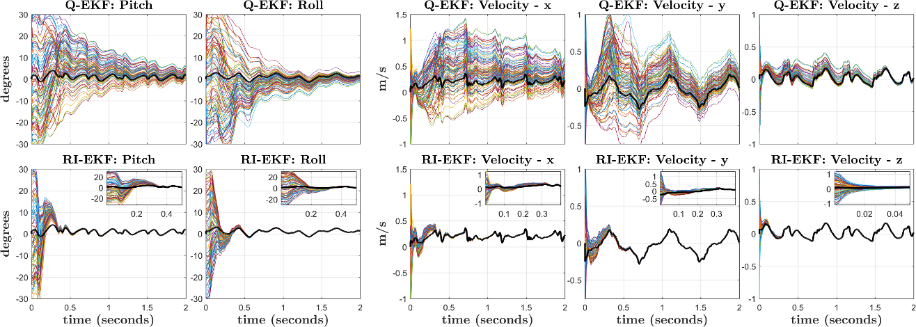
Refer to caption
Figure 8: An experiment was performed where an actual Cassie-series robot slowly walked forward at approximately 0.3m/sec0.3m0.3\leavevmode\nobreak\ \mathop{\mathrm{m}}/\sec. The noisy measurements came from the on-board IMU (VN-100) and the robot’s joint encoders. The quaternion-based extended Kalman filter (QEKF) and the proposed right-invariant extended Kalman filter (RIEKF) were run (off-line) 100 times using the same measurements, noise statistics, and initial covariance, but with random initial orientations and velocities. The black line represents the filter state estimates when initialized with a good estimate. The RIEKF (bottom row) converges considerably faster than the QEKF (top row) for all observable states. Zoomed-in plots of the RIEKF performance is provided in the top-right corner.

An experiment was performed where the robot walked forwards at approximately 0.3m/sec0.3m0.3\leavevmode\nobreak\ \mathop{\mathrm{m}}/\sec. The QEKF and the proposed RIEKF were run (off-line) 100 times using the same logged measurements, noise statistics, and initial covariance with random initial orientations and velocities. The noise statistics and initial covariance estimates are provided in Table 1. As with the simulation comparison presented in Section 6, the initial mean estimate for the Euler angles were uniformly sampled from 30deg30degree-30\deg to 30deg30degree30\deg and the initial mean estimate for velocities were sampled uniformly from 1.0m/sec1.0m-1.0\leavevmode\nobreak\ \mathop{\mathrm{m}}/\sec to 1.0m/sec1.0m1.0\leavevmode\nobreak\ \mathop{\mathrm{m}}/\sec. Bias estimation was turned on and the initial bias estimate was obtained from processing the IMU data when the robot was static. The pitch and roll estimates as well as the (body frame) velocity estimates for both filters are shown in Figure 8. The “ground truth” trajectory estimates (black lines) were computed by initializing each filter with a good state estimate at a time before the beginning of the plot (to allow for convergence). The initial orientation was obtained from the VectorNav-100’s onboard EKF and the initial velocity was obtained through kinematics alone.

The experimental results for comparing filter convergence matches those of the simulation. The proposed RIEKF converges faster and more reliably in all 100 runs than the QEKF; therefore, due to the convenience of initialization and reliability for tracking the developed RIEKF is the preferred observer.

When the state estimate is initialized close to the true value, the RIEKF and QEKF have similar performance (black lines), because the linearization of the error dynamics accurately reflects the underlying nonlinear dynamics. However, when the state estimate is far from the true value, the simulation and experimental results show that RIEKF consistently converges faster than the QEKF. The relatively poor performance of the QEKF is due to the error dynamics being linearized around the wrong operating point, in which case the linear system does not accurately reflect the nonlinear dynamics. In addition, when bias estimation is turned off, the invariant error dynamics of the RIEKF do not depend on the current state estimate. As a result, the linear error dynamics can be accurately used even when the current state estimate is far from its true value, leading to better performance over the QEKF. Although this theoretical advantage is lost when bias estimation is turned on, the experimental results (shown in Figure 8) indicate that the RIEKF still is the preferred observer due to less sensitivity to initialization.

9.2 Motion Capture Experiment

In order to verify the accuracy of the InEKF state estimate, we performed a motion capture experiment in the University of Michigan’s M-Air facility. This outdoor space is equipped with 18 Qualisys cameras that allows for position tracking. We had the Cassie robot walk untethered for 60sec6060\leavevmode\nobreak\ \sec along an approximately 15 mm\mathop{\mathrm{m}} path. A top-down view of the estimated trajectory is shown in Figure 9.
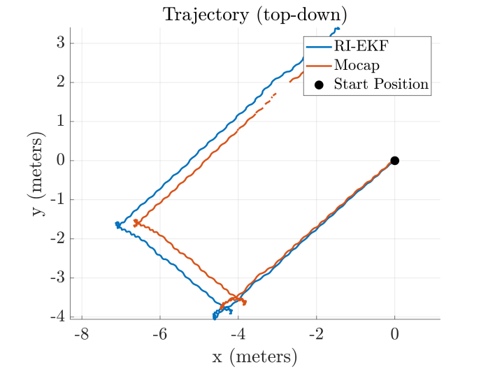
Refer to caption
Figure 9: Top-down view of the InEKF’s estimated trajectory for a motion capture experiment. The position drift is unobservable, however, the final drift is less than 5%percent55\% of the distance traveled.

Although there is noticeable drift due to the unobservability of the position and yaw, the final position error accounts for less than 5%percent55\% of the distance traveled. This drift error is due to a combination of sensor noise and imperfect modeling of the robot’s kinematics which may introduce biases to the forward kinematic measurements. The orientation, velocity, and position estimates along with their 3σ3𝜎3\sigma covariance hulls are shown in Figure 10. Due to the unobservability of the yaw angle, the velocity estimate is given in the body frame instead of the world frame. The orientation is plotted using exponential coordinates, exp(ϕ)=Rbold-italic-ϕR\exp(\boldsymbol{\phi})=\textbf{R}. Due to an inaccurate orientation estimate from the motion capture system, the “ground truth” for the orientation is given by the VectorNav-100, which runs a state-of-the-art QEKF that fuses angular velocity, linear acceleration, and magnetometer measurements to estimate orientation only.
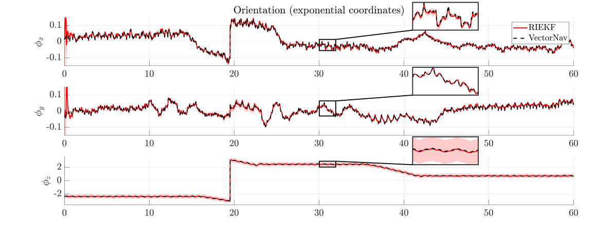
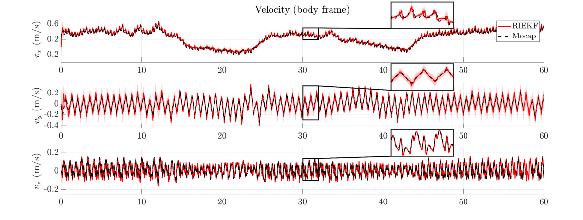
Refer to caption
Refer to caption
Refer to caption
Figure 10: Motion capture experiment conducted in the University of Michigan’s M-Air facility. The dashed black line represents ground truth, the solid red line is the right-invariant EKF estimate, and the red shaded area represents the 3σ3𝜎3\sigma covariance hull. The ground truth for position and velocity were obtained using 18 Qualisys cameras. Due to poor orientation estimates from the motion capture system, the “ground truth” for orientation was obtained from the VectorNav-100, which runs a highly accurate on-board QEKF. The orientation data is plotted using the exponential coordinates.

As expected, the error for all observable states remains small. The absolute position and the orientation about the gravity vector are unobservable, so some drift will occur for these states. While the drift is largely imperceptible for ϕzsubscriptbold-italic-ϕ𝑧\boldsymbol{\phi}_{z}, it is interesting to note that the covariance slowly grows over time due to this unobservability. More significant drift occurs on the absolute position states. This drift can be attributed to a combination of sensor noise, foot slip, and kinematic modeling errors.

In order to plot the 3σ3𝜎3\sigma covariance hull, the right-invariant error covariance needed to be converted to a covariance where the error is defined by Euclidean distance. Up to a first-order approximation, this mapping is done using:

[δϕtδvtδpt]=[𝚪11(ϕ¯t)00(v¯t)×I0(p¯t)×0I][𝝃tR𝝃tv𝝃tp],matrix𝛿subscriptbold-italic-ϕ𝑡𝛿subscriptv𝑡𝛿subscriptp𝑡matrixsuperscriptsubscript𝚪11subscript¯bold-italic-ϕ𝑡00subscriptsubscript¯v𝑡I0subscriptsubscript¯p𝑡0Imatrixsuperscriptsubscript𝝃𝑡𝑅superscriptsubscript𝝃𝑡𝑣superscriptsubscript𝝃𝑡𝑝\begin{bmatrix}\delta\boldsymbol{\phi}_{t}\\ \delta\textbf{v}_{t}\\ \delta\textbf{p}_{t}\end{bmatrix}=\begin{bmatrix}-\boldsymbol{\Gamma}_{1}^{-1}(\bar{\boldsymbol{\phi}}_{t})&\textbf{0}&\textbf{0}\\ \left(\bar{\textbf{v}}_{t}\right)_{\times}&-\textbf{I}&\textbf{0}\\ \left(\bar{\textbf{p}}_{t}\right)_{\times}&\textbf{0}&-\textbf{I}\\ \end{bmatrix}\begin{bmatrix}\boldsymbol{\xi}_{t}^{R}\\ \boldsymbol{\xi}_{t}^{v}\\ \boldsymbol{\xi}_{t}^{p}\\ \end{bmatrix}, (33)

where the “Euclidean orientation error” is defined as δϕtϕtϕ¯t𝛿subscriptbold-italic-ϕ𝑡subscriptbold-italic-ϕ𝑡subscript¯bold-italic-ϕ𝑡\delta\boldsymbol{\phi}_{t}\triangleq\boldsymbol{\phi}_{t}-\bar{\boldsymbol{\phi}}_{t}, and the velocity and position errors match the QEKF error states (21). The matrix 𝚪1(ϕ¯t)subscript𝚪1subscript¯bold-italic-ϕ𝑡\boldsymbol{\Gamma}_{1}(\bar{\boldsymbol{\phi}}_{t}) is known as the left Jacobian of SO(3)SO3\mathrm{SO}(3) and has an analytical form. Further explanation and the derivation of the above equation is given in Appendix C.

9.3 Long Odometry Experiment

In addition to providing accurate estimates of states vital for legged robot control (orientation and velocity), this InEKF can also provide reliable odometry for a higher-level mapping or SLAM system. To demonstrate the accuracy of long-term odometry, we had Cassie walk about 200m200m200\leavevmode\nobreak\ \mathop{\mathrm{m}} along a sidewalk around the University of Michigan’s Wave Field. In total, the walk took 7 minutes and 45 seconds. The estimated path from the InEKF overlaid onto Google Earth imagery is shown in Figure 11. A video of this experiment can be found at https://youtu.be/jRUltB_dMlo.
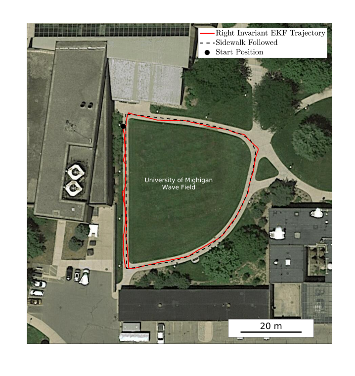
Refer to caption
Figure 11: Long outdoor odometry experiment where Cassie walked roughly 200m200m200\leavevmode\nobreak\ \mathop{\mathrm{m}} along a sidewalk over 7 minutes and 45 seconds.

Even though the absolute position is unobservable, the odometry estimate from the InEKF contains low enough drift to keep the estimate on the sidewalk for the duration of the experiment. The final position estimate is within a few meters of the true position, and the yaw drift is imperceptible. This odometry estimate is readily available, as it only depends on inertial, contact, and kinematic data, which barring sensor failure, always exist. It does not require the use of any vision systems that may be susceptible to changes in environment or lighting conditions.

9.4 LiDAR Mapping Application

One application for the InEKF odometry is the building of local maps of the environment. We equipped the Cassie-series robot with a new torso that houses a Velodyne VLP-32C LiDAR. With the filter running, we can project each received packet of point cloud data into the world frame based on the current state estimate. This point cloud data can then be accumulated to create a map of the environment. Figure 12 shows a few still frames from several LiDAR mapping experiments. Videos of these results can be viewed at https://youtu.be/pNyXsZ5zVZk and https://youtu.be/nbQTQw0gJ-k.
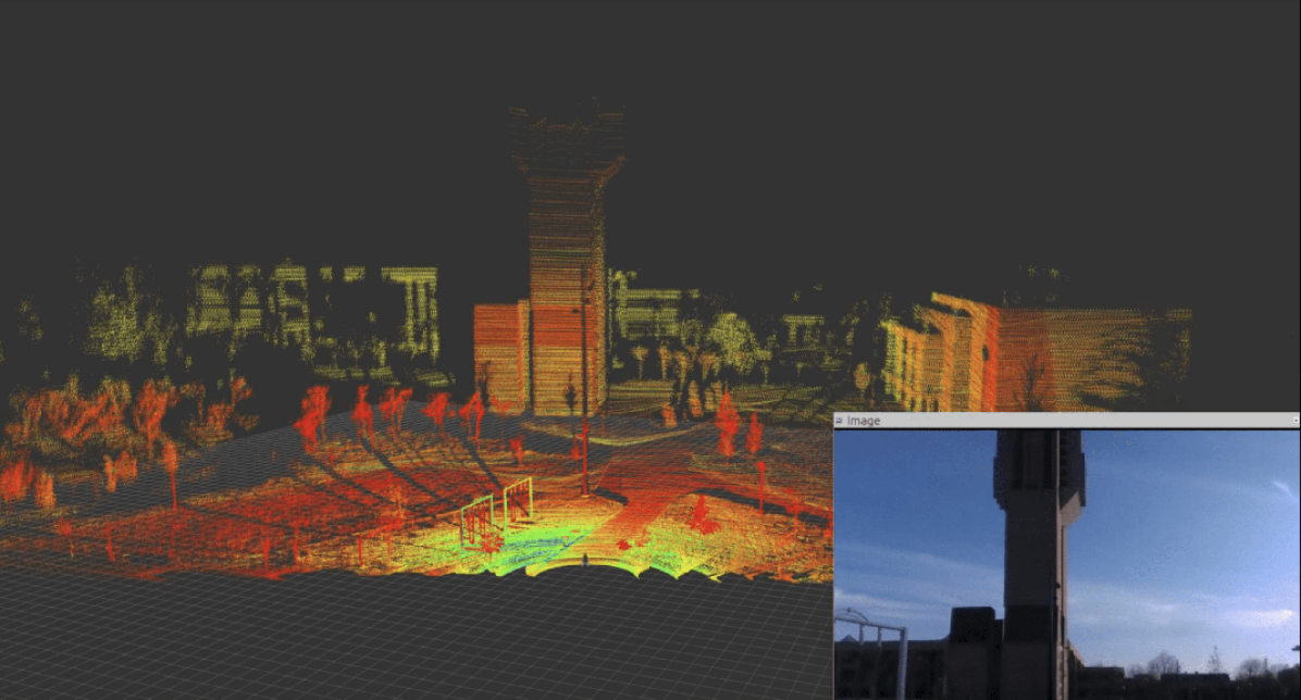
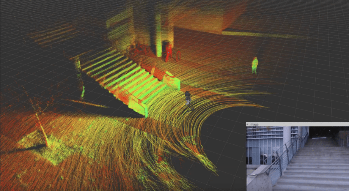
Refer to caption
(a) University of Michigan’s North Campus with the bell tower
Refer to caption
(b) Looking towards a staircase
Refer to caption
(c) Walking along a sidewalk
Refer to caption
(d) Inside the Bob and Betty Beyster Building
Figure 12: LiDAR maps created by transforming 10 seconds of point cloud data onto the pose trajectory estimated by the InEKF. The high frequency odometry estimate allows for motion compensation within a single scan of the LiDAR (10Hz); https://youtu.be/pNyXsZ5zVZk and https://youtu.be/nbQTQw0gJ-k.
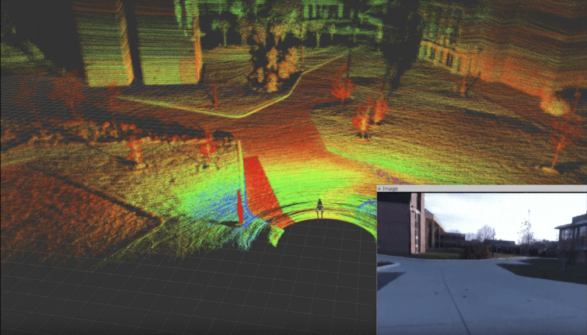
10 Alternative Left-Invariant Formulation

For the derivations in Sections 5-8, we were assuming the use of the right-invariant error. This choice was due to the forward kinematic measurement having the right-invariant observation form. However, it is possible to derive a left-invariant form of this filter, which may be more appropriate to use when dealing with left-invariant observations. For example, GPS measurements are left-invariant observations for the world-centric observer; see Section 12. Written explicitly, the left-invariant error is

𝜼tlXt1X¯t=[Rt𝖳R¯tRt𝖳(v¯tvt)Rt𝖳(p¯tpt)Rt𝖳(d¯tdt)01,310001,301001,3001].superscriptsubscript𝜼𝑡𝑙superscriptsubscriptX𝑡1subscript¯X𝑡matrixsuperscriptsubscriptR𝑡𝖳subscript¯R𝑡superscriptsubscriptR𝑡𝖳subscript¯v𝑡subscriptv𝑡superscriptsubscriptR𝑡𝖳subscript¯p𝑡subscriptp𝑡superscriptsubscriptR𝑡𝖳subscript¯d𝑡subscriptd𝑡subscript013100subscript013010subscript013001\begin{split}\boldsymbol{\eta}_{t}^{l}&\triangleq\textbf{X}_{t}^{-1}\bar{\textbf{X}}_{t}=\begin{bmatrix}\textbf{R}_{t}^{\mathsf{T}}\bar{\textbf{R}}_{t}&\textbf{R}_{t}^{\mathsf{T}}(\bar{\textbf{v}}_{t}-\textbf{v}_{t})&\textbf{R}_{t}^{\mathsf{T}}(\bar{\textbf{p}}_{t}-\textbf{p}_{t})&\textbf{R}_{t}^{\mathsf{T}}(\bar{\textbf{d}}_{t}-\textbf{d}_{t})\\ \textbf{0}_{1,3}&1&0&0\\ \textbf{0}_{1,3}&0&1&0\\ \textbf{0}_{1,3}&0&0&1\\ \end{bmatrix}.\end{split}

After carrying out the chain rule and making the first order approximation, 𝜼tl=exp(𝝃t)Id+𝝃tsuperscriptsubscript𝜼𝑡𝑙subscript𝝃𝑡subscriptI𝑑superscriptsubscript𝝃𝑡\boldsymbol{\eta}_{t}^{l}=\exp(\boldsymbol{\xi}_{t})\approx\textbf{{I}}_{d}+{\boldsymbol{\xi}_{t}}^{\wedge}, the individual terms of the left-invariant error dynamics become:

ddtRt𝖳R¯t((𝝎~t𝜻tg)×𝝃tR𝜻tg+wtg)×ddtRt𝖳(v¯tvt)(a~tb¯ta)×𝝃tR(𝝎~tb¯tg)×𝝃tv𝜻ta+wtaddtRt𝖳(p¯tpt)𝝃tv(𝝎~tb¯tg)×𝝃tpddtRt𝖳(d¯tdt)(𝝎~tb¯tg)×𝝃td+hR(𝜶~t)wtv.dd𝑡superscriptsubscriptR𝑡𝖳subscript¯R𝑡subscriptsubscriptsubscript~𝝎𝑡superscriptsubscript𝜻𝑡𝑔superscriptsubscript𝝃𝑡𝑅superscriptsubscript𝜻𝑡𝑔superscriptsubscriptw𝑡𝑔dd𝑡superscriptsubscriptR𝑡𝖳subscript¯v𝑡subscriptv𝑡subscriptsubscript~a𝑡superscriptsubscript¯b𝑡𝑎superscriptsubscript𝝃𝑡𝑅subscriptsubscript~𝝎𝑡superscriptsubscript¯b𝑡𝑔superscriptsubscript𝝃𝑡𝑣superscriptsubscript𝜻𝑡𝑎superscriptsubscriptw𝑡𝑎dd𝑡superscriptsubscriptR𝑡𝖳subscript¯p𝑡subscriptp𝑡superscriptsubscript𝝃𝑡𝑣subscriptsubscript~𝝎𝑡superscriptsubscript¯b𝑡𝑔superscriptsubscript𝝃𝑡𝑝dd𝑡superscriptsubscriptR𝑡𝖳subscript¯d𝑡subscriptd𝑡subscriptsubscript~𝝎𝑡superscriptsubscript¯b𝑡𝑔superscriptsubscript𝝃𝑡𝑑subscripth𝑅subscript~𝜶𝑡superscriptsubscriptw𝑡𝑣\begin{split}\dfrac{\mathrm{d}}{\mathrm{d}t}\textbf{R}_{t}^{\mathsf{T}}\bar{\textbf{R}}_{t}&\approx\left(-\left(\tilde{\boldsymbol{\omega}}_{t}-\boldsymbol{\zeta}_{t}^{g}\right)_{\times}\boldsymbol{\xi}_{t}^{R}-\boldsymbol{\zeta}_{t}^{g}+\textbf{w}_{t}^{g}\right)_{\times}\\ \dfrac{\mathrm{d}}{\mathrm{d}t}\textbf{R}_{t}^{\mathsf{T}}(\bar{\textbf{v}}_{t}-\textbf{v}_{t})&\approx-\left(\tilde{\textbf{a}}_{t}-\bar{\textbf{b}}_{t}^{a}\right)_{\times}\boldsymbol{\xi}_{t}^{R}-\left(\tilde{\boldsymbol{\omega}}_{t}-\bar{\textbf{b}}_{t}^{g}\right)_{\times}\boldsymbol{\xi}_{t}^{v}-\boldsymbol{\zeta}_{t}^{a}+\textbf{w}_{t}^{a}\\ \dfrac{\mathrm{d}}{\mathrm{d}t}\textbf{R}_{t}^{\mathsf{T}}(\bar{\textbf{p}}_{t}-\textbf{p}_{t})&\approx\boldsymbol{\xi}_{t}^{v}-\left(\tilde{\boldsymbol{\omega}}_{t}-\bar{\textbf{b}}_{t}^{g}\right)_{\times}\boldsymbol{\xi}_{t}^{p}\\ \dfrac{\mathrm{d}}{\mathrm{d}t}\textbf{R}_{t}^{\mathsf{T}}(\bar{\textbf{d}}_{t}-\textbf{d}_{t})&\approx-\left(\tilde{\boldsymbol{\omega}}_{t}-\bar{\textbf{b}}_{t}^{g}\right)_{\times}\boldsymbol{\xi}_{t}^{d}+\;\textit{{h}}_{R}(\tilde{\boldsymbol{\alpha}}_{t})\textbf{w}_{t}^{v}.\\ \end{split}

Using these results, the log-linear left-invariant dynamics can be expressed using the following linear system

ddt𝝃t=At𝝃t+wtddtPt=AtPt+PtAt𝖳+Q¯t,dd𝑡subscript𝝃𝑡subscriptA𝑡subscript𝝃𝑡subscriptw𝑡dd𝑡subscriptP𝑡subscriptA𝑡subscriptP𝑡subscriptP𝑡superscriptsubscriptA𝑡𝖳subscript¯Q𝑡\begin{split}\dfrac{\mathrm{d}}{\mathrm{d}t}\boldsymbol{\xi}_{t}&=\textbf{A}_{t}\boldsymbol{\xi}_{t}+\textbf{w}_{t}\\ \implies\dfrac{\mathrm{d}}{\mathrm{d}t}\textbf{P}_{t}&=\textbf{A}_{t}\textbf{P}_{t}+\textbf{P}_{t}\textbf{A}_{t}^{\mathsf{T}}+\bar{\textbf{Q}}_{t},\end{split}

where the dynamics and noise matrices are

Atl=[(𝝎¯t)×000I0(a¯t)×(𝝎¯t)×000I0I(𝝎¯t)×000000(𝝎¯t)×00000000000000]Q¯t=Cov(wt).superscriptsubscriptA𝑡𝑙matrixsubscriptsubscript¯𝝎𝑡000I0subscriptsubscript¯a𝑡subscriptsubscript¯𝝎𝑡000I0Isubscriptsubscript¯𝝎𝑡000000subscriptsubscript¯𝝎𝑡00000000000000subscript¯Q𝑡Covsubscriptw𝑡\begin{split}\textbf{A}_{t}^{l}&=\begin{bmatrix}-\left(\bar{\boldsymbol{\omega}}_{t}\right)_{\times}&\textbf{0}&\textbf{0}&\textbf{0}&-\textbf{I}&\textbf{0}\\ -\left(\bar{\textbf{a}}_{t}\right)_{\times}&-\left(\bar{\boldsymbol{\omega}}_{t}\right)_{\times}&\textbf{0}&\textbf{0}&\textbf{0}&-\textbf{I}\\ \textbf{0}&\textbf{I}&-\left(\bar{\boldsymbol{\omega}}_{t}\right)_{\times}&\textbf{0}&\textbf{0}&\textbf{0}\\ \textbf{0}&\textbf{0}&\textbf{0}&-\left(\bar{\boldsymbol{\omega}}_{t}\right)_{\times}&\textbf{0}&\textbf{0}\\ \textbf{0}&\textbf{0}&\textbf{0}&\textbf{0}&\textbf{0}&\textbf{0}\\ \textbf{0}&\textbf{0}&\textbf{0}&\textbf{0}&\textbf{0}&\textbf{0}\\ \end{bmatrix}\\ \bar{\textbf{Q}}_{t}&=\text{Cov}(\textbf{w}_{t}).\end{split} (34)

Similar to the right-invariant case, the dynamics only depend on the state through the IMU bias. When a left-invariant observation comes in, the state estimate is corrected using

(X¯t+,𝜽t+)=(X¯texp(Kt𝝃𝚷X¯t1Yt),𝜽¯t+Kt𝜻𝚷X¯t1Yt),superscriptsubscript¯X𝑡superscriptsubscript𝜽𝑡subscript¯X𝑡superscriptsubscriptK𝑡𝝃𝚷superscriptsubscript¯X𝑡1subscriptY𝑡subscript¯𝜽𝑡superscriptsubscriptK𝑡𝜻𝚷superscriptsubscript¯X𝑡1subscriptY𝑡\left(\bar{\textbf{X}}_{t}^{+},\boldsymbol{\theta}_{t}^{+}\right)=\left(\bar{\textbf{X}}_{t}\exp\left(\textbf{K}_{t}^{\boldsymbol{\xi}}\boldsymbol{\Pi}\bar{\textbf{X}}_{t}^{-1}\textbf{Y}_{t}\right)\,,\;\;\bar{\boldsymbol{\theta}}_{t}+\textbf{K}_{t}^{\boldsymbol{\zeta}}\boldsymbol{\Pi}\bar{\textbf{X}}_{t}^{-1}\textbf{Y}_{t}\right), (35)

where the exponential map is now multiplied on the right side [10].

10.1 Switching Between Left and Right-Invariant Errors

Because forward kinematic measurements have the right invariant observation form, the innovation equations are only autonomous when the right invariant error is used. Fortunately, it is possible to switch between the left and right error forms through the use of the adjoint map.

𝜼tr=X¯tXt1=X¯t𝜼tlX¯t1exp(𝝃tr)=X¯texp(𝝃tl)X¯t1=exp(AdX¯t𝝃tl)𝝃tr=AdX¯t𝝃tlsuperscriptsubscript𝜼𝑡𝑟subscript¯X𝑡superscriptsubscriptX𝑡1subscript¯X𝑡superscriptsubscript𝜼𝑡𝑙superscriptsubscript¯X𝑡1superscriptsubscript𝝃𝑡𝑟subscript¯X𝑡superscriptsubscript𝝃𝑡𝑙superscriptsubscript¯X𝑡1subscriptAdsubscript¯X𝑡superscriptsubscript𝝃𝑡𝑙superscriptsubscript𝝃𝑡𝑟subscriptAdsubscript¯X𝑡superscriptsubscript𝝃𝑡𝑙\begin{split}\boldsymbol{\eta}_{t}^{r}&=\bar{\textbf{X}}_{t}\textbf{X}_{t}^{-1}=\bar{\textbf{X}}_{t}\boldsymbol{\eta}_{t}^{l}\bar{\textbf{X}}_{t}^{-1}\\ \implies\exp(\boldsymbol{\xi}_{t}^{r})&=\bar{\textbf{X}}_{t}\exp(\boldsymbol{\xi}_{t}^{l})\bar{\textbf{X}}_{t}^{-1}=\exp(\mathrm{Ad}_{\bar{\textbf{X}}_{t}}\boldsymbol{\xi}_{t}^{l})\\ \implies\boldsymbol{\xi}_{t}^{r}&=\mathrm{Ad}_{\bar{\textbf{X}}_{t}}\boldsymbol{\xi}_{t}^{l}\\ \end{split}

This transformation is exact, which means that we can easily switch between the covariance of the left and right invariant errors using

Ptr=AdX¯tPtlAdX¯t𝖳.superscriptsubscriptP𝑡𝑟subscriptAdsubscript¯X𝑡superscriptsubscriptP𝑡𝑙superscriptsubscriptAdsubscript¯X𝑡𝖳\textbf{P}_{t}^{r}=\mathrm{Ad}_{\bar{\textbf{X}}_{t}}\,\textbf{P}_{t}^{l}\,\mathrm{Ad}_{\bar{\textbf{X}}_{t}}^{\mathsf{T}}. (36)

Therefore, when handling a right-invariant observation, we can map the propagated left-invariant covariance to the right-invariant covariance temporarily, apply the right-invariant update equations (29), then map the corrected covariance back to the left-invariant form.

It is also possible to compute the log-linear left-invariant dynamics starting from the right-invariant form. Substituting (36) into the (right-invariant) covariance propagation equation (13) and solving for the left-invariant covariance yields

ddtPtl=(AdX¯t1AtrAdX¯tAdX¯t1ddt(AdX¯t))Ptl+Ptl(AdX¯t𝖳Atr𝖳AdX¯t1𝖳ddt(AdX¯t𝖳)AdX¯t1𝖳)+AdX¯t1Q¯trAdX¯t1𝖳.dd𝑡superscriptsubscriptP𝑡𝑙subscriptAdsuperscriptsubscript¯X𝑡1superscriptsubscriptA𝑡𝑟subscriptAdsubscript¯X𝑡subscriptAdsuperscriptsubscript¯X𝑡1dd𝑡subscriptAdsubscript¯X𝑡superscriptsubscriptP𝑡𝑙superscriptsubscriptP𝑡𝑙superscriptsubscriptAdsubscript¯X𝑡𝖳superscriptsubscriptA𝑡𝑟𝖳superscriptsubscriptAdsuperscriptsubscript¯X𝑡1𝖳dd𝑡superscriptsubscriptAdsubscript¯X𝑡𝖳superscriptsubscriptAdsuperscriptsubscript¯X𝑡1𝖳subscriptAdsuperscriptsubscript¯X𝑡1subscriptsuperscript¯Q𝑟𝑡superscriptsubscriptAdsuperscriptsubscript¯X𝑡1𝖳\begin{split}\dfrac{\mathrm{d}}{\mathrm{d}t}\textbf{P}_{t}^{l}=&\left(\mathrm{Ad}_{\bar{\textbf{X}}_{t}^{-1}}\textbf{A}_{t}^{r}\mathrm{Ad}_{\bar{\textbf{X}}_{t}}-\mathrm{Ad}_{\bar{\textbf{X}}_{t}^{-1}}\dfrac{\mathrm{d}}{\mathrm{d}t}\left(\mathrm{Ad}_{\bar{\textbf{X}}_{t}}\right)\right)\textbf{P}_{t}^{l}\\ &+\textbf{P}_{t}^{l}\left(\mathrm{Ad}_{\bar{\textbf{X}}_{t}}^{\mathsf{T}}\textbf{A}_{t}^{r\mathsf{T}}\mathrm{Ad}_{\bar{\textbf{X}}_{t}^{-1}}^{\mathsf{T}}-\dfrac{\mathrm{d}}{\mathrm{d}t}\left(\mathrm{Ad}_{\bar{\textbf{X}}_{t}}^{\mathsf{T}}\right)\mathrm{Ad}_{\bar{\textbf{X}}_{t}^{-1}}^{\mathsf{T}}\right)\\ &+\mathrm{Ad}_{\bar{\textbf{X}}_{t}^{-1}}\bar{\textbf{Q}}^{r}_{t}\mathrm{Ad}_{\bar{\textbf{X}}_{t}^{-1}}^{\mathsf{T}}.\end{split}

Therefore, we learn that the right and left dynamics and noise matrices are related by the following expressions

AtlAdX¯t1AtrAdX¯tAdX¯t1ddt(AdX¯t)Q¯tlAdX¯t1Q¯trAdX¯t1𝖳.superscriptsubscriptA𝑡𝑙subscriptAdsuperscriptsubscript¯X𝑡1superscriptsubscriptA𝑡𝑟subscriptAdsubscript¯X𝑡subscriptAdsuperscriptsubscript¯X𝑡1dd𝑡subscriptAdsubscript¯X𝑡subscriptsuperscript¯Q𝑙𝑡subscriptAdsuperscriptsubscript¯X𝑡1subscriptsuperscript¯Q𝑟𝑡superscriptsubscriptAdsuperscriptsubscript¯X𝑡1𝖳\begin{split}\textbf{A}_{t}^{l}&\triangleq\mathrm{Ad}_{\bar{\textbf{X}}_{t}^{-1}}\textbf{A}_{t}^{r}\mathrm{Ad}_{\bar{\textbf{X}}_{t}}-\mathrm{Ad}_{\bar{\textbf{X}}_{t}^{-1}}\dfrac{\mathrm{d}}{\mathrm{d}t}\left(\mathrm{Ad}_{\bar{\textbf{X}}_{t}}\right)\\ \bar{\textbf{Q}}^{l}_{t}&\triangleq\mathrm{Ad}_{\bar{\textbf{X}}_{t}^{-1}}\bar{\textbf{Q}}^{r}_{t}\mathrm{Ad}_{\bar{\textbf{X}}_{t}^{-1}}^{\mathsf{T}}.\end{split} (37)
Remark 6.

Intuitively, the left-invariant error represents an error measured in the body frame of the robot, while the right-invariant error represents an error measured in the world or spatial frame. The frame of measurement dictates whether the exponential map appears on the right or left in the update equations. The error can be moved between these two frames using the adjoint map of the Lie group.

10.2 Adding New Contact Points

The process for removing a contact point from the state (marginalization) is identical to the right-invariant error case, described in Section 8.1. Likewise, when a new contact is detected, the state can be augmented using the same kinematics relation (31) as before. However, due to the change in error variable, the process for augmenting the covariance will be different.

In order to compute the new covariance, we need to look at the left-invariant error,

𝜼td=Rt𝖳(d¯tdt)=Rt𝖳(p¯t+R¯thp(𝜶~t))Rt𝖳(pt+Rthp(𝜶~twtα))𝜼tp+𝜼tRhp(𝜶~t)hp(𝜶~t)+Jp(𝜶~t)wtα𝝃td𝝃tp(hp(𝜶~t))×𝝃tR+Jp(𝜶~t)wtα.superscriptsubscript𝜼𝑡𝑑superscriptsubscriptR𝑡𝖳subscript¯d𝑡subscriptd𝑡superscriptsubscriptR𝑡𝖳subscript¯p𝑡subscript¯R𝑡subscripth𝑝subscript~𝜶𝑡superscriptsubscriptR𝑡𝖳subscriptp𝑡subscriptR𝑡subscripth𝑝subscript~𝜶𝑡superscriptsubscriptw𝑡𝛼superscriptsubscript𝜼𝑡𝑝superscriptsubscript𝜼𝑡𝑅subscripth𝑝subscript~𝜶𝑡subscripth𝑝subscript~𝜶𝑡subscriptJ𝑝subscript~𝜶𝑡superscriptsubscriptw𝑡𝛼superscriptsubscript𝝃𝑡𝑑superscriptsubscript𝝃𝑡𝑝subscriptsubscripth𝑝subscript~𝜶𝑡superscriptsubscript𝝃𝑡𝑅subscriptJ𝑝subscript~𝜶𝑡superscriptsubscriptw𝑡𝛼\begin{split}\boldsymbol{\eta}_{t}^{d}&=\textbf{R}_{t}^{\mathsf{T}}(\bar{\textbf{d}}_{t}-\textbf{d}_{t})\\ &=\textbf{R}_{t}^{\mathsf{T}}\left(\bar{\textbf{p}}_{t}+\bar{\textbf{R}}_{t}\;\textit{{h}}_{p}(\tilde{\boldsymbol{\alpha}}_{t})\right)-\textbf{R}_{t}^{\mathsf{T}}\left(\textbf{p}_{t}+\textbf{R}_{t}\;\textit{{h}}_{p}(\tilde{\boldsymbol{\alpha}}_{t}-\textbf{w}_{t}^{\alpha})\right)\\ &\approx\boldsymbol{\eta}_{t}^{p}+\boldsymbol{\eta}_{t}^{R}\;\textit{{h}}_{p}(\tilde{\boldsymbol{\alpha}}_{t})-\;\textit{{h}}_{p}(\tilde{\boldsymbol{\alpha}}_{t})+\textbf{J}_{p}(\tilde{\boldsymbol{\alpha}}_{t})\textbf{w}_{t}^{\alpha}\\ \implies\boldsymbol{\xi}_{t}^{d}&\approx\boldsymbol{\xi}_{t}^{p}-\left(\;\textit{{h}}_{p}(\tilde{\boldsymbol{\alpha}}_{t})\right)_{\times}\boldsymbol{\xi}_{t}^{R}+\textbf{J}_{p}(\tilde{\boldsymbol{\alpha}}_{t})\textbf{w}_{t}^{\alpha}.\end{split}

Therefore, covariance augmentation can be done using the following linear map,

[𝝃tR𝝃tv𝝃tp𝝃td]=[I000I000I(hp(𝜶~t))×0I][𝝃tR𝝃tv𝝃tp]+[000Jp(𝜶~t)]wtα𝝃tnewFt𝝃t+GtwtαPtnew=FtPtFt𝖳+GtCov(wtα)Gt𝖳.matrixsuperscriptsubscript𝝃𝑡𝑅superscriptsubscript𝝃𝑡𝑣superscriptsubscript𝝃𝑡𝑝superscriptsubscript𝝃𝑡𝑑matrixI000I000Isubscriptsubscripth𝑝subscript~𝜶𝑡0Imatrixsuperscriptsubscript𝝃𝑡𝑅superscriptsubscript𝝃𝑡𝑣superscriptsubscript𝝃𝑡𝑝matrix000subscriptJ𝑝subscript~𝜶𝑡superscriptsubscriptw𝑡𝛼superscriptsubscript𝝃𝑡newsubscriptF𝑡subscript𝝃𝑡subscriptG𝑡superscriptsubscriptw𝑡𝛼superscriptsubscriptP𝑡newsubscriptF𝑡subscriptP𝑡superscriptsubscriptF𝑡𝖳subscriptG𝑡Covsuperscriptsubscriptw𝑡𝛼superscriptsubscriptG𝑡𝖳\begin{split}\begin{bmatrix}\boldsymbol{\xi}_{t}^{R}\\ \boldsymbol{\xi}_{t}^{v}\\ \boldsymbol{\xi}_{t}^{p}\\ \boldsymbol{\xi}_{t}^{d}\\ \end{bmatrix}&=\begin{bmatrix}\textbf{I}&\textbf{0}&\textbf{0}\\ \textbf{0}&\textbf{I}&\textbf{0}\\ \textbf{0}&\textbf{0}&\textbf{I}\\ \left(-\;\textit{{h}}_{p}(\tilde{\boldsymbol{\alpha}}_{t})\right)_{\times}&\textbf{0}&\textbf{I}\\ \end{bmatrix}\begin{bmatrix}\boldsymbol{\xi}_{t}^{R}\\ \boldsymbol{\xi}_{t}^{v}\\ \boldsymbol{\xi}_{t}^{p}\\ \end{bmatrix}+\begin{bmatrix}\textbf{0}\\ \textbf{0}\\ \textbf{0}\\ \textbf{J}_{p}(\tilde{\boldsymbol{\alpha}}_{t})\\ \end{bmatrix}\textbf{w}_{t}^{\alpha}\\ \boldsymbol{\xi}_{t}^{\mathrm{new}}&\triangleq\textbf{F}_{t}\,\boldsymbol{\xi}_{t}+\textbf{G}_{t}\textbf{w}_{t}^{\alpha}\\ \implies\textbf{P}_{t}^{\mathrm{new}}&=\textbf{F}_{t}\,\textbf{P}_{t}\,\textbf{F}_{t}^{\mathsf{T}}+\textbf{G}_{t}\,\text{Cov}(\textbf{w}_{t}^{\alpha})\,\textbf{G}_{t}^{\mathsf{T}}.\end{split} (38)

11 Robo-centric Estimator

In this section, we derive a “robot-centric” version of the contact-aided InEKF where the estimated state is measured in the robot’s base (IMU) frame. When switching to a robot-centric model, the forward kinematics measurements take the left-invariant observation form. In addition, the left/right-invariant error dynamics equations are identical to the world-centric form, albeit swapped. The right-invariant error dynamics for the world-centric estimator are equivalent to the left-invariant error dynamics for the robo-centric estimator.

The properties of this filter are identical to the RIEKF derived in Section 5. However, in some cases this filter may be preferred as it directly estimates states that are useful for controlling a legged robot (namely the velocity measured in the body frame).

11.1 State and Dynamics

We are interested in estimating the same states as before, though measured in the robot’s body frame. Again, the state variables can form a matrix Lie group, 𝒢𝒢\mathcal{G}. Specifically, for N𝑁N contact points, XtSEN+2(3)subscriptX𝑡subscriptSE𝑁23\textbf{X}_{t}\in\mathrm{SE}_{N+2}(3) can be represented by the following matrix (which is simply the inverse of the world-centric state)555The negative sign on body velocity appears when inverting the world-centric state; vBB=RWB𝖳vBWsubscriptsubscriptvBBsuperscriptsubscriptRWB𝖳subscriptsubscriptvBW-{}_{\text{B}}\textbf{v}_{\text{B}}=-\textbf{R}_{\text{WB}}^{\mathsf{T}}\,{}_{\text{W}}\textbf{v}_{\text{B}}. This sign is removed on the position vectors by swapping the start and end points, pBWB=RWB𝖳pWBBsubscriptsubscriptpBWBsuperscriptsubscriptRWB𝖳subscriptsubscriptpWBB{}_{\text{B}}\textbf{p}_{\text{BW}}=-\textbf{R}_{\text{WB}}^{\mathsf{T}}\,{}_{\text{B}}\textbf{p}_{\text{WB}}.:

Xtredefine[RBW(t)vBB(t)pBWB(t)pC1WB(t)pCNWB(t)01×3100001×3010001×3001001×30001]redefinesubscriptX𝑡matrixsubscriptRBW𝑡subscriptsubscriptvBB𝑡subscriptsubscriptpBWB𝑡subscriptsubscriptpsubscriptC1WB𝑡subscriptsubscriptpsubscriptC𝑁WB𝑡subscript0131000subscript0130100subscript0130010subscript0130001\textbf{X}_{t}\leavevmode\nobreak\ \mathrel{\overset{\makebox[0.0pt]{\mbox{\tiny redefine}}}{\triangleq}}\leavevmode\nobreak\ \begin{bmatrix}\textbf{R}_{\text{BW}}(t)&-{}_{\text{B}}\textbf{v}_{\text{B}}(t)&{}_{\text{B}}\textbf{p}_{\text{BW}}(t)&{}_{\text{B}}\textbf{p}_{\text{C}_{1}\text{W}}(t)&\cdots&{}_{\text{B}}\textbf{p}_{\text{C}_{N}\text{W}}(t)\\ \textbf{0}_{1\times 3}&1&0&0&\cdots&0\\ \textbf{0}_{1\times 3}&0&1&0&\cdots&0\\ \textbf{0}_{1\times 3}&0&0&1&\cdots&0\\ \vdots&\vdots&\vdots&\vdots&\ddots&\vdots\\ \textbf{0}_{1\times 3}&0&0&0&\cdots&1\\ \end{bmatrix}

Without loss of generality, assume a single contact point. Furthermore, for the sake of readability, we redefine our shorthand notation to be body-centric states,

Xtredefine[Rtvtptdt01×310001×301001×3001].subscriptX𝑡redefinematrixsubscriptR𝑡subscriptv𝑡subscriptp𝑡subscriptd𝑡subscript013100subscript013010subscript013001\textbf{X}_{t}\leavevmode\nobreak\ \leavevmode\nobreak\ \mathrel{\overset{\makebox[0.0pt]{\mbox{\tiny redefine}}}{\triangleq}}\leavevmode\nobreak\ \leavevmode\nobreak\ \begin{bmatrix}\textbf{R}_{t}&\textbf{v}_{t}&\textbf{p}_{t}&\textbf{d}_{t}\\ \textbf{0}_{1\times 3}&1&0&0\\ \textbf{0}_{1\times 3}&0&1&0\\ \textbf{0}_{1\times 3}&0&0&1\\ \end{bmatrix}. (39)

Using the bias corrected IMU measurements, the individual terms of the new robot-centric system dynamics can be derived as [16]

ddtRt=(𝝎¯twtg)×Rtddtvt=(a¯twta)Rtg(𝝎¯twtg)×vtddtpt=vt(𝝎¯twtg)×ptddtdt=(𝝎¯twtg)×dthR(𝜶~t)wtv.dd𝑡subscriptR𝑡subscriptsubscript¯𝝎𝑡superscriptsubscriptw𝑡𝑔subscriptR𝑡dd𝑡subscriptv𝑡subscript¯a𝑡superscriptsubscriptw𝑡𝑎subscriptR𝑡gsubscriptsubscript¯𝝎𝑡superscriptsubscriptw𝑡𝑔subscriptv𝑡dd𝑡subscriptp𝑡subscriptv𝑡subscriptsubscript¯𝝎𝑡superscriptsubscriptw𝑡𝑔subscriptp𝑡dd𝑡subscriptd𝑡subscriptsubscript¯𝝎𝑡superscriptsubscriptw𝑡𝑔subscriptd𝑡subscripth𝑅subscript~𝜶𝑡superscriptsubscriptw𝑡𝑣\begin{split}\dfrac{\mathrm{d}}{\mathrm{d}t}\textbf{R}_{t}&=-\left(\bar{\boldsymbol{\omega}}_{t}-\textbf{w}_{t}^{g}\right)_{\times}\textbf{R}_{t}\\ \dfrac{\mathrm{d}}{\mathrm{d}t}\textbf{v}_{t}&=-(\bar{\textbf{a}}_{t}-\textbf{w}_{t}^{a})-\textbf{R}_{t}\,\textbf{g}-\left(\bar{\boldsymbol{\omega}}_{t}-\textbf{w}_{t}^{g}\right)_{\times}\textbf{v}_{t}\\ \dfrac{\mathrm{d}}{\mathrm{d}t}\textbf{p}_{t}&=\textbf{v}_{t}-\left(\bar{\boldsymbol{\omega}}_{t}-\textbf{w}_{t}^{g}\right)_{\times}\textbf{p}_{t}\\ \dfrac{\mathrm{d}}{\mathrm{d}t}\textbf{d}_{t}&=-\left(\bar{\boldsymbol{\omega}}_{t}-\textbf{w}_{t}^{g}\right)_{\times}\textbf{d}_{t}-\;\textit{{h}}_{R}(\tilde{\boldsymbol{\alpha}}_{t})\textbf{w}_{t}^{v}.\end{split} (40)

Written in matrix form, this becomes

ddtXt=[(𝝎¯t)×Rta¯tRtg(𝝎~t)×vtvt(𝝎~t)×pt(𝝎¯t)×dt01,300001,300001,3000][(wtg)×wta03,1hR(𝜶~t)wtv01,300001,300001,3000][Rtvtptdt01,310001,301001,3001]fu(Xt,𝜽t)wtXtdd𝑡subscriptX𝑡matrixsubscriptsubscript¯𝝎𝑡subscriptR𝑡subscript¯a𝑡subscriptR𝑡gsubscriptsubscript~𝝎𝑡subscriptv𝑡subscriptv𝑡subscriptsubscript~𝝎𝑡subscriptp𝑡subscriptsubscript¯𝝎𝑡subscriptd𝑡subscript013000subscript013000subscript013000matrixsubscriptsuperscriptsubscriptw𝑡𝑔superscriptsubscriptw𝑡𝑎subscript031subscripth𝑅subscript~𝜶𝑡superscriptsubscriptw𝑡𝑣subscript013000subscript013000subscript013000matrixsubscriptR𝑡subscriptv𝑡subscriptp𝑡subscriptd𝑡subscript013100subscript013010subscript013001subscript𝑓𝑢subscriptX𝑡subscript𝜽𝑡superscriptsubscriptw𝑡subscriptX𝑡\begin{split}\dfrac{\mathrm{d}}{\mathrm{d}t}\textbf{X}_{t}&=\begin{bmatrix}-\left(\bar{\boldsymbol{\omega}}_{t}\right)_{\times}\textbf{R}_{t}&-\bar{\textbf{a}}_{t}-\textbf{R}_{t}\textbf{g}-\left(\tilde{\boldsymbol{\omega}}_{t}\right)_{\times}\textbf{v}_{t}&\textbf{v}_{t}-\left(\tilde{\boldsymbol{\omega}}_{t}\right)_{\times}\textbf{p}_{t}&-\left(\bar{\boldsymbol{\omega}}_{t}\right)_{\times}\textbf{d}_{t}\\ \textbf{0}_{1,3}&0&0&0\\ \textbf{0}_{1,3}&0&0&0\\ \textbf{0}_{1,3}&0&0&0\\ \end{bmatrix}-\begin{bmatrix}\left(\textbf{w}_{t}^{g}\right)_{\times}&\textbf{w}_{t}^{a}&\textbf{0}_{3,1}&\;\textit{{h}}_{R}(\tilde{\boldsymbol{\alpha}}_{t})\textbf{w}_{t}^{v}\\ \textbf{0}_{1,3}&0&0&0\\ \textbf{0}_{1,3}&0&0&0\\ \textbf{0}_{1,3}&0&0&0\\ \end{bmatrix}\begin{bmatrix}\textbf{R}_{t}&\textbf{v}_{t}&\textbf{p}_{t}&\textbf{d}_{t}\\ \textbf{0}_{1,3}&1&0&0\\ \textbf{0}_{1,3}&0&1&0\\ \textbf{0}_{1,3}&0&0&1\\ \end{bmatrix}\\ &\triangleq f_{u}(\textbf{X}_{t},\boldsymbol{\theta}_{t})-{\textbf{w}_{t}}^{\wedge}\textbf{X}_{t}\end{split}

(41)

with wtvec(wtg,wta,03,1,hR(𝜶~t)wtv)subscriptw𝑡vecsuperscriptsubscriptw𝑡𝑔superscriptsubscriptw𝑡𝑎subscript031subscripth𝑅subscript~𝜶𝑡superscriptsubscriptw𝑡𝑣\textbf{w}_{t}\triangleq\mathrm{vec}(\textbf{w}_{t}^{g},\,\textbf{w}_{t}^{a},\,\textbf{0}_{3,1},\;\textit{{h}}_{R}(\tilde{\boldsymbol{\alpha}}_{t})\textbf{w}_{t}^{v}). The deterministic dynamics function fu()subscript𝑓𝑢f_{u}(\cdot) can be shown to satisfy the group affine property (2). Therefore, the left (and right) invariant error dynamics depends solely on the invariant error.

We can derive the log-linear dynamics matrices for the body-centric estimator following a similar derivation process to the world-centric version in Section 5. In fact, without IMU bias, the linearization of the left-invariant dynamics for the body-centric estimator is the same as the right-invariant dynamics for the world-centric estimator;

Atl(body-centric)=Atr(world-centric)Atr(body-centric)=Atl(world-centric).superscriptsubscriptA𝑡𝑙(body-centric)superscriptsubscriptA𝑡𝑟(world-centric)superscriptsubscriptA𝑡𝑟(body-centric)superscriptsubscriptA𝑡𝑙(world-centric)\begin{split}\textbf{A}_{t}^{l}\;\textit{(body-centric)}&=\textbf{A}_{t}^{r}\;\textit{(world-centric)}\\ \textbf{A}_{t}^{r}\;\textit{(body-centric)}&=\textbf{A}_{t}^{l}\;\textit{(world-centric)}.\\ \end{split} (42)

When IMU bias is included, the above relation still holds, though with the bias terms negated666If definition of bias error is negated, even these terms would remain the same.. The noise covariance matrices for the body-centric left/right-invariant propagation models are given by:

Q¯tl=[AdX¯t1015,606,15I6]Cov(wt)[AdX¯t1015,606,15I6]𝖳Q¯tr=Cov(wt),subscriptsuperscript¯Q𝑙𝑡matrixsubscriptAdsuperscriptsubscript¯X𝑡1subscript0156subscript0615subscriptI6Covsubscriptw𝑡superscriptmatrixsubscriptAdsuperscriptsubscript¯X𝑡1subscript0156subscript0615subscriptI6𝖳subscriptsuperscript¯Q𝑟𝑡Covsubscriptw𝑡\begin{split}\bar{\textbf{Q}}^{l}_{t}&=\begin{bmatrix}\mathrm{Ad}_{\bar{\textbf{X}}_{t}^{-1}}&\textbf{0}_{15,6}\\ \textbf{0}_{6,15}&\textbf{I}_{6}\end{bmatrix}\text{Cov}(\textbf{w}_{t})\begin{bmatrix}\mathrm{Ad}_{\bar{\textbf{X}}_{t}^{-1}}&\textbf{0}_{15,6}\\ \textbf{0}_{6,15}&\textbf{I}_{6}\end{bmatrix}^{\mathsf{T}}\\ \bar{\textbf{Q}}^{r}_{t}&=\text{Cov}(\textbf{w}_{t}),\end{split} (43)

which are also swapped versions of the world-centric noise matrices, after accounting for the redefinition of X¯tsubscript¯X𝑡\bar{\textbf{X}}_{t} as its inverse. A comparison of the world-centric and body-centric equations are given in Tables 2 and 3.

11.2 Left-Invariant Forward Kinematic Measurement Model

We use forward-kinematics to measure the relative position of the contact point with respect to the body, hp(𝜶~t)subscripth𝑝subscript~𝜶𝑡\;\textit{{h}}_{p}(\tilde{\boldsymbol{\alpha}}_{t}). Using the new robot-centric state variables, the measurement model (16) becomes

hp(𝜶~t)=ptdt+Jp(𝜶~t)wt.subscripth𝑝subscript~𝜶𝑡subscriptp𝑡subscriptd𝑡subscriptJ𝑝subscript~𝜶𝑡subscriptw𝑡\;\textit{{h}}_{p}(\tilde{\boldsymbol{\alpha}}_{t})=\textbf{p}_{t}-\textbf{d}_{t}+\textbf{J}_{p}(\tilde{\boldsymbol{\alpha}}_{t})\textbf{w}_{t}. (44)

Re-written in matrix form, this measurement will have now have the left-invariant observation form (4),

[hp(𝜶~t)011]Yt=[Rtvtptdt01,310001,301001,3001]Xt[0011]b+[Jp(𝜶~t)wtα000]Vt.subscriptmatrixsubscripth𝑝subscript~𝜶𝑡011subscriptY𝑡subscriptmatrixsubscriptR𝑡subscriptv𝑡subscriptp𝑡subscriptd𝑡subscript013100subscript013010subscript013001subscriptX𝑡subscriptmatrix0011bsubscriptmatrixsubscriptJ𝑝subscript~𝜶𝑡superscriptsubscriptw𝑡𝛼000subscriptV𝑡\underbrace{\begin{bmatrix}\;\textit{{h}}_{p}(\tilde{\boldsymbol{\alpha}}_{t})\\ 0\\ 1\\ -1\end{bmatrix}}_{\textstyle\textbf{Y}_{t}}=\underbrace{\begin{bmatrix}\textbf{R}_{t}&\textbf{v}_{t}&\textbf{p}_{t}&\textbf{d}_{t}\\ \textbf{0}_{1,3}&1&0&0\\ \textbf{0}_{1,3}&0&1&0\\ \textbf{0}_{1,3}&0&0&1\\ \end{bmatrix}}_{\textstyle\textbf{X}_{t}}\underbrace{\begin{bmatrix}0\\ 0\\ 1\\ -1\end{bmatrix}}_{\textstyle\textbf{b}}+\underbrace{\begin{bmatrix}\textbf{J}_{p}(\tilde{\boldsymbol{\alpha}}_{t})\textbf{w}_{t}^{\alpha}\\ 0\\ 0\\ 0\\ \end{bmatrix}}_{\textstyle\textbf{V}_{t}}. (45)

The state update equation will take the left-invariant form (35), where the matrices HtsubscriptH𝑡\textbf{H}_{t} and N¯tsubscript¯N𝑡\bar{\textbf{N}}_{t} can be derived to be:

Ht=[03,303,3II],N¯t=R¯t𝖳Jp(𝜶~t)Cov(wtα)Jp𝖳(𝜶~t)R¯t.formulae-sequencesubscriptH𝑡matrixsubscript033subscript033IIsubscript¯N𝑡superscriptsubscript¯R𝑡𝖳subscriptJ𝑝subscript~𝜶𝑡Covsuperscriptsubscriptw𝑡𝛼superscriptsubscriptJ𝑝𝖳subscript~𝜶𝑡subscript¯R𝑡\begin{split}\textbf{H}_{t}&=\begin{bmatrix}\textbf{0}_{3,3}&\textbf{0}_{3,3}&\textbf{I}&-\textbf{I}\end{bmatrix},\\ \bar{\textbf{N}}_{t}&=\bar{\textbf{R}}_{t}^{\mathsf{T}}\;\textbf{J}_{p}(\tilde{\boldsymbol{\alpha}}_{t})\;\text{Cov}(\textbf{w}_{t}^{\alpha})\;\textbf{J}_{p}^{\mathsf{T}}(\tilde{\boldsymbol{\alpha}}_{t})\;\bar{\textbf{R}}_{t}.\end{split} (46)

It is important to note that the forward kinematics measurement is a right-invariant observation for the world-centric estimator, while the same measurement becomes a left-invariant observation for the body-centric version. Also, the above linearization (46) is similar to the world-centric, right-invariant one (20). Namely, HtsubscriptH𝑡\textbf{H}_{t} is simply negated, while N¯tsubscript¯N𝑡\bar{\textbf{N}}_{t} is identical after accounting for the redefinition of the state as its inverse.

12 Additional Sensor Observations

This article extends upon our conference paper results [46] where we originally presented the contact-aided InEKF. As described in earlier sections, this filter uses an inertial-contact dynamics model with corrections coming from forward kinematics. In addition to forward kinematics, other groups have discovered that a number of measurements common to robotics can also fit the invariant observation model (4). Bonnabel [18] developed an invariant observer that uses magnetometer and acceleration measurements to solve the attitude estimation problem. Barczyk and Lynch [4], Barrau [8] described methods for invariant observer design for GPS and magnetometer-aided navigation. Wu et al. [83] developed an InEKF to solve visual-inertial navigation. It has also been shown that an InEKF can be used for SLAM [19, 9, 86].

In particular, it is interesting to note the similarities between our contact-aided InEKF and landmark-based SLAM. In the simplest case, this SLAM problem involves jointly estimating the robots state along with the position of static landmarks in the environment. The robot is often assumed to have a sensor capable of measuring the position of the landmark relative to the robot. This formulation is identical to our developed InEKF with the contact positions acting as landmarks and forward kinematics measuring the relative translation between the base and contact frames. This similarity was also mentioned by Bloesch et al. [15]. However, there are a few notable differences. The contact frame velocity is assumed to be white noise to allow for foot slip, while landmarks are usually treated as static. Forward kinematics measurements often come at high frequencies (2000Hz2000Hz2000\leavevmode\nobreak\ \mathop{\mathrm{Hz}} on Cassie). In contrast, landmarks measurements are often at a much lower frequency. Finally, with landmark observations, a data association problem often has to be solved which associates the measurement with a particular landmark state. This problem does not exist with forward kinematic measurements.

Due to the similarities between contacts and landmarks, in our state matrix, the contact states could be easily replaced with landmark states, pWLiW(t)subscriptsubscriptpsubscriptWL𝑖W𝑡{}_{\text{W}}\textbf{p}_{\text{WL}_{i}}(t),

Xt[RWB(t)vBW(t)pWBW(t)pWL1W(t)pWLNW(t)01,3100001,3010001,3001001,30001],subscriptX𝑡matrixsubscriptRWB𝑡subscriptsubscriptvBW𝑡subscriptsubscriptpWBW𝑡subscriptsubscriptpsubscriptWL1W𝑡subscriptsubscriptpsubscriptWL𝑁W𝑡subscript0131000subscript0130100subscript0130010subscript0130001\textbf{X}_{t}\triangleq\begin{bmatrix}\textbf{R}_{\text{WB}}(t)&{}_{\text{W}}\textbf{v}_{\text{B}}(t)&{}_{\text{W}}\textbf{p}_{\text{WB}}(t)&{}_{\text{W}}\textbf{p}_{\text{WL}_{1}}(t)&\cdots&{}_{\text{W}}\textbf{p}_{\text{WL}_{N}}(t)\\ \textbf{0}_{1,3}&1&0&0&\cdots&0\\ \textbf{0}_{1,3}&0&1&0&\cdots&0\\ \textbf{0}_{1,3}&0&0&1&\cdots&0\\ \vdots&\vdots&\vdots&\vdots&\ddots&\vdots\\ \textbf{0}_{1,3}&0&0&0&\cdots&1\\ \end{bmatrix},

or a combination of contact and landmark positions. In this way, it is possible to develop an observer that contains no unobservable states. Of course, like EKF-SLAM, the filter can become too computationally expensive to run in real-time if the number of landmarks grows too large.

Tables 2 and 3 give a summary of the left/right world-centric and robo-centric InEKF equations assuming a single contact and landmark position. The linearized observation matrix and observation type for several different sensors are also provided. In these tables, ltsubscriptl𝑡\textbf{l}_{t} is shorthand for the true landmark position, and m denotes the true magnetic field vector. Using these tables, it is clear to see the relation between the left/right invariant error dynamics and the world/robo-centric formulations. All of these dynamics and observations are supported in an open-source C++ Library released alongside this article; available at: https://github.com/RossHartley/invariant-ekf.

Table 2: Summary of World-centric State Estimator
State Definition Deterministic Nonlinear Dynamics
Xt[RWBvBWpWBWpWCWpWLW01×3100001×3010001×3001001×30001]subscriptX𝑡matrixsubscriptRWBsubscriptsubscriptvBWsubscriptsubscriptpWBWsubscriptsubscriptpWCWsubscriptsubscriptpWLWsubscript0131000subscript0130100subscript0130010subscript0130001\textbf{X}_{t}\triangleq\begin{bmatrix}\textbf{R}_{\text{WB}}&{}_{\text{W}}\textbf{v}_{\text{B}}&{}_{\text{W}}\textbf{p}_{\text{WB}}&{}_{\text{W}}\textbf{p}_{\text{WC}}&{}_{\text{W}}\textbf{p}_{\text{WL}}\\ \textbf{0}_{1\times 3}&1&0&0&0\\ \textbf{0}_{1\times 3}&0&1&0&0\\ \textbf{0}_{1\times 3}&0&0&1&0\\ \textbf{0}_{1\times 3}&0&0&0&1\\ \end{bmatrix} fut(X¯t,𝜽¯t)=[R¯t(𝝎¯t)×R¯ta¯t+gv¯t03×103×101×3000001×3000001×3000001×30000]subscript𝑓subscriptu𝑡subscript¯X𝑡subscript¯𝜽𝑡matrixsubscript¯R𝑡subscriptsubscript¯𝝎𝑡subscript¯R𝑡subscript¯a𝑡gsubscript¯v𝑡subscript031subscript031subscript0130000subscript0130000subscript0130000subscript0130000f_{\textbf{u}_{t}}(\bar{\textbf{X}}_{t},\bar{\boldsymbol{\theta}}_{t})=\begin{bmatrix}\bar{\textbf{R}}_{t}\left(\bar{\boldsymbol{\omega}}_{t}\right)_{\times}&\bar{\textbf{R}}_{t}\bar{\textbf{a}}_{t}+\textbf{g}&\bar{\textbf{v}}_{t}&\textbf{0}_{3\times 1}&\textbf{0}_{3\times 1}\\ \textbf{0}_{1\times 3}&0&0&0&0\\ \textbf{0}_{1\times 3}&0&0&0&0\\ \textbf{0}_{1\times 3}&0&0&0&0\\ \textbf{0}_{1\times 3}&0&0&0&0\\ \end{bmatrix}
Log-Linear Right-Invariant Dynamics Log-Linear Left-Invariant Dynamics
Atr=[00000R¯t0(g)×0000(v¯t)×R¯tR¯t0I000(p¯t)×R¯t000000(d¯t)×R¯t000000(l¯t)×R¯t000000000000000]superscriptsubscriptA𝑡𝑟matrix00000subscript¯R𝑡0subscriptg0000subscriptsubscript¯v𝑡subscript¯R𝑡subscript¯R𝑡0I000subscriptsubscript¯p𝑡subscript¯R𝑡000000subscriptsubscript¯d𝑡subscript¯R𝑡000000subscriptsubscript¯l𝑡subscript¯R𝑡000000000000000\textbf{A}_{t}^{r}=\begin{bmatrix}\textbf{0}&\textbf{0}&\textbf{0}&\textbf{0}&\textbf{0}&-\bar{\textbf{R}}_{t}&\textbf{0}\\ \left(\textbf{g}\right)_{\times}&\textbf{0}&\textbf{0}&\textbf{0}&\textbf{0}&-\left(\bar{\textbf{v}}_{t}\right)_{\times}\bar{\textbf{R}}_{t}&-\bar{\textbf{R}}_{t}\\ \textbf{0}&\textbf{I}&\textbf{0}&\textbf{0}&\textbf{0}&-\left(\bar{\textbf{p}}_{t}\right)_{\times}\bar{\textbf{R}}_{t}&\textbf{0}\\ \textbf{0}&\textbf{0}&\textbf{0}&\textbf{0}&\textbf{0}&-\left(\bar{\textbf{d}}_{t}\right)_{\times}\bar{\textbf{R}}_{t}&\textbf{0}\\ \textbf{0}&\textbf{0}&\textbf{0}&\textbf{0}&\textbf{0}&-\left(\bar{\textbf{l}}_{t}\right)_{\times}\bar{\textbf{R}}_{t}&\textbf{0}\\ \textbf{0}&\textbf{0}&\textbf{0}&\textbf{0}&\textbf{0}&\textbf{0}&\textbf{0}\\ \textbf{0}&\textbf{0}&\textbf{0}&\textbf{0}&\textbf{0}&\textbf{0}&\textbf{0}\\ \end{bmatrix}

Atl=[(𝝎¯t)×0000I0(a¯t)×(𝝎¯t)×0000I0I(𝝎¯t)×0000000(𝝎¯t)×0000000(𝝎¯t)×0000000000000000]superscriptsubscriptA𝑡𝑙matrixsubscriptsubscript¯𝝎𝑡0000I0subscriptsubscript¯a𝑡subscriptsubscript¯𝝎𝑡0000I0Isubscriptsubscript¯𝝎𝑡0000000subscriptsubscript¯𝝎𝑡0000000subscriptsubscript¯𝝎𝑡0000000000000000\textbf{A}_{t}^{l}=\begin{bmatrix}-\left(\bar{\boldsymbol{\omega}}_{t}\right)_{\times}&\textbf{0}&\textbf{0}&\textbf{0}&\textbf{0}&-\textbf{I}&\textbf{0}\\ -\left(\bar{\textbf{a}}_{t}\right)_{\times}&-\left(\bar{\boldsymbol{\omega}}_{t}\right)_{\times}&\textbf{0}&\textbf{0}&\textbf{0}&\textbf{0}&-\textbf{I}\\ \textbf{0}&\textbf{I}&-\left(\bar{\boldsymbol{\omega}}_{t}\right)_{\times}&\textbf{0}&\textbf{0}&\textbf{0}&\textbf{0}\\ \textbf{0}&\textbf{0}&\textbf{0}&-\left(\bar{\boldsymbol{\omega}}_{t}\right)_{\times}&\textbf{0}&\textbf{0}&\textbf{0}\\ \textbf{0}&\textbf{0}&\textbf{0}&\textbf{0}&-\left(\bar{\boldsymbol{\omega}}_{t}\right)_{\times}&\textbf{0}&\textbf{0}\\ \textbf{0}&\textbf{0}&\textbf{0}&\textbf{0}&\textbf{0}&\textbf{0}&\textbf{0}\\ \textbf{0}&\textbf{0}&\textbf{0}&\textbf{0}&\textbf{0}&\textbf{0}&\textbf{0}\\ \end{bmatrix}

Q^tr=[AdX¯t015,606,15I6]Cov(wt)[AdX¯t015,606,15I6]𝖳subscriptsuperscript^Q𝑟𝑡matrixsubscriptAdsubscript¯X𝑡subscript0156subscript0615subscriptI6Covsubscriptw𝑡superscriptmatrixsubscriptAdsubscript¯X𝑡subscript0156subscript0615subscriptI6𝖳\hat{\textbf{Q}}^{r}_{t}=\begin{bmatrix}\mathrm{Ad}_{\bar{\textbf{X}}_{t}}&\textbf{0}_{15,6}\\ \textbf{0}_{6,15}&\textbf{I}_{6}\end{bmatrix}\text{Cov}(\textbf{w}_{t})\begin{bmatrix}\mathrm{Ad}_{\bar{\textbf{X}}_{t}}&\textbf{0}_{15,6}\\ \textbf{0}_{6,15}&\textbf{I}_{6}\end{bmatrix}^{\mathsf{T}} Q^tl=Cov(wt)subscriptsuperscript^Q𝑙𝑡Covsubscriptw𝑡\hat{\textbf{Q}}^{l}_{t}=\text{Cov}(\textbf{w}_{t})
Measurement Observation Matrix, H Observation Type
Forward Kinematic [00II000]matrix00II000\begin{bmatrix}\textbf{0}&\textbf{0}&-\textbf{I}&\textbf{I}&\textbf{0}&\textbf{0}&\textbf{0}\end{bmatrix} Right-Invariant
Relative Landmark Position [00I0I00]matrix00I0I00\begin{bmatrix}\textbf{0}&\textbf{0}&-\textbf{I}&\textbf{0}&\textbf{I}&\textbf{0}&\textbf{0}\end{bmatrix} Right-Invariant
Absolute Landmark Position [(l)×0I0000]matrixsubscriptl0I0000\begin{bmatrix}\left(\textbf{l}\right)_{\times}&\textbf{0}&-\textbf{I}&\textbf{0}&\textbf{0}&\textbf{0}&\textbf{0}\end{bmatrix} Right-Invariant
Magnetometer [(m)×000000]matrixsubscriptm000000\begin{bmatrix}\left(\textbf{m}\right)_{\times}&\textbf{0}&\textbf{0}&\textbf{0}&\textbf{0}&\textbf{0}&\textbf{0}\end{bmatrix} Right-Invariant
GPS Position [00I0000]matrix00I0000\begin{bmatrix}\textbf{0}&\textbf{0}&\textbf{I}&\textbf{0}&\textbf{0}&\textbf{0}&\textbf{0}\end{bmatrix} Left-Invariant
Table 3: Summary of Robo-centric State Estimator
State Definition Deterministic Nonlinear Dynamics
Xt[RBWvBBpBWBpCWBpLWB01×3100001×3010001×3001001×30001]subscriptX𝑡matrixsubscriptRBWsubscriptsubscriptvBBsubscriptsubscriptpBWBsubscriptsubscriptpCWBsubscriptsubscriptpLWBsubscript0131000subscript0130100subscript0130010subscript0130001\textbf{X}_{t}\triangleq\begin{bmatrix}\textbf{R}_{\text{BW}}&-{}_{\text{B}}\textbf{v}_{\text{B}}&{}_{\text{B}}\textbf{p}_{\text{BW}}&{}_{\text{B}}\textbf{p}_{\text{CW}}&{}_{\text{B}}\textbf{p}_{\text{LW}}\\ \textbf{0}_{1\times 3}&1&0&0&0\\ \textbf{0}_{1\times 3}&0&1&0&0\\ \textbf{0}_{1\times 3}&0&0&1&0\\ \textbf{0}_{1\times 3}&0&0&0&1\\ \end{bmatrix}

fut(X¯t,𝜽¯t)=[(𝝎¯t)×Rta¯tRtg(𝝎¯t)×vtvt(𝝎¯t)×pt(𝝎¯t)×dt(𝝎¯t)×lt01×3000001×3000001×3000001×30000]subscript𝑓subscriptu𝑡subscript¯X𝑡subscript¯𝜽𝑡matrixsubscriptsubscript¯𝝎𝑡subscriptR𝑡subscript¯a𝑡subscriptR𝑡gsubscriptsubscript¯𝝎𝑡subscriptv𝑡subscriptv𝑡subscriptsubscript¯𝝎𝑡subscriptp𝑡subscriptsubscript¯𝝎𝑡subscriptd𝑡subscriptsubscript¯𝝎𝑡subscriptl𝑡subscript0130000subscript0130000subscript0130000subscript0130000f_{\textbf{u}_{t}}(\bar{\textbf{X}}_{t},\bar{\boldsymbol{\theta}}_{t})=\begin{bmatrix}-\left(\bar{\boldsymbol{\omega}}_{t}\right)_{\times}\textbf{R}_{t}&-\bar{\textbf{a}}_{t}-\textbf{R}_{t}\textbf{g}-\left(\bar{\boldsymbol{\omega}}_{t}\right)_{\times}\textbf{v}_{t}&\textbf{v}_{t}-\left(\bar{\boldsymbol{\omega}}_{t}\right)_{\times}\textbf{p}_{t}&-\left(\bar{\boldsymbol{\omega}}_{t}\right)_{\times}\textbf{d}_{t}&-\left(\bar{\boldsymbol{\omega}}_{t}\right)_{\times}\textbf{l}_{t}\\ \textbf{0}_{1\times 3}&0&0&0&0\\ \textbf{0}_{1\times 3}&0&0&0&0\\ \textbf{0}_{1\times 3}&0&0&0&0\\ \textbf{0}_{1\times 3}&0&0&0&0\\ \end{bmatrix}

Log-Linear Right-Invariant Dynamics Log-Linear Left-Invariant Dynamics
Atr=[(𝝎¯t)×0000I0(a¯t)×(𝝎¯t)×0000I0I(𝝎¯t)×0000000(𝝎¯t)×0000000(𝝎¯t)×0000000000000000]superscriptsubscriptA𝑡𝑟matrixsubscriptsubscript¯𝝎𝑡0000I0subscriptsubscript¯a𝑡subscriptsubscript¯𝝎𝑡0000I0Isubscriptsubscript¯𝝎𝑡0000000subscriptsubscript¯𝝎𝑡0000000subscriptsubscript¯𝝎𝑡0000000000000000\textbf{A}_{t}^{r}=\begin{bmatrix}-\left(\bar{\boldsymbol{\omega}}_{t}\right)_{\times}&\textbf{0}&\textbf{0}&\textbf{0}&\textbf{0}&\textbf{I}&\textbf{0}\\ -\left(\bar{\textbf{a}}_{t}\right)_{\times}&-\left(\bar{\boldsymbol{\omega}}_{t}\right)_{\times}&\textbf{0}&\textbf{0}&\textbf{0}&\textbf{0}&\textbf{I}\\ \textbf{0}&\textbf{I}&-\left(\bar{\boldsymbol{\omega}}_{t}\right)_{\times}&\textbf{0}&\textbf{0}&\textbf{0}&\textbf{0}\\ \textbf{0}&\textbf{0}&\textbf{0}&-\left(\bar{\boldsymbol{\omega}}_{t}\right)_{\times}&\textbf{0}&\textbf{0}&\textbf{0}\\ \textbf{0}&\textbf{0}&\textbf{0}&\textbf{0}&-\left(\bar{\boldsymbol{\omega}}_{t}\right)_{\times}&\textbf{0}&\textbf{0}\\ \textbf{0}&\textbf{0}&\textbf{0}&\textbf{0}&\textbf{0}&\textbf{0}&\textbf{0}\\ \textbf{0}&\textbf{0}&\textbf{0}&\textbf{0}&\textbf{0}&\textbf{0}&\textbf{0}\\ \end{bmatrix} Atl=[00000R¯t0(g)×0000(v¯t)×R¯tR¯t0I000(p¯t)×R¯t000000(d¯t)×R¯t000000(l¯t)×R¯t000000000000000]superscriptsubscriptA𝑡𝑙matrix00000subscript¯R𝑡0subscriptg0000subscriptsubscript¯v𝑡subscript¯R𝑡subscript¯R𝑡0I000subscriptsubscript¯p𝑡subscript¯R𝑡000000subscriptsubscript¯d𝑡subscript¯R𝑡000000subscriptsubscript¯l𝑡subscript¯R𝑡000000000000000\textbf{A}_{t}^{l}=\begin{bmatrix}\textbf{0}&\textbf{0}&\textbf{0}&\textbf{0}&\textbf{0}&\bar{\textbf{R}}_{t}&\textbf{0}\\ \left(\textbf{g}\right)_{\times}&\textbf{0}&\textbf{0}&\textbf{0}&\textbf{0}&\left(\bar{\textbf{v}}_{t}\right)_{\times}\bar{\textbf{R}}_{t}&\bar{\textbf{R}}_{t}\\ \textbf{0}&\textbf{I}&\textbf{0}&\textbf{0}&\textbf{0}&\left(\bar{\textbf{p}}_{t}\right)_{\times}\bar{\textbf{R}}_{t}&\textbf{0}\\ \textbf{0}&\textbf{0}&\textbf{0}&\textbf{0}&\textbf{0}&\left(\bar{\textbf{d}}_{t}\right)_{\times}\bar{\textbf{R}}_{t}&\textbf{0}\\ \textbf{0}&\textbf{0}&\textbf{0}&\textbf{0}&\textbf{0}&\left(\bar{\textbf{l}}_{t}\right)_{\times}\bar{\textbf{R}}_{t}&\textbf{0}\\ \textbf{0}&\textbf{0}&\textbf{0}&\textbf{0}&\textbf{0}&\textbf{0}&\textbf{0}\\ \textbf{0}&\textbf{0}&\textbf{0}&\textbf{0}&\textbf{0}&\textbf{0}&\textbf{0}\\ \end{bmatrix}
Q^tr=Cov(wt)subscriptsuperscript^Q𝑟𝑡Covsubscriptw𝑡\hat{\textbf{Q}}^{r}_{t}=\text{Cov}(\textbf{w}_{t}) Q^tl=[AdX¯t1015,606,15I6]Cov(wt)[AdX¯t1015,606,15I6]𝖳subscriptsuperscript^Q𝑙𝑡matrixsubscriptAdsuperscriptsubscript¯X𝑡1subscript0156subscript0615subscriptI6Covsubscriptw𝑡superscriptmatrixsubscriptAdsuperscriptsubscript¯X𝑡1subscript0156subscript0615subscriptI6𝖳\hat{\textbf{Q}}^{l}_{t}=\begin{bmatrix}\mathrm{Ad}_{\bar{\textbf{X}}_{t}^{-1}}&\textbf{0}_{15,6}\\ \textbf{0}_{6,15}&\textbf{I}_{6}\end{bmatrix}\text{Cov}(\textbf{w}_{t})\begin{bmatrix}\mathrm{Ad}_{\bar{\textbf{X}}_{t}^{-1}}&\textbf{0}_{15,6}\\ \textbf{0}_{6,15}&\textbf{I}_{6}\end{bmatrix}^{\mathsf{T}}
Measurement Observation Matrix, H Observation Type
Forward Kinematic [00II000]matrix00II000\begin{bmatrix}\textbf{0}&\textbf{0}&\textbf{I}&-\textbf{I}&\textbf{0}&\textbf{0}&\textbf{0}\end{bmatrix} Left-Invariant
Relative Landmark Position [00I0I00]matrix00I0I00\begin{bmatrix}\textbf{0}&\textbf{0}&\textbf{I}&\textbf{0}&-\textbf{I}&\textbf{0}&\textbf{0}\end{bmatrix} Left-Invariant
Absolute Landmark Position [(l)×0I0000]matrixsubscriptl0I0000\begin{bmatrix}-\left(\textbf{l}\right)_{\times}&\textbf{0}&\textbf{I}&\textbf{0}&\textbf{0}&\textbf{0}&\textbf{0}\end{bmatrix} Left-Invariant
Magnetometer [(m)×000000]matrixsubscriptm000000\begin{bmatrix}-\left(\textbf{m}\right)_{\times}&\textbf{0}&\textbf{0}&\textbf{0}&\textbf{0}&\textbf{0}&\textbf{0}\end{bmatrix} Left-Invariant
GPS Position [00I0000]matrix00I0000\begin{bmatrix}\textbf{0}&\textbf{0}&-\textbf{I}&\textbf{0}&\textbf{0}&\textbf{0}&\textbf{0}\end{bmatrix} Right-Invariant

13 Conclusion and future Work

Using recent results on a group-invariant form of the extended Kalman filter (EKF), this article derived an observer for a contact-aided inertial navigation system for a 3D legged robot. Contact and IMU sensors are available on all modern bipedal robots; therefore, the developed system has the potential to become an essential part of such platforms since an observer with a large basin of attraction can improve the reliability of perception and control algorithms. We also included IMU biases in the state estimator and showed that, while some of the theoretical guarantees are lost, in real experiments, the proposed system has better convergence performance than that of a commonly used quaternion-based EKF. Although the latter is a discrete EKF on a Lie group, it does not exploit symmetries present in the system dynamics and observation models, namely, invariance of the estimation error under a group action. In addition to the original right-invariant form of the filter, the left-invariant dynamics are discussed as well as a robo-centric version of the filter.

A series of experiments were conducted while running the filter on a Cassie-series biped robot. The accuracy of the invariant-EKF was demonstrated through a motion capture comparison, while long-term odometry was compared by overlaying the trajectory on Google Earth imagery. In addition to improving signals used for feedback control, the pose estimate from this filter can be used alongside a vision sensor to build maps of the environment. This was demonstrated on Cassie by building LiDAR-based point cloud maps while walking.

Future work includes developing an invariant smoother based on this filter. This would utilize the framework developed by Chauchat et al. [26] to potentially improve IMU preintegration [58, 38, 34] as well as contact preintegration [45] to perform SLAM. One interesting extension would be online estimation of kinematic parameters, which may help remove biases in the forward kinematic measurements. Another possibility for improvement of legged robot odometry is the detection of mode changes such as standing, flat-ground walking, and turning. During these modes, additional constraints may be inferred, which could improve state estimation [24]. Finally, additional experiments need to be conducted to explore the potential for visual-inertial-contact odometry using an InEKF as well as incorporating prior terrain information into the filter.

Appendix A Discretization of Filter Equations

In the preceding sections, the filters equations were in continuous time. However, in order to implement these filters using software and physical sensors, these equations need to be discretized. For our implementation, we assumed a zero-order hold on the inertial measurements, and performed analytical integration [34, 48]. In particular, analytical integration was important for the resulting error dynamics to satisfy Theorem 2.

A.1 World-centric Dynamics

This section demonstrates how to derive the deterministic, discrete time (world-centric) dynamics through analytical integration of the continuous state (24) and bias (25) dynamics. The contact, landmark, and bias dynamics are simply gaussian noise. Therefore, the discrete, deterministic dynamics are simply:

d¯tk+1=d¯tk,b¯tk+1g=b¯tkg,b¯tk+1a=b¯tka.\begin{split}\bar{\textbf{d}}_{t_{k+1}}&=\bar{\textbf{d}}_{t_{k}},\qquad\bar{\textbf{b}}_{t_{k+1}}^{g}=\bar{\textbf{b}}_{t_{k}}^{g},\qquad\bar{\textbf{b}}_{t_{k+1}}^{a}=\bar{\textbf{b}}_{t_{k}}^{a}.\end{split} (47)

Assuming a zero-order hold on the incoming IMU measurements between times tksubscript𝑡𝑘t_{k} and tk+1subscript𝑡𝑘1t_{k+1}, the orientation can be updated using the exponential map of SO(3)SO3\mathrm{SO}(3):

R¯tk+1=tktk+1R¯tk(𝝎¯t)×𝑑t=R¯tkexp(𝝎¯tkΔt)subscript¯Rsubscript𝑡𝑘1superscriptsubscriptsubscript𝑡𝑘subscript𝑡𝑘1subscript¯Rsubscript𝑡𝑘subscriptsubscript¯𝝎𝑡differential-d𝑡subscript¯Rsubscript𝑡𝑘subscript¯𝝎subscript𝑡𝑘Δ𝑡\bar{\textbf{R}}_{t_{k+1}}=\int_{t_{k}}^{t_{k+1}}\bar{\textbf{R}}_{t_{k}}\left(\bar{\boldsymbol{\omega}}_{t}\right)_{\times}\,dt=\bar{\textbf{R}}_{t_{k}}\exp\left(\bar{\boldsymbol{\omega}}_{t_{k}}\Delta t\right)

where Δttk+1tkΔ𝑡subscript𝑡𝑘1subscript𝑡𝑘\Delta t\triangleq t_{k+1}-t_{k}. Integrating the velocity dynamics yields an equation that involves the integral of the exponential map:

v¯tk+1=v¯tk+tktk+1R¯ta¯t+gdt=v¯tk+gΔt+R¯tk(tktk+1exp(𝝎¯tkt)𝑑t)a¯tk.subscript¯vsubscript𝑡𝑘1subscript¯vsubscript𝑡𝑘superscriptsubscriptsubscript𝑡𝑘subscript𝑡𝑘1subscript¯R𝑡subscript¯a𝑡g𝑑𝑡subscript¯vsubscript𝑡𝑘gΔ𝑡subscript¯Rsubscript𝑡𝑘superscriptsubscriptsubscript𝑡𝑘subscript𝑡𝑘1subscript¯𝝎subscript𝑡𝑘𝑡differential-d𝑡subscript¯asubscript𝑡𝑘\bar{\textbf{v}}_{t_{k+1}}=\bar{\textbf{v}}_{t_{k}}+\int_{t_{k}}^{t_{k+1}}\bar{\textbf{R}}_{t}\bar{\textbf{a}}_{t}+\textbf{g}\,dt=\bar{\textbf{v}}_{t_{k}}+\textbf{g}\Delta t+\bar{\textbf{R}}_{t_{k}}\left(\int_{t_{k}}^{t_{k+1}}\exp\left(\bar{\boldsymbol{\omega}}_{t_{k}}t\right)\,dt\right)\bar{\textbf{a}}_{t_{k}}.\\

Likewise, analytically solving for the discrete position dynamics involves computing the double integral:

p¯tk+1=p¯tk+v¯tkΔt+12gΔt2+R¯tk(tktk+1tkτexp(𝝎¯tkt)𝑑t𝑑τ)a¯tk.subscript¯psubscript𝑡𝑘1subscript¯psubscript𝑡𝑘subscript¯vsubscript𝑡𝑘Δ𝑡12gΔsuperscript𝑡2subscript¯Rsubscript𝑡𝑘superscriptsubscriptsubscript𝑡𝑘subscript𝑡𝑘1superscriptsubscriptsubscript𝑡𝑘𝜏subscript¯𝝎subscript𝑡𝑘𝑡differential-d𝑡differential-d𝜏subscript¯asubscript𝑡𝑘\bar{\textbf{p}}_{t_{k+1}}=\bar{\textbf{p}}_{t_{k}}+\bar{\textbf{v}}_{t_{k}}\Delta t+\dfrac{1}{2}\textbf{g}\Delta t^{2}+\bar{\textbf{R}}_{t_{k}}\left(\int_{t_{k}}^{t_{k+1}}\int_{t_{k}}^{\tau}\exp\left(\bar{\boldsymbol{\omega}}_{t_{k}}t\right)\,dt\,d\tau\right)\bar{\textbf{a}}_{t_{k}}.\\

To solve these integrals, it is useful to define an auxiliary function [15]:

𝚪m(ϕ)(n=01(n+m)!(ϕ)×n),subscript𝚪𝑚bold-italic-ϕsuperscriptsubscript𝑛01𝑛𝑚superscriptsubscriptbold-italic-ϕ𝑛\boldsymbol{\Gamma}_{m}(\boldsymbol{\phi})\triangleq\left(\sum_{n=0}^{\infty}\dfrac{1}{(n+m)!}\left(\boldsymbol{\phi}\right)_{\times}^{n}\right), (48)

which allows integrals to be easily expressed and computed using the taylor series form of the SO(3)SO3\mathrm{SO}(3) exponential map.

tktk+1exp(𝝎t)dt=tktk+1𝚪0(𝝎¯tkt)𝑑t=(n=01(n+1)!(𝝎¯tkΔt)×n)Δt=𝚪1(𝝎Δt)Δttktk+1tkτexp(𝝎¯tkt)dtdτ=tktk+1𝚪1(𝝎¯tkt)t𝑑t=(n=01(n+2)!(𝝎¯tkΔt)×n)Δt2=𝚪2(𝝎Δt)Δt2superscriptsubscriptsubscript𝑡𝑘subscript𝑡𝑘1𝝎𝑡𝑑𝑡superscriptsubscriptsubscript𝑡𝑘subscript𝑡𝑘1subscript𝚪0subscript¯𝝎subscript𝑡𝑘𝑡differential-d𝑡superscriptsubscript𝑛01𝑛1superscriptsubscriptsubscript¯𝝎subscript𝑡𝑘Δ𝑡𝑛Δ𝑡subscript𝚪1𝝎Δ𝑡Δ𝑡superscriptsubscriptsubscript𝑡𝑘subscript𝑡𝑘1superscriptsubscriptsubscript𝑡𝑘𝜏subscript¯𝝎subscript𝑡𝑘𝑡𝑑𝑡𝑑𝜏superscriptsubscriptsubscript𝑡𝑘subscript𝑡𝑘1subscript𝚪1subscript¯𝝎subscript𝑡𝑘𝑡𝑡differential-d𝑡superscriptsubscript𝑛01𝑛2superscriptsubscriptsubscript¯𝝎subscript𝑡𝑘Δ𝑡𝑛Δsuperscript𝑡2subscript𝚪2𝝎Δ𝑡Δsuperscript𝑡2\begin{split}\int_{t_{k}}^{t_{k+1}}&\exp\left(\boldsymbol{\omega}t\right)dt=\int_{t_{k}}^{t_{k+1}}\boldsymbol{\Gamma}_{0}(\bar{\boldsymbol{\omega}}_{t_{k}}t)\;dt=\left(\sum_{n=0}^{\infty}\dfrac{1}{(n+1)!}\left(\bar{\boldsymbol{\omega}}_{t_{k}}\Delta t\right)_{\times}^{n}\right)\Delta t=\boldsymbol{\Gamma}_{1}(\boldsymbol{\omega}\Delta t)\Delta t\\ \int_{t_{k}}^{t_{k+1}}\int_{t_{k}}^{\tau}&\exp\left(\bar{\boldsymbol{\omega}}_{t_{k}}t\right)\,dt\,d\tau=\int_{t_{k}}^{t_{k+1}}\boldsymbol{\Gamma}_{1}(\bar{\boldsymbol{\omega}}_{t_{k}}t)\,t\;dt=\left(\sum_{n=0}^{\infty}\dfrac{1}{(n+2)!}\left(\bar{\boldsymbol{\omega}}_{t_{k}}\Delta t\right)_{\times}^{n}\right)\Delta t^{2}=\boldsymbol{\Gamma}_{2}(\boldsymbol{\omega}\Delta t)\Delta t^{2}\end{split}

Closed form expressions also exist, allowing fast and easy computation of these quantities [75].

𝚪0(ϕ)=I3+sin(ϕ)ϕ(ϕ)×+1cos(ϕ)ϕ2(ϕ)×2𝚪1(ϕ)=I3+1cos(ϕ)ϕ2(ϕ)×+ϕsin(ϕ)ϕ3(ϕ)×2𝚪2(ϕ)=12I3+ϕsin(ϕ)ϕ3(ϕ)×+ϕ2+2cos(ϕ)22ϕ4(ϕ)×2subscript𝚪0bold-italic-ϕsubscriptI3normbold-italic-ϕnormbold-italic-ϕsubscriptbold-italic-ϕ1normbold-italic-ϕsuperscriptnormbold-italic-ϕ2superscriptsubscriptbold-italic-ϕ2subscript𝚪1bold-italic-ϕsubscriptI31normbold-italic-ϕsuperscriptnormbold-italic-ϕ2subscriptbold-italic-ϕnormbold-italic-ϕnormbold-italic-ϕsuperscriptnormbold-italic-ϕ3superscriptsubscriptbold-italic-ϕ2subscript𝚪2bold-italic-ϕ12subscriptI3normbold-italic-ϕnormbold-italic-ϕsuperscriptnormbold-italic-ϕ3subscriptbold-italic-ϕsuperscriptnormbold-italic-ϕ22normbold-italic-ϕ22superscriptnormbold-italic-ϕ4superscriptsubscriptbold-italic-ϕ2\begin{split}\boldsymbol{\Gamma}_{0}(\boldsymbol{\phi})&=\textbf{I}_{3}+\dfrac{\sin(||\boldsymbol{\phi}||)}{||\boldsymbol{\phi}||}\left(\boldsymbol{\phi}\right)_{\times}+\dfrac{1-\cos(||\boldsymbol{\phi}||)}{||\boldsymbol{\phi}||^{2}}\left(\boldsymbol{\phi}\right)_{\times}^{2}\\ \boldsymbol{\Gamma}_{1}(\boldsymbol{\phi})&=\textbf{I}_{3}+\dfrac{1-\cos(||\boldsymbol{\phi}||)}{||\boldsymbol{\phi}||^{2}}\left(\boldsymbol{\phi}\right)_{\times}+\dfrac{||\boldsymbol{\phi}||-\sin(||\boldsymbol{\phi}||)}{||\boldsymbol{\phi}||^{3}}\left(\boldsymbol{\phi}\right)_{\times}^{2}\\ \boldsymbol{\Gamma}_{2}(\boldsymbol{\phi})&=\dfrac{1}{2}\textbf{I}_{3}+\dfrac{||\boldsymbol{\phi}||-\sin(||\boldsymbol{\phi}||)}{||\boldsymbol{\phi}||^{3}}\left(\boldsymbol{\phi}\right)_{\times}+\dfrac{||\boldsymbol{\phi}||^{2}+2\cos(||\boldsymbol{\phi}||)-2}{2||\boldsymbol{\phi}||^{4}}\left(\boldsymbol{\phi}\right)_{\times}^{2}\\ \end{split} (49)
Remark 7.

𝚪0(ϕ)subscript𝚪0bold-italic-ϕ\boldsymbol{\Gamma}_{0}(\boldsymbol{\phi}) is simply the exponential map of SO(3)SO3\mathrm{SO}(3), while 𝚪1(ϕ)subscript𝚪1bold-italic-ϕ\boldsymbol{\Gamma}_{1}(\boldsymbol{\phi}) is also known as the left Jacobian of SO(3)SO3\mathrm{SO}(3) [27, 6].

Using these expressions, we can write down the discrete dynamics for the rotation, velocity, and positions states as:

R¯k+1=R¯k𝚪0(𝝎¯kΔt)v¯k+1=v¯k+R¯k𝚪1(𝝎¯kΔt)a¯kΔt+gΔtp¯k+1=p¯k+v¯kΔt+R¯k𝚪2(𝝎¯kΔt)a¯kΔt2+12gΔt2,subscript¯R𝑘1subscript¯R𝑘subscript𝚪0subscript¯𝝎𝑘Δ𝑡subscript¯v𝑘1subscript¯v𝑘subscript¯R𝑘subscript𝚪1subscript¯𝝎𝑘Δ𝑡subscript¯a𝑘Δ𝑡gΔ𝑡subscript¯p𝑘1subscript¯p𝑘subscript¯v𝑘Δ𝑡subscript¯R𝑘subscript𝚪2subscript¯𝝎𝑘Δ𝑡subscript¯a𝑘Δsuperscript𝑡212gΔsuperscript𝑡2\begin{split}\bar{\textbf{R}}_{k+1}&=\bar{\textbf{R}}_{k}\;\boldsymbol{\Gamma}_{0}(\bar{\boldsymbol{\omega}}_{k}\Delta t)\\ \bar{\textbf{v}}_{k+1}&=\bar{\textbf{v}}_{k}+\bar{\textbf{R}}_{k}\boldsymbol{\Gamma}_{1}(\bar{\boldsymbol{\omega}}_{k}\Delta t)\bar{\textbf{a}}_{k}\Delta t+\textbf{g}\Delta t\\ \bar{\textbf{p}}_{k+1}&=\bar{\textbf{p}}_{k}+\bar{\textbf{v}}_{k}\Delta t+\bar{\textbf{R}}_{k}\boldsymbol{\Gamma}_{2}(\bar{\boldsymbol{\omega}}_{k}\Delta t)\bar{\textbf{a}}_{k}\Delta t^{2}+\frac{1}{2}\textbf{g}\Delta t^{2},\\ \end{split} (50)

where the t𝑡t is dropped from the subscript for readability. These discrete dynamics are an exact integration of the continuous-time system under the assumption that the IMU measurements are constant over ΔtΔ𝑡\Delta t.

A.2 Covariance Propagation

In order to propagate the covariance, a continuous-time Riccati equation needs to be solved.

ddtPt=AtPt+PtAt𝖳+Q¯tdd𝑡subscriptP𝑡subscriptA𝑡subscriptP𝑡subscriptP𝑡superscriptsubscriptA𝑡𝖳subscript¯Q𝑡\dfrac{\mathrm{d}}{\mathrm{d}t}\textbf{P}_{t}=\textbf{A}_{t}\textbf{P}_{t}+\textbf{P}_{t}\textbf{A}_{t}^{\mathsf{T}}+\bar{\textbf{Q}}_{t}

The analytical solution to the differential equation above is given by [61]:

Ptk+1=𝚽(tk+1,tk)Ptk𝚽(tk+1,tk)𝖳+Q¯d,subscriptPsubscript𝑡𝑘1𝚽subscript𝑡𝑘1subscript𝑡𝑘subscriptPsubscript𝑡𝑘𝚽superscriptsubscript𝑡𝑘1subscript𝑡𝑘𝖳subscript¯Q𝑑\textbf{P}_{t_{k+1}}=\boldsymbol{\Phi}(t_{k+1},t_{k})\textbf{P}_{t_{k}}\boldsymbol{\Phi}(t_{k+1},t_{k})^{\mathsf{T}}+\bar{\textbf{Q}}_{d},\\ (51)

where the discrete noise covariance matrix is computed by

Q¯d=tktk+1𝚽(tk+1,t)Q¯t𝚽(tk+1,t)𝖳𝑑t,subscript¯Q𝑑superscriptsubscriptsubscript𝑡𝑘subscript𝑡𝑘1𝚽subscript𝑡𝑘1𝑡subscript¯Q𝑡𝚽superscriptsubscript𝑡𝑘1𝑡𝖳differential-d𝑡\bar{\textbf{Q}}_{d}=\int_{t_{k}}^{t_{k+1}}\boldsymbol{\Phi}(t_{k+1},t)\bar{\textbf{Q}}_{t}\boldsymbol{\Phi}(t_{k+1},t)^{\mathsf{T}}dt, (52)

and the state transition matrix, 𝚽(tk+1,tk)𝚽subscript𝑡𝑘1subscript𝑡𝑘\boldsymbol{\Phi}(t_{k+1},t_{k}), satisfies

ddt𝚽(t,tk)=At𝚽(t,tk)with𝚽(tk,tk)=I.dd𝑡𝚽𝑡subscript𝑡𝑘subscriptA𝑡𝚽𝑡subscript𝑡𝑘with𝚽subscript𝑡𝑘subscript𝑡𝑘I\dfrac{\mathrm{d}}{\mathrm{d}t}\boldsymbol{\Phi}(t,t_{k})=\textbf{A}_{t}\boldsymbol{\Phi}(t,t_{k})\leavevmode\nobreak\ \leavevmode\nobreak\ \text{with}\leavevmode\nobreak\ \leavevmode\nobreak\ \boldsymbol{\Phi}(t_{k},t_{k})=\textbf{I}. (53)

The (world-centric) left-invariant error dynamics matrix only depends on the IMU inputs and the estimated bias terms, see Table 2. Since both are assumed to be constant between times tksubscript𝑡𝑘t_{k} and tk+1subscript𝑡𝑘1t_{k+1}, the state transition matrix can be simply computed from the matrix exponential.

𝚽l(tk+1,tk)=expm(AtlΔt)superscript𝚽𝑙subscript𝑡𝑘1subscript𝑡𝑘subscript𝑚superscriptsubscriptA𝑡𝑙Δ𝑡\boldsymbol{\Phi}^{l}(t_{k+1},t_{k})=\exp_{m}(\textbf{A}_{t}^{l}\Delta t) (54)

This state transition matrix also has an analytical solution of the form:

𝚽l(tk+1,tk)=[𝚽11l000𝚽15l0𝚽21l𝚽22l00𝚽25l𝚽26l𝚽31l𝚽32l𝚽33l0𝚽35l𝚽36l000𝚽44l000000I000000I]superscript𝚽𝑙subscript𝑡𝑘1subscript𝑡𝑘matrixsuperscriptsubscript𝚽11𝑙000superscriptsubscript𝚽15𝑙0superscriptsubscript𝚽21𝑙superscriptsubscript𝚽22𝑙00superscriptsubscript𝚽25𝑙superscriptsubscript𝚽26𝑙superscriptsubscript𝚽31𝑙superscriptsubscript𝚽32𝑙superscriptsubscript𝚽33𝑙0superscriptsubscript𝚽35𝑙superscriptsubscript𝚽36𝑙000superscriptsubscript𝚽44𝑙000000I000000I\boldsymbol{\Phi}^{l}(t_{k+1},t_{k})=\begin{bmatrix}\boldsymbol{\Phi}_{11}^{l}&\textbf{0}&\textbf{0}&\textbf{0}&\boldsymbol{\Phi}_{15}^{l}&\textbf{0}\\ \boldsymbol{\Phi}_{21}^{l}&\boldsymbol{\Phi}_{22}^{l}&\textbf{0}&\textbf{0}&\boldsymbol{\Phi}_{25}^{l}&\boldsymbol{\Phi}_{26}^{l}\\ \boldsymbol{\Phi}_{31}^{l}&\boldsymbol{\Phi}_{32}^{l}&\boldsymbol{\Phi}_{33}^{l}&\textbf{0}&\boldsymbol{\Phi}_{35}^{l}&\boldsymbol{\Phi}_{36}^{l}\\ \textbf{0}&\textbf{0}&\textbf{0}&\boldsymbol{\Phi}_{44}^{l}&\textbf{0}&\textbf{0}\\ \textbf{0}&\textbf{0}&\textbf{0}&\textbf{0}&\textbf{I}&\textbf{0}\\ \textbf{0}&\textbf{0}&\textbf{0}&\textbf{0}&\textbf{0}&\textbf{I}\\ \end{bmatrix} (55)

where the individual terms are

𝚽11lsuperscriptsubscript𝚽11𝑙\displaystyle\boldsymbol{\Phi}_{11}^{l} =𝚪0𝖳(𝝎¯kΔt)absentsuperscriptsubscript𝚪0𝖳subscript¯𝝎𝑘Δ𝑡\displaystyle=\boldsymbol{\Gamma}_{0}^{\mathsf{T}}(\bar{\boldsymbol{\omega}}_{k}\Delta t)
𝚽21lsuperscriptsubscript𝚽21𝑙\displaystyle\boldsymbol{\Phi}_{21}^{l} =𝚪0𝖳(𝝎¯kΔt)(𝚪1(𝝎¯kΔt)a¯k)×Δtabsentsuperscriptsubscript𝚪0𝖳subscript¯𝝎𝑘Δ𝑡subscriptsubscript𝚪1subscript¯𝝎𝑘Δ𝑡subscript¯a𝑘Δ𝑡\displaystyle=-\boldsymbol{\Gamma}_{0}^{\mathsf{T}}(\bar{\boldsymbol{\omega}}_{k}\Delta t)\left(\boldsymbol{\Gamma}_{1}(\bar{\boldsymbol{\omega}}_{k}\Delta t)\bar{\textbf{a}}_{k}\right)_{\times}\Delta t
𝚽31lsuperscriptsubscript𝚽31𝑙\displaystyle\boldsymbol{\Phi}_{31}^{l} =𝚪0𝖳(𝝎¯kΔt)(𝚪2(𝝎¯kΔt)a¯k)×Δt2absentsuperscriptsubscript𝚪0𝖳subscript¯𝝎𝑘Δ𝑡subscriptsubscript𝚪2subscript¯𝝎𝑘Δ𝑡subscript¯a𝑘Δsuperscript𝑡2\displaystyle=-\boldsymbol{\Gamma}_{0}^{\mathsf{T}}(\bar{\boldsymbol{\omega}}_{k}\Delta t)\left(\boldsymbol{\Gamma}_{2}(\bar{\boldsymbol{\omega}}_{k}\Delta t)\bar{\textbf{a}}_{k}\right)_{\times}\Delta t^{2}
𝚽22lsuperscriptsubscript𝚽22𝑙\displaystyle\boldsymbol{\Phi}_{22}^{l} =𝚪0𝖳(𝝎¯kΔt)absentsuperscriptsubscript𝚪0𝖳subscript¯𝝎𝑘Δ𝑡\displaystyle=\boldsymbol{\Gamma}_{0}^{\mathsf{T}}(\bar{\boldsymbol{\omega}}_{k}\Delta t)
𝚽32lsuperscriptsubscript𝚽32𝑙\displaystyle\boldsymbol{\Phi}_{32}^{l} =𝚪0𝖳(𝝎¯kΔt)Δtabsentsuperscriptsubscript𝚪0𝖳subscript¯𝝎𝑘Δ𝑡Δ𝑡\displaystyle=\boldsymbol{\Gamma}_{0}^{\mathsf{T}}(\bar{\boldsymbol{\omega}}_{k}\Delta t)\Delta t
𝚽33lsuperscriptsubscript𝚽33𝑙\displaystyle\boldsymbol{\Phi}_{33}^{l} =𝚪0𝖳(𝝎¯kΔt)absentsuperscriptsubscript𝚪0𝖳subscript¯𝝎𝑘Δ𝑡\displaystyle=\boldsymbol{\Gamma}_{0}^{\mathsf{T}}(\bar{\boldsymbol{\omega}}_{k}\Delta t)
𝚽44lsuperscriptsubscript𝚽44𝑙\displaystyle\boldsymbol{\Phi}_{44}^{l} =𝚪0𝖳(𝝎¯kΔt)absentsuperscriptsubscript𝚪0𝖳subscript¯𝝎𝑘Δ𝑡\displaystyle=\boldsymbol{\Gamma}_{0}^{\mathsf{T}}(\bar{\boldsymbol{\omega}}_{k}\Delta t)
𝚽15lsuperscriptsubscript𝚽15𝑙\displaystyle\boldsymbol{\Phi}_{15}^{l} =𝚪0𝖳(𝝎¯kΔt)𝚪1(𝝎¯kΔt)Δtabsentsuperscriptsubscript𝚪0𝖳subscript¯𝝎𝑘Δ𝑡subscript𝚪1subscript¯𝝎𝑘Δ𝑡Δ𝑡\displaystyle=-\boldsymbol{\Gamma}_{0}^{\mathsf{T}}(\bar{\boldsymbol{\omega}}_{k}\Delta t)\boldsymbol{\Gamma}_{1}(\bar{\boldsymbol{\omega}}_{k}\Delta t)\Delta t
𝚽25lsuperscriptsubscript𝚽25𝑙\displaystyle\boldsymbol{\Phi}_{25}^{l} =𝚪0𝖳(𝝎¯kΔt)𝚿𝟏absentsuperscriptsubscript𝚪0𝖳subscript¯𝝎𝑘Δ𝑡subscript𝚿1\displaystyle=\boldsymbol{\Gamma}_{0}^{\mathsf{T}}(\bar{\boldsymbol{\omega}}_{k}\Delta t)\boldsymbol{\Psi_{1}}
𝚽35lsuperscriptsubscript𝚽35𝑙\displaystyle\boldsymbol{\Phi}_{35}^{l} =𝚪0𝖳(𝝎¯kΔt)𝚿𝟐absentsuperscriptsubscript𝚪0𝖳subscript¯𝝎𝑘Δ𝑡subscript𝚿2\displaystyle=\boldsymbol{\Gamma}_{0}^{\mathsf{T}}(\bar{\boldsymbol{\omega}}_{k}\Delta t)\boldsymbol{\Psi_{2}}
𝚽26lsuperscriptsubscript𝚽26𝑙\displaystyle\boldsymbol{\Phi}_{26}^{l} =𝚪0𝖳(𝝎¯kΔt)𝚪1(𝝎¯kΔt)Δtabsentsuperscriptsubscript𝚪0𝖳subscript¯𝝎𝑘Δ𝑡subscript𝚪1subscript¯𝝎𝑘Δ𝑡Δ𝑡\displaystyle=-\boldsymbol{\Gamma}_{0}^{\mathsf{T}}(\bar{\boldsymbol{\omega}}_{k}\Delta t)\boldsymbol{\Gamma}_{1}(\bar{\boldsymbol{\omega}}_{k}\Delta t)\Delta t
𝚽36lsuperscriptsubscript𝚽36𝑙\displaystyle\boldsymbol{\Phi}_{36}^{l} =𝚪0𝖳(𝝎¯kΔt)𝚪2(𝝎¯kΔt)Δt2.absentsuperscriptsubscript𝚪0𝖳subscript¯𝝎𝑘Δ𝑡subscript𝚪2subscript¯𝝎𝑘Δ𝑡Δsuperscript𝑡2\displaystyle=-\boldsymbol{\Gamma}_{0}^{\mathsf{T}}(\bar{\boldsymbol{\omega}}_{k}\Delta t)\boldsymbol{\Gamma}_{2}(\bar{\boldsymbol{\omega}}_{k}\Delta t)\Delta t^{2}.

The matrices 𝚿𝟏subscript𝚿1\boldsymbol{\Psi_{1}} and 𝚿𝟐subscript𝚿2\boldsymbol{\Psi_{2}} involve computing the solution to a more complicated integral. However, these integrals still have analytical solutions which can be expressed easier after defining ϕ𝝎¯kitalic-ϕdelimited-∥∥subscript¯𝝎𝑘\phi\triangleq\lVert\bar{\boldsymbol{\omega}}_{k}\rVert and θϕΔt𝜃italic-ϕΔ𝑡\theta\triangleq\phi\Delta t.

𝚿𝟏tktk+1(𝚪0(𝝎¯kt)a¯k)×𝚪1(𝝎¯kt)t𝑑t=(a¯k)×𝚪2(𝝎¯kΔt)Δt2(sin(θ)θcos(θ)ϕ3(𝝎¯k)×(a¯k)×+cos(2θ)4cos(θ)+34ϕ4(𝝎¯k)×(a¯k)×(𝝎¯k)×+4sin(θ)+sin(2θ)4θcos(θ)2θ4ϕ5(𝝎¯k)×(a¯k)×(𝝎¯k)×2+θ22θsin(θ)2cos(θ)+22ϕ4(𝝎¯k)×2(a¯k)×+6θ8sin(θ)+sin(2θ)4ϕ5(𝝎¯k)×2(a¯k)×(𝝎¯k)×+2θ24θsin(θ)cos(2θ)+14ϕ6(𝝎¯k)×2(a¯k)×(𝝎¯k)×2)subscript𝚿1superscriptsubscriptsubscript𝑡𝑘subscript𝑡𝑘1subscriptsubscript𝚪0subscript¯𝝎𝑘𝑡subscript¯a𝑘subscript𝚪1subscript¯𝝎𝑘𝑡𝑡differential-d𝑡subscriptsubscript¯a𝑘subscript𝚪2subscript¯𝝎𝑘Δ𝑡Δsuperscript𝑡2𝜃𝜃𝜃superscriptitalic-ϕ3subscriptsubscript¯𝝎𝑘subscriptsubscript¯a𝑘2𝜃4𝜃34superscriptitalic-ϕ4subscriptsubscript¯𝝎𝑘subscriptsubscript¯a𝑘subscriptsubscript¯𝝎𝑘4𝜃2𝜃4𝜃𝜃2𝜃4superscriptitalic-ϕ5subscriptsubscript¯𝝎𝑘subscriptsubscript¯a𝑘superscriptsubscriptsubscript¯𝝎𝑘2superscript𝜃22𝜃𝜃2𝜃22superscriptitalic-ϕ4superscriptsubscriptsubscript¯𝝎𝑘2subscriptsubscript¯a𝑘6𝜃8𝜃2𝜃4superscriptitalic-ϕ5superscriptsubscriptsubscript¯𝝎𝑘2subscriptsubscript¯a𝑘subscriptsubscript¯𝝎𝑘2superscript𝜃24𝜃𝜃2𝜃14superscriptitalic-ϕ6superscriptsubscriptsubscript¯𝝎𝑘2subscriptsubscript¯a𝑘superscriptsubscriptsubscript¯𝝎𝑘2\small\begin{split}\boldsymbol{\Psi_{1}}&\triangleq\int_{t_{k}}^{t_{k+1}}\left(\boldsymbol{\Gamma}_{0}(\bar{\boldsymbol{\omega}}_{k}t)\bar{\textbf{a}}_{k}\right)_{\times}\boldsymbol{\Gamma}_{1}(\bar{\boldsymbol{\omega}}_{k}t)\,t\;dt\\ &=\left(\bar{\textbf{a}}_{k}\right)_{\times}\boldsymbol{\Gamma}_{2}(-\bar{\boldsymbol{\omega}}_{k}\Delta t)\Delta t^{2}\\ &\quad\Big{(}\frac{\sin(\theta)-\theta\cos(\theta)}{\phi^{3}}\left(\bar{\boldsymbol{\omega}}_{k}\right)_{\times}\left(\bar{\textbf{a}}_{k}\right)_{\times}\\ &\quad+\frac{\cos(2\theta)-4\cos(\theta)+3}{4\phi^{4}}\left(\bar{\boldsymbol{\omega}}_{k}\right)_{\times}\left(\bar{\textbf{a}}_{k}\right)_{\times}\left(\bar{\boldsymbol{\omega}}_{k}\right)_{\times}\\ &\quad+\frac{4\sin(\theta)+\sin(2\theta)-4\theta\cos(\theta)-2\theta}{4\phi^{5}}\left(\bar{\boldsymbol{\omega}}_{k}\right)_{\times}\left(\bar{\textbf{a}}_{k}\right)_{\times}\left(\bar{\boldsymbol{\omega}}_{k}\right)_{\times}^{2}\\ &\quad+\frac{\theta^{2}-2\theta\sin(\theta)-2\cos(\theta)+2}{2\phi^{4}}\left(\bar{\boldsymbol{\omega}}_{k}\right)_{\times}^{2}\left(\bar{\textbf{a}}_{k}\right)_{\times}\\ &\quad+\frac{6\theta-8\sin(\theta)+\sin(2\theta)}{4\phi^{5}}\left(\bar{\boldsymbol{\omega}}_{k}\right)_{\times}^{2}\left(\bar{\textbf{a}}_{k}\right)_{\times}\left(\bar{\boldsymbol{\omega}}_{k}\right)_{\times}\\ &\quad+\frac{2\theta^{2}-4\theta\sin(\theta)-\cos(2\theta)+1}{4\phi^{6}}\left(\bar{\boldsymbol{\omega}}_{k}\right)_{\times}^{2}\left(\bar{\textbf{a}}_{k}\right)_{\times}\left(\bar{\boldsymbol{\omega}}_{k}\right)_{\times}^{2}\Big{)}\\ \end{split} (56)
𝚿𝟐tktk+1𝚪0(𝝎¯kt)𝚽25l(t,tk)𝑑t=(a¯k)×𝚪3(𝝎¯kΔt)Δt3(θsin(θ)+2cos(θ)2ϕ4(𝝎¯k)×(a¯k)×+6θ8sin(θ)+sin(2θ)8ϕ5(𝝎¯k)×(a¯k)×(𝝎¯k)×+2θ2+8θsin(θ)+16cos(θ)+cos(2θ)178ϕ6(𝝎¯k)×(a¯k)×(𝝎¯k)×2+θ3+6θ12sin(θ)+6θcos(θ)6ϕ5(𝝎¯k)×2(a¯k)×+6θ2+16cos(θ)cos(2θ)158ϕ6(𝝎¯k)×2(a¯k)×(𝝎¯k)×+4θ3+6θ24sin(θ)3sin(2θ)+24θcos(θ)24ϕ7(𝝎¯k)×2(a¯k)×(𝝎¯k)×2)subscript𝚿2superscriptsubscriptsubscript𝑡𝑘subscript𝑡𝑘1subscript𝚪0subscript¯𝝎𝑘𝑡superscriptsubscript𝚽25𝑙𝑡subscript𝑡𝑘differential-d𝑡subscriptsubscript¯a𝑘subscript𝚪3subscript¯𝝎𝑘Δ𝑡Δsuperscript𝑡3𝜃𝜃2𝜃2superscriptitalic-ϕ4subscriptsubscript¯𝝎𝑘subscriptsubscript¯a𝑘6𝜃8𝜃𝑠𝑖𝑛2𝜃8superscriptitalic-ϕ5subscriptsubscript¯𝝎𝑘subscriptsubscript¯a𝑘subscriptsubscript¯𝝎𝑘2superscript𝜃28𝜃𝜃16𝜃2𝜃178superscriptitalic-ϕ6subscriptsubscript¯𝝎𝑘subscriptsubscript¯a𝑘superscriptsubscriptsubscript¯𝝎𝑘2superscript𝜃36𝜃12𝜃6𝜃𝜃6superscriptitalic-ϕ5superscriptsubscriptsubscript¯𝝎𝑘2subscriptsubscript¯a𝑘6superscript𝜃216𝜃2𝜃158superscriptitalic-ϕ6superscriptsubscriptsubscript¯𝝎𝑘2subscriptsubscript¯a𝑘subscriptsubscript¯𝝎𝑘4superscript𝜃36𝜃24𝜃32𝜃24𝜃𝜃24superscriptitalic-ϕ7superscriptsubscriptsubscript¯𝝎𝑘2subscriptsubscript¯a𝑘superscriptsubscriptsubscript¯𝝎𝑘2\small\begin{split}\boldsymbol{\Psi_{2}}&\triangleq\int_{t_{k}}^{t_{k+1}}\boldsymbol{\Gamma}_{0}(\bar{\boldsymbol{\omega}}_{k}t)\boldsymbol{\Phi}_{25}^{l}(t,t_{k})\;dt\\ &=\left(\bar{\textbf{a}}_{k}\right)_{\times}\boldsymbol{\Gamma}_{3}(-\bar{\boldsymbol{\omega}}_{k}\Delta t)\Delta t^{3}\\ &\Big{(}\frac{\theta\sin(\theta)+2\cos(\theta)-2}{\phi^{4}}\left(\bar{\boldsymbol{\omega}}_{k}\right)_{\times}\left(\bar{\textbf{a}}_{k}\right)_{\times}\\ &+\frac{6\theta-8\sin(\theta)+sin(2\theta)}{8\phi^{5}}\left(\bar{\boldsymbol{\omega}}_{k}\right)_{\times}\left(\bar{\textbf{a}}_{k}\right)_{\times}\left(\bar{\boldsymbol{\omega}}_{k}\right)_{\times}\\ &+\frac{2\theta^{2}+8\theta\sin(\theta)+16\cos(\theta)+\cos(2\theta)-17}{8\phi^{6}}\left(\bar{\boldsymbol{\omega}}_{k}\right)_{\times}\left(\bar{\textbf{a}}_{k}\right)_{\times}\left(\bar{\boldsymbol{\omega}}_{k}\right)_{\times}^{2}\\ &+\frac{\theta^{3}+6\theta-12\sin(\theta)+6\theta\cos(\theta)}{6\phi^{5}}\left(\bar{\boldsymbol{\omega}}_{k}\right)_{\times}^{2}\left(\bar{\textbf{a}}_{k}\right)_{\times}\\ &+\frac{6\theta^{2}+16\cos(\theta)-\cos(2\theta)-15}{8\phi^{6}}\left(\bar{\boldsymbol{\omega}}_{k}\right)_{\times}^{2}\left(\bar{\textbf{a}}_{k}\right)_{\times}\left(\bar{\boldsymbol{\omega}}_{k}\right)_{\times}\\ &+\frac{4\theta^{3}+6\theta-24\sin(\theta)-3\sin(2\theta)+24\theta\cos(\theta)}{24\phi^{7}}\left(\bar{\boldsymbol{\omega}}_{k}\right)_{\times}^{2}\left(\bar{\textbf{a}}_{k}\right)_{\times}\left(\bar{\boldsymbol{\omega}}_{k}\right)_{\times}^{2}\Big{)}\\ \end{split} (57)

The (world-centric) right-invariant error dynamics matrix depends on the the state estimates, R¯tsubscript¯R𝑡\bar{\textbf{R}}_{t}, v¯tsubscript¯v𝑡\bar{\textbf{v}}_{t}, and p¯tsubscript¯p𝑡\bar{\textbf{p}}_{t}, which will change between times tksubscript𝑡𝑘t_{k} and tk+1subscript𝑡𝑘1t_{k+1}, see Table 2. Therefore, the state transition matrix will not simply be the matrix exponential, as in the left-invariant case. Solving (53) yields a state transition matrix of the form:

𝚽r(tk+1,tk)=[I000𝚽15r0𝚽21rI00𝚽25r𝚽26r𝚽31r𝚽32rI0𝚽35r𝚽36r000I𝚽45r00000I000000I]superscript𝚽𝑟subscript𝑡𝑘1subscript𝑡𝑘matrixI000superscriptsubscript𝚽15𝑟0superscriptsubscript𝚽21𝑟I00superscriptsubscript𝚽25𝑟superscriptsubscript𝚽26𝑟superscriptsubscript𝚽31𝑟superscriptsubscript𝚽32𝑟I0superscriptsubscript𝚽35𝑟superscriptsubscript𝚽36𝑟000Isuperscriptsubscript𝚽45𝑟00000I000000I\boldsymbol{\Phi}^{r}(t_{k+1},t_{k})=\begin{bmatrix}\textbf{I}&\textbf{0}&\textbf{0}&\textbf{0}&\boldsymbol{\Phi}_{15}^{r}&\textbf{0}\\ \boldsymbol{\Phi}_{21}^{r}&\textbf{I}&\textbf{0}&\textbf{0}&\boldsymbol{\Phi}_{25}^{r}&\boldsymbol{\Phi}_{26}^{r}\\ \boldsymbol{\Phi}_{31}^{r}&\boldsymbol{\Phi}_{32}^{r}&\textbf{I}&\textbf{0}&\boldsymbol{\Phi}_{35}^{r}&\boldsymbol{\Phi}_{36}^{r}\\ \textbf{0}&\textbf{0}&\textbf{0}&\textbf{I}&\boldsymbol{\Phi}_{45}^{r}&\textbf{0}\\ \textbf{0}&\textbf{0}&\textbf{0}&\textbf{0}&\textbf{I}&\textbf{0}\\ \textbf{0}&\textbf{0}&\textbf{0}&\textbf{0}&\textbf{0}&\textbf{I}\\ \end{bmatrix} (58)

where the individual terms can be analytically computed as

𝚽21rsuperscriptsubscript𝚽21𝑟\displaystyle\boldsymbol{\Phi}_{21}^{r} =(g)×ΔtabsentsubscriptgΔ𝑡\displaystyle=\left(\textbf{g}\right)_{\times}\Delta t
𝚽31rsuperscriptsubscript𝚽31𝑟\displaystyle\boldsymbol{\Phi}_{31}^{r} =12(g)×Δt2absent12subscriptgΔsuperscript𝑡2\displaystyle=\frac{1}{2}\left(\textbf{g}\right)_{\times}\Delta t^{2}
𝚽32rsuperscriptsubscript𝚽32𝑟\displaystyle\boldsymbol{\Phi}_{32}^{r} =IΔtabsentIΔ𝑡\displaystyle=\textbf{I}\Delta t
𝚽15rsuperscriptsubscript𝚽15𝑟\displaystyle\boldsymbol{\Phi}_{15}^{r} =R¯k𝚪1(𝝎¯kΔt)Δtabsentsubscript¯R𝑘subscript𝚪1subscript¯𝝎𝑘Δ𝑡Δ𝑡\displaystyle=-\bar{\textbf{R}}_{k}\boldsymbol{\Gamma}_{1}(\bar{\boldsymbol{\omega}}_{k}\Delta t)\Delta t
𝚽25rsuperscriptsubscript𝚽25𝑟\displaystyle\boldsymbol{\Phi}_{25}^{r} =(v¯k+1)×R¯k𝚪1(𝝎¯kΔt)Δt+R¯k𝚿𝟏absentsubscriptsubscript¯v𝑘1subscript¯R𝑘subscript𝚪1subscript¯𝝎𝑘Δ𝑡Δ𝑡subscript¯R𝑘subscript𝚿1\displaystyle=-\left(\bar{\textbf{v}}_{k+1}\right)_{\times}\bar{\textbf{R}}_{k}\boldsymbol{\Gamma}_{1}(\bar{\boldsymbol{\omega}}_{k}\Delta t)\Delta t+\bar{\textbf{R}}_{k}\boldsymbol{\Psi_{1}}
𝚽35rsuperscriptsubscript𝚽35𝑟\displaystyle\boldsymbol{\Phi}_{35}^{r} =(p¯k+1)×R¯k𝚪1(𝝎¯kΔt)Δt+R¯k𝚿𝟐absentsubscriptsubscript¯p𝑘1subscript¯R𝑘subscript𝚪1subscript¯𝝎𝑘Δ𝑡Δ𝑡subscript¯R𝑘subscript𝚿2\displaystyle=-\left(\bar{\textbf{p}}_{k+1}\right)_{\times}\bar{\textbf{R}}_{k}\boldsymbol{\Gamma}_{1}(\bar{\boldsymbol{\omega}}_{k}\Delta t)\Delta t+\bar{\textbf{R}}_{k}\boldsymbol{\Psi_{2}}
𝚽45rsuperscriptsubscript𝚽45𝑟\displaystyle\boldsymbol{\Phi}_{45}^{r} =(d¯k+1)×R¯k𝚪1(𝝎¯kΔt)Δtabsentsubscriptsubscript¯d𝑘1subscript¯R𝑘subscript𝚪1subscript¯𝝎𝑘Δ𝑡Δ𝑡\displaystyle=-\left(\bar{\textbf{d}}_{k+1}\right)_{\times}\bar{\textbf{R}}_{k}\boldsymbol{\Gamma}_{1}(\bar{\boldsymbol{\omega}}_{k}\Delta t)\Delta t
𝚽26rsuperscriptsubscript𝚽26𝑟\displaystyle\boldsymbol{\Phi}_{26}^{r} =R¯k𝚪1(𝝎¯kΔt)Δtabsentsubscript¯R𝑘subscript𝚪1subscript¯𝝎𝑘Δ𝑡Δ𝑡\displaystyle=-\bar{\textbf{R}}_{k}\boldsymbol{\Gamma}_{1}(\bar{\boldsymbol{\omega}}_{k}\Delta t)\Delta t
𝚽36rsuperscriptsubscript𝚽36𝑟\displaystyle\boldsymbol{\Phi}_{36}^{r} =R¯k𝚪2(𝝎¯kΔt)Δt2.absentsubscript¯R𝑘subscript𝚪2subscript¯𝝎𝑘Δ𝑡Δsuperscript𝑡2\displaystyle=-\bar{\textbf{R}}_{k}\boldsymbol{\Gamma}_{2}(\bar{\boldsymbol{\omega}}_{k}\Delta t)\Delta t^{2}.

Since the left/right-invariant errors are related through the adjoint, the two state transition and discrete noise matrices also satisfy the following relations [8].

𝚽r=AdX¯k+1𝚽lAdX¯k1Q¯dr=AdX¯k+1Q¯dlAdX¯k+1𝖳superscript𝚽𝑟subscriptAdsubscript¯X𝑘1superscript𝚽𝑙subscriptAdsuperscriptsubscript¯X𝑘1superscriptsubscript¯Q𝑑𝑟subscriptAdsubscript¯X𝑘1superscriptsubscript¯Q𝑑𝑙superscriptsubscriptAdsubscript¯X𝑘1𝖳\begin{split}\boldsymbol{\Phi}^{r}&=\mathrm{Ad}_{\bar{\textbf{X}}_{k+1}}\boldsymbol{\Phi}^{l}\mathrm{Ad}_{\bar{\textbf{X}}_{k}^{-1}}\\ \bar{\textbf{Q}}_{d}^{r}&=\mathrm{Ad}_{\bar{\textbf{X}}_{k+1}}\bar{\textbf{Q}}_{d}^{l}\mathrm{Ad}_{\bar{\textbf{X}}_{k+1}}^{\mathsf{T}}\\ \end{split} (59)

Therefore, the right-invariant state transition matrix can alternatively be computed using:

𝚽r(tk+1,tk)=AdX¯k+1expm(AtlΔt)AdX¯k1,superscript𝚽𝑟subscript𝑡𝑘1subscript𝑡𝑘subscriptAdsubscript¯X𝑘1subscript𝑚superscriptsubscriptA𝑡𝑙Δ𝑡subscriptAdsuperscriptsubscript¯X𝑘1\boldsymbol{\Phi}^{r}(t_{k+1},t_{k})=\mathrm{Ad}_{\bar{\textbf{X}}_{k+1}}\,\exp_{m}(\textbf{A}_{t}^{l}\Delta t)\,\mathrm{Ad}_{\bar{\textbf{X}}_{k}^{-1}}, (60)

which can simplify implementation since many software libraries already contain efficient methods to compute the matrix exponential.

Similar to the state transition matrices, the discrete noise covariance matrix (52) also has an analytical solution. In practice, this matrix is often approximated as:

Q¯d𝚽Q¯k𝚽𝖳Δt.subscript¯Q𝑑𝚽subscript¯Q𝑘superscript𝚽𝖳Δ𝑡\bar{\textbf{Q}}_{d}\approx\boldsymbol{\Phi}\bar{\textbf{Q}}_{k}\boldsymbol{\Phi}^{\mathsf{T}}\Delta t. (61)

This approximated discrete noise matrix was used for all results in this article.

Appendix B Useful Lie Group Expressions

The matrix Lie group SEK(3)subscriptSE𝐾3\mathrm{SE}_{K}(3) is known as the group of K𝐾K direct isometries [8]. This group is comprised of a rotation matrix, RSO(3)RSO3\textbf{R}\in\mathrm{SO}(3), and K𝐾K vectors in 3superscript3\mathbb{R}^{3}, p1,,pKsubscriptp1subscriptp𝐾\textbf{p}_{1},\cdots,\textbf{p}_{K}. Let X be an element of SEK(3)subscriptSE𝐾3\mathrm{SE}_{K}(3), which can be written as a (3+K)×(3+K)3𝐾3𝐾(3+K)\times(3+K) matrix:

X[Rp1pK03,31003,301].XmatrixRsubscriptp1subscriptp𝐾subscript03310subscript03301\textbf{X}\triangleq\begin{bmatrix}\textbf{R}&\textbf{p}_{1}&\cdots&\textbf{p}_{K}\\ \textbf{0}_{3,3}&1&\cdots&0\\ \vdots&\vdots&\ddots&\vdots\\ \textbf{0}_{3,3}&0&\cdots&1\\ \end{bmatrix}. (62)

The group action is matrix multiplication. The adjoint is a linear map that can be used to move vectors between the tangent spaces of two group elements. The matrix representation of the adjoint of SEK(3)subscriptSE𝐾3\mathrm{SE}_{K}(3) is given by:

AdX=[R00(p1)×RR0(pK)×R0R].subscriptAdXmatrixR00subscriptsubscriptp1RR0subscriptsubscriptp𝐾R0R\mathrm{Ad}_{\textbf{X}}=\begin{bmatrix}\textbf{R}&\textbf{0}&\cdots&\textbf{0}\\ \left(\textbf{p}_{1}\right)_{\times}\textbf{R}&\textbf{R}&\cdots&\textbf{0}\\ \vdots&\vdots&\ddots&\vdots\\ \left(\textbf{p}_{K}\right)_{\times}\textbf{R}&\textbf{0}&\cdots&\textbf{R}\\ \end{bmatrix}. (63)

The matrix representation of a vector, 𝝃vec(ϕ,𝝃1,,𝝃K)3+3K𝝃vecbold-italic-ϕsubscript𝝃1subscript𝝃𝐾superscript33𝐾\boldsymbol{\xi}\triangleq\mathrm{vec}(\boldsymbol{\phi},\boldsymbol{\xi}_{1},\cdots,\boldsymbol{\xi}_{K})\in\mathbb{R}^{3+3K}, in the Lie algebra can obtained using the “hat” operator:

𝝃=[(ϕ)×𝝃1𝝃K03,30003,300]𝔰𝔢K(3),superscript𝝃matrixsubscriptbold-italic-ϕsubscript𝝃1subscript𝝃𝐾subscript03300subscript03300𝔰subscript𝔢𝐾3{\boldsymbol{\xi}}^{\wedge}=\begin{bmatrix}\left(\boldsymbol{\phi}\right)_{\times}&\boldsymbol{\xi}_{1}&\cdots&\boldsymbol{\xi}_{K}\\ \textbf{0}_{3,3}&0&\cdots&0\\ \vdots&\vdots&\ddots&\vdots\\ \textbf{0}_{3,3}&0&\cdots&0\\ \end{bmatrix}\in\mathfrak{se}_{K}(3), (64)

where (ϕ)×subscriptbold-italic-ϕ\left(\boldsymbol{\phi}\right)_{\times} denotes the skew-symmetric matrix of a vector ϕ=vec(ϕ1,ϕ2,ϕ3)3bold-italic-ϕvecsubscriptbold-italic-ϕ1subscriptbold-italic-ϕ2subscriptbold-italic-ϕ3superscript3\boldsymbol{\phi}=\mathrm{vec}(\boldsymbol{\phi}_{1},\boldsymbol{\phi}_{2},\boldsymbol{\phi}_{3})\in\mathbb{R}^{3} .

(ϕ)×[0ϕ3ϕ2ϕ30ϕ1ϕ2ϕ10]𝔰𝔬(3)subscriptbold-italic-ϕmatrix0subscriptbold-italic-ϕ3subscriptbold-italic-ϕ2subscriptbold-italic-ϕ30subscriptbold-italic-ϕ1subscriptbold-italic-ϕ2subscriptbold-italic-ϕ10𝔰𝔬3\left(\boldsymbol{\phi}\right)_{\times}\triangleq\begin{bmatrix}0&-\boldsymbol{\phi}_{3}&\boldsymbol{\phi}_{2}\\ \boldsymbol{\phi}_{3}&0&-\boldsymbol{\phi}_{1}\\ -\boldsymbol{\phi}_{2}&\boldsymbol{\phi}_{1}&0\end{bmatrix}\in\mathfrak{so}(3) (65)

The same vector can be moved to the Lie group through the exponential map:

exp(𝝃)=[𝚪0(ϕ)𝚪1(ϕ)𝝃1𝚪1(ϕ)𝝃K03,31003,301],𝝃matrixsubscript𝚪0bold-italic-ϕsubscript𝚪1bold-italic-ϕsubscript𝝃1subscript𝚪1bold-italic-ϕsubscript𝝃𝐾subscript03310subscript03301\begin{split}\exp(\boldsymbol{\xi})&=\begin{bmatrix}\boldsymbol{\Gamma}_{0}(\boldsymbol{\phi})&\boldsymbol{\Gamma}_{1}(\boldsymbol{\phi})\boldsymbol{\xi}_{1}&\cdots&\boldsymbol{\Gamma}_{1}(\boldsymbol{\phi})\boldsymbol{\xi}_{K}\\ \textbf{0}_{3,3}&1&\cdots&0\\ \vdots&\vdots&\ddots&\vdots\\ \textbf{0}_{3,3}&0&\cdots&1\\ \end{bmatrix},\end{split} (66)

where 𝚪0(ϕ)subscript𝚪0bold-italic-ϕ\boldsymbol{\Gamma}_{0}(\boldsymbol{\phi}) is the exponential map of SO(3)SO3\mathrm{SO}(3), and 𝚪1(ϕ)subscript𝚪1bold-italic-ϕ\boldsymbol{\Gamma}_{1}(\boldsymbol{\phi}) is the left Jacobian of SO(3)SO3\mathrm{SO}(3).

Appendix C Error-state Conversions

Throughout this document, several versions of error states are used. These include the left/right invariant error (1), the QEKF error states (21), and the “Euclidean orientation error” used for plotting the covariance hull (33). It is often necessary to convert between these error states for plotting or when initializing the filters to provide fair comparisons. For example, if the QEKF and the InEKF are initialized with identical covariance matrices, the underlying distribution that they represent may be substantially different. This makes it impossible to show an accuracy comparison between the InEKF and QEKF with identical initial uncertainty. This section provides details on how to convert between these error states up to a first-order approximation.

When designing a QEKF, the orientation error can be defined in either the local or global frame [75]. These errors are equivalent to the left- and right-invariant errors for SO(3)SO3\mathrm{SO}(3). In this document, the orientation error in the QEKF was chosen to be the error defined in the local frame (left-invariant error). Since the invariant errors are related through the group’s adjoint, the exact relation between right-invariant and QEKF orientation errors is

exp(𝝃tR)=exp(R¯tδ𝜽t).superscriptsubscript𝝃𝑡𝑅subscript¯R𝑡𝛿subscript𝜽𝑡\exp(\boldsymbol{\xi}_{t}^{R})=\exp(\bar{\textbf{R}}_{t}\delta\boldsymbol{\theta}_{t}). (67)

When plotting the individual axes of the orientation error covariance hull, a “Euclidean orientation error” should be used. Let δϕtϕtϕ¯t𝛿subscriptbold-italic-ϕ𝑡subscriptbold-italic-ϕ𝑡subscript¯bold-italic-ϕ𝑡\delta\boldsymbol{\phi}_{t}\triangleq\boldsymbol{\phi}_{t}-\bar{\boldsymbol{\phi}}_{t} be this Euclidean error where exp(ϕ)Rbold-italic-ϕR\exp(\boldsymbol{\phi})\triangleq\textbf{R} is the exponential coordinate representation of a particular orientation. When the errors are small, a first-order approximation can be used to find a mapping between the right-invariant orientation error and this “Euclidean orientation error”.

exp(𝝃tR)=R¯tRt𝖳=exp(ϕ¯t)exp(ϕ¯tδϕ)exp(𝚪1(ϕ¯t)δϕ)superscriptsubscript𝝃𝑡𝑅subscript¯R𝑡superscriptsubscriptR𝑡𝖳subscript¯bold-italic-ϕ𝑡subscript¯bold-italic-ϕ𝑡𝛿bold-italic-ϕsubscript𝚪1subscript¯bold-italic-ϕ𝑡𝛿bold-italic-ϕ\begin{split}\exp(\boldsymbol{\xi}_{t}^{R})&=\bar{\textbf{R}}_{t}\textbf{R}_{t}^{\mathsf{T}}=\exp(\bar{\boldsymbol{\phi}}_{t})\exp(-\bar{\boldsymbol{\phi}}_{t}-\delta\boldsymbol{\phi})\\ &\approx\exp(-\boldsymbol{\Gamma}_{1}(\bar{\boldsymbol{\phi}}_{t})\delta\boldsymbol{\phi})\\ \end{split} (68)

A similar first-order approximation can be used to find the relation between the right-invariant error and the QEKF velocity errors.

𝜼tv=v¯tR¯tRt𝖳vt=v¯texp(𝝃tR)vtv¯tvt(𝝃tR)×vt=δvt+(vt)×𝝃tR𝝃tvδvt+(v¯t)×𝝃tRsuperscriptsubscript𝜼𝑡𝑣subscript¯v𝑡subscript¯R𝑡superscriptsubscriptR𝑡𝖳subscriptv𝑡subscript¯v𝑡superscriptsubscript𝝃𝑡𝑅subscriptv𝑡subscript¯v𝑡subscriptv𝑡subscriptsuperscriptsubscript𝝃𝑡𝑅subscriptv𝑡𝛿subscriptv𝑡subscriptsubscriptv𝑡superscriptsubscript𝝃𝑡𝑅superscriptsubscript𝝃𝑡𝑣𝛿subscriptv𝑡subscriptsubscript¯v𝑡superscriptsubscript𝝃𝑡𝑅\begin{split}\boldsymbol{\eta}_{t}^{v}&=\bar{\textbf{v}}_{t}-\bar{\textbf{R}}_{t}\textbf{R}_{t}^{\mathsf{T}}\textbf{v}_{t}=\bar{\textbf{v}}_{t}-\exp(\boldsymbol{\xi}_{t}^{R})\textbf{v}_{t}\\ &\approx\bar{\textbf{v}}_{t}-\textbf{v}_{t}-\left(\boldsymbol{\xi}_{t}^{R}\right)_{\times}\textbf{v}_{t}=-\delta\textbf{v}_{t}+\left(\textbf{v}_{t}\right)_{\times}\boldsymbol{\xi}_{t}^{R}\\ \implies\boldsymbol{\xi}_{t}^{v}&\approx-\delta\textbf{v}_{t}+\left(\bar{\textbf{v}}_{t}\right)_{\times}\boldsymbol{\xi}_{t}^{R}\\ \end{split} (69)

The same process can be repeated for the position states.

𝝃tpδpt+(p¯t)×𝝃tR𝝃tdδdt+(d¯t)×𝝃tR.superscriptsubscript𝝃𝑡𝑝𝛿subscriptp𝑡subscriptsubscript¯p𝑡superscriptsubscript𝝃𝑡𝑅superscriptsubscript𝝃𝑡𝑑𝛿subscriptd𝑡subscriptsubscript¯d𝑡superscriptsubscript𝝃𝑡𝑅\begin{split}\boldsymbol{\xi}_{t}^{p}&\approx-\delta\textbf{p}_{t}+\left(\bar{\textbf{p}}_{t}\right)_{\times}\boldsymbol{\xi}_{t}^{R}\\ \boldsymbol{\xi}_{t}^{d}&\approx-\delta\textbf{d}_{t}+\left(\bar{\textbf{d}}_{t}\right)_{\times}\boldsymbol{\xi}_{t}^{R}.\end{split} (70)

Acknowledgments

The authors would like to thank Yukai Gong for the development of the feedback controller utilized in the Cassie experiments as well as Bruce Huang, Ray Zhang, Lu Gan, Zhenyu Gan, Omar Harib, Eva Mungai, and Grant Gibson for their help in collecting experimental data. Funding for R. Hartley and M. Ghaffari is given by the Toyota Research Institute (TRI), partly under award number N021515, however this article solely reflects the opinions and conclusions of its authors and not TRI or any other Toyota entity. Funding for J. Grizzle was in part provided by TRI and in part by NSF Award No. 1808051.

IMU
inertial measurement unit
EKF
extended Kalman filter
ErEKF
error-state extended Kalman filter
QEKF
quaternion-based extended Kalman filter
InEKF
invariant extended Kalman filter
RIEKF
right-invariant extended Kalman filter
LIEKF
lef- invariant extended Kalman filter
INS
inertial navigation system
FK
forward kinematic
DOF
degrees of freedom
SLAM
simultaneous localization and mapping
ICP
Iterative Closest Point

References

  • Aghannan and Rouchon [2002] Nasradine Aghannan and Pierre Rouchon. On invariant asymptotic observers. In IEEE Conf. Decision and Control, volume 2, pages 1479–1484. IEEE, 2002.
  • Anderson and Moore [1979] Brian DO Anderson and John B Moore. Optimal filtering. Englewood Cliffs, 1979.
  • Bar-Shalom et al. [2001] Yaakov Bar-Shalom, X Rong Li, and Thiagalingam Kirubarajan. Estimation with applications to tracking and navigation: theory algorithms and software. John Wiley & Sons, 2001.
  • Barczyk and Lynch [2011] Martin Barczyk and Alan F Lynch. Invariant extended Kalman filter design for a magnetometer-plus-GPS aided inertial navigation system. In IEEE Conference on Decision and Control and European Control Conference (CDC-ECC), pages 5389–5394. IEEE, 2011.
  • Barczyk and Lynch [2013] Martin Barczyk and Alan F Lynch. Invariant observer design for a helicopter UAV aided inertial navigation system. IEEE Transactions on Control Systems Technology, 21(3):791–806, 2013.
  • Barfoot [2017] Timothy D Barfoot. State Estimation for Robotics. Cambridge University Press, 2017.
  • Barfoot and Furgale [2014] Timothy D Barfoot and Paul T Furgale. Associating uncertainty with three-dimensional poses for use in estimation problems. IEEE Transactions on Robotics, 30(3):679–693, 2014.
  • Barrau [2015] Axel Barrau. Non-linear state error based extended Kalman filters with applications to navigation. PhD thesis, Mines Paristech, 2015.
  • Barrau and Bonnabel [2015] Axel Barrau and Silvere Bonnabel. An ekf-slam algorithm with consistency properties. arXiv preprint arXiv:1510.06263, 2015.
  • Barrau and Bonnabel [2017] Axel Barrau and Silvère Bonnabel. The invariant extended Kalman filter as a stable observer. IEEE Transactions on Automatic Control, 62(4):1797–1812, 2017.
  • Barrau and Bonnabel [2018] Axel Barrau and Silvère Bonnabel. Invariant Kalman filtering. Annual Review of Control, Robotics, and Autonomous Systems, 2018.
  • Barrau and Bonnabel [2019] Axel Barrau and Silvère Bonnabel. Extended kalman filtering with nonlinear equality constraints: a geometric approach. 2019.
  • Barshan and Durrant-Whyte [1995] Billur Barshan and Hugh F Durrant-Whyte. Inertial navigation systems for mobile robots. IEEE Transactions on Robotics and Automation, 11(3):328–342, 1995. ISSN 1042-296X.
  • Benallegue and Lamiraux [2015] Mehdi Benallegue and Florent Lamiraux. Estimation and stabilization of humanoid flexibility deformation using only inertial measurement units and contact information. International Journal of Humanoid Robotics, 12(03):1550025, 2015.
  • Bloesch et al. [2012] Michael Bloesch, Marco Hutter, Mark A Hoepflinger, Stefan Leutenegger, Christian Gehring, CD Remy, and Roland Siegwart. State estimation for legged robots: Consistent fusion of leg kinematics and imu. In Robotics: Science and Systems Conference (RSS 2012). RSS 2012: Robotics: Science and Systems Conference, 2012.
  • Bloesch et al. [2013] Michael Bloesch, Christian Gehring, Péter Fankhauser, Marco Hutter, Mark A Hoepflinger, and Roland Siegwart. State estimation for legged robots on unstable and slippery terrain. In 2013 IEEE/RSJ International Conference on Intelligent Robots and Systems, pages 6058–6064. IEEE, 2013.
  • Bloesch [2017] Michael Andre Bloesch. State Estimation for Legged Robots–Kinematics, Inertial Sensing, and Computer Vision. PhD thesis, 2017.
  • Bonnabel [2007] Silvere Bonnabel. Left-invariant extended Kalman filter and attitude estimation. In IEEE Conf. Decision and Control, pages 1027–1032. IEEE, 2007.
  • Bonnabel [2012] Silvere Bonnabel. Symmetries in observer design: Review of some recent results and applications to ekf-based slam. In Robot Motion and Control 2011, pages 3–15. Springer, 2012.
  • Bonnabel et al. [2009] Silvere Bonnabel, Philippe Martin, and Pierre Rouchon. Non-linear symmetry-preserving observers on Lie groups. IEEE Transactions on Automatic Control, 54(7):1709–1713, 2009.
  • Bonnable et al. [2009] Silvère Bonnable, Philippe Martin, and Erwan Salaün. Invariant Extended Kalman Filter: theory and application to a velocity-aided attitude estimation problem. In Decision and Control, 2009 held jointly with the 2009 28th Chinese Control Conference. CDC/CCC 2009. Proceedings of the 48th IEEE Conference on, pages 1297–1304. IEEE, 2009. ISBN 1424438713.
  • Bourmaud et al. [2013] Guillaume Bourmaud, Rémi Mégret, Audrey Giremus, and Yannick Berthoumieu. Discrete extended Kalman filter on Lie groups. In Signal Processing Conference (EUSIPCO), 2013 Proceedings of the 21st European, pages 1–5. IEEE, 2013. ISBN 0992862604.
  • Bourmaud et al. [2015] Guillaume Bourmaud, Rémi Mégret, Marc Arnaudon, and Audrey Giremus. Continuous-discrete extended Kalman filter on matrix Lie groups using concentrated Gaussian distributions. Journal of Mathematical Imaging and Vision, 51(1):209–228, 2015. ISSN 0924-9907.
  • Brossard et al. [2019] Martin Brossard, Axel Barrau, and Silvere Bonnabel. Rins-w: Robust inertial navigation system on wheels. arXiv preprint arXiv:1903.02210, 2019.
  • Chauchat et al. [2017] Paul Chauchat, Axel Barrau, and Silvere Bonnabel. Kalman filtering with a class of geometric state equality constraints. In 2017 IEEE 56th Annual Conference on Decision and Control (CDC), pages 2581–2586. IEEE, 2017.
  • Chauchat et al. [2018] Paul Chauchat, Axel Barrau, and Silvere Bonnabel. Invariant smoothing on lie groups. In 2018 IEEE/RSJ International Conference on Intelligent Robots and Systems (IROS), pages 1703–1710. IEEE, 2018.
  • Chirikjian [2011] Gregory S Chirikjian. Stochastic Models, Information Theory, and Lie Groups, Volume 2: Analytic Methods and Modern Applications. Springer Science & Business Media, 2011.
  • Chitta et al. [2007] Sachin Chitta, Paul Vemaza, Roman Geykhman, and Daniel D Lee. Proprioceptive localilzatilon for a quadrupedal robot on known terrain. In Robotics and Automation, 2007 IEEE International Conference on, pages 4582–4587. IEEE, 2007. ISBN 1424406021.
  • Clifford [2018] Catherine Clifford. This start-up is building a humanoid robot that could soon be delivering packages to your door. May 2018. [Online; Published Tue, May 1 2018 1:05 PM EDT].
  • Cobano et al. [2008] Jose A Cobano, Joaquin Estremera, and P Gonzalez De Santos. Location of legged robots in outdoor environments. Robotics and Autonomous Systems, 56(9):751–761, 2008. ISSN 0921-8890.
  • Da et al. [2016] Xingye Da, Omar Harib, Ross Hartley, Brent Griffin, and Jessy W Grizzle. From 2D design of underactuated bipedal gaits to 3D implementation: Walking with speed tracking. IEEE Access, 4:3469–3478, 2016. ISSN 2169-3536.
  • Da et al. [2017] Xingye Da, Ross Hartley, and Jessy W Grizzle. Supervised learning for stabilizing underactuated bipedal robot locomotion, with outdoor experiments on the wave field. In Robotics and Automation (ICRA), 2017 IEEE International Conference on, pages 3476–3483. IEEE, 2017. ISBN 150904633X.
  • Diebel [2006] James Diebel. Representing attitude: Euler angles, unit quaternions, and rotation vectors. Matrix, 58(15-16):1–35, 2006.
  • Eckenhoff et al. [2018] Kevin Eckenhoff, Patrick Geneva, and Guoquan Huang. Closed-form preintegration methods for graph-based visual–inertial navigation. The International Journal of Robotics Research, page 0278364919835021, 2018.
  • Eljaik et al. [2015] Jorhabib Eljaik, Naveen Kuppuswamy, and Francesco Nori. Multimodal sensor fusion for foot state estimation in bipedal robots using the extended kalman filter. In Proc. IEEE/RSJ Int. Conf. Intell. Robots Syst., pages 2698–2704. IEEE, 2015.
  • Fallon et al. [2014] Maurice F Fallon, Matthew Antone, Nicholas Roy, and Seth Teller. Drift-free humanoid state estimation fusing kinematic, inertial and lidar sensing. In IEEE-RAS Int. Conf. Humanoid Robots, pages 112–119. IEEE, 2014.
  • Fankhauser et al. [2014] P Fankhauser, M Bloesch, C Gehring, M Hutter, and R Siegwart. Robot-centric elevation mapping with uncertainty estimates. In International Conference on Climbing and Walking Robots, pages 433–440, 2014.
  • Forster et al. [2017] C. Forster, L. Carlone, F. Dellaert, and D. Scaramuzza. On-manifold preintegration for real-time visual–inertial odometry. IEEE Trans. Robot., 33(1):1–21, 2017.
  • Gebre-Egziabher et al. [2004] Demoz Gebre-Egziabher, Roger C Hayward, and J David Powell. Design of multi-sensor attitude determination systems. IEEE Transactions on aerospace and electronic systems, 40(2):627–649, 2004. ISSN 0018-9251.
  • Gong et al. [2019] Yukai Gong, Ross Hartley, Xingye Da, Ayonga Hereid, Omar Harib, Jiunn-Kai Huang, and Jessy Grizzle. Feedback control of a cassie bipedal robot: Walking, standing, and riding a segway. In 2019 American Control Conference (ACC), pages 4559–4566. IEEE, 2019.
  • Grewal [2011] Mohinder S Grewal. Kalman filtering. In International Encyclopedia of Statistical Science, pages 705–708. Springer, 2011.
  • Grizzle and Song [1995] JW Grizzle and Y Song. The extended Kalman filter as a local asymptotic observer for nonlinear discrete-time systems. Journal of Mathematical Systems, Estimation and Control, 5(1):59–78, 1995.
  • Hall [2015] Brian Hall. Lie groups, Lie algebras, and representations: an elementary introduction, volume 222. Springer, 2015.
  • Hartley et al. [2017] Ross Hartley, Xingye Da, and Jessy W Grizzle. Stabilization of 3D underactuated biped robots: Using posture adjustment and gait libraries to reject velocity disturbances. In Control Technology and Applications (CCTA), 2017 IEEE Conference on, pages 1262–1269. IEEE, 2017. ISBN 1509021825.
  • Hartley et al. [2018a] Ross Hartley, Maani Ghaffari Jadidi, Lu Gan, Jiunn-Kai Huang, Jessy W Grizzle, and Ryan M Eustice. Hybrid contact preintegration for visual-inertial-contact state estimation using factor graphs. In 2018 IEEE/RSJ International Conference on Intelligent Robots and Systems (IROS), pages 3783–3790. IEEE, 2018a.
  • Hartley et al. [2018b] Ross Hartley, Maani Ghaffari Jadidi, Jessy W Grizzle, and Ryan M Eustice. Contact-Aided Invariant Extended Kalman Filtering for Legged Robot State Estimation. In Proceedings of Robotics: Science and Systems, 2018b.
  • Hodgins [1989] Jessica Kate Hodgins. Legged robots on rough terrain: experiments in adjusting step length, 1989.
  • Huai and Huang [2018] Zheng Huai and Guoquan Huang. Robocentric visual-inertial odometry. In 2018 IEEE/RSJ International Conference on Intelligent Robots and Systems (IROS), pages 6319–6326. IEEE, 2018.
  • Huang et al. [2010] Guoquan P. Huang, Anastasios I. Mourikis, and Stergios I. Roumeliotis. Observability-based rules for designing consistent EKF SLAM estimators. The Int. J. Robot. Res., 29(5):502–528, 2010.
  • Hwangbo et al. [2016] Jemin Hwangbo, Carmine Dario Bellicoso, Péter Fankhauser, and Marco Huttery. Probabilistic foot contact estimation by fusing information from dynamics and differential/forward kinematics. In Intelligent Robots and Systems (IROS), 2016 IEEE/RSJ International Conference on, pages 3872–3878. IEEE, 2016. ISBN 1509037624.
  • Kalman [1960] Rudolph Emil Kalman. A new approach to linear filtering and prediction problems. Journal of basic Engineering, 82(1):35–45, 1960. ISSN 0021-9223.
  • Krener [2003] Arthur J Krener. The convergence of the extended Kalman filter. In Directions in mathematical systems theory and optimization, pages 173–182. Springer, 2003.
  • Kuindersma et al. [2016] Scott Kuindersma, Robin Deits, Maurice Fallon, Andrés Valenzuela, Hongkai Dai, Frank Permenter, Twan Koolen, Pat Marion, and Russ Tedrake. Optimization-based locomotion planning, estimation, and control design for the atlas humanoid robot. Autonomous Robots, 40(3):429–455, 2016.
  • Lefferts et al. [1982] Ern J Lefferts, F Landis Markley, and Malcolm D Shuster. Kalman filtering for spacecraft attitude estimation. Journal of Guidance, Control, and Dynamics, 5(5):417–429, 1982. ISSN 0731-5090.
  • Lin et al. [2005] Pei-Chun Lin, Haldun Komsuoglu, and Daniel E Koditschek. A leg configuration measurement system for full-body pose estimates in a hexapod robot. IEEE Transactions on robotics, 21(3):411–422, 2005. ISSN 1552-3098.
  • Lin et al. [2006] Pei-Chun Lin, Haldun Komsuoglu, and Daniel E Koditschek. Sensor data fusion for body state estimation in a hexapod robot with dynamical gaits. IEEE Transactions on Robotics, 22(5):932–943, 2006. ISSN 1552-3098.
  • Long et al. [2013] Andrew W Long, Kevin C Wolfe, Michael J Mashner, and Gregory S Chirikjian. The banana distribution is gaussian: A localization study with exponential coordinates. Robotics: Science and Systems VIII, 265, 2013.
  • Lupton and Sukkarieh [2012] Todd Lupton and Salah Sukkarieh. Visual-inertial-aided navigation for high-dynamic motion in built environments without initial conditions. IEEE Trans. Robot., 28(1):61–76, 2012.
  • Madyastha et al. [2011] Venkatesh Madyastha, Vishal Ravindra, Srinath Mallikarjunan, and Anup Goyal. Extended Kalman filter vs. error state Kalman filter for aircraft attitude estimation. In AIAA Guidance, Navigation, and Control Conference, page 6615, 2011.
  • Markley [2004] F Landis Markley. Multiplicative vs. additive filtering for spacecraft attitude determination. Dynamics and Control of Systems and Structures in Space, (467-474), 2004.
  • Maybeck [1982] Peter S Maybeck. Stochastic models, estimation, and control, volume 3. Academic press, 1982.
  • Merhav and Koifman [1991] S J Merhav and M Koifman. Autonomously aided strapdown attitude reference system. Journal of guidance, control, and dynamics, 14(6):1164–1172, 1991. ISSN 0731-5090.
  • Murrell [1978] J Murrell. Precision attitude determination for multimission spacecraft. In Guidance and Control Conference, page 1248, 1978.
  • Nobili et al. [2017a] Simona Nobili, Marco Camurri, Victor Barasuol, Michele Focchi, D Caldwell, Claudio Semini, and M F Fallon. Heterogeneous sensor fusion for accurate state estimation of dynamic legged robots. 2017a. ISSN 0992374731.
  • Nobili et al. [2017b] Simona Nobili, Marco Camurri, Victor Barasuol, Michele Focchi, Darwin G Caldwell, Claudio Semini, and Maurice Fallon. Heterogeneous sensor fusion for accurate state estimation of dynamic legged robots. In Robotics: Science and Systems, 2017b.
  • Qin et al. [2018] Tong Qin, Peiliang Li, and Shaojie Shen. Vins-mono: A robust and versatile monocular visual-inertial state estimator. IEEE Transactions on Robotics, 34(4):1004–1020, 2018.
  • Roston and Krotkov [1991] Gerald P Roston and Eric P Krotkov. Dead reckoning navigation for walking robots. Technical report, Carnegie-Mellon University, Pittsburgh, PA, Robotics Institute, 1991.
  • Rotella et al. [2014] Nicholas Rotella, Michael Bloesch, Ludovic Righetti, and Stefan Schaal. State estimation for a humanoid robot. In Proc. IEEE/RSJ Int. Conf. Intell. Robots Syst., pages 952–958. IEEE, 2014.
  • Roumeliotis et al. [1999] Stergios I Roumeliotis, Gaurav S Sukhatme, and George A Bekey. Circumventing dynamic modeling: Evaluation of the error-state kalman filter applied to mobile robot localization. In Robotics and Automation, 1999. Proceedings. 1999 IEEE International Conference on, volume 2, pages 1656–1663. IEEE, 1999. ISBN 0780351800.
  • Sebesta and Boizot [2014] Kenneth D Sebesta and Nicolas Boizot. A real-time adaptive high-gain ekf, applied to a quadcopter inertial navigation system. IEEE Transactions on Industrial Electronics, 61(1):495–503, 2014.
  • Setoodeh et al. [2004] Peyman Setoodeh, Alireza Khayatian, and Ebrahim Frajah. Attitude estimation by separate-bias Kalman filter-based data fusion. The Journal of Navigation, 57(2):261–273, 2004. ISSN 1469-7785.
  • Singh et al. [2006] Surya PN Singh, Paul J Csonka, and Kenneth J Waldron. Optical flow aided motion estimation for legged locomotion. In 2006 IEEE/RSJ International Conference on Intelligent Robots and Systems, pages 1738–1743. IEEE, 2006.
  • Smith and Singh [2006] Duncan Smith and Sameer Singh. Approaches to multisensor data fusion in target tracking: A survey. IEEE transactions on knowledge and data engineering, 18(12):1696–1710, 2006. ISSN 1041-4347.
  • Smith et al. [1990] Randall Smith, Matthew Self, and Peter Cheeseman. Estimating uncertain spatial relationships in robotics. In Autonomous robot vehicles, pages 167–193. Springer, 1990.
  • Sola [2017] Joan Sola. Quaternion kinematics for the error-state Kalman filter. arXiv preprint arXiv:1711.02508, 2017.
  • Song and Grizzle [1992] Yongkyu Song and Jessy W Grizzle. The extended Kalman filter as a local asymptotic observer for nonlinear discrete-time systems. In American Control Conference, pages 3365–3369. IEEE, 1992.
  • Thrun et al. [2005] Sebastian Thrun, Wolfram Burgard, and Dieter Fox. Probabilistic robotics. MIT press, 2005. ISBN 0262303809.
  • Titterton et al. [2004] David Titterton, John L Weston, and John Weston. Strapdown inertial navigation technology, volume 17. IET, 2004. ISBN 0863413587.
  • Trawny and Roumeliotis [2005] Nikolas Trawny and Stergios I Roumeliotis. Indirect Kalman filter for 3D attitude estimation. Technical Report 2005-002, Dept. of Computer Science & Engineering University of Minnesota, Minneapolis, MN 55455, 2005. URL http://mars.cs.umn.edu/tr/reports/Trawny05b.pdf.
  • Wang and Chirikjian [2006] Yunfeng Wang and Gregory S Chirikjian. Error propagation on the Euclidean group with applications to manipulator kinematics. IEEE Transactions on Robotics, 22(4):591–602, 2006. ISSN 1552-3098.
  • Wang and Chirikjian [2008] Yunfeng Wang and Gregory S Chirikjian. Nonparametric second-order theory of error propagation on motion groups. The International journal of robotics research, 27(11-12):1258–1273, 2008. ISSN 0278-3649.
  • Woodman [2007] Oliver J Woodman. An introduction to inertial navigation. Technical report, 2007.
  • Wu et al. [2017] Kanzhi Wu, Teng Zhang, Daobilige Su, Shoudong Huang, and Gamini Dissanayake. An invariant-EKF VINS algorithm for improving consistency. In Proc. IEEE/RSJ Int. Conf. Intell. Robots Syst., 2017.
  • Xinjilefu et al. [2014] X. Xinjilefu, Siyuan Feng, Weiwei Huang, and Christopher G. Atkeson. Decoupled state estimation for humanoids using full-body dynamics. Proceedings - IEEE International Conference on Robotics and Automation, 2014. ISSN 10504729. doi: 10.1109/ICRA.2014.6906609.
  • Yang and Shen [2017] Zhenfei Yang and Shaojie Shen. Monocular visual–inertial state estimation with online initialization and camera–IMU extrinsic calibration. IEEE Transactions on Automation Science and Engineering, 14(1):39–51, 2017.
  • Zhang et al. [2017] Teng Zhang, Kanzhi Wu, Jingwei Song, Shoudong Huang, and Gamini Dissanayake. Convergence and consistency analysis for a 3-D invariant-EKF SLAM. IEEE Robotics and Automation Letters, 2(2):733–740, 2017.