Generalized Four Moment Theorem with an application to the CLT for the spiked eigenvalues of high-dimensional general Fisher-matrices.

Abstract

The universality for the local spiked eigenvalues is a powerful tool to deal with the problems of the asymptotic law for the bulks of spiked eigenvalues of high-dimensional generalized Fisher matrices. In this paper, we focus on a more generalized spiked Fisher matrix, where $\Sigma_{1}\Sigma_{2}^{-1}$ is free of the restriction of diagonal independence, and both of the spiked eigenvalues and the population 4th moments are not necessary required to be bounded. By reducing the matching four moments constraint to a tail probability, we propose a Generalized Four Moment Theorem (G4MT) for the bulks of spiked eigenvalues of high-dimensional generalized Fisher matrices, which shows that the limiting distribution of the spiked eigenvalues of a generalized spiked Fisher matrix is independent of the actual distributions of the samples provided to satisfy the our relaxed assumptions. Furthermore, as an illustration, we also apply the G4MT to the Central Limit Theorem for the spiked eigenvalues of generalized spiked Fisher matrix, which removes the strict condition of the diagonal block independence given in Wang and Yao (2017) and extends their result to a wider usage without the requirements of the bounded 4th moments and the diagonal block independent structure, meeting the actual cases better.

1 Introduction

We study the universality for the bulks of spiked eigenvalues of high dimensional generalized Fisher matrices, which plays an important role in many fields of modern science, such as wireless communications, gene expression and so on. To formulate the problem in a general form, let $\Sigma_{1}$ and $\Sigma_{2}$ be any covariance matrices from arbitrary two $p$-dimensional populations. Let $S_{1}$ and $S_{2}$ denote the corresponding sample covariance matrices with sample sizes $n_{1}$ and $n_{2}$. If the covariance matrix of the observed vector satisfies $\Sigma_{2}=\Sigma_{1}+\Delta$, where $\Delta$ is a $p\times p$ matrix of finite rank $M$, then the matrix ${\bf F}=S_{1}S_{2}^{-1}$ is so-called a spiked Fisher matrix. In the present paper, the universality for the bulks of spiked eigenvalues of the generalized Fisher matrix ${\bf F}$ is established under the more general assumptions detailed as below: First, the spectrum of ${\bf F}$ is formed as

$$\beta_{p,1},\cdots,\beta_{p,j},\cdots,\beta_{p,p}$$ (1.1)

in descending order and let $\beta_{p,j_{k}+1}=\cdots=\beta_{p,j_{k}+m_{k}}\triangleq\alpha_{k}$ with $j_{k}^{\prime}s$ being arbitrary ranks in the array (1.1), then the spiked eigenvalues $\alpha_{1},\cdots,\alpha_{K}$ with multiplicity $m_{k},k=1,\cdots,K$ are lined arbitrarily in groups among all the eigenvalues, satisfying $m_{1}+\cdots+m_{K}=M$, a fixed integer. In addition, the spiked eigenvalues are allowed to be infinity. Under these general assumptions, the matrix ${\bf F}$ is called a generalized spiked Fisher matrix.

Our main goal is to construct a Generalized Four Moment Theorem (G4MT) to shows the universality of the asymptotic law for the bulks of spiked eigenvalues of generalized Fisher matrix ${\bf F}$. On the basis of this preliminary result, the central limit theorem (CLT) for the spiked eigenvalues of generalized Fisher matrix with relaxed assumptions is also provided as an application.

Our work mainly arises from two aspects of impressive related works: universality and spiked model. There exists a number of literatures on both topics. On the one hand, the study of universality for the local spectral statistics of random matrices starts from Wigner (1958), Dyson (1970), and Mehta (1967), which provide a new and simplified technique to prove one result suitable for Non-Gaussian case, that is, sufficient to show that the same conclusion hold for the Gaussian case if the universality is true. Further catalytic works are also introduced in Soshnikov (1999), Ben and Péché (2005), Erdős, et al. (2010a, b). A more general and recent work of universality is Tao and Vu (2015), which proves the universality for the local spectral statistics of the Wigner matrix by the Four Moment Theorem. This theorem assumes the corresponding equality of the moments up to the 4th order between the entries from the complex standardized Gaussian ensemble and the ones from the complex standardized Non-Gaussian ensemble. However, they also conjectured that the number of matching moments may be reduced in their theorem. Inspired by these ideas, we have extended it to a G4MT (Generalized Four Moment Theorem) with the relaxed 4th moment constraint in Jiang and Bai (2018), which shows the universality of the asymptotic law for the local spectral statistics of generalized spiked covariance matrices. On the basis of the previous works, we further develop the G4MT for the bulks of the spiked eigenvalues of the high-dimensional spiked Fisher matrices in the present paper, which will have a wider range of usage in statistical analysis.

On the other hand, our work relies on spiked population model, a popular theoretical tool in statistical analysis, which has a close relationship with principal component analysis (PCA) and factor analysis (FA). It was first put forward in Johnstone (2001) in the setting of high dimensionality $p$ compared to the sample size $n$. It is assumed that the population covariance matrix has a structure of a finite-rank perturbation of identity matrix in their work. For a small finite-rank $M$, the empirical spectral distribution of the corresponding sample covariance matrix still follows the standard Marčenko-Pastur law. But the limiting behavior of bulks of spiked eigenvalues are different from the ones of a covariance without spikes. Then, there has been a lot of work focused on the research of the asymptotic properties of the spiked eigenvalues of high-dimensional covariance matrices, including Baik, et al. (2005), Baik and Silverstein (2006), Paul (2007) and Bai and Yao (2008). For a further step, Bai and Yao (2012) expand the structure of covariance to a more general spiked covariance matrix with the block independence and finite 4th moment condition. Some related references are also devoted to the investigations on PCA or FA, which can be seen as another way of understanding the spiked model. For examples, Bai and Ng (2002); Hoyle and Rattray (2004); Nadler (2008); Onatski (2009, 2012); Jung and Marron (2009); Shen, et al. (2013); Berthet and Rigollet (2013); Birnbaum, et al. (2013) and so on. Fan and Wang (2015) provided the asymptotic distributions of the sample eigenvalues and eigenvectors of the spiked covariance matrix, which is a natural extension of Paul (2007). Cai, et al. (2017) constructed the limiting normal distribution for the spiked eigenvalues of the sample covariance matrices, which is depended on the population eigenvectors and finite 4th moment. A closer work is our recent results in Jiang and Bai (2018), which extended the study on the spiked eigenvalues of a covariance matrix to a more general case by their G4MT for the general covariance matrix.

However, the above works are more focused on the high-dimensional spiked covariance matrices, and few of them are referred to spiked Fisher matrices. As well known, the Fisher matrices have an important position in multivariate statistical analysis, because many hypothesis testing problems can be involved with a function of the eigenvalues of Fisher matrices. To enumerate, tests on the equality of means or two population covariance matrices, the likelihood ratio criterion for testing regression coefficients in linear regression, the canonical correlation analysis and so on. A closest result of local spiked eigenvalues of high-dimensional Fisher matrices is provided in Wang and Yao (2017). They established CLT for the extreme eigenvalues of high-dimensional spiked Fisher matrices under the simplified assumption that $\Sigma_{1}\Sigma_{2}^{-1}$ is a rank $M$ perturbation of identity matrix with diagonal independence and bounded 4th moment. Therefore, inspired by these works, we consider the limiting behavior of bulks of spiked eigenvalues of high-dimensional spiked Fisher matrices in a generalized case that $\Sigma_{1}\Sigma_{2}^{-1}$ is free of the restriction of diagonal independence, and both of the spiked eigenvalues and the population 4th moments are not necessary required to be bounded. Under these relaxing constraints, a G4MT is established for the spiked eigenvalues of generalized Fisher matrix ${\bf F}$ with a relaxed 4th-moment constraint, which shows the universality of the asymptotic law for the local eigenvalues of generalized spiked Fisher matrices. Then, by applying the G4MT, the CLT for the spiked eigenvalues of generalized spiked Fisher matrices is also proposed under some relaxed assumptions, including the arbitrary form of the definite matrix $\Sigma_{1}\Sigma_{2}^{-1}$ without diagonal independence, the spiked eigenvalues and the population 4th moments not necessarily bounded, free of population distributions.

Compared with the existing research, our main contribution mainly manifests in the following several aspects: One one side, we establish a G4MT to prove the the universality of the asymptotic law for the spiked eigenvalues of generalized Fisher matrices by replacing the condition of matching the 4th moment with a tail probability condition, which is a regular and necessary condition in the weak convergence of the largest eigenvalue. Thus, it weakens the condition of matching moments up to the 3th order, and even up to the second moments for the symmetric populations. Moreover, it avoids the rigorous $C_{0}$ condition with uniform exponential decay and the partial derivative operations of the whole large dimensional random matrices in Tao and Vu (2015), instead it only need to study the universality of a limiting law for the eigenvalues of a low-dimensional $M\times M$ matrix. In addition, by the G4MT, our conclusion can be free of the population distribution and the constraint of bounded 4th moment. One the other side, we apply the G4MT to derive the CLT for the spiked eigenvalues of generalized Fisher matrices under our relaxed assumptions. So that we can get rid of the diagonal assumption or the diagonal block independent assumption for the matrix $\Sigma_{1}\Sigma_{2}^{-1}$ and replace them with more general ones. It makes sense in practical terms, because it permits that the spiked eigenvalues may be generated from the variables partially dependent on the ones corresponding to the non-spiked eigenvalues. With the general form of the Fisher matrix, we also can provide a few pairs of thresholds for bulks of spiked eigenvalues. Furthermore, the population spiked eigenvalues of the Fisher matrices in our work are allowed to be infinity. These relaxed conditions make the results more applicable to a wider usage and closer to the actual situation.

The rest of the paper is organized as follows. The focused problem is described and some preliminaries are prepared in Section 2; Then, it is stated formally that our main results in Section 3, including the G4MT for bulks of spiked eigenvalues of high-dimensional generalized Fisher matrices, and its application to the CLT for spiked eigenvalues of a generalized spiked Fisher matrix. Simulation study are provided in Section 4. Finally, we sketch the main ideas of the proofs in the Supplement.

2 Problem Description and Preliminaries

Consider $\Sigma_{1}^{1\over 2}{\bf X}$ and $\Sigma_{2}^{1\over 2}{\bf Y}$ as two random samples from two independent $p-$ dimensional population, where

$${\bf X}=({\bf x}_{1},\cdots,{\bf x}_{n_{1}})=\left(x_{ij}\right),1\leq i\leq p,~{}1\leq j\leq n_{1}$$

and

$${\bf Y}=({\bf y}_{1},\cdots,{\bf y}_{n_{2}})=\left(x_{il}\right),1\leq i\leq p,~{}1\leq l\leq n_{2}.$$

are two independent $p$-dimensional arrays with components having zero mean and identity variance. Then $\Sigma_{1}$ and $\Sigma_{2}$ are the relevant population covariance matrices.

Define

$$T_{p}=\Sigma_{1}^{1\over 2}\Sigma_{2}^{-{1\over 2}}$$

and assume that the spectrum of $T_{p}^{*}T_{p}$ is listed in descending order as in (1.1), some of which are the population spiked eigenvalues lined arbitrarily in groups among all the eigenvalues. Denote these spiked eigenvalues as $\alpha_{1},\cdots,\alpha_{K}$ with multiplicity $m_{k},k=1,\cdots,K$, respectively, satisfying $m_{1}+\cdots+m_{K}=M$, a fixed integer.

Define the corresponding sample covariance matrices of the two observations, i.e.

$$S_{1}=\Sigma_{1}^{1\over 2}\left(\frac{1}{n_{1}}{\bf X}{\bf X}^{*}\right)\Sigma_{1}^{1\over 2}$$ (2.1)

and

$$S_{2}=\Sigma_{2}^{1\over 2}\left(\frac{1}{n_{2}}{\bf Y}{\bf Y}^{*}\right)\Sigma_{2}^{1\over 2},$$ (2.2)

respectively. In this paper, we will investigate the eigenvalues of the generalized Fisher matrix

$${\bf F}=S_{1}S_{2}^{-1}=\Sigma_{1}^{1\over 2}\tilde{S_{1}}\Sigma_{1}^{1\over 2}\Sigma_{2}^{-{1\over 2}}\tilde{S_{2}}^{-1}\Sigma_{2}^{-{1\over 2}}$$

where $\tilde{S_{1}}=1/n_{1}{\bf X}{\bf X}^{*}$ and $\tilde{S_{2}}={1}/{n_{2}}{\bf Y}{\bf Y}^{*}$ are the standardized sample covariance matrices, respectively. It is well known that the eigenvalues of ${\bf F}$ are the same of the matrix with the form (Still use ${\bf F}$ for brevity, if no confusion):

$${\bf F}=T_{p}^{*}\tilde{S_{1}}T_{p}\tilde{S_{2}}^{-1}.$$ (2.3)

Define the singular value decomposition of $T_{p}$ as

$$T_{p}=V\left(\begin{array}[]{cc}D_{1}^{1\over 2}&{\bf 0}\\ {\bf 0}&D_{2}^{1\over 2}\end{array}\right)U^{*}$$ (2.4)

where $U,V$ are unitary (orthogonal for complex case) matrices, $D_{1}$ is a diagonal matrix of the $M$ spiked eigenvalues of the generalized spiked Fisher matrix ${\bf F}$ and $D_{2}$ is the diagonal matrix of the non-spiked ones with bounded components.

Let $J_{k}$ be the set of ranks of $\alpha_{k}$ with multiplicity $m_{k}$ among all the eigenvalues of $T_{p}^{*}T_{p}$, i.e.

$$J_{k}=\{j_{k}+1,\cdots,j_{k}+m_{k}\}.$$

Set the sample eigenvalues in the descending order as $\{l_{p,j}({\bf A})\}$ for a $p\times p$ matrix ${\bf A}$. Then, the sample eigenvalues of the generalized spiked Fisher matrix ${\bf F}$ are also arranged in the descending order as

$$l_{p,1}({\bf F}),\cdots,l_{p,j}({\bf F}),\cdots,l_{p,p}({\bf F}).$$

Therefore, some assumptions similar to the ones in Jiang and Bai (2018) are presented in order to figure out the limiting distribution of the spiked eigenvalues of a generalized spiked Fisher matrix ${\bf F}$.

Assumption [A​​

] The two double arrays $\{x_{ij},i,j=1,2,...\}$and $\{y_{ij},i,j=1,2,...\}$ consist of independent and identically distributed (i.i.d.) random variables with mean 0 and variance 1. Furthermore, $Ex_{ij}^{2}=0$ and $Ey_{ij}^{2}=0$ hold for the complex case if the variables and $T_{p}$ are complex.

Assumption [B​​

] Assume $\lim\limits_{\tau\rightarrow\infty}\tau^{4}{\rm P}\left(|x_{11}|>\tau\right)=0$ and $\lim\limits_{\tau\rightarrow\infty}\tau^{4}{\rm P}\left(|y_{11}|>\tau\right)$ $=0$ for the i.i.d. samples, where both of the 4th-moments are not necessarily required to exist.

Assumption [C​​

] The matrix $T_{p}=\Sigma_{1}^{1\over 2}\Sigma_{2}^{-{1\over 2}}$ is non-random and the singular values of $\{T_{p}^{*}T_{p}\}$ are uniformly bounded with at most a finite number of exceptionals. Moreover, the empirical spectral distribution (ESD) of $\{T_{p}^{*}T_{p}\}$, $H_{n}$, tends to proper probability measure $H$ if $\min(p,n_{1},n_{2})\rightarrow\infty$.

Assumption [D​​

] Suppose that

$$\max\limits_{t,s}|u_{ts}|^{2}\beta_{x}I(|x_{11}|<\eta_{n_{1}}\sqrt{n_{1}})\rightarrow 0$$ (2.5)

$$\max\limits_{t,s}|v_{ts}|^{2}\beta_{y}I(|y_{11}|<\eta_{n_{2}}\sqrt{n_{2}})\rightarrow 0$$ (2.6)

where $\beta_{x}=\sum\limits_{t=1}^{p}u_{ts}^{4}{\rm E}|x_{11}|^{4}-3$ and $\beta_{y}=\sum\limits_{t=1}^{p}v_{ts}^{4}{\rm E}|y_{11}|^{4}-3$ for the considered the $s$th sample spiked eigenvalue, $u_{ts}$ and $v_{ts}$ are the entries of the matrices $U_{1}$ and $V_{1}$, and $U_{1},V_{1}$ are the first $M$ columns of matrix $U$ and $V$ defined in (2.4), respectively. If the matrix $\Sigma_{1}\Sigma_{2}^{-1}$ is a diagonal matrix, it is obvious that $\beta_{x}={\rm E}|x_{11}|^{4}-3$ and $\beta_{y}={\rm E}|y_{11}|^{4}-3$.

Assumption [E​​

] Assuming that

$$c_{n_{1}}=p/n_{1}\in(0,\infty)\quad\text{and}\quad c_{n_{2}}=p/n_{2}\in(0,1),$$ (2.7)

and $\min(p,n_{1},n_{2})\rightarrow\infty$ is considered throughout the paper. Then the spiked eigenvalues of the matrix ${\bf F}$, $\alpha_{1},\cdots,\alpha_{K}$, with multiplicities $m_{1},\cdots,$ $m_{K}$ laying out side the support of $H$, satisfy $\psi^{\prime}(\alpha_{k})>0,$ for $1\leq k\leq K$, where

$$\psi(\alpha_{k})=\frac{\alpha_{k}\left(1-c_{1}\int\frac{t}{t-\alpha_{k}}\mbox{d}H(t)\right)}{1+c_{2}\int\frac{\alpha_{k}}{t-\alpha_{k}}\mbox{d}H(t)}.$$ (2.8)

is the phase transition of spiked eigenvalues of generalized spiked Fisher matrix provided in Hou, et al. (2019).

2.1 Phase Transition of Generalized Spiked Fisher matrix

In this respect, Wang and Yao (2017) proposed the phase transitions of a simplified Fisher matrix, which assumes that $T_{p}^{*}T_{p}$ has a diagonal block structure; that is, the spiked eigenvalues are generated by random variables independent on the ones for non-spiked eigenvalues, which is not common in practice. For a more general case, the phase transitions of spiked eigenvalues of generalized spiked Fisher matrix are provided by Hou, et al. (2019), which extends the result of Wang and Yao (2017) to a more general case that the matrix $T_{p}^{*}T_{p}$ is arbitrary symmetric nonnegative definite and both of the spiked eigenvalues and the 4th moments may not necessarily required to be bounded, meeting the actual cases better. The details are depicted as follows: for each spiked eigenvalue $\alpha_{k}$ with multiplicity $m_{k},k=1,\cdots,K$ associated with sample eigenvalues $\{l_{j}({\bf F}),j\in J_{k}\}$, we have

Proposition 2.1.

Under the Assumption ${\bf A}\sim{\bf E}$, the generalized spiked Fisher matrix ${\bf F}=S_{1}S_{2}^{-1}$ is defined in (2.3) with the sample covariance matrices $S_{1}$ and $S_{2}$ given in (2.1)-(2.2). For any spiked eigenvalue $\alpha_{k},(k=1,\cdots,K)$, let

$$\rho_{k}=\left\{\begin{array}[]{cc}\psi(\alpha_{k}),&\mbox{ if }\psi^{\prime}(\alpha_{k})>0;\\ \psi(\underline{\alpha}_{k}),&\mbox{ if there exists }\underline{\alpha}_{k}\mbox{ such that }\psi^{\prime}(\underline{\alpha}_{k})=0\\ &\mbox{ and }\psi^{\prime}(t)<0,\mbox{ for all }\alpha_{k}\leq t<\underline{\alpha}_{k};\\ \psi(\overline{\alpha}_{k}),&\mbox{ if there exists }\overline{\alpha}_{k}\mbox{ such that }\psi^{\prime}(\underline{\alpha}_{k})=0\\ &\mbox{ and }\psi^{\prime}(s)<0,\mbox{ for all }\overline{\alpha}_{k}<s\leq\alpha_{k},\end{array}\right.$$

where $\psi(\alpha_{k})$ is defined in (2.8). Then, it holds that for all $j\in J_{k}$, $\{l_{p,j}\}$ almost surely that $\{l_{p,j}/\rho_{k}-1\}$ converges to 0.

Remark 2.1.

Since the convergence of $c_{n_{1}}\to c_{1}$, $c_{n_{2}}\to c_{2}$ and $H_{n}\to H$ may be very slow, the difference $\sqrt{n}(l_{p,j}-\psi_{k})$ may not have a limiting distribution. Furthermore, from a view of statistical inference, $H_{n}$ can be treated as the subject population, and $c_{n_{1}},c_{n_{2}}$ can be viewed as the ratio of dimension to sample sizes for the subject sample. So, we usually use

$$\psi_{n}(\alpha_{k})=\frac{\alpha_{k}\left(1-c_{n_{1}}\int\frac{t}{t-\alpha_{k}}\mbox{d}H_{n}(t)\right)}{1+c_{n_{2}}\int\frac{\alpha_{k}}{t-\alpha_{k}}\mbox{d}H_{n}(t)},$$ (2.9)

instead of $\psi_{k}$ in $\rho_{k}$, and $n$ denotes $(n_{1},n_{2})$, especially the case of CLT. Then, we only require $c_{n_{1}}=p/n_{1};c_{n_{2}}=p/n_{2}$, and both the dimensionality $p$ and the sample sizes $n_{1},n_{2}$ grow to infinity simultaneously, but not necessarily in proportion. Moreover, the approximation that $\{{l_{j}}/{\rho_{k}}-1\}$ almost surely converges to 0 still holds for all $j\in J_{k}$.

3 Main Results

In this section, two facts are going to be proved. The first is the G4MT for generalized Fisher matrix, which states that the limiting distribution of spiked eigenvalues of a generalized spiked Fisher matrix is independent of the actual distributions of two samples provided to satisfy the Assumptions ${\bf A}\sim{\bf E}$. The second is the CLT for spiked eigenvalues of a generalized spiked Fisher matrix ${\bf F}$, which can be equivalently obtained by two independent $p$-dimensional Gaussian samples by the G4MT for generalized Fisher matrix. Before we start, some explanations of the truncation procedure are given as following.

3.1 Truncation and Centralization

Since $\tau=\eta\sqrt{n_{2}}\rightarrow\infty$ for every fixed $\eta>0$, it follows by the Assumption $B$ that

$$\eta^{4}n_{2}^{2}{\rm P}\left(|y_{11}|>\eta\sqrt{n_{2}}\right)\rightarrow 0,$$

Therefore,

$$n_{2}^{2}{\rm P}\left(|y_{11}|>\eta\sqrt{n_{2}}\right)\rightarrow 0,$$

Hence, there exist a sequence $\eta_{n}\rightarrow 0$ such that

$$n_{2}^{2}{\rm P}\left(|y_{11}|>\eta_{n}\sqrt{n_{2}}\right)\rightarrow 0,$$ (3.1)

by Lemma 15 proved in Li, et al. (2016).

Let

$$\hat{y}_{ij}=y_{ij}{\rm I}(y_{ij}<\eta_{n}\sqrt{n_{2}})\quad\text{and}\quad\tilde{y}_{ij}=(\hat{y}_{ij}-{\rm E}\hat{y}_{ij})/\sigma_{n_{2}}$$

with $\sigma_{n_{2}}^{2}=$ ${\rm E}\left|\hat{y}_{ij}-{\rm E}\hat{y}_{ij}\right|^{2}$. Similar to the proofs of Section A.1 in Jiang and Bai (2018), it can be illustrated that the equivalence of replacement of the entries of $y_{ij}$ by the truncated and centralized variables $\tilde{y}_{ij}$ under the condition (3.1). In addition, the convergence rates of arbitrary moments of $\ \tilde{y}_{ij}$ are also the same as the one depicted in Lemma A.1 in Jiang and Bai (2018). We can similarly truncate and normalize the entries of ${\bf X}$ without alerting the limiting properties of eigenvalues of ${\bf F}$. Therefore, it is reasonable to consider the generalized Fisher-matrix ${\bf F}=S_{1}S_{2}^{-1}$ generated from the entries truncated at $\eta_{n}\sqrt{n_{1}}$ for $x_{ij}$ and $\eta_{n}\sqrt{n_{2}}$ for $y_{ij}$, centralized and renormalized. For simplicity, we assume that $|x_{ij}|<\eta_{n}\sqrt{n_{1}},|y_{ij}|<\eta_{n}\sqrt{n_{2}}$, ${\rm E}x_{ij}={\rm E}y_{ij}=0,{\rm E}|x_{ij}|^{2}={\rm E}|y_{ij}|^{2}=1$ for the real case and Assumption ${\bf B}$ is satisfied. But for the complex case, the truncation and renormalization cannot reserve the requirement of ${\rm E}x_{ij}^{2}={\rm E}y_{ij}^{2}=0$. However, one may prove that ${\rm E}x_{ij}^{2}=o(n_{1}^{-1})$ and ${\rm E}y_{ij}^{2}=o(n_{2}^{-1})$.

3.2 Generalized Four Moment Theorem for Generalized Fisher Matrix and Its Applications

To facilitate the reading and understanding, the G4MT is introduced in the process of its application to the CLT for the spiked eigenvalues of a generalized Fisher matrix. The proof of G4MT will be postponed to the Supplement for the consistency of reading.

As mentioned in Proposition 2.1, a packet of $m_{k}$ consecutive sample eigenvalues $\{l_{p,j}({\bf F}),j\in J_{k}\}$ converge to a limit $\rho_{k}$ laying outside the supporting of the limiting spectral distribution (LSD), $F^{c_{1},c_{2}}$, of ${\bf F}$. Recall the CLT for the $m_{k}$-dimensional vector

$$\Big{(}\sqrt{p}\big{(}l_{p,j}({\bf F})-\phi(\alpha_{k})\big{)},j\in J_{k}\Big{)}$$

given in Wang and Yao (2017), where $\phi(\alpha_{k})=\displaystyle\frac{\alpha_{k}(\alpha_{k}+c_{1}-1)}{\alpha_{k}-c_{2}\alpha_{k}-1}$, being a special case of $\psi(\alpha_{k})$ in (2.8) under their assumption of diagonal block independence. In the present work, we consider a more general case that the matrix $T_{p}^{*}T_{p}$ has an arbitrary form as a symmetric nonnegative definite matrix without diagonal block independence, and both of the spiked eigenvalues and the population 4th moments may be allowed to tend to infinity. Then, the renormalized random vector

$$(\gamma_{kj},{j\in J_{k}}):=~{}\left(\sqrt{p}\Big{(}\frac{l_{p,j}({\bf F})}{\psi_{n}(\alpha_{k})}-1\Big{)},j\in J_{k}\right),$$ (3.2)

is considered, where $\psi_{n}(\alpha_{k})$ is used instead of $\psi(\alpha_{k})$ because the difference between $l_{p,j}({\bf F})$ and $\psi(\alpha_{k})$ may converge very slowly as mentioned in Remark 2.1.

Furthermore, the CLT for the renormalized random vector $(\gamma_{kj},{j\in J_{k}})$ is going to be introduced first in the following Theorem 3.1, which can be seen as an application of G4MT for generalized spiked Fisher matrix. The G4MT for generalized spiked Fisher matrix is presented in the process of the proof of Theorem 3.1. Since the G4MT for generalized spiked Fisher matrix shows the universality for the bulks of spiked eigenvalues of the generalized Fisher matrices, the CLT is suitable for a wider usage, including the release of the 4th-moment constrain and diagonal blocks assumption of $T_{p}^{*}T_{p}$. It makes sense in practice that the spiked eigenvalues are not necessarily required to be independent of the non-spiked ones by eliminating diagonal block assumption.

Theorem 3.1.

Suppose that Assumptions ${\bf A}\sim{\bf E}$ hold. For each distant generalized spiked eigenvalue $\alpha_{k}$ with multiplicity $m_{k}$, the $m_{k}$- dimensional real vector

$$\gamma_{k}=(\gamma_{kj}):=\left(\sqrt{p}\Big{(}\frac{l_{p,j}({\bf F})}{\psi_{n,k}}-1\Big{)},j\in J_{k}\right)$$

converges weakly to the joint distribution of the $m_{k}$ eigenvalues of Gaussian random matrix

$$-\frac{1}{\kappa_{s}}\left[\Omega_{\psi_{k}}\right]_{kk}$$

where $\psi_{k}:=\psi(\alpha_{k})$, $\psi_{n,k}:=\psi_{n}(\alpha_{k})$ in (2.9), and

$$\kappa_{s}=1+c_{2}\psi^{2}_{k}m_{2}(\psi_{k})+2c_{2}\psi_{k}m(\psi_{k})+\alpha_{k}\psi_{k}\underline{m}_{2}(\psi_{k})+\alpha_{k}\underline{m}(\psi_{k}),$$ (3.3)

$m,\underline{m},m_{2},\underline{m}_{2}$ are defined in (3.6). Here $\psi_{k}^{2}m_{2}(\psi_{k})$ is the limit of $\psi_{n,k}^{2}m_{2}(\psi_{n,k})$ even if $\alpha_{k}\to\infty$. Furthermore, $\Omega_{\psi_{k}}$ is defined in Corollary 3.1 and $\left[\Omega_{\psi_{k}}\right]_{kk}$ is the $k$th diagonal block of $\Omega_{\psi_{k}}$ corresponding to the indices $\{i,j\in J_{k}\}$.

Proof.

First, for the generalized spiked Fisher matrix ${\bf F}=T_{p}^{*}\tilde{S_{1}}T_{p}\tilde{S_{2}}^{-1}$, where $T_{p}=\Sigma_{1}^{1\over 2}\Sigma_{2}^{-{1\over 2}}$, and $\tilde{S_{1}}=1/n_{1}{\bf X}{\bf X}^{*},\tilde{S_{2}}={1}/{n_{2}}{\bf Y}{\bf Y}^{*}$ are the standardized sample covariance matrices, respectively. By singular value decomposition, we have

$$T_{p}=U\left(\begin{array}[]{cc}D_{1}^{1\over 2}&{\bf 0}\\ {\bf 0}&D_{2}^{1\over 2}\end{array}\right)V^{*}$$ (3.4)

where $V,U$ are orthogonal matrices, $D_{1}$ is a diagonal matrix of the $M$ spiked eigenvalues and $D_{2}$ is the diagonal matrix of the non-spiked eigenvalues. Consider the arbitrary sample spiked eigenvalue of ${\bf F}$, $l_{p,j},j\in J_{k}$, by the eigenequation with ${\bf F}=T_{p}^{*}\tilde{S_{1}}T_{p}\tilde{S_{2}}^{-1}$, we have

$$0=|l_{p,j}{\bf I}-{\bf F}|=\left|l_{p,j}{\bf I}-V\left(\begin{array}[]{cc}D^{1\over 2}_{1}&{\bf 0}\\ {\bf 0}&D^{1\over 2}_{2}\end{array}\right)U^{*}\tilde{S_{1}}U\left(\begin{array}[]{cc}D^{1\over 2}_{1}&{\bf 0}\\ {\bf 0}&D^{1\over 2}_{2}\end{array}\right)V^{*}\tilde{S_{2}}^{-1}\right|,$$

which is equivalent to

$$0 = |l_{p,j}V^{*}\tilde{S_{2}}V-{\rm diag}(D_{1}^{1\over 2},D_{2}^{1\over 2})U^{*}\tilde{S_{1}}U{\rm diag}(D_{1}^{1\over 2},D_{2}^{1\over 2})|$$

$$= \Bigg{|}\begin{pmatrix}l_{p,j}V_{1}^{*}\tilde{S_{2}}V_{1}&l_{p,j}V_{1}^{*}\tilde{S_{2}}V_{2}\\ l_{p,j}V_{2}^{*}\tilde{S_{2}}V_{1}&l_{p,j}V_{2}^{*}\tilde{S_{2}}V_{2}\end{pmatrix}-\begin{pmatrix}D_{1}^{1\over 2}U_{1}^{*}\tilde{S_{1}}U_{1}D_{1}^{1\over 2}&D_{1}^{1\over 2}U_{1}^{*}\tilde{S_{1}}U_{2}D_{2}^{1\over 2}\\ D_{2}^{1\over 2}U_{2}^{*}\tilde{S_{1}}U_{1}D_{1}^{1\over 2}&D_{2}^{1\over 2}U_{2}^{*}\tilde{S_{1}}U_{2}D_{2}^{1\over 2}\end{pmatrix}\Bigg{|},$$

Since $l_{p,j}$ is an sample eigenvalue of ${\bf F}$ but not the one of $D_{2}^{1\over 2}U_{2}^{*}\tilde{S_{1}}U_{2}D_{2}^{1\over 2}\!(V_{2}^{*}\tilde{S_{2}}V_{2}\!)\!^{-1}$, then the following equation holds

$$0 =\Big{|}l_{p,j}V_{1}^{*}\tilde{S_{2}}V_{1}-D_{1}^{1\over 2}U_{1}^{*}\tilde{S_{1}}U_{1}D_{1}^{1\over 2}-(l_{p,j}V_{1}^{*}\tilde{S_{2}}V_{2}-D_{1}^{1\over 2}U_{1}^{*}\tilde{S_{1}}U_{2}D_{2}^{1\over 2})\times$$

$$\!\times\!(l_{p,j}V_{2}^{*}\tilde{S_{2}}V_{2}-D_{2}^{1\over 2}U_{2}^{*}\tilde{S_{1}}U_{2}D_{2}^{1\over 2})^{-1}(l_{p,j}V_{2}^{*}\tilde{S_{2}}V_{1}-D_{2}^{1\over 2}U_{2}^{*}\tilde{S_{1}}U_{1}D_{1}^{1\over 2})\Big{|}$$

$$=\Big{|}l_{p,j}V_{1}^{*}\tilde{S_{2}}V_{1}-D_{1}^{1\over 2}U_{1}^{*}\tilde{S_{1}}U_{1}D_{1}^{1\over 2}-(l_{p,j}V_{1}^{*}\tilde{S_{2}}V_{2}-D_{1}^{1\over 2}U_{1}^{*}\tilde{S_{1}}U_{2}D_{2}^{1\over 2})Q^{-{1\over 2}}\times$$

$$\!\times\!(l_{p,j}{\bf I}_{p-M}\!-\!Q^{-{1\over 2}}D_{2}^{1\over 2}\!U_{2}^{*}\tilde{S_{1}}U_{2}D_{2}^{1\over 2}Q^{-{1\over 2}})^{-1}Q^{-{1\over 2}}(l_{p,j}V_{2}^{*}\tilde{S_{2}}V_{1}\!-\!D_{2}^{1\over 2}U_{2}^{*}\tilde{S_{1}}U_{1}D_{1}^{1\over 2})\Big{|}$$

where $Q=V_{2}^{*}\tilde{S_{2}}V_{2}$. By in-out-exchanging formula,

$$Z(Z^{\prime}Z-\lambda{\bf I})^{-1}Z^{\prime}={\bf I}+\lambda(ZZ^{\prime}-\lambda{\bf I})^{-1},$$

we have

$$D_{1}^{1\over 2}U_{1}^{*}\tilde{S_{1}}U_{1}D_{1}^{1\over 2}\!+\!D_{1}^{1\over 2}U_{1}^{*}\tilde{S_{1}}U_{2}D_{2}^{1\over 2}Q^{-{1\over 2}}(l_{p,j}{\bf I}_{p-M}\!-\!Q^{-{1\over 2}}\!D_{2}^{1\over 2}U_{2}^{*}\tilde{S_{1}}U_{2}D_{2}^{1\over 2}Q^{-{1\over 2}})^{-1}$$

$$\!\!\times\!\!Q\!^{-\!{1\over 2}}\!D_{2}^{1\over 2}U_{2}^{*}\tilde{S_{1}}U_{1}D_{1}^{1\over 2}\!=\!\frac{l_{p,j}}{n_{1}}D_{1}^{1\over 2}U_{1}^{*}{\bf X}(l_{p,j}{\bf I}_{n_{1}}\!-\!\frac{1}{n_{1}}{\bf X}^{*}U_{2}D_{2}^{1\over 2}Q^{-1}\!D_{2}^{1\over 2}U_{2}^{*}{\bf X})\!^{-1}\!{\bf X}\!^{*}U_{1}D_{1}\!^{1\over 2}$$

Then, define

$$\tilde{\bf F}=\displaystyle\frac{1}{n_{1}}Q^{-{1\over 2}}D_{2}^{1\over 2}U_{2}^{*}{\bf X}{\bf X}^{*}U_{2}D_{2}^{1\over 2}Q^{-{1\over 2}},\quad\underline{\tilde{\bf F}}=\displaystyle\frac{1}{n_{1}}{\bf X}^{*}U_{2}D_{2}^{1\over 2}Q^{-1}D_{2}^{1\over 2}U_{2}^{*}{\bf X},$$

the equation above is equivalent to

$$0=\bigg{|} \frac{l_{p,j}}{n_{2}}V_{1}^{*}{\bf Y}{\bf Y}^{*}V_{1}$$

$$-\frac{l_{p,j}^{2}}{n_{2}^{2}}V_{1}^{*}{\bf Y}{\bf Y}^{*}V_{2}Q^{-{1\over 2}}(l_{p,j}{\bf I}_{p-M}-\tilde{\bf F}\big{)}^{-1}Q^{-{1\over 2}}V_{2}^{*}{\bf Y}{\bf Y}^{*}V_{1}$$

$$-\frac{l_{p,j}}{n_{1}}D_{1}^{1\over 2}U_{1}^{*}{\bf X}\big{(}l_{p,j}{\bf I}_{n_{1}}-\underline{\tilde{\bf F}}\big{)}^{-1}{\bf X}^{*}U_{1}D_{1}^{1\over 2}$$

$$+\frac{l_{p,j}}{n_{2}}V_{1}^{*}{\bf Y}{\bf Y}^{*}V_{2}Q^{-{1\over 2}}\big{(}l_{p,j}{\bf I}_{p-M}-\tilde{\bf F}\big{)}^{-1}Q^{-{1\over 2}}\frac{1}{n_{1}}D_{2}^{1\over 2}U_{2}^{*}{\bf X}{\bf X}^{*}U_{1}D_{1}^{1\over 2}$$

$$+\frac{l_{p,j}}{n_{1}}D_{1}^{1\over 2}U_{1}^{*}{\bf X}{\bf X}^{*}U_{2}D_{2}^{1\over 2}Q^{-{1\over 2}}(l_{p,j}{\bf I}_{p-M}-\tilde{\bf F})^{-1}Q^{-{1\over 2}}\frac{1}{n_{2}}V_{2}^{*}{\bf Y}{\bf Y}^{*}V_{1}\bigg{|}$$ (3.5)

Furthermore, define and $m(\lambda),\underline{m}(\lambda),m_{2}(\lambda),\underline{m}_{2}(\lambda),m_{3}(\lambda)$ as below:

$$m(\lambda)=\displaystyle\int\frac{1}{x-\lambda}\mbox{d}\tilde{F}(x),\quad \underline{m}(\lambda)=\displaystyle\int\frac{1}{x-\lambda}\mbox{d}\underline{\tilde{F}}(x);$$ (3.6)

$$m_{2}(\lambda)=\displaystyle\int\frac{1}{(\lambda-x)^{2}}\mbox{d}\tilde{F}(x),\quad \underline{m}_{2}(\lambda)=\displaystyle\int\frac{1}{(\lambda-x)^{2}}\mbox{d}\underline{\tilde{F}}(x);$$

$$m_{3}(\lambda)=\displaystyle\int\frac{x}{(\lambda-x)^{2}}\mbox{d}\tilde{F}(x),\quad$$

where $\tilde{F}(x)$ and $\underline{\tilde{F}}(x)$ are the LSDs of the matrices $\tilde{\bf F}$ and $\underline{\tilde{\bf F}}$, respectively. Since $(U_{1}^{*}X,V_{1}^{*}Y)$ is independent of $(U_{2}^{*}X,V_{2}^{*}Y)$, and the covariance matrix between $U_{1}^{*}X$ and $V_{1}^{*}Y$ is a zero matrix ${\bf 0}_{M\times M}$. Then

$$\frac{l_{p,j}}{n_{2}}V_{1}^{*}{\bf Y}{\bf Y}^{*}V_{2}Q^{-{1\over 2}}\big{(}l_{p,j}{\bf I}_{p-M}-\tilde{\bf F}\big{)}^{-1}Q^{-{1\over 2}}\frac{1}{n_{1}}D_{2}^{1\over 2}U_{2}^{*}{\bf X}{\bf X}^{*}U_{1}D_{1}^{1\over 2}\rightarrow{\bf 0}_{M\times M}$$ (3.7)

$$\frac{l_{p,j}}{n_{1}}D_{1}^{1\over 2}U_{1}^{*}{\bf X}{\bf X}^{*}U_{2}D_{2}^{1\over 2}Q^{-{1\over 2}}(l_{p,j}{\bf I}_{p-M}-\tilde{\bf F})^{-1}Q^{-{1\over 2}}\frac{1}{n_{2}}V_{2}^{*}{\bf Y}{\bf Y}^{*}V_{1}\rightarrow{\bf 0}_{M\times M}$$ (3.8)

According to Lemma 2.7 in Bai and Silverstein (1998), we have

$$\frac{l_{p,j}}{n_{2}}V_{1}^{*}{\bf Y}{\bf Y}^{*}V_{1}\rightarrow\psi_{k}{\bf I}_{M}$$ (3.9)

$$- \frac{l_{p,j}^{2}}{n_{2}^{2}}V_{1}^{*}{\bf Y}{\bf Y}^{*}V_{2}Q^{-{1\over 2}}(l_{p,j}{\bf I}_{p-M}-\tilde{\bf F}\big{)}^{-1}Q^{-{1\over 2}}V_{2}^{*}{\bf Y}{\bf Y}^{*}V_{1}\rightarrow c_{2}\psi_{k}^{2}m(\psi_{k}){\bf I}_{M}$$ (3.10)

$$- \frac{l_{p,j}}{n_{1}}D_{1}^{1\over 2}U_{1}^{*}{\bf X}\big{(}l_{p,j}{\bf I}_{n_{1}}-\underline{\tilde{\bf F}}\big{)}^{-1}{\bf X}^{*}U_{1}D_{1}^{1\over 2}\rightarrow\psi_{k}\underline{m}(\psi_{k})D_{1}$$ (3.11)

Therefore, combine the equations (3.5), (3.7) - (3.11), we obtain that $\psi_{k}$ satisfies the following equation

$$\psi_{k}+c_{2}\psi^{2}_{k}m(\psi_{k})+\psi_{k}\underline{m}(\psi_{k})\alpha_{k}=0.$$ (3.12)

Define

$$\Omega_{M}(\lambda,{\bf X},{\bf Y}) =\Omega_{M,1}(\lambda,{\bf X},{\bf Y})+\Omega_{M,2}(\lambda,{\bf X},{\bf Y})+\Omega_{M,3}(\lambda,{\bf X},{\bf Y})$$

$$\quad+\Omega_{M,4}(\lambda,{\bf X},{\bf Y})+\Omega_{M,5}(\lambda,{\bf X},{\bf Y}),$$ (3.13)

where

$$\Omega_{M,1}(\lambda,{\bf X},{\bf Y}) =\sqrt{p}V_{1}^{*}({\tilde{S}}_{2}-{\bf I}_{p})V_{1}$$ (3.14)

$$\Omega_{M,2}(\lambda,{\bf X},{\bf Y}) =\frac{\sqrt{p}\lambda}{n_{2}}{\rm tr}\!(\lambda{\bf I}_{p-M}-\tilde{\bf F})^{-1}{\bf I}_{M}$$

$$-\frac{\sqrt{p}\lambda}{n_{2}^{2}}V_{1}^{*}{\bf Y}{\bf Y}^{*}V_{2}Q^{-\frac{1}{2}}(\lambda{\bf I}_{p-M}-\tilde{\bf F})^{-1}Q^{-\frac{1}{2}}V_{2}^{*}{\bf Y}{\bf Y}^{*}V_{1}$$

$$\Omega_{M,3}(\lambda,{\bf X},{\bf Y}) =\frac{\sqrt{p}}{n_{1}}{\rm tr}\!(\lambda{\bf I}_{n_{1}}\!\!-\!\underline{\tilde{\bf F}})^{-1}D_{1}\!-\!\frac{\sqrt{p}}{n_{1}}D_{1}^{1\over 2}U_{1}^{*}{\bf X}\big{(}\lambda{\bf I}_{n_{1}}\!\!-\!\underline{\tilde{\bf F}}\big{)}^{-1}\!{\bf X}^{*}U_{1}D_{1}^{1\over 2}$$

$$\Omega_{M,4}(\lambda,{\bf X},{\bf Y}) =\frac{\sqrt{p}}{n_{1}n_{2}}V_{1}^{*}{\bf Y}{\bf Y}^{*}V_{2}Q^{-{1\over 2}}\big{(}\lambda{\bf I}_{p-M}\!-\!\tilde{\bf F}\big{)}^{-1}Q^{-{1\over 2}}D_{2}^{1\over 2}U_{2}^{*}{\bf X}{\bf X}^{*}U_{1}D_{1}^{1\over 2}$$

$$\Omega_{M,5}(\lambda,{\bf X},{\bf Y}) =\frac{\sqrt{p}}{n_{1}n_{2}}D_{1}^{1\over 2}U_{1}^{*}{\bf X}{\bf X}^{*}U_{2}D_{2}^{1\over 2}Q^{-{1\over 2}}\big{(}\lambda{\bf I}_{p-M}-\tilde{\bf F}\big{)}^{-1}Q^{-{1\over 2}}V_{2}^{*}{\bf Y}{\bf Y}^{*}V_{1}.$$

For every sample spiked eigenvalue, $l_{p,j},j\in J_{i},i=1,\cdots,K$ and non-zero population spiked eigenvalues, it follows from equation (3.5) that

$$0 =\bigg{|}l_{p,j}{\bf I}_{M}\!\!-\!\!\frac{l^{2}_{p,j}}{n_{2}}{\rm tr}(l_{p,j}{\bf I}_{p\!-\!M}\!-\!\tilde{\bf F})^{-1}\!{\bf I}_{M}\!\!-\!\!\frac{l_{p,j}}{n_{1}}{\rm tr}(l_{p,j}{\bf I}_{n_{1}}\!\!-\!\underline{\tilde{\bf F}})^{-1}\!D_{1}\!\!+\!\!\frac{l_{p,j}}{\sqrt{p}}\Omega_{M}(l_{p,j},\!{\bf X},{\bf Y})\bigg{|}$$

$$=\bigg{|}(\psi_{n,k}+c_{2}\psi^{2}_{n,k}m(\psi_{n,k})){\bf I}_{M}+\psi_{n,k}\underline{m}(\psi_{n,k})D_{1}+\frac{1}{\sqrt{p}}\gamma_{kj}\psi_{n,k}{\bf I}_{M}$$

$$\quad+B_{1}(l_{p,j})+B_{2}(l_{p,j})+\frac{\psi_{n,k}}{\sqrt{p}}\Omega_{M}(\psi_{n,k},{\bf X},{\bf Y})+o(\frac{1}{\sqrt{p}})\bigg{|}$$ (3.15)

where the involved $B_{i}(l_{p,j}),i=1,2$ are specified as following, and $\psi_{n,k}$ is used instead of $\psi_{k}$ to avoid the slowly convergence as mentioned in Remark 2.1. In details,

$$\quad B_{1}(l_{p,j})$$

$$=\frac{\psi^{2}_{n,k}}{n_{2}^{2}}V_{1}^{*}{\bf Y}{\bf Y}^{*}V_{2}Q^{-\frac{1}{2}}(\psi_{n,k}{\bf I}_{p-M}-\tilde{\bf F})^{-1}Q^{-\frac{1}{2}}V_{2}^{*}{\bf Y}{\bf Y}^{*}V_{1}$$

$$\quad-\frac{l^{2}_{p,j}}{n_{2}^{2}}V_{1}^{*}{\bf Y}{\bf Y}^{*}V_{2}Q^{-\frac{1}{2}}(l_{p,j}{\bf I}_{p-M}-\tilde{\bf F})^{-1}Q^{-\frac{1}{2}}V_{2}^{*}{\bf Y}{\bf Y}^{*}V_{1}$$

$$=\frac{\psi^{2}_{n,k}}{n_{2}}V_{1}^{*}{\bf Y}\!\bigg{(}\!\frac{1}{n_{2}}\!{\bf Y}^{*}V_{2}Q^{-\frac{1}{2}}\!\Big{(}\!(\psi_{n,k}{\bf I}_{p-M}\!-\!\tilde{\bf F})^{-1}\!\!-(l_{p,j}{\bf I}_{p-M}\!-\!\tilde{\bf F})^{-1}\!\Big{)}\!Q^{-\frac{1}{2}}\!V_{2}^{*}{\bf Y}\!\bigg{)}\!{\bf Y}^{*}V_{1}$$

$$\quad-\frac{l^{2}_{p,j}-\psi^{2}_{n,k}}{n_{2}}V_{1}^{*}{\bf Y}\Big{(}\frac{1}{n_{2}}{\bf Y}^{*}V_{2}Q^{-\frac{1}{2}}(l_{p,j}{\bf I}_{p-M}-\tilde{\bf F})^{-1}Q^{-\frac{1}{2}}V_{2}^{*}{\bf Y}\Big{)}{\bf Y}^{*}V_{1}$$

$$=\!\frac{1}{\sqrt{p}}\!\gamma_{kj}\psi^{3}_{n,k}\frac{1}{n_{2}}\!{\rm tr}\left(\!\Big{(}\psi_{n,k}{\bf I}_{p-M}\!-\!\tilde{\bf F}\Big{)}^{-1}\!\!\Big{(}(\psi_{n,k}+\frac{1}{\sqrt{p}}\gamma_{kj}\psi_{n,k}){\bf I}_{p-M}\!\!-\!\tilde{\bf F}\Big{)}^{-1}\!\right)\!{\bf I}_{M}$$

$$\quad-\!\frac{1}{\sqrt{p}}\!\gamma_{kj}2\psi^{2}_{n,k}\frac{1}{n_{2}}\!{\rm tr}\Big{(}l_{p,j}{\bf I}_{p-M}\!-\!\tilde{\bf F}\Big{)}^{-1}{\bf I}_{M}+o(\frac{1}{\sqrt{n_{2}}})$$

$$=\!\frac{1}{\sqrt{p}}\!\gamma_{kj}\Big{(}c_{2}\psi^{3}_{n,k}m_{2}(\psi_{n,k})+2c_{2}\psi^{2}_{n,k}m(\psi_{n,k})\Big{)}{\bf I}_{M}+o(\frac{1}{\sqrt{p}})$$ (3.16)

and

$$\quad B_{2}(l_{p,j})$$

$$=\frac{\psi_{n,k}}{n_{1}}D_{1}^{1\over 2}U_{1}^{*}{\bf X}\big{(}\psi_{n,k}{\bf I}_{n_{1}}\!-\!\underline{\tilde{\bf F}}\big{)}\!^{-1}\!{\bf X}^{*}U_{1}D_{1}^{1\over 2}\!-\!\frac{l_{p,j}}{n_{1}}D_{1}^{1\over 2}U_{1}^{*}{\bf X}\big{(}l_{p,j}{\bf I}_{n_{1}}\!-\!\underline{\tilde{\bf F}}\big{)}^{-1}{\bf X}^{*}U_{1}D_{1}^{1\over 2}$$

$$=\frac{\psi_{n,k}}{n_{1}}D_{1}^{1\over 2}U_{1}^{*}{\bf X}\Big{(}(\psi_{n,k}{\bf I}_{n_{1}}-\underline{\tilde{\bf F}})^{-1}-(l_{p,j}{\bf I}_{n_{1}}-\underline{\tilde{\bf F}})^{-1}\Big{)}{\bf X}^{*}U_{1}D_{1}^{1\over 2}$$

$$\quad-\frac{l_{p,j}-\psi_{n,k}}{n_{1}}D_{1}^{1\over 2}U_{1}^{*}{\bf X}(l_{p,j}{\bf I}_{n_{1}}-\underline{\tilde{\bf F}})^{-1}{\bf X}^{*}U_{1}D_{1}^{1\over 2}$$

$$=\!\frac{1}{\sqrt{p}}\!\gamma_{kj}\psi^{2}_{n,k}\frac{1}{n_{1}}{\rm tr}\big{(}(\psi_{n,k}{\bf I}_{n_{1}}-\underline{\tilde{\bf F}})^{-2}\big{)}D_{1}$$

$$\quad-\frac{1}{\sqrt{p}}\!\gamma_{kj}\psi_{n,k}\frac{1}{n_{1}}{\rm tr}\big{(}(\psi_{n,k}{\bf I}_{n_{1}}-\underline{\tilde{\bf F}})^{-1}\big{)}D_{1}+o(\frac{1}{\sqrt{n_{1}}})$$

$$=\!\frac{1}{\sqrt{p}}\!\gamma_{kj}\Big{(}\psi^{2}_{n,k}\underline{m}_{2}(\psi_{n,k})+\psi_{n,k}\underline{m}(\psi_{n,k})\Big{)}D_{1}+o(\frac{1}{\sqrt{p}})$$ (3.17)

Then, combine all of the equations (3.15), (3.16) and (3.17), for non-zero spiked eigenvalues and $\psi_{n,k}$, it is obvious that

$$0 =\bigg{|}(\psi_{n,k}+c_{2}\psi^{2}_{n,k}m(\psi_{n,k})){\bf I}_{M}+\psi_{n,k}\underline{m}(\psi_{n,k})D_{1}$$

$$+\frac{1}{\sqrt{p}}\gamma_{kj}\bigg{(}\big{(}\psi_{n,k}+c_{2}\psi^{3}_{n,k}m_{2}(\psi_{n,k})+2c_{2}\psi^{2}_{n,k}m(\psi_{n,k})\big{)}{\bf I}_{M}$$

$$+\big{(}\psi^{2}_{n,k}\underline{m}_{2}(\psi_{n,k})+\psi_{n,k}\underline{m}(\psi_{n,k})\big{)}D_{1}\bigg{)}+\frac{\psi_{n,k}}{\sqrt{p}}\Omega_{M}(\psi_{n,k},{\bf X},{\bf Y})+o(\frac{1}{\sqrt{p}})\bigg{|}.$$

Moreover, $\psi_{n,k}$ satisfies the equation (3.12), it means that the population spiked eigenvalues $\alpha_{u}$ in the $u$-th diagonal block of $D_{1}$ makes $\psi_{n,k}+c_{2}\psi^{2}_{n,k}m(\psi_{n,k})+\psi_{n,k}\underline{m}(\psi_{n,k})\alpha_{u}$ keep away from 0,if $u\neq k$; and satisfies $\psi_{n,k}+c_{2}\psi^{2}_{n,k}m(\psi_{n,k})+\psi_{n,k}\underline{m}(\psi_{n,k})\alpha_{k}=0$. For non-zero limit of spiked eigenvalue, $\psi_{n,k}$, each $k$-th diagonal block of the above equation is multiplied $p^{\frac{1}{4}}$ by rows and columns, respectively. By Lemma 4.1 in Bai, et al. (1991), we obtain that

$$\bigg{|}\gamma_{kj}\psi_{n,k}\big{(}1+c_{2}\psi^{2}_{n,k}m_{2}(\psi_{n,k})+2c_{2}\psi_{n,k}m(\psi_{n,k})+\alpha_{k}\psi_{n,k}\underline{m}_{2}(\psi_{n,k})+\alpha_{k}\underline{m}(\psi_{n,k})\big{)}{\bf I}_{m_{k}}$$

$$+\psi_{n,k}\big{[}\Omega_{M}(\psi_{n,k},{\bf X},{\bf Y})\big{]}_{kk}+o(1)\bigg{|}=0,$$ (3.18)

where $\left[~{}\cdot~{}\right]_{kk}$ is the $k$-th diagonal block of a matrix corresponding to the indices $\{i,j\in J_{k}\}$. According to the Skorokhod strong representation in Skorokhod (1956); Hu and Bai (2014), it follows that the convergence of $\Omega_{M}(\psi_{n,k},{\bf X},{\bf Y})$ and (3.2) can be achieved simultaneously in probability 1 by choosing an appropriate probability space.

Let

$$\kappa_{s}=1+c_{2}\psi^{2}_{n,k}m_{2}(\psi_{n,k})+2c_{2}\psi_{n,k}m(\psi_{n,k})+\alpha_{k}\psi_{n,k}\underline{m}_{2}(\psi_{n,k})+\alpha_{k}\underline{m}(\psi_{n,k}).$$ (3.19)

Thus, it is obvious that, $\gamma_{kj}$ asymptotically satisfies the following equation

$$\Big{|}\gamma_{kj}\cdot\kappa_{s}{\bf I}_{m_{k}}+\big{[}\Omega_{\psi_{k}}\big{]}_{kk}\Big{|}=0,$$ (3.20)

where $\Omega_{\psi_{k}}$ is an $M\times M$ Hermitian matrix, being the limiting distribution of $\Omega_{M}(\psi_{n,k},{\bf X},{\bf Y})$.

Therefore, our remaining major work is to derive the limiting distribution of $\Omega_{M}(\psi_{n,k},{\bf X},{\bf Y})$. To this end, the G4MT for generalized Fisher-matrix is proposed in the following theorem, which shows that the limiting distribution of the spiked eigenvalues of a generalized spiked Fisher matrix is independent of the actual distributions of the samples provided to satisfy the Assumptions ${\bf A}\sim{\bf E}$. For the consistency of reading, its proof is postponed to Supplement.

Theorem 3.2 (Generalized Four Moment Theorem).

Assuming that $({\bf X},{\bf Y})$ and $({\bf W},{\bf Z})$ are two pairs of double arrays, each of which satisfies Assumptions ${\bf A}\sim{\bf E}$, then $\Omega_{M}(\lambda,{\bf X},{\bf Y})$ and $\Omega_{M}(\lambda,{\bf W},{\bf Z})$ have the same limiting distribution, provided one of them has.

According to Theorem 3.2, we may assume that ${\bf X}$ and ${\bf Y}$ are consist of entries with i.i.d. standard random variables in deriving the limiting distributions of $\Omega_{M}(\psi_{n,k},{\bf X},{\bf Y})$. Thus, we have the following Corollary.

Corollary 3.1.

Suppose that both ${\bf X}$ and ${\bf Y}$ satisfy the Assumptions ${\bf A}\sim{\bf E}$, and let

$$\theta_{k}=c_{2}+c_{2}^{2}\psi_{k}^{2}m_{2}(\psi_{k})+2c_{2}^{2}\psi_{k}m(\psi_{k})+c_{1}\alpha_{k}^{2}\underline{m}_{2}(\psi_{k})+2c_{1}c_{2}\alpha_{k}m_{3}(\psi_{k}).$$ (3.21)

Then, it holds that $\Omega_{M}(\psi_{n,k},{\bf X},{\bf Y})$ tends to a limiting distribution of an $M\times M$ Hermitian matrix $\Omega_{\psi_{k}}$, where $\frac{1}{\sqrt{\theta_{k}}}\left[\Omega_{\psi_{k}}\right]_{kk}$ is Gaussian Orthogonal Ensemble (GOE) for the real case, with the entries above the diagonal being ${\rm i.i.d.}\mathcal{N}(0,1)$ and the entries on the diagonal being ${\rm i.i.d.}\mathcal{N}(0,2)$. For the complex case, the $\frac{1}{\sqrt{\theta_{k}}}\left[\Omega_{\psi_{k}}\right]_{kk}$ is GUE, whose entries are all ${\rm i.i.d.}\mathcal{N}(0,1)$.

The proof of Corollary 3.1 is also detailed in Supplement.

Therefore, by the equation (3.20), the $m_{k}$-dimensional real vector $\{\gamma_{kj},j\in J_{k}\}$ converges weakly to the distribution of the $m_{k}$ eigenvalues of the Gaussian random matrix

$$-\frac{1}{\kappa_{s}}\left[\Omega_{\psi_{k}}\right]_{kk}$$

for each distant generalized spiked eigenvalue. The distribution of $\Omega_{\psi_{k}}$ is detailed in Corollary 3.1. Then, the CLT For each distant spiked eigenvalue of a generalized covariance matrix is obtained. ∎

Remark 3.1.

Let $\tilde{c}_{i}=(p-M)/n_{i},i=1,2.$ Since the convergence of $c_{n_{1}}\to c_{1}$, $c_{n_{2}}\to c_{2}$ may be very slow, and the differences between $c_{n_{i}}$ and $\tilde{c}_{i}$ may also go to 0 slowly. Therefore, in the aspect of statistical inference, the $m_{k}$-dimensional real vector

$$\gamma_{k}=(\gamma_{kj}):=\left(\sqrt{p-M}\Big{(}\frac{l_{p,j}({\bf F})}{\psi_{n,k}}-1\Big{)},j\in J_{k}\right)$$

is used instead, and all the conclusions of Theorem 3.1 still holds, but with $c_{i}$ substituted by $\tilde{c}_{i}$, i=1,2, except the ones in $\psi_{n,k}$.

Actually, our result cannot cover some exceptional cases, in which the Assumption D is not satisfied. For example, it is the case that $T_{p}^{*}T_{p}$ is a diagonal matrix or a diagonal block matrix. For such special cases, we use $X,Y$ to represent the random variables corresponding to the arrays $\{x_{ij}\}$ and $\{y_{ij}\}$, respectively. Then we require that the 4th moments of $X,Y$ and all the spiked eigenvalues are bounded, and obtain the following conclusion, which plays the same role as the result of Wang and Yao (2017) involved with the bounded 4th moments of $X$ and $Y$ under the assumption of diagonal block independence.

Remark 3.2.

Suppose that both ${\bf X}$ and ${\bf Y}$ satisfy the Assumptions ${\bf A},{\bf B},{\bf C}$ and ${\bf E}$, excluding the Assumption ${\bf D}$, but the 4th moments of $X,Y$ and all the spiked eigenvalues are bounded. Then all the conclusions of Theorem 3.1 still holds, but the limiting distribution of $\Omega_{M}(\psi_{n,k},{\bf X},{\bf Y})$ turns to an $M\times M$ Hermitian matrix $\Omega_{\psi_{k}}=(\omega_{st})$, which has the independent Gaussian entries of mean 0 and variance

$${\rm Var}(\omega_{st})=\left\{\begin{array}[]{cc}2\theta_{k}+\beta_{x}\nu_{1}+\beta_{y}\nu_{2},&s=t\in J_{k}\\ \theta_{k},&s\neq t\in J_{k}\end{array}\right.$$

where $\theta_{k}$ is defined in (3.21), $\nu_{1}=c_{1}\alpha_{k}^{2}/\big{(}\psi_{k}(1+c_{1}m(\psi_{k}))\big{)}^{2}$, $\nu_{2}=c_{2}\big{(}1+c_{2}\psi_{k}m(\phi_{k}))\big{)}^{2}$ for the real case. For the complex case, the $\frac{1}{\sqrt{\theta_{k}}}\left[\Omega_{\psi_{k}}\right]_{kk},k=1,\cdots,K$ are still GUE, whose entries are all ${\rm i.i.d.}\mathcal{N}(0,1)$.

This remark is used in the simulations of Case I under non-Gaussian assumptions.

4 Simulation Study

In this section, simulations are provided to evaluate our main results comparing to the existing work in Wang and Yao (2017). We consider two scenarios:

Case I:

The matrix $T_{p}T_{p}^{*}$ is assumed as a finite-rank perturbation of a identity matrix ${\bf I}_{p}$, where $\Sigma_{2}={\bf I}_{p}$ and $\Sigma_{1}$ is an identity matrix with the spikes $(20,0.2,0.1)$ of the multiplicity $(1,2,1)$ in the descending order and thus $K=3$ and $M=4$ as proposed in Wang and Yao (2017).

Case II:

The matrix $T_{p}T_{p}^{*}$ is a general positive definite matrix, but not necessary with diagonal blocks independence assumption. It is designed as below: $\Sigma_{2}={\bf I}_{p}$ and $\Sigma_{1}=U_{0}\Lambda U_{0}^{*}$, where $\Lambda$ is a diagonal matrix made up of the spikes $(20,0.2,0.1)$ with multiplicity $(1,2,1)$ and the other eigenvalues being 1 in the descending order. Let $U_{0}$ be equal to the matrix composed of eigenvectors of the following matrix

$$\left(\begin{array}[]{ccccc}1&\rho&\rho^{2}&\cdots&\rho^{p-1}\\ \rho&1&\rho&\cdots&\rho^{p-2}\\ \ldots&\ldots&&&\\ \rho^{p-1}&\rho^{p-2}&\cdots&\rho&1\\ \end{array}\right).$$ (4.5)

where $\rho=0.5$.

For every scenario, we propose two population assumptions as following:

Gaussian Assumption:

$x_{ij}$ and $y_{ij}$ are both ${\rm i.i.d.}$ sample from standard Gaussian population;

Binomial Assumption:

$x_{ij}$ and $y_{ij}$ are ${\rm i.i.d.}$ samples from the binary variables valued at $\{-1,1\}$ with equal probability $1/2$, and $\beta_{x}=\beta_{y}=1-3=-2$.

Then, we report the empirical distribution with 1000 replications at the values of $p=200$ and sample sizes $n_{1}=1000$ and $n_{2}=400$.

4.1 Case I under Gaussian Assumption

As described in Case I, we have the spikes $\alpha_{1}=20$, $\alpha_{2}=0.2$ and $\alpha_{3}=0.1$, First, we assume that the Gaussian Assumption hold and let $l_{1,p},\cdots,l_{p,p}$ be the sorted sample eigenvalues of the $F-$matrix defined in (2.3). Then by the Theorem 3.1, we obtain the limiting results as below.

• First, take the single population spikes $\alpha_{1}=20$ and $\alpha_{3}=0.1$ into account, and consider the largest sample eigenvalue $l_{1,p}$ , we have :

  $$\gamma_{1}=\sqrt{p-4}\Big{(}\frac{l_{p,1}({\bf F})}{\psi_{n,1}}-1\Big{)}\rightarrow N(0,\sigma_{1}^{2})$$

  where

  $$\psi_{n,1}=42.667;\quad\sigma_{1}^{2}=2.383.$$

  Similarly, for the least eigenvalues $l_{p,p}$, we have

  $$\gamma_{3}=\sqrt{p-4}\Big{(}\frac{l_{p,p}({\bf F})}{\psi_{n,3}}-1\Big{)}\rightarrow N(0,\sigma_{3}^{2})$$

  where

  $$\psi_{n,3}=0.0737;\quad\sigma_{3}^{2}=1.343.$$

• Second, for the spikes $\alpha_{2}=0.2$ with multiplicity 2, we consider the sample eigenvalue $l_{1,p-1}$ and $l_{1,p-2}$, we obtain that the two-dimensional random vector

  $$\gamma_{2}=\left(\gamma_{2,1},\gamma_{2,2}\right)^{\prime}=\left(\sqrt{p-4}\Big{(}\frac{l_{p,p-2}({\bf F})}{\psi_{n,2}}-1\Big{)},\sqrt{p-4}\Big{(}\frac{l_{p,p-1}({\bf F})}{\psi_{n,2}}-1\Big{)}\right)^{\prime}$$

  converges to the eigenvalues of random matrix $-\frac{1}{\kappa_{s}}\left[\Omega_{\psi_{2}}\right]_{22}$, where $\psi_{n,2}=0.133$, $\kappa_{s}=1.441$ for the spike $\alpha_{2}=0.2$. Furthermore, the matrix $\left[\Omega_{\psi_{2}}\right]_{22}$ is a $2\times 2$ symmetric matrix with the independent Gaussian entries, of which the $(s,t)$ element has mean zero and the variance given by

  $$var(w_{st})=\left\{\begin{array}[]{cc}2.326,&~{}\text{if}~{}s=t\\ 1.163,&~{}\text{if}~{}s\neq t\end{array}\right.$$

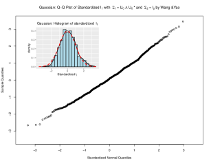
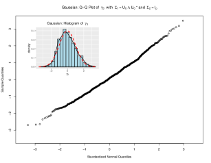
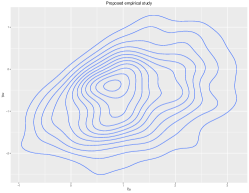
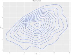
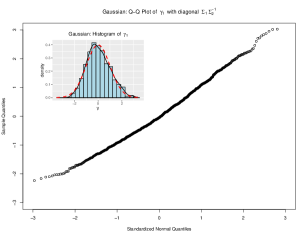
The simulated empirical distributions of the spiked eigenvalues from Normal assumption under Case I are drawn in Figure 1 in contrast to their corresponding limiting distributions.

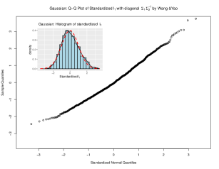
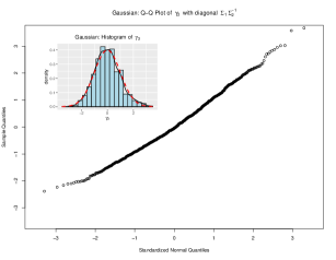
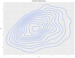
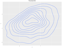
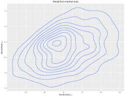
Figure 1: Case I under Gaussian assumption. Upper panels show that the Q-Q plots for the proposed $\gamma_{1}$ and $\gamma_{p}$, as well as the empirical densities of $\gamma_{1}$ and $\gamma_{p}$ (solid lines) comparing to their Gaussian limits (dashed lines). Lower panels show three contour plots: the first is the proposed empirical joint density function of $(\gamma_{21},\gamma_{22})$; the second is their corresponding limits; the third is the empirical joint density function of standardized $l_{p-2}$ and $l_{p-1}$.

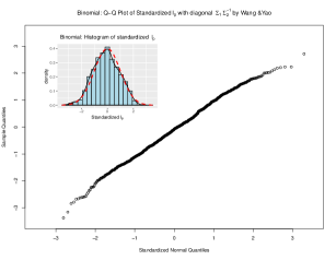
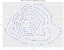
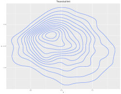
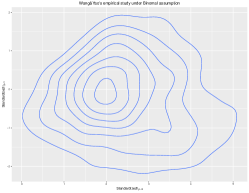
4.2 Case I under Binomial Assumption

Continue to use the assumptions in Case I, but $x_{ij}$ and $y_{ij}$ are from Binomial assumption. Then by the Theorem 3.2, similarly we have

• First, for the largest population spikes $\alpha_{1}=20$ and sample eigenvalue $l_{1,p}$,

  $$\gamma_{1}=\sqrt{p-4}\Big{(}\frac{l_{p,1}({\bf F})}{\psi_{n,1}}-1\Big{)}\rightarrow N(0,\sigma_{1}^{2})$$

  where

  $$\psi_{n,1}=42.667;\quad\sigma_{1}^{2}=1.116.$$

  For the least population spikes $\alpha_{p}=0.1$ and sample eigenvalues $l_{p,p}$, we have

  $$\gamma_{3}=\sqrt{p-4}\Big{(}\frac{l_{p,p}({\bf F})}{\psi_{n,3}}-1\Big{)}\rightarrow N(0,\sigma_{3}^{2})$$

  where

  $$\psi_{n,3}=0.0737;\quad\sigma_{3}^{2}=0.180.$$

• Second, for the population spikes $\alpha_{2}=0.2$ with multiplicity 2, and the sample eigenvalue $l_{1,p-1}$ and $l_{1,p-2}$, it is obtained that the two-dimensional random vector

  $$\gamma_{2}=\left(\gamma_{2,1},\gamma_{2,2}\right)^{\prime}=\left(\sqrt{p-4}\Big{(}\frac{l_{p,p-2}({\bf F})}{\psi_{n,2}}-1\Big{)},\sqrt{p-4}\Big{(}\frac{l_{p,p-1}({\bf F})}{\psi_{n,2}}-1\Big{)}\right)^{\prime}$$

  converges to the eigenvalues of random matrix $-\frac{1}{\kappa_{s}}\left[\Omega_{\psi_{2}}\right]_{22}$, where $\psi_{n,2}=0.13$, $\kappa_{s}=1.433$ for the spike $\alpha_{2}=0.2$. Furthermore, the matrix $\left[\Omega_{\psi_{2}}\right]_{22}$ is a $2\times 2$ symmetric matrix with the independent Gaussian entries, of which the $(s,t)$ element has mean zero and the variance given by

  $$var(w_{st})=\left\{\begin{array}[]{cc}0.264,&~{}\text{if}~{}s=t\\ 1.160,&~{}\text{if}~{}s\neq t\end{array}\right.$$

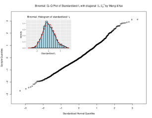
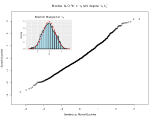
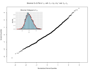
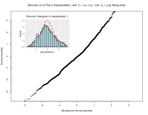
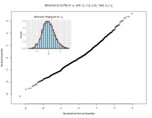
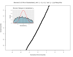
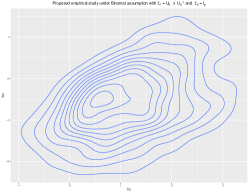
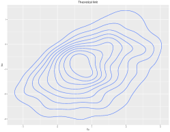
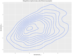
Figure 2 depicts the simulated empirical distributions of the spiked eigenvalues from binomial population under Case I comparing with their limiting distributions and the results from Wang and Yao (2017).

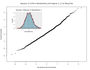
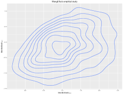
Figure 2: Case I under Binomial assumption. Upper panels show that the Q-Q plots for the proposed $\gamma_{1}$ and $\gamma_{p}$, as well as the empirical densities of $\gamma_{1}$ and $\gamma_{p}$ (solid lines) comparing to their Gaussian limits (dashed lines). Middle panels are the corresponding comparison of the empirical density of standardized $l_{1}$ and $l_{p}$ in Wang and Yao (2017). Lower panels show three contour plots: the first is the proposed empirical joint density function of $(\gamma_{21},\gamma_{22})$; the second is their corresponding limits; the third is the empirical joint density function of standardized $l_{p-2}$ and $l_{p-1}$.

4.3 Case II under all Assumptions

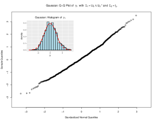
For the Case II, the simulations show that our proposed results are the same to the one of Normal assumption under Case I for all the population distribution assumptions by Theorem 3.1. The simulated results of three assumptions under Case II are respectively depicted in Figures 3-4.

Figure 3: Case II under Gaussian assumption. Upper panels show that the Q-Q plots for the proposed $\gamma_{1}$ and $\gamma_{3}$, as well as the empirical densities of $\gamma_{1}$ and $\gamma_{p}$ (solid lines) comparing to their Gaussian limits (dashed lines). Middle panels are the corresponding comparison of the empirical density of standardized $l_{1}$ and $l_{p}$ in Wang and Yao (2017). Lower panels show three contour plots: the first is the proposed empirical joint density function of $(\gamma_{21},\gamma_{22})$; the second is their corresponding limits; the third is the empirical joint density function of standardized $l_{p-2}$ and $l_{p-1}$.

Figure 4: Case II under Binomal assumption. Upper panels show that the Q-Q plots for the proposed $\gamma_{1}$ and $\gamma_{3}$, as well as the empirical densities of $\gamma_{1}$ and $\gamma_{p}$ (solid lines) comparing to their Gaussian limits (dashed lines). Middle panels are the corresponding comparison of the empirical density of standardized $l_{1}$ and $l_{p}$ in Wang and Yao (2017). Lower panels show three contour plots: the first is the proposed empirical joint density function of $(\gamma_{21},\gamma_{22})$; the second is their corresponding limits; the third is the empirical joint density function of standardized $l_{p-2}$ and $l_{p-1}$.

As seen from the Figures 3-4, our proposed method performs well for both of the population assumptions under Case II, but the method of Wang and Yao (2017) provides inaccurate variances for all the non-Gaussian assumptions under Case II because the assumption of diagonal block independence is not met.

5 Conclusion

In this paper, a G4MT for a generalized spiked Fisher matrix is proposed. By the relaxing the matching up to 4th moments condition to a tail probability in Assumption ${\bf B}$, which is necessary for the existence of the largest eigenvalue limit, we show that the universality of the asymptotic law for the spiked eigenvalues of high-dimensional generalized Fisher matrices. To illustrate the basic idea and procedures of the G4MT, we apply it to the CLT of normalized spiked eigenvalues related to high-dimensional generalized Fisher matrices as an example. Comparing to the previous work on universality, we simplify the calculations of high-order partial derivatives of an implicit function to the entries of the random matrix, avoid he strong condition $C_{0}$ of sub-exponential property, and further relax the requirements for the bounded 4th moments and diagonal block independent assumption. Instead, we only need a more regular and minor conditions (2.5) and (2.6) on the elements of $U_{1}$ and $V_{1}$, respectively. On the one hand, our result has much wider applications than Wang and Yao (2017); on the other hand, the result of Wang and Yao (2017) shows the necessity of the conditions (2.5) and (2.6).

References

• Anderson (2003) T. W. Anderson. (2003). An introduction to multivariate statistical analysis. Third Edition. Wiley New York.
• Bai and Ng (2002) Bai, J. and Ng, S. (2002). Determining the number of factors in approximate factor models. Econometrica, 70, 191-221.
• Bai, et al. (1991) Bai, Z.D., Miao, B.Q. and Rao, C. Radbakrisbna. (1991). Estimation of directions of arrival of signals: Asymptotic results. Advances in Spectrum Analysis and Array Processing, Vol. I, edited by Simon Haykin, Prentice Hall’s West Nyack, New York, pp 327-347.
• Bai and Silverstein (1998) Bai, Z. D. and Silverstein, J.W. (1998). No eigenvalues outside the support of the limiting spectral distribution of large-dimensional sample covariance matrices. Ann. Probab., Vol. 26, 1, 316-345.
• Bai and Silverstein (1999) Bai, Z. D. and Silverstein, J. W. (1999). Exact separation of eigenvalues of large dimensional sample covariance matrices. Ann. Probab. 27(3), 1536-1555.
• Bai and Silverstein (2004) Bai, Z. D. and Silverstein, J.W. (2004). CLT for linear spectral statistics of large-dimensional sample covariance matrices. The Annals of Probability, Vol. 32, No. 1A, 553-605.
• Bai and Silverstein (2010) Bai, Z. D. and Silverstein, J.W. (2010). Spectral Analysis of Large Dimensional Random Matrices. Springer Series in Statistics, Springer-Verlag, New York, ISSN: 0172-7397.
• Bai and Yao (2008) Bai, Z. D. and Yao, J. F. (2008). Central limit theorems for eigenvalues in a spiked population model. Annales de l’Institut Henri Poincare´´𝑒\acute{e} - Probabilite´´𝑒\acute{e}s et Statistiques, Vol. 44, No. 3, 447-474.
• Bai and Yao (2012) Bai, Z. D. and Yao, J. F. (2012). On sample eigenvalues in a generalized spiked population model. Journal of Multivariate Analysis, 106, 167-177.
• Bai and Zhou (2008) Bai, Z. D. and Zhou, W. (2008). Large sample covariance matrices without independence structures in columns. Statist. Sinica, 18, 425-442. MR2411613.
• Baik, et al. (2005) Baik, J., Arous, G. B., Pe´´e\acute{\rm e}che´´e\acute{\rm e}, S. (2005). Phase transition of the largest eigenvalue for nonnull complex sample covariance matrices. The Annals of Probability, 33, 1643-1697.
• Baik and Silverstein (2006) Baik, J and Silverstein, J. W. (2006). Eigenvalues of large sample covariance matrices of spiked population models. Journal of Multivariate Analysis, 97, 1382-1408.
• Ben and Péché (2005) Ben Arous, G. and Pe´´e\acute{\rm e}che´´e\acute{\rm e}, S. (2005). Universality of local eigenvalue statistics for some sample covariance matrices. Comm. Pure Appl. Math., 58, 1316-1357.
• Berthet and Rigollet (2013) Berthet, Q. and Rigollet, P. (2013). Optimal detection of sparse principal components in high dimension. The Annals of Statistics, 41, 1780-1815.
• Birnbaum, et al. (2013) Birnbaum, A., Johnstone, I. M., Nadler, B. and Paul, D. (2013). Minimax bounds for sparse PCA with noisy high-dimensional data. The Annals of Statistics, Vol. 41, No. 3, 1055-1084. DOI: 10.1214/12-AOS1014
• Cai, et al. (2017) Cai,T.T., Han,X. and Pan,G.M. (2017). Limiting Laws for Divergent Spiked Eigenvalues and Largest Non-spiked Eigenvalue of Sample Covariance Matrices. URL http://arxiv.org/abs/1711.00217v2
• Dyson (1970) Dyson, F. J. (1970). Correlations between eigenvalues of a random matrix. Comm. Math. Phys., 19, 235-250.
• Erdős, et al. (2010a) Erdős, L., Pe´´𝑒\acute{e}che´´𝑒\acute{e}, S., Rami´´𝑖\acute{i}rez, J. A., Schlein, B. and Yau, H.-T. (2010). Bulk universality for Wigner matrices. Comm. Pure Appl. Math., 63, 895-925.
• Erdős, et al. (2010b) Erdős, L., Rami´´𝑖\acute{i}rez, J. A., Schlein, B. and Yau, H.-T. (2010). Universality of sine-kernel for Wigner matrices with a small Gaussian perturbation. Electron. J. Probab., 15, 526-603.
• Fan, et al. (2013) Fan, J., Liao, Y. and Mincheva, M. (2013). Large covariance estimation by thresholding principal orthogonal complements. Journal of the Royal Statistical Society: Series B, 75, 1-44.
• Fan and Wang (2015) Fan, J. and Wang, W. (2015). Asymptotics of Empirical Eigen-structure for Ultra-high Dimensional Spiked Covariance Model. URL https://arxiv.org/abs/1502.04733v2
• Hoyle and Rattray (2004) Hoyle, D.C. and Rattray, M. (2004). Principal-component-analysis eigenvalue spectra from data with symmetry-breaking structure. Physics Review E, 69, 026124.
• Hu and Bai (2014) Hu, J. and Bai, Z.D. (2014). Estimation of directions of arrival of signals: Asymptotic results. Science China Mathematics, 57(11), DOI: 10.1007/s11425-014-4855-6.
• Hou, et al. (2019) Hou,Z.Q., Hu, J., Jiang,D.D., and Xiao, H. (2019). High-dimensional canonical correlation analysis based on a generalized Fisher matrix. In Processing.
• Jiang and Bai (2018) Jiang, D. and Bai, Z.D. (2018). Generalized Four Moment Theorem and an Application to CLT for Spiked Eigenvalues of Large-dimensional Covariance Matrices. In review, .
• Johnstone (2001) Johnstone, I. (2001). On the distribution of the largest eigenvalue in principal components analysis. Ann. Statist., 29, 295-327. MR1863961
• Johansson (2001) Johansson, K. (2001). Universality of the local spacing distribution in certain ensembles of Her- mitian Wigner matrices. Comm. Math. Phys., 215, 683-705.
• Jung and Marron (2009) Jung, S. and Marron, J. S. (2009). PCA consistency in High dimension, low sample size context. The Annals of Statistics, 37, 4104-4130.
• Li, et al. (2016) Li, H.Q., Bai, Z.D. and Hu, J. (2016). Convergence of empirical spectral distributions of large dimensional quaternion sample covariance matrices. Ann Inst Stat Math, 68, 765-785.
• Lindeberg (1922) Lindeberg, J.W. (1922). Eine neue Herleitung des Exponential gesetzes in der Wahrscheinlichkeitsrechnung Math. Z., 15, 211-225.
• Mehta (1967) Mehta, M. L. (1967). Random Matrices and the Statistical Theory of Energy Levels. Academic Press, New York.
• Nadler (2008) Nadler, B. (2008). Finite sample approximation results for principal component analysis: A matrix perturbation approach. The Annals of Statistics, 36, 2791?2817.
• Onatski (2009) Onatski, A. (2009). Testing hypotheses about the number of factors in large factor models. Econometrica, 77, 1447-1479.
• Onatski (2012) Onatski, A. (2012). Asymptotics of the principal components estimator of large factor models with weakly influential factors. Journal of Econometrics, 168, 244?258.
• Paul (2007) Paul, D. (2007). Asymptotics of sample eigenstructure for a large dimensional spiked covariance model. Statistica Sinica, 17, 1617-1642.
• Soshnikov (1999) Soshnikov, A. (1999). Universality at the edge of the spectrum in Wigner random matrices. Comm. Math. Phys., 207, 697-733.
• Skorokhod (1956) Skorokhod, A. V. (1956). Limit theorems for stochastic processes. Theory Probab Appl., 1, 261-290.
• Shen, et al. (2013) Shen, D., Shen, H., Zhu, H. and Marron, J. S. (2013). Surprising asymptotic conical structure in critical sample eigen-directions. URL http://arxiv.org/abs/1303.6171
• Tao and Vu (2015) Tao, T. and Vu,V. (2015). Random matrices: Universality of local eigenvalue statistics. The Annals of Probability, Vol. 43, No. 2, 782-874.
• Wigner (1958) Wigner, E. P. (1958). On the distribution of the roots of certain symmetric matrices. Ann. of Math., 67, 325-327.
• Wang and Yao (2017) Wang, Q., and Yao, J. (2017). Extreme eigenvalues of large-dimensional spiked fisher matrices with application. Annals of Statistics, 45(1), 415-445.