Analytic solutions for locally optimal designs
for gamma models
having linear predictor without intercept

Osama Idais osama.idais@ovgu.de Rainer Schwabe rainer.schwabe@ovgu.de Institute for Mathematical Stochastics, Otto-von-Guericke-University Magdeburg,
PF 4120, D-39016 Magdeburg, Germany
Abstract

The gamma model is a generalized linear model for gamma-distributed outcomes. The model is widely applied in psychology, ecology or medicine. In this paper we focus on gamma models having a linear predictor without intercept. For a specific scenario sets of locally D- and A-optimal designs are to be developed. Recently, Gaffke et al. (2018) established a complete class and an essentially complete class of designs for gamma models to obtain locally D-optimal designs. However to extend this approach to gamma model without an intercept term is complicated. To solve that further techniques have to be developed in the current work. Further, by a suitable transformation between gamma models with and without intercept optimality results may be transferred from one model to the other. Additionally by means of The General Equivalence Theorem optimality can be characterized for multiple regression by a system of polynomial inequalities which can be solved analytically or by computer algebra. By this necessary and sufficient conditions on the parameter values can be obtained for the local D-optimality of particular designs. The robustness of the derived designs with respect to misspecifications of the initial parameter values is examined by means of their local D-efficiencies.

keywords:
generalized linear model, optimal design, models without intercept, complete class , interaction.
journal:

1 Introduction

The gamma model is employed for outcomes that are non-negative, continuous, skewed and heteroscedastic specifically, when the variances are proportional to the square of the means. The gamma model with its canonical link ( reciprocal ) is appropriate for many real life data. In ecology and forestry, Gea-Izquierdo and Cañellas (2009) mentioned that gamma models offers a great potential for many forestry applications and they used gamma models to analyze plant competition. In medical context, Grover et al. (2013) fitted a gamma model with duration of diabetes as the response variable and predictors as the rate of rise in serum creatinine (SrCr) and number of successes (number of times SrCr values exceed its normal range (1.4 mg/dl)). For a study about air pollution, Kurtoğlu and Özkale (2016) employed a gamma model to analyze nitrogen dioxide concentrations considering some weather factors ( see also Chatterjee (1988), Section 8.7). In psychological studies, recently, Ng and Cribbie (2017) used a gamma model for modeling the relationship between negative automatic thoughts (NAT) and socially prescribed perfectionism (SPP).

Although, the canonical link is frequently employed in the gamma model but there is always a doubt about the suitable link function for outcomes. Therefore, a class of link functions might be employed. The common alternative links mostly come from the Box-Cox family and the power link family (see Atkinson and Woods (2015)). In fact, the family of power link functions includes the canonical link therefore it is a favorite choice for employment in this paper.

In the theory of optimal designs, the information matrix of a generalized linear model depends on the model parameters through the intensity function. Locally optimal designs can be derived through maximizing a specific optimality criterion at certain values of the parameters. However, although the gamma model is used in many applications, but it has no considerable attention for optimal designs. Geometric approaches were employed to derive locally D-optimal designs for a gamma model with single factor ( see Ford et al. (1992)), with two factors without intercept (see Burridge and Sebastiani (1992)) and for multiple factors (see Burridge and Sebastiani (1994)). Some of those results were highlighted on by Atkinson and Woods (2015). Recently, in Gaffke et al. (2018) we provided analytic solutions for optimal designs for gamma models. A complete class and essentially complete class of designs were established under certain assumptions. Therefore, the complexity of deriving optimal designs is reduced and one can only look for the optimal design in those classes.

In the present paper gamma models without intercept are considered. Absence of the intercept term yields a difficulty in deriving D- and A-optimal designs. Our main goal is developing various approaches to obtain, mostly, locally D-optimal designs. This paper is organized as follows. In section 2, the proposed model, the information matrix and the locally optimal design are presented. In section 3, locally D- and A-optimal designs are derived. In section 4, a two-factor model with interaction is considered for which locally D-optimal designs are derived. The performance of some derived D-optimal designs are examined in Section 5. Finally, a brief discussion and conclusions are given in Section 6.

2 Model, information and designs

Let y1,,ynsubscript𝑦1subscript𝑦𝑛y_{1},...,y_{n} be independent gamma-distributed response variables for n𝑛n experimental units, where the density is given by

P(yi;κ,λi)=λiκΓ(κ)yiκ1eλiyi,κ,λi,yi>0,(1in),formulae-sequence𝑃subscript𝑦𝑖𝜅subscript𝜆𝑖superscriptsubscript𝜆𝑖𝜅Γ𝜅superscriptsubscript𝑦𝑖𝜅1superscript𝑒subscript𝜆𝑖subscript𝑦𝑖𝜅subscript𝜆𝑖subscript𝑦𝑖01𝑖𝑛P(y_{i};\kappa,\lambda_{i})=\frac{\lambda_{i}^{\kappa}}{\Gamma\left(\kappa\right)}y_{i}^{\kappa-1}e^{-\lambda_{i}y_{i}}\,\,\,,\kappa,\,\lambda_{i},\,y_{i}>0,\,\,(1\leq i\leq n), (2.1)

The shape parameter κ𝜅\kappa of the gamma distribution is the same for all yisubscript𝑦𝑖y_{i} but the expectations μi=E(yi)subscript𝜇𝑖𝐸subscript𝑦𝑖\mu_{i}=E(y_{i}) depend on the values 𝒙isubscript𝒙𝑖\boldsymbol{x}_{i} of a covariate 𝒙𝒙\boldsymbol{x}. The canonical link obtained from a gamma distribution (2.1) is reciprocal (inverse)

ηi=κ/μi,where ηi=𝒇𝖳(𝒙i)𝜷,(1in),formulae-sequencesubscript𝜂𝑖𝜅subscript𝜇𝑖where subscript𝜂𝑖superscript𝒇𝖳subscript𝒙𝑖𝜷1𝑖𝑛\eta_{i}=\kappa/\mu_{i},\ \ \mbox{where }\ \ \eta_{i}=\boldsymbol{f}^{\sf T}(\boldsymbol{x}_{i})\boldsymbol{\beta},\,\,\ (1\leq i\leq n),

where 𝒇=(f1,,fp)𝖳𝒇superscriptsubscript𝑓1subscript𝑓𝑝𝖳\boldsymbol{f}=(f_{1},\ldots,f_{p})^{\sf T} is a given psuperscript𝑝\mathbb{R}^{p}-valued function on the experimental region 𝒳ν,ν1formulae-sequence𝒳superscript𝜈𝜈1{\cal X}\subset\mathbb{R}^{\nu},\,\nu\geq 1 with linearly independent component functions f1,,fpsubscript𝑓1subscript𝑓𝑝f_{1},\ldots,f_{p}, and 𝜷p𝜷superscript𝑝\boldsymbol{\beta}\in\mathbb{R}^{p} is a parameter vector (see McCullagh and Nelder (1989), Section 2.2.4). Here, the mean-variance function is v(μ)=μ2𝑣𝜇superscript𝜇2v(\mu)=\mu^{2} and the variance of a gamma distribution is thus given by var(y)=κ1μ2var𝑦superscript𝜅1superscript𝜇2\mathrm{var}(y)=\kappa^{-1}\mu^{2} with shape parameter κ>0𝜅0\kappa>0. Therefore, the intensity function at a point 𝒙𝒳𝒙𝒳\boldsymbol{x}\in\mathcal{X} (see Atkinson and Woods (2015)) is given by

u(𝒙,𝜷)=(var(y)(dηdμ)2)1=κ(𝒇𝖳(𝒙)𝜷)2.𝑢𝒙𝜷superscriptvar𝑦superscriptd𝜂d𝜇21𝜅superscriptsuperscript𝒇𝖳𝒙𝜷2u(\boldsymbol{x},\boldsymbol{\beta})=\Bigl{(}\mathrm{var}(y)\,\Big{(}\frac{{\rm d}\eta}{{\rm d}\mu}\Big{)}^{2}\Bigr{)}^{-1}=\kappa\bigl{(}\boldsymbol{f}^{\sf T}(\boldsymbol{x})\boldsymbol{\beta}\bigr{)}^{-2}. (2.2)

Practically, there are various link functions that are considered to fit gamma observations. The power link family which is considered throughout presents the class of link functions as in Burridge and Sebastiani (1994), see also Atkinson and Woods (2015), Section 2.5,

ηi=μiρ,where ηi=𝒇𝖳(𝒙i)𝜷,(1in).formulae-sequencesubscript𝜂𝑖superscriptsubscript𝜇𝑖𝜌where subscript𝜂𝑖superscript𝒇𝖳subscript𝒙𝑖𝜷1𝑖𝑛\eta_{i}=\mu_{i}^{\rho},\ \ \mbox{where }\ \ \eta_{i}=\boldsymbol{f}^{\sf T}(\boldsymbol{x}_{i})\boldsymbol{\beta},\ (1\leq i\leq n). (2.3)

The exponent ρ𝜌\rho of the power link function is a given nonzero real number. The intensity function under that family reads as

u0(𝒙,𝜷)=κρ2(𝒇𝖳(𝒙)𝜷)2.subscript𝑢0𝒙𝜷𝜅superscript𝜌2superscriptsuperscript𝒇𝖳𝒙𝜷2u_{0}(\boldsymbol{x},\boldsymbol{\beta})=\kappa\rho^{-2}\bigl{(}\boldsymbol{f}^{\sf T}(\boldsymbol{x})\boldsymbol{\beta}\bigr{)}^{-2}. (2.4)

Gamma-distributed responses are continuous and non-negative and therefore for a given experimental region 𝒳𝒳{\cal X} we assume throughout that the parameter vector 𝜷𝜷\boldsymbol{\beta} satisfies

𝒇𝖳(𝒙)𝜷>0 for all 𝒙𝒳.superscript𝒇𝖳𝒙𝜷0 for all 𝒙𝒳\boldsymbol{f}^{\sf T}(\boldsymbol{x})\,\boldsymbol{\beta}>0\ \mbox{ for all }\ \boldsymbol{x}\in\mathcal{X}. (2.5)

The Fisher information matrix for a single observation at a point 𝒙𝒳𝒙𝒳\boldsymbol{x}\in{\cal X} under parameter vector 𝜷𝜷\boldsymbol{\beta} is given by  u0(𝒙,𝜷)𝒇(𝒙)𝒇𝖳(𝒙)subscript𝑢0𝒙𝜷𝒇𝒙superscript𝒇𝖳𝒙u_{0}(\boldsymbol{x},\boldsymbol{\beta})\,\boldsymbol{f}(\boldsymbol{x})\,\boldsymbol{f}^{\sf T}(\boldsymbol{x}). Note that the positive factor κρ2𝜅superscript𝜌2\kappa\rho^{-2} is the same for all 𝒙𝒙\boldsymbol{x} and 𝜷𝜷\boldsymbol{\beta} and will not affect any design consideration below. We will ignore that factor and consider a normalized version of the Fisher information matrix at 𝒙𝒙\boldsymbol{x} and 𝜷𝜷\boldsymbol{\beta},

𝑴(𝒙,𝜷)=(𝒇𝖳(𝒙)𝜷)2𝒇(𝒙)𝒇𝖳(𝒙).𝑴𝒙𝜷superscriptsuperscript𝒇𝖳𝒙𝜷2𝒇𝒙superscript𝒇𝖳𝒙\boldsymbol{M}(\boldsymbol{x},\boldsymbol{\beta})=\bigl{(}\boldsymbol{f}^{\sf T}(\boldsymbol{x})\boldsymbol{\beta}\bigr{)}^{-2}\,\boldsymbol{f}(\boldsymbol{x})\,\boldsymbol{f}^{\sf T}(\boldsymbol{x}). (2.6)

We shall make use of approximate designs with finite support on the experimental region 𝒳𝒳\mathcal{X}. The approximate design ξ𝜉\xi on 𝒳𝒳\mathcal{X} is represented as

ξ={𝒙1𝒙2𝒙mω1ω2ωm},𝜉subscript𝒙1subscript𝒙2subscript𝒙𝑚subscript𝜔1subscript𝜔2subscript𝜔𝑚\xi=\left\{\begin{array}[]{cccc}\boldsymbol{x}_{1}&\boldsymbol{x}_{2}&\dots&\boldsymbol{x}_{m}\\ \omega_{1}&\omega_{2}&\dots&\omega_{m}\end{array}\right\}, (2.7)

where m𝑚m\in\mathbb{N}, 𝒙1,𝒙2,,𝒙m𝒳subscript𝒙1subscript𝒙2subscript𝒙𝑚𝒳\boldsymbol{x}_{1},\boldsymbol{x}_{2},\dots,\boldsymbol{x}_{m}\in\mathcal{X} are pairwise distinct points and ω1,ω2,,ωm>0subscript𝜔1subscript𝜔2subscript𝜔𝑚0\omega_{1},\omega_{2},\dots,\omega_{m}>0 with i=1mωi=1superscriptsubscript𝑖1𝑚subscript𝜔𝑖1\sum_{i=1}^{m}\omega_{i}=1. The set supp(ξ)={𝒙1,𝒙2,,𝒙m}supp𝜉subscript𝒙1subscript𝒙2subscript𝒙𝑚{\rm supp}(\xi)=\{\boldsymbol{x}_{1},\boldsymbol{x}_{2},\dots,\boldsymbol{x}_{m}\} is called the support of ξ𝜉\xi and ω1,,ωmsubscript𝜔1subscript𝜔𝑚\omega_{1},\ldots,\omega_{m} are called the weights of ξ𝜉\xi ( see Silvey (1980), p.15). A design ξ𝜉\xi is minimally supported if the number of support points is equal to the number of model parameters (i.e., m=p𝑚𝑝m=p). A minmal-support design which is also called a saturated design will appear frequently in the current work. The information matrix of a design ξ𝜉\xi at a parameter point 𝜷𝜷\boldsymbol{\beta} is defined by

𝑴(ξ,𝜷)=i=1mωi𝑴(𝒙i,𝜷).𝑴𝜉𝜷superscriptsubscript𝑖1𝑚subscript𝜔𝑖𝑴subscript𝒙𝑖𝜷\displaystyle\boldsymbol{M}(\xi,\boldsymbol{\beta})=\sum_{i=1}^{m}\omega_{i}\boldsymbol{M}(\boldsymbol{x}_{i},\boldsymbol{\beta}). (2.8)

Another representation of the information matrix (2.8) can be considered by defining the m×p𝑚𝑝m\times p design matrix 𝑭=[𝒇(𝒙1),,𝒇(𝒙m)]𝖳𝑭superscript𝒇subscript𝒙1𝒇subscript𝒙𝑚𝖳\boldsymbol{F}=[\boldsymbol{f}(\boldsymbol{\boldsymbol{x}}_{1}),\dots,\boldsymbol{f}(\boldsymbol{\boldsymbol{x}}_{m})]^{\sf T} and the m×m𝑚𝑚m\times m weight matrix 𝑽=diag(ωiu(𝒙i,𝜷))i=1m𝑽diagsuperscriptsubscriptsubscript𝜔𝑖𝑢subscript𝒙𝑖𝜷𝑖1𝑚\boldsymbol{V}=\mathrm{diag}(\omega_{i}u(\boldsymbol{x}_{i},\boldsymbol{\beta}))_{i=1}^{m} and hence, 𝑴(ξ,𝜷)=𝑭𝖳𝑽𝑭𝑴𝜉𝜷superscript𝑭𝖳𝑽𝑭\boldsymbol{M}(\xi,\boldsymbol{\beta})=\boldsymbol{F}^{\sf T}\boldsymbol{V}\boldsymbol{F}.

A locally optimal design minimizes a convex criterion function of the information matrix at a given parameter point 𝜷𝜷\boldsymbol{\beta}. Denote by ”det\det” and ”trtr{\rm tr}” the determinant and the trace of a matrix, respectively. We will employ the popular D-criterion and the A-criterion. More precisely, a design ξsuperscript𝜉\xi^{*} is said to be locally D-optimal (at 𝜷𝜷\boldsymbol{\beta}) if its information matrix 𝑴(ξ,𝜷)𝑴superscript𝜉𝜷\boldsymbol{M}(\xi^{*},\boldsymbol{\beta}) at 𝜷𝜷\boldsymbol{\beta} is nonsingular and det(𝑴1(ξ,𝜷))=minξdet(𝑴1(ξ,𝜷))superscript𝑴1superscript𝜉𝜷subscript𝜉superscript𝑴1𝜉𝜷\det\bigl{(}\boldsymbol{M}^{-1}(\xi^{*},\boldsymbol{\beta})\bigr{)}=\min_{\xi}\det\bigl{(}\boldsymbol{M}^{-1}(\xi,\boldsymbol{\beta})\bigr{)} where the minimum on the r.h.s. is taken over all designs ξ𝜉\xi whose information matrix at 𝜷𝜷\boldsymbol{\beta} is nonsingular. Similarly, a design ξsuperscript𝜉\xi^{*} is said to be locally A-optimal (at 𝜷𝜷\boldsymbol{\beta}) if its information matrix at 𝜷𝜷\boldsymbol{\beta} is nonsingular and tr(𝑴1(ξ,𝜷))=minξtr(𝑴1(ξ,𝜷))trsuperscript𝑴1superscript𝜉𝜷subscript𝜉trsuperscript𝑴1𝜉𝜷{\rm tr}\bigl{(}\boldsymbol{M}^{-1}(\xi^{*},\boldsymbol{\beta})\bigr{)}=\min_{\xi}{\rm tr}\bigl{(}\boldsymbol{M}^{-1}(\xi,\boldsymbol{\beta})\bigr{)} where, again, the minimum is taken over all designs ξ𝜉\xi whose information matrix at 𝜷𝜷\boldsymbol{\beta} is nonsingular.

Remark 1.

It is worthwhile mentioning that the set of designs for which the information matrix is nonsingular does not depend on 𝜷𝜷\boldsymbol{\beta} (when u(𝒙,𝜷)𝑢𝒙𝜷u(\boldsymbol{x},\boldsymbol{\beta}) is strictly positive). In particular it is just the set of designs for which the information matrix is nonsingular in the corresponding ordinary regression model (ignoring the intensity u(𝒙,𝜷)𝑢𝒙𝜷u(\boldsymbol{x},\boldsymbol{\beta})). That is the singularity depends on the support points of a design ξ𝜉\xi because its information matrix 𝑴(ξ,𝜷)=𝑭𝖳𝑽𝑭𝑴𝜉𝜷superscript𝑭𝖳𝑽𝑭\boldsymbol{M}(\xi,\boldsymbol{\beta})=\boldsymbol{F}^{\sf T}\boldsymbol{V}\boldsymbol{F} is full rank if and only if 𝑭𝑭\boldsymbol{F} is full rank.

Remark 2.

If the experimental region is a compact set and the functions 𝒇(𝒙)𝒇𝒙\boldsymbol{f}(\boldsymbol{x}) and u(𝒙,𝜷)𝑢𝒙𝜷u(\boldsymbol{x},\boldsymbol{\beta}) are continuous in 𝒙𝒙\boldsymbol{x} then the set of all nonnegative definite information matrices is compact. Therefore, there exists a locally D- resp. A-optimal design for any given parameter point 𝜷𝜷\boldsymbol{\beta}.

In order to verify the local optimality of a design The General Equivalence Theorem is usually employed. It provides necessary and sufficient conditions for a design to be optimal with respect to the optimality criterion, in specific D- and A-criteria and thus the optimality of a suggested design can easily be verified or disproved (see Silvey (1980), p.40, p.48 and p.54)). The most generic one is the celebrated Kiefer-Wolfowitz equivalence theorem under D-criterion ( see Kiefer and Wolfowitz (1960) ). In the following we obtain equivalent characterizations of locally D- and A-optimal designs.

Theorem 2.1.

Let 𝛃𝛃\boldsymbol{\beta} be a given parameter point and let ξsuperscript𝜉\xi^{*} be a design with nonsingular information matrix 𝐌(ξ,𝛃)𝐌superscript𝜉𝛃\boldsymbol{M}(\xi^{*},\boldsymbol{\beta}).
(a) The design ξsuperscript𝜉\xi^{*} is locally D-optimal (at 𝛃𝛃\boldsymbol{\beta}) if and only if

u(𝒙,𝜷)𝒇𝖳(𝒙)𝑴1(ξ,𝜷)𝒇(𝒙)p for all 𝒙𝒳.formulae-sequence𝑢𝒙𝜷superscript𝒇𝖳𝒙superscript𝑴1superscript𝜉𝜷𝒇𝒙𝑝 for all 𝒙𝒳\displaystyle u(\boldsymbol{x},\boldsymbol{\beta})\,\boldsymbol{f}^{\sf T}(\boldsymbol{x})\boldsymbol{M}^{-1}(\xi^{*},\boldsymbol{\beta})\boldsymbol{f}(\boldsymbol{x})\leq p\ \ \mbox{ for all }\,\boldsymbol{x}\in\mathcal{X}.

(b) The design ξsuperscript𝜉\xi^{*} is locally A-optimal (at 𝛃𝛃\boldsymbol{\beta}) if and only if

u(𝒙,𝜷)𝒇𝖳(𝒙)𝑴2(ξ,𝜷)𝒇(𝒙)tr(𝑴1(ξ,𝜷)) for all 𝒙𝒳.formulae-sequence𝑢𝒙𝜷superscript𝒇𝖳𝒙superscript𝑴2superscript𝜉𝜷𝒇𝒙trsuperscript𝑴1superscript𝜉𝜷 for all 𝒙𝒳\displaystyle u(\boldsymbol{x},\boldsymbol{\beta})\,\boldsymbol{f}^{\sf T}(\boldsymbol{x})\boldsymbol{M}^{-2}(\xi^{*},\boldsymbol{\beta})\boldsymbol{f}(\boldsymbol{x})\leq\mathrm{tr}\bigl{(}\boldsymbol{M}^{-1}(\xi^{*},\boldsymbol{\beta})\bigr{)}\ \ \mbox{ for all }\,\boldsymbol{x}\in\mathcal{X}.
Remark 3.

The inequalities given by part (a) and part (b) of Theorem 2.1 are equations at support points of any D- or A-optimal design, respectively.

Throughout, we consider gamma models that do not explicitly involve a constant (intercept) term. More precisely, we assume that fj1subscript𝑓𝑗1f_{j}\neq 1 for all (1jp1𝑗𝑝1\leq j\leq p) and thus fj(𝟎)=𝟎subscript𝑓𝑗00f_{j}(\boldsymbol{0})=\boldsymbol{0} for all (1jp1𝑗𝑝1\leq j\leq p). In particular, we restrict to a first order model with

𝒇(𝒙)=𝒙, where 𝒙=(x1,,xν)𝖳,ν2,formulae-sequence𝒇𝒙𝒙formulae-sequence where 𝒙superscriptsubscript𝑥1subscript𝑥𝜈𝖳𝜈2\boldsymbol{f}(\boldsymbol{x})=\boldsymbol{x},\,\,\mbox{ where }\,\,\boldsymbol{x}=(x_{1},\dots,x_{\nu})^{\sf T},\,\,\nu\geq 2, (2.9)

and the two-factor model with interaction

𝒇(𝒙)=(x1,x2,x1x2)𝖳.𝒇𝒙superscriptsubscript𝑥1subscript𝑥2subscript𝑥1subscript𝑥2𝖳\boldsymbol{f}(\boldsymbol{x})=(x_{1},x_{2},x_{1}x_{2})^{\sf T}. (2.10)

Surely, condition (2.5), i.e., 𝒇𝖳(𝒙)𝜷>0superscript𝒇𝖳𝒙𝜷0\boldsymbol{f}^{\sf T}(\boldsymbol{x})\boldsymbol{\beta}>0 for all 𝒙𝒳𝒙𝒳\boldsymbol{x}\in\mathcal{X} implies that 𝟎𝒳0𝒳\boldsymbol{0}\notin\mathcal{X}. Therefore, an experimental region as 𝒳=[0,)ν{𝟎}𝒳superscript0𝜈0\mathcal{X}=[0,\infty)^{\nu}\setminus\{\boldsymbol{0}\} is considered. Note that this experimental region is no longer compact therefore the existence of optimal designs is not assured and has to be checked separately.

In contrast, we often consider a compact experimental region that is a ν𝜈\nu-dimensional hypercube

𝒳=[a,b]ν,ν2 with a,b and 0<a<b,formulae-sequence𝒳superscript𝑎𝑏𝜈formulae-sequence𝜈2 with 𝑎𝑏 and 0𝑎𝑏\mathcal{X}=\bigl{[}a,b\bigr{]}^{\nu},\,\nu\geq 2\mbox{ with }a,b\in\mathbb{R}\mbox{ and }0<a<b, (2.11)

with vertices 𝒗i,i=1,,K,K=2νformulae-sequencesubscript𝒗𝑖𝑖1𝐾𝐾superscript2𝜈\boldsymbol{v}_{i},\,i=1,\dots,K,\,K=2^{\nu} given by the points whose i𝑖i-th coordinates are either a𝑎a or b𝑏b for all i=1,,ν𝑖1𝜈i=1,\dots,\nu.

In Gaffke et al. (2018), we showed that under gamma models with regression function 𝒇(𝒙)𝒇𝒙\boldsymbol{f}(\boldsymbol{x}) from (2.9) or (2.10) and experimental region 𝒳=[a,b]ν,ν2, 0<a<bformulae-sequence𝒳superscript𝑎𝑏𝜈formulae-sequence𝜈2 0𝑎𝑏\mathcal{X}=[a,b]^{\nu},\nu\geq 2,\,0<a<b the design that has support only among the vertices is at least good as any design that has no support points from the vertices w.r.t the Loewner semi-ordering of information matrices or, more generally, of nonnegative definite p×p𝑝𝑝p\times p matrices. That is if 𝑨𝑨\boldsymbol{A} and 𝑩𝑩\boldsymbol{B} are nonnegative definite p×p𝑝𝑝p\times p matrices we write AB𝐴𝐵A\leq B if and only if BA𝐵𝐴B-A is nonnegative definite. The set of all designs ξ𝜉\xi such that supp(ξ){𝒗1,,𝒗K}supp𝜉subscript𝒗1subscript𝒗𝐾\mathrm{supp}(\xi)\subseteq\{\boldsymbol{v}_{1},\dots,\boldsymbol{v}_{K}\} is a locally essentially complete class of designs at a given 𝜷𝜷\boldsymbol{\beta}. As a result, there exists a design ξsuperscript𝜉\xi^{*} that is only supported by vertices of 𝒳𝒳\mathcal{X} which is locally optimal (at 𝜷𝜷\boldsymbol{\beta}) w.r.t. D- or A-criterion. On that basis, throughout, we restrict to designs whose support is a subset of the vertices of 𝒳𝒳\mathcal{X} given by a hypercube (2.11).

Remark 4.

Let us denote by ψ(𝒙)𝜓𝒙\psi(\boldsymbol{x}) the left hand side of The Equivalence Theorems, Theorem 2.1, part (a) or part (b). Typically ψ(𝒙)𝜓𝒙\psi(\boldsymbol{x}) is called the sensitivity function. Actually, under non-intercept gamma models ψ(𝒙)𝜓𝒙\psi(\boldsymbol{x}) is invariant with respect to simultaneous scale transformation of 𝒙𝒙\boldsymbol{x}, i.e., ψ(λ𝒙)=ψ(𝒙)𝜓𝜆𝒙𝜓𝒙\psi(\lambda\boldsymbol{x})=\psi(\boldsymbol{x}) for any λ>0𝜆0\lambda>0. This essentially comes from the fact that the function 𝒇𝜷(𝒙)=(𝒇𝖳(𝒙)𝜷)1𝒇(𝒙)subscript𝒇𝜷𝒙superscriptsuperscript𝒇𝖳𝒙𝜷1𝒇𝒙\boldsymbol{f}_{\boldsymbol{\beta}}(\boldsymbol{x})=\big{(}\boldsymbol{f}^{\sf T}(\boldsymbol{x})\boldsymbol{\beta}\big{)}^{-1}\boldsymbol{f}(\boldsymbol{x}) is invariant with respect to simultaneous rescaling of the components of 𝒙𝒙\boldsymbol{x}, i.e., 𝒇𝜷(λ𝒙)=𝒇𝜷(𝒙)subscript𝒇𝜷𝜆𝒙subscript𝒇𝜷𝒙\boldsymbol{f}_{\boldsymbol{\beta}}(\lambda\boldsymbol{x})=\boldsymbol{f}_{\boldsymbol{\beta}}(\boldsymbol{x}). This property is explicitly transferred to the information matrix (2.6) since it can be represented in form 𝑴(𝒙,𝜷)=𝒇𝜷(𝒙)𝒇𝜷𝖳(𝒙)𝑴𝒙𝜷subscript𝒇𝜷𝒙superscriptsubscript𝒇𝜷𝖳𝒙\boldsymbol{M}(\boldsymbol{x},\boldsymbol{\beta})=\boldsymbol{f}_{\boldsymbol{\beta}}(\boldsymbol{x})\boldsymbol{f}_{\boldsymbol{\beta}}^{\sf T}(\boldsymbol{x}), and hence 𝑴(λ𝒙,𝜷)=𝑴(𝒙,𝜷)𝑴𝜆𝒙𝜷𝑴𝒙𝜷\boldsymbol{M}(\lambda\boldsymbol{x},\boldsymbol{\beta})=\boldsymbol{M}(\boldsymbol{x},\boldsymbol{\beta}). In fact, this property plays a main rule in the solution of the forthcoming optimal designs.

3 First order gamma model

In this section we consider a gamma model with

𝒇(𝒙)=(x1,,xν)𝖳,ν2,𝒙𝒳,formulae-sequence𝒇𝒙superscriptsubscript𝑥1subscript𝑥𝜈𝖳formulae-sequence𝜈2𝒙𝒳\displaystyle\boldsymbol{f}(\boldsymbol{x})=(x_{1},\dots,x_{\nu})^{\sf T},\,\nu\geq 2,\,\,\boldsymbol{x}\in\mathcal{X}, (3.1)
where
𝒇𝜷(𝒙)=1β1x1++βνxν(x1xν).subscript𝒇𝜷𝒙1subscript𝛽1subscript𝑥1subscript𝛽𝜈subscript𝑥𝜈subscript𝑥1subscript𝑥𝜈\displaystyle\boldsymbol{f}_{\boldsymbol{\beta}}(\boldsymbol{x})=\frac{1}{\beta_{1}x_{1}+\dots+\beta_{\nu}x_{\nu}}\,\left({\begin{array}[]{c}x_{1}\\ \vdots\\ x_{\nu}\end{array}}\right). (3.5)

Firstly let the experimental region 𝒳=[0,)ν{𝟎}𝒳superscript0𝜈0\mathcal{X}=[0,\infty)^{\nu}\setminus\{\boldsymbol{0}\} be considered. Denote by 𝒆isubscript𝒆𝑖\boldsymbol{e}_{i} for all (1iν)1𝑖𝜈(1\leq i\leq\nu) the ν𝜈\nu-dimensional unit vectors. The parameter space is determined by condition (2.5), i.e., 𝒙𝖳𝜷>0superscript𝒙𝖳𝜷0\boldsymbol{x}^{\sf T}\boldsymbol{\beta}>0 for all 𝒙𝒳𝒙𝒳\boldsymbol{x}\in\mathcal{X} which implies that 𝜷(0,)ν𝜷superscript0𝜈\boldsymbol{\beta}\in(0,\infty)^{\nu}, i.e., βi>0subscript𝛽𝑖0\beta_{i}>0 for all (1iν1𝑖𝜈1\leq i\leq\nu). Let the induced experimental region is given by 𝒇𝜷(𝒳)={𝒇𝜷(𝒙):𝒙𝒳}subscript𝒇𝜷𝒳conditional-setsubscript𝒇𝜷𝒙𝒙𝒳\boldsymbol{f}_{\boldsymbol{\beta}}(\mathcal{X})=\{\boldsymbol{f}_{\boldsymbol{\beta}}(\boldsymbol{x}):\boldsymbol{x}\in\mathcal{X}\}. Although 𝒳𝒳\mathcal{X} is not compact but 𝒇𝜷(𝒳)subscript𝒇𝜷𝒳\boldsymbol{f}_{\boldsymbol{\beta}}(\mathcal{X}) is compact. That is

𝒇𝜷(𝒳)=Conv{𝒇𝜷(𝒆i):𝒆i𝒳,i=1,,ν},subscript𝒇𝜷𝒳Convconditional-setsubscript𝒇𝜷subscript𝒆𝑖formulae-sequencesubscript𝒆𝑖𝒳𝑖1𝜈\boldsymbol{f}_{\boldsymbol{\beta}}(\mathcal{X})=\mathrm{Conv}\{\boldsymbol{f}_{\boldsymbol{\beta}}(\boldsymbol{e}_{i}):\boldsymbol{e}_{i}\in\mathcal{X},i=1,\dots,\nu\},

where ‘Conv’ denotes convex hull operation. That means each point 𝒇𝜷(𝒙)subscript𝒇𝜷𝒙\boldsymbol{f}_{\boldsymbol{\beta}}(\boldsymbol{x}) for all 𝒙𝒳𝒙𝒳\boldsymbol{x}\in\mathcal{X} can be written as a convex combination of 𝒇𝜷(𝒆i)subscript𝒇𝜷subscript𝒆𝑖\boldsymbol{f}_{\boldsymbol{\beta}}(\boldsymbol{e}_{i}) for all (1iν1𝑖𝜈1\leq i\leq\nu), i.e., we obtain 𝒇𝜷(𝒙)=i=1ναi𝒇𝜷(𝒆i)subscript𝒇𝜷𝒙superscriptsubscript𝑖1𝜈subscript𝛼𝑖subscript𝒇𝜷subscript𝒆𝑖\boldsymbol{f}_{\boldsymbol{\beta}}(\boldsymbol{x})=\sum_{i=1}^{\nu}\alpha_{i}\boldsymbol{f}_{\boldsymbol{\beta}}(\boldsymbol{e}_{i}) for some αi0subscript𝛼𝑖0\alpha_{i}\geq 0 for all (1iν1𝑖𝜈1\leq i\leq\nu) such that i=1ναi=1superscriptsubscript𝑖1𝜈subscript𝛼𝑖1\sum_{i=1}^{\nu}\alpha_{i}=1 (here, αi=βixi/i=1νβixi,i=1,,νformulae-sequencesubscript𝛼𝑖subscript𝛽𝑖subscript𝑥𝑖superscriptsubscript𝑖1𝜈subscript𝛽𝑖subscript𝑥𝑖𝑖1𝜈\alpha_{i}=\beta_{i}x_{i}/\sum_{i=1}^{\nu}\beta_{i}x_{i},i=1,\dots,\nu). As a consequence, the set of all nonnegative definite information matrices is compact and a locally optimal design can be obtained (cp. Remark 2).

Theorem 3.1.

Consider the experimental region 𝒳=[0,)ν{𝟎}𝒳superscript0𝜈0\mathcal{X}=[0,\infty)^{\nu}\setminus\{\boldsymbol{0}\}. Let 𝐱i=𝐞isuperscriptsubscript𝐱𝑖subscript𝐞𝑖\boldsymbol{x}_{i}^{*}=\boldsymbol{e}_{i}  for all (1iν)1𝑖𝜈(1\leq i\leq\nu). Given a parameter point 𝛃𝛃\boldsymbol{\beta}. Then

  1. (i)

    The saturated design ξsuperscript𝜉\xi^{*} that assigns equal weight ν1superscript𝜈1\nu^{-1} to the support 𝒙isuperscriptsubscript𝒙𝑖\boldsymbol{x}_{i}^{*} for all  (1iν)1𝑖𝜈(1\leq i\leq\nu) is locally D-optimal (at 𝜷𝜷\boldsymbol{\beta}).

  2. (ii)

    The saturated design ζsuperscript𝜁\zeta^{*} that assigns the weights ωi=βi/i=1νβisuperscriptsubscript𝜔𝑖subscript𝛽𝑖superscriptsubscript𝑖1𝜈subscript𝛽𝑖\omega_{i}^{*}=\beta_{i}/\sum_{i=1}^{\nu}\beta_{i}  for all (1iν)1𝑖𝜈(1\leq i\leq\nu) to the corresponding design point 𝒙isuperscriptsubscript𝒙𝑖\boldsymbol{x}_{i}^{*}  for all (1iν)1𝑖𝜈(1\leq i\leq\nu) is locally A-optimal (at 𝜷𝜷\boldsymbol{\beta}).

Proof.

Define the ν×ν𝜈𝜈\nu\times\nu design matrix 𝑭=diag(𝒆i)i=1ν𝑭diagsuperscriptsubscriptsubscript𝒆𝑖𝑖1𝜈\boldsymbol{F}=\mathrm{diag}(\boldsymbol{e}_{i})_{i=1}^{\nu} with ν×ν𝜈𝜈\nu\times\nu weight matrix 𝑽=diag(ωi/βi2)i=1ν𝑽diagsuperscriptsubscriptsuperscriptsubscript𝜔𝑖superscriptsubscript𝛽𝑖2𝑖1𝜈\boldsymbol{V}=\mathrm{diag}(\omega_{i}^{*}/\beta_{i}^{2})_{i=1}^{\nu}. Then we have 𝑭𝖳𝑽𝑭=diag(ωi/βi2)i=1νsuperscript𝑭𝖳𝑽𝑭diagsuperscriptsubscriptsuperscriptsubscript𝜔𝑖superscriptsubscript𝛽𝑖2𝑖1𝜈\boldsymbol{F}^{\sf T}\boldsymbol{V}\boldsymbol{F}=\mathrm{diag}(\omega_{i}^{*}/\beta_{i}^{2})_{i=1}^{\nu} and (𝑭𝖳𝑽𝑭)1=diag(βi2/ωi)i=1νsuperscriptsuperscript𝑭𝖳𝑽𝑭1diagsuperscriptsubscriptsuperscriptsubscript𝛽𝑖2superscriptsubscript𝜔𝑖𝑖1𝜈\big{(}\boldsymbol{F}^{\sf T}\boldsymbol{V}\boldsymbol{F}\big{)}^{-1}=\mathrm{diag}(\beta_{i}^{2}/\omega_{i}^{*})_{i=1}^{\nu} where;

For D-optimality, ωi=ν1i,𝑴1(ξ,𝜷)=νdiag(βi2)i=1ν and 𝒇𝖳(𝒙)diag(βi2)i=1ν𝒇(𝒙)=i=1νβi2xi2.formulae-sequenceFor D-optimality, superscriptsubscript𝜔𝑖superscript𝜈1for-all𝑖superscript𝑴1superscript𝜉𝜷𝜈diagsuperscriptsubscriptsuperscriptsubscript𝛽𝑖2𝑖1𝜈 and superscript𝒇𝖳𝒙diagsuperscriptsubscriptsuperscriptsubscript𝛽𝑖2𝑖1𝜈𝒇𝒙superscriptsubscript𝑖1𝜈superscriptsubscript𝛽𝑖2superscriptsubscript𝑥𝑖2\displaystyle\mbox{For D-optimality, }\,\,\omega_{i}^{*}=\nu^{-1}\forall i,\,\boldsymbol{M}^{-1}\bigl{(}\xi^{*},\boldsymbol{\beta}\bigr{)}=\nu\,\mathrm{diag}(\beta_{i}^{2})_{i=1}^{\nu}\mbox{ and }\,\boldsymbol{f}^{\sf T}(\boldsymbol{x})\mathrm{diag}(\beta_{i}^{2})_{i=1}^{\nu}\boldsymbol{f}(\boldsymbol{x})=\sum_{i=1}^{\nu}\beta_{i}^{2}x_{i}^{2}.
For A-optimality, ωi=βi/i=1νβii,𝑴1(ζ,𝜷)=(i=1νβi)diag(βi)i=1ν,tr(𝑴1(ζ,𝜷))=(i=1νβi)2,formulae-sequenceFor A-optimality, superscriptsubscript𝜔𝑖subscript𝛽𝑖superscriptsubscript𝑖1𝜈subscript𝛽𝑖for-all𝑖formulae-sequencesuperscript𝑴1superscript𝜁𝜷superscriptsubscript𝑖1𝜈subscript𝛽𝑖diagsuperscriptsubscriptsubscript𝛽𝑖𝑖1𝜈trsuperscript𝑴1superscript𝜁𝜷superscriptsuperscriptsubscript𝑖1𝜈subscript𝛽𝑖2\displaystyle\mbox{For A-optimality, }\,\,\omega_{i}^{*}=\beta_{i}/\sum_{i=1}^{\nu}\beta_{i}\,\forall i,\,\,\boldsymbol{M}^{-1}\bigl{(}\zeta^{*},\boldsymbol{\beta}\bigr{)}=\big{(}\sum\limits_{i=1}^{\nu}\beta_{i}\big{)}\mathrm{diag}(\beta_{i})_{i=1}^{\nu},\,\,\mathrm{tr}\big{(}\boldsymbol{M}^{-1}(\zeta^{*},\boldsymbol{\beta})\big{)}=\big{(}\sum_{i=1}^{\nu}\beta_{i}\big{)}^{2},
𝑴2(ζ,𝜷)=(i=1νβi)2diag(βi2)i=1ν, and 𝒇𝖳(𝒙)(i=1νβi)2diag(βi2)i=1ν𝒇(𝒙)=(i=1νβi)2i=1νβi2xi2.formulae-sequencesuperscript𝑴2superscript𝜁𝜷superscriptsuperscriptsubscript𝑖1𝜈subscript𝛽𝑖2diagsuperscriptsubscriptsuperscriptsubscript𝛽𝑖2𝑖1𝜈 and superscript𝒇𝖳𝒙superscriptsuperscriptsubscript𝑖1𝜈subscript𝛽𝑖2diagsuperscriptsubscriptsuperscriptsubscript𝛽𝑖2𝑖1𝜈𝒇𝒙superscriptsuperscriptsubscript𝑖1𝜈subscript𝛽𝑖2superscriptsubscript𝑖1𝜈superscriptsubscript𝛽𝑖2superscriptsubscript𝑥𝑖2\displaystyle\boldsymbol{M}^{-2}\bigl{(}\zeta^{*},\boldsymbol{\beta}\bigr{)}=\big{(}\sum_{i=1}^{\nu}\beta_{i}\big{)}^{2}\mathrm{diag}(\beta_{i}^{2})_{i=1}^{\nu},\,\mbox{ and }\boldsymbol{f}^{\sf T}(\boldsymbol{x})\big{(}\sum_{i=1}^{\nu}\beta_{i}\big{)}^{2}\mathrm{diag}(\beta_{i}^{2})_{i=1}^{\nu}\boldsymbol{f}(\boldsymbol{x})=\big{(}\sum_{i=1}^{\nu}\beta_{i}\big{)}^{2}\sum_{i=1}^{\nu}\beta_{i}^{2}x_{i}^{2}.

Hence, by The Equivalence Theorem (Theorem 2.1, part (a) and part (b)) ξsuperscript𝜉\xi^{*} resp. ζsuperscript𝜁\zeta^{*} is locally D- resp. A-optimal (at 𝜷𝜷\boldsymbol{\beta}) if and only if (i=1νβixi)2(i=1νβi2xi2)1superscriptsuperscriptsubscript𝑖1𝜈subscript𝛽𝑖subscript𝑥𝑖2superscriptsubscript𝑖1𝜈superscriptsubscript𝛽𝑖2superscriptsubscript𝑥𝑖21\,\,\big{(}\sum_{i=1}^{\nu}\beta_{i}x_{i}\big{)}^{-2}\big{(}\sum_{i=1}^{\nu}\beta_{i}^{2}x_{i}^{2}\big{)}\leq 1 for all  𝒙𝒳𝒙𝒳\boldsymbol{x}\in\mathcal{X} which is equivalent to 2i<j=1νβiβjxixj02superscriptsubscript𝑖𝑗1𝜈subscript𝛽𝑖subscript𝛽𝑗subscript𝑥𝑖subscript𝑥𝑗0-2\sum_{i<j=1}^{\nu}\beta_{i}\beta_{j}x_{i}x_{j}\leq 0  for all  𝒙𝒳𝒙𝒳\boldsymbol{x}\in\mathcal{X}. The latter inequality holds true by model assumptions βi>0,xi0formulae-sequencesubscript𝛽𝑖0subscript𝑥𝑖0\beta_{i}>0,x_{i}\geq 0 for all (1iν1𝑖𝜈1\leq i\leq\nu). ∎

Remark 5.

The locally D-optimal designs provided by part (i) of Theorem 3.1 is robust against misspecified values of the model parameter in its parameter space (0,)νsuperscript0𝜈(0,\infty)^{\nu}.

While the information matrix is invariant w.r.t. to simultaneous rescaling of the components of 𝒙𝒙\boldsymbol{x} as it is mentioned in Remark 4, the result of Theorem 3.1 can be extended:

Corollary 3.1.

Consider the experimental region 𝒳=[0,)ν{𝟎}𝒳superscript0𝜈0\mathcal{X}=[0,\infty)^{\nu}\setminus\{\boldsymbol{0}\}. Given a constant vector 𝐚=(a1,,aν)𝖳𝐚superscriptsubscript𝑎1subscript𝑎𝜈𝖳\boldsymbol{a}=(a_{1},\dots,a_{\nu})^{\sf T}  such that ai>0subscript𝑎𝑖0a_{i}>0  and  ai𝐞i𝒳subscript𝑎𝑖subscript𝐞𝑖𝒳a_{i}\boldsymbol{e}_{i}\in\mathcal{X}  for all (1iν)1𝑖𝜈(1\leq i\leq\nu). Let 𝐱i=ai𝐞isuperscriptsubscript𝐱𝑖subscript𝑎𝑖subscript𝐞𝑖\boldsymbol{x}_{i}^{*}=a_{i}\boldsymbol{e}_{i}  for all (1iν)1𝑖𝜈(1\leq i\leq\nu). Given a parameter point 𝛃𝛃\boldsymbol{\beta}. Then

  1. (i)

    The saturated design ξ𝒂superscriptsubscript𝜉𝒂\xi_{\boldsymbol{a}}^{*} that assigns equal weight ν1superscript𝜈1\nu^{-1} to the support 𝒙isuperscriptsubscript𝒙𝑖\boldsymbol{x}_{i}^{*}(1iν)1𝑖𝜈(1\leq i\leq\nu) is locally D-optimal (at 𝜷𝜷\boldsymbol{\beta}).

  2. (ii)

    The saturated design ζ𝒂superscriptsubscript𝜁𝒂\zeta_{\boldsymbol{a}}^{*} that assigns the weights ωi=βi/i=1νβisuperscriptsubscript𝜔𝑖subscript𝛽𝑖superscriptsubscript𝑖1𝜈subscript𝛽𝑖\omega_{i}^{*}=\beta_{i}/\sum_{i=1}^{\nu}\beta_{i}  for all (1iν)1𝑖𝜈(1\leq i\leq\nu) to the corresponding design point 𝒙isuperscriptsubscript𝒙𝑖\boldsymbol{x}_{i}^{*}  for all (1iν)1𝑖𝜈(1\leq i\leq\nu) is locally A-optimal (at 𝜷𝜷\boldsymbol{\beta}).

Actually, the derived optimal designs ξ𝒂superscriptsubscript𝜉𝒂\xi_{\boldsymbol{a}}^{*} and ζ𝒂superscriptsubscript𝜁𝒂\zeta_{\boldsymbol{a}}^{*} are not unique at a given parameter point 𝜷𝜷\boldsymbol{\beta}. The convex combinations of locally optimal designs is optimal w.r.t. D- or A-criterion. In the following we introduce a set of locally D-optimal designs and a set of locally A-optimal designs.

Corollary 3.2.

Under assumptions of Corollary 3.1. Let ξ𝐚superscriptsubscript𝜉𝐚\xi_{\boldsymbol{a}}^{*} and ζ𝐚superscriptsubscript𝜁𝐚\zeta_{\boldsymbol{a}}^{*} are locally D- and A-optimal design at 𝛃𝛃\boldsymbol{\beta}, respectively. Let

ΞsuperscriptΞ\displaystyle\Xi^{*} =Conv{ξ𝒂:𝒂=(a1,,aν)𝖳,ai>0i=1,,ν}.absentConvconditional-setsuperscriptsubscript𝜉𝒂formulae-sequenceformulae-sequence𝒂superscriptsubscript𝑎1subscript𝑎𝜈𝖳subscript𝑎𝑖0for-all𝑖1𝜈\displaystyle=\mathrm{Conv}\{\xi_{\boldsymbol{a}}^{*}:\boldsymbol{a}=(a_{1},\dots,a_{\nu})^{\sf T},a_{i}>0\,\,\forall i=1,\dots,\nu\}.
ZsuperscriptZ\displaystyle\mathrm{Z}^{*} =Conv{ζ𝒂:𝒂=(a1,,aν)𝖳,ai>0i=1,,ν}.absentConvconditional-setsuperscriptsubscript𝜁𝒂formulae-sequenceformulae-sequence𝒂superscriptsubscript𝑎1subscript𝑎𝜈𝖳subscript𝑎𝑖0for-all𝑖1𝜈\displaystyle=\mathrm{Conv}\{\zeta_{\boldsymbol{a}}^{*}:\boldsymbol{a}=(a_{1},\dots,a_{\nu})^{\sf T},a_{i}>0\,\,\forall i=1,\dots,\nu\}.

Then ΞsuperscriptΞ\Xi^{*} is a set of locally D-optimal designs (at 𝛃𝛃\boldsymbol{\beta}) and   ZsuperscriptZ\mathrm{Z}^{*} is a set of locally A-optimal designs (at 𝛃𝛃\boldsymbol{\beta}).

In what follows we consider a hypercube 𝒳=[a,b]ν,ν2, 0<a<bformulae-sequence𝒳superscript𝑎𝑏𝜈formulae-sequence𝜈2 0𝑎𝑏\mathcal{X}=[a,b]^{\nu},\nu\geq 2,\,0<a<b, as an experimental region. As given in Remark 4, we have 𝒇𝜷(λ𝒙)=𝒇𝜷(𝒙),λ>0formulae-sequencesubscript𝒇𝜷𝜆𝒙subscript𝒇𝜷𝒙𝜆0\boldsymbol{f}_{\boldsymbol{\beta}}(\lambda\boldsymbol{x})=\boldsymbol{f}_{\boldsymbol{\beta}}(\boldsymbol{x}),\,\lambda>0 and thus a transformation of a gamma model without intercept to a gamma model with intercept can be obtained if, in particular, λ=x11,x1>0formulae-sequence𝜆superscriptsubscript𝑥11subscript𝑥10\lambda=x_{1}^{-1},\,x_{1}>0. This reduction is useful to determine precisely the candidate support points of a design. Another reduction might be obtained on the parameter space when, in particular, λ=β11𝜆superscriptsubscript𝛽11\lambda=\beta_{1}^{-1}.

Let us begin with the simplest case ν=2𝜈2\nu=2. A transformation of a two-factor model without intercept to a single-factor model with intercept is employed. Based on that D- and A-optimal designs are derived.

Theorem 3.2.

Consider the experimental region 𝒳=[a,b]2, 0<a<bformulae-sequence𝒳superscript𝑎𝑏2 0𝑎𝑏\mathcal{X}=[a,b]^{2},\,0<a<b. Let 𝐱1=(a,b)𝖳superscriptsubscript𝐱1superscript𝑎𝑏𝖳\boldsymbol{x}_{1}^{*}=(a,b)^{\sf T} and 𝐱2=(b,a)𝖳superscriptsubscript𝐱2superscript𝑏𝑎𝖳\boldsymbol{x}_{2}^{*}=(b,a)^{\sf T}. Let 𝛃=(β1,β2)𝖳𝛃superscriptsubscript𝛽1subscript𝛽2𝖳\boldsymbol{\beta}=(\beta_{1},\beta_{2})^{\sf T} be given such that 𝛃𝖳𝐱i>0superscript𝛃𝖳superscriptsubscript𝐱𝑖0\boldsymbol{\beta}^{\sf T}\boldsymbol{x}_{i}^{*}>0 for all i=1,2𝑖12i=1,2 (which is equivalent to condition (2.5)). Then, the unique locally D-optimal design ξDsuperscriptsubscript𝜉D\xi_{\rm\scriptsize D}^{*} (at 𝛃𝛃\boldsymbol{\beta}) is the two-point design supported by 𝐱1superscriptsubscript𝐱1\boldsymbol{x}_{1}^{*} and 𝐱2superscriptsubscript𝐱2\boldsymbol{x}_{2}^{*} with equal weights 1/2121/2. The unique locally A-optimal design ξAsuperscriptsubscript𝜉A\xi_{\rm\scriptsize A}^{*} (at 𝛃𝛃\boldsymbol{\beta}) is the two-point design supported by 𝐱1superscriptsubscript𝐱1\boldsymbol{x}_{1}^{*} and 𝐱2superscriptsubscript𝐱2\boldsymbol{x}_{2}^{*} with weights ω1=β1b+β2a(β1+β2)(a+b)superscriptsubscript𝜔1subscript𝛽1𝑏subscript𝛽2𝑎subscript𝛽1subscript𝛽2𝑎𝑏\omega_{1}^{*}=\frac{\beta_{1}b+\beta_{2}a}{(\beta_{1}+\beta_{2})(a+b)} and ω2=β1a+β2b(β1+β2)(a+b)superscriptsubscript𝜔2subscript𝛽1𝑎subscript𝛽2𝑏subscript𝛽1subscript𝛽2𝑎𝑏\omega_{2}^{*}=\frac{\beta_{1}a+\beta_{2}b}{(\beta_{1}+\beta_{2})(a+b)}.

Proof.

Since 𝒇𝜷(x11𝒙)=𝒇𝜷(𝒙)subscript𝒇𝜷superscriptsubscript𝑥11𝒙subscript𝒇𝜷𝒙\boldsymbol{f}_{\boldsymbol{\beta}}(x_{1}^{-1}\,\boldsymbol{x})=\boldsymbol{f}_{\boldsymbol{\beta}}(\boldsymbol{x}) for all 𝒙=(x1,x2)𝖳[a,b]2𝒙superscriptsubscript𝑥1subscript𝑥2𝖳superscript𝑎𝑏2\boldsymbol{x}=(x_{1},x_{2})^{\sf T}\in[a,b]^{2}, we write

𝒇𝜷(𝒙)=(β1x1+β2x2)1(x1,x2)𝖳=(β1+β2t)1(1,t)𝖳,subscript𝒇𝜷𝒙superscriptsubscript𝛽1subscript𝑥1subscript𝛽2subscript𝑥21superscriptsubscript𝑥1subscript𝑥2𝖳superscriptsubscript𝛽1subscript𝛽2𝑡1superscript1𝑡𝖳\displaystyle\boldsymbol{f}_{\boldsymbol{\beta}}(\boldsymbol{x})=\bigl{(}\beta_{1}x_{1}+\beta_{2}x_{2}\bigr{)}^{-1}\,\bigl{(}x_{1}\,,\,x_{2}\bigr{)}^{\sf T}\,=\,\bigl{(}\beta_{1}+\beta_{2}t\bigr{)}^{-1}\,\bigl{(}1\,,\,t\bigr{)}^{\sf T},
where t=t(𝒙)=x2/x1.where 𝑡𝑡𝒙subscript𝑥2subscript𝑥1\displaystyle\mbox{where }\ t=t(\boldsymbol{x})=x_{2}/x_{1}.

So the information matrices coincide with those from a single-factor gamma model with intercept. The range of t=t(𝒙)𝑡𝑡𝒙t=t(\boldsymbol{x}), as 𝒙𝒙\boldsymbol{x} ranges over [a,b]2superscript𝑎𝑏2[a,b]^{2} is the interval [(a/b),(b/a)]𝑎𝑏𝑏𝑎\bigl{[}(a/b)\,,\,(b/a)\bigr{]}. Note also that the end points a/b𝑎𝑏a/b and b/a𝑏𝑎b/a come from the unique points 𝒙1=(a,b)𝖳superscriptsubscript𝒙1superscript𝑎𝑏𝖳\boldsymbol{x}_{1}^{*}=(a,b)^{\sf T} and 𝒙2=(b,a)𝖳superscriptsubscript𝒙2superscript𝑏𝑎𝖳\boldsymbol{x}_{2}^{*}=(b,a)^{\sf T}, respectively. Following the proof of Theorem 4.1 in Gaffke et al. (2018)) yields the stated results on the locally D- and A-optimal designs in our theorem, where for local A-optimality we get

ω1=(β1+β2ab)1+(ba)2(β1+β2ab)1+(ba)2+(β1+β2ba)1+(ab)2superscriptsubscript𝜔1subscript𝛽1subscript𝛽2𝑎𝑏1superscript𝑏𝑎2subscript𝛽1subscript𝛽2𝑎𝑏1superscript𝑏𝑎2subscript𝛽1subscript𝛽2𝑏𝑎1superscript𝑎𝑏2\omega_{1}^{*}=\frac{\bigl{(}\beta_{1}+\beta_{2}\frac{a}{b}\bigr{)}\sqrt{1+(\frac{b}{a})^{2}}}{\bigl{(}\beta_{1}+\beta_{2}\frac{a}{b}\bigr{)}\sqrt{1+(\frac{b}{a})^{2}}+\bigl{(}\beta_{1}+\beta_{2}\frac{b}{a}\bigr{)}\sqrt{1+(\frac{a}{b})^{2}}}

and it is straightforwardly to verify that the above quantity is equal to β1b+β2a(β1+β2)(a+b)subscript𝛽1𝑏subscript𝛽2𝑎subscript𝛽1subscript𝛽2𝑎𝑏\frac{\beta_{1}b+\beta_{2}a}{(\beta_{1}+\beta_{2})(a+b)}. ∎

Remark 6.

Actually, in case ν3𝜈3\nu\geq 3 an analogous transformation of the model as in the proof of Theorem 3.2 is obvious,

𝒇𝜷(𝒙)=(β1+β2t1+β3t2++βνtν1)1(1,t1,,tν1)𝖳,subscript𝒇𝜷𝒙superscriptsubscript𝛽1subscript𝛽2subscript𝑡1subscript𝛽3subscript𝑡2subscript𝛽𝜈subscript𝑡𝜈11superscript1subscript𝑡1subscript𝑡𝜈1𝖳\displaystyle\boldsymbol{f}_{\boldsymbol{\beta}}(\boldsymbol{x})=\bigl{(}\beta_{1}+\beta_{2}t_{1}+\beta_{3}t_{2}+\ldots+\beta_{\nu}t_{\nu-1}\bigr{)}^{-1}\bigl{(}1,t_{1},\ldots,t_{\nu-1}\bigr{)}^{\sf T},
where tj=tj(𝒙)=xj+1/x1 for all (1jν1) for 𝒙=(x1,x2,,xν)𝖳[a,b]ν,0<a<b,formulae-sequencewhere subscript𝑡𝑗subscript𝑡𝑗𝒙subscript𝑥𝑗1subscript𝑥1 for all 1𝑗𝜈1 for 𝒙superscriptsubscript𝑥1subscript𝑥2subscript𝑥𝜈𝖳superscript𝑎𝑏𝜈0𝑎𝑏\displaystyle\mbox{where }\ t_{j}=t_{j}(\boldsymbol{x})=x_{j+1}/x_{1}\,\mbox{ for all }\,(1\leq j\leq\nu-1)\ \mbox{ for }\boldsymbol{x}=(x_{1},x_{2},\ldots,x_{\nu})^{\sf T}\in[a,b]^{\nu},0<a<b,

leading thus to a first order model with intercept employing a (ν1)𝜈1(\nu-1)-dimensional factor 𝒕=(t1,,tν1)𝖳𝒕superscriptsubscript𝑡1subscript𝑡𝜈1𝖳\boldsymbol{t}=(t_{1},\ldots,t_{\nu-1})^{\sf T}. However, its range {𝒕(𝒙):𝒙[a,b]ν}ν1conditional-set𝒕𝒙𝒙superscript𝑎𝑏𝜈superscript𝜈1\bigl{\{}\boldsymbol{t}(\boldsymbol{x})\,:\,\boldsymbol{x}\in[a,b]^{\nu}\bigr{\}}\subseteq\mathbb{R}^{\nu-1} is not a cube but a more complicated polytope. E.g., for ν=3𝜈3\nu=3 it can be shown that

{𝒕(𝒙):𝒙[a,b]3}=Conv{(a/b1),(1a/b),(a/ba/b),(b/a1),(1b/a),(b/ab/a)}conditional-set𝒕𝒙𝒙superscript𝑎𝑏3Conv𝑎𝑏11𝑎𝑏𝑎𝑏𝑎𝑏𝑏𝑎11𝑏𝑎𝑏𝑎𝑏𝑎\displaystyle\Bigl{\{}\boldsymbol{t}(\boldsymbol{x})\,:\,\boldsymbol{x}\in[a,b]^{3}\Bigr{\}}\,=\,{\rm Conv}\biggl{\{}\left({\small\begin{array}[]{c}a/b\\ 1\end{array}}\right),\left({\small\begin{array}[]{c}1\\ a/b\end{array}}\right),\left({\small\begin{array}[]{c}a/b\\ a/b\end{array}}\right),\left({\small\begin{array}[]{c}b/a\\ 1\end{array}}\right),\left({\small\begin{array}[]{c}1\\ b/a\end{array}}\right),\left({\small\begin{array}[]{c}b/a\\ b/a\end{array}}\right)\biggr{\}}

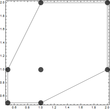
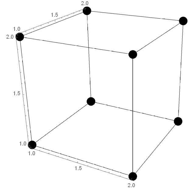
where for each 𝒙[a,b]3𝒙superscript𝑎𝑏3\boldsymbol{x}\in[a,b]^{3} we get 𝒕(𝒙)=(x2/x1,x3/x1)𝖳𝒕𝒙superscriptsubscript𝑥2subscript𝑥1subscript𝑥3subscript𝑥1𝖳\boldsymbol{t}(\boldsymbol{x})=(x_{2}/x_{1},x_{3}/x_{1})^{\sf T} as it is depicted in Figure 1 for, in specific, a=1𝑎1a=1 and b=2𝑏2b=2. In Gaffke et al. (2018) we showed that the support of a design is a subset of vertices of the ploytope. One notes that for each vertex 𝒗{(a,a,a)𝖳,(b,b,b)𝖳}𝒗superscript𝑎𝑎𝑎𝖳superscript𝑏𝑏𝑏𝖳\boldsymbol{v}\in\{(a,a,a)^{\sf T},(b,b,b)^{\sf T}\} we get 𝒕(𝒗)=(1,1)𝖳𝒕𝒗superscript11𝖳\boldsymbol{t}(\boldsymbol{v})=(1,1)^{\sf T} which lies in the interior of the convex hull above, i.e., (1,1)𝖳superscript11𝖳(1,1)^{\sf T} is a proper convex combination of the vertices of the polytope. Thus this reduction on the vertices implies that both vertices (a,a,a)𝖳superscript𝑎𝑎𝑎𝖳(a,a,a)^{\sf T} and (b,b,b)𝖳superscript𝑏𝑏𝑏𝖳(b,b,b)^{\sf T} of the hupercube [a,b]3superscript𝑎𝑏3[a,b]^{3} are out of consideration as support points of any optimal design.
Refer to caption
(a) The experimental region 𝒳=[1,2]3𝒳superscript123\mathcal{X}={[}1,2{]}^{3}.
Refer to caption
(b) The transformed experimental region Conv{(1/2,1/2)𝖳,(1/2,1)𝖳,(1,1/2)𝖳,(2,1)𝖳,(1,2)𝖳,(2,2)𝖳}Convsuperscript1212𝖳superscript121𝖳superscript112𝖳superscript21𝖳superscript12𝖳superscript22𝖳{\rm Conv}\bigl{\{}(1/2,1/2)^{\sf T},(1/2,1)^{\sf T},(1,1/2)^{\sf T},(2,1)^{\sf T},(1,2)^{\sf T},(2,2)^{\sf T}\bigr{\}}. The interior point is (1,1)𝖳superscript11𝖳(1,1)^{\sf T} which represents the original points (1,1,1)𝖳superscript111𝖳(1,1,1)^{\sf T} and (2,2,2)𝖳superscript222𝖳(2,2,2)^{\sf T} in [1,2]3superscript123{[}1,2{]}^{3}.
Figure 1:

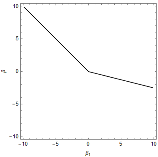
Let us concentrate on the experimental region 𝒳=[1,2]3𝒳superscript123\mathcal{X}=[1,2]^{3}. The linear predictor of a three-factor gamma model is given by η(𝒙,𝜷)=β1x1+β2x2+β3x3𝜂𝒙𝜷subscript𝛽1subscript𝑥1subscript𝛽2subscript𝑥2subscript𝛽3subscript𝑥3\eta(\boldsymbol{x},\boldsymbol{\beta})=\beta_{1}x_{1}+\beta_{2}x_{2}+\beta_{3}x_{3}. Assume that β2=β3=βsubscript𝛽2subscript𝛽3𝛽\beta_{2}=\beta_{3}=\beta, so the set of all parameter points under condition (2.5), i.e., β1x1+β2x2+β3x3>0subscript𝛽1subscript𝑥1subscript𝛽2subscript𝑥2subscript𝛽3subscript𝑥30\beta_{1}x_{1}+\beta_{2}x_{2}+\beta_{3}x_{3}>0 for all 𝒙=(x1,x2,x3)𝖳𝒳𝒙superscriptsubscript𝑥1subscript𝑥2subscript𝑥3𝖳𝒳\boldsymbol{x}=(x_{1},x_{2},x_{3})^{\sf T}\in\mathcal{X} is characterized by

β10,β>β1 or β1>0,β>14β1formulae-sequenceformulae-sequencesubscript𝛽10𝛽subscript𝛽1 or subscript𝛽10𝛽14subscript𝛽1\beta_{1}\leq 0,\,\beta>-\beta_{1}\,\mbox{ or }\,\beta_{1}>0,\,\beta>-\frac{1}{4}\beta_{1}

which is shown by Panel (a) of Figure 2.

Let the vertices of 𝒳=[1,2]3𝒳superscript123\mathcal{X}=[1,2]^{3} be denoted by 𝒗1=(1,1,1)𝖳subscript𝒗1superscript111𝖳\boldsymbol{v}_{1}=\big{(}1,1,1\big{)}^{\sf T}, 𝒗2=(2,1,1)𝖳subscript𝒗2superscript211𝖳\boldsymbol{v}_{2}=\big{(}2,1,1\big{)}^{\sf T}, 𝒗3=(1,2,1)𝖳subscript𝒗3superscript121𝖳\boldsymbol{v}_{3}=\big{(}1,2,1\big{)}^{\sf T}, 𝒗4=(1,1,2)𝖳subscript𝒗4superscript112𝖳\boldsymbol{v}_{4}=\big{(}1,1,2\big{)}^{\sf T}, 𝒗5=(1,2,2)𝖳subscript𝒗5superscript122𝖳\boldsymbol{v}_{5}=\big{(}1,2,2\big{)}^{\sf T}, 𝒗6=(2,1,2)𝖳subscript𝒗6superscript212𝖳\boldsymbol{v}_{6}=\big{(}2,1,2\big{)}^{\sf T}, 𝒗7=(2,2,1)𝖳subscript𝒗7superscript221𝖳\boldsymbol{v}_{7}=\big{(}2,2,1\big{)}^{\sf T}, 𝒗8=(2,2,2)𝖳subscript𝒗8superscript222𝖳\boldsymbol{v}_{8}=\big{(}2,2,2\big{)}^{\sf T} with intensities ui=u(𝒗i,𝜷),i=1,,νformulae-sequencesubscript𝑢𝑖𝑢subscript𝒗𝑖𝜷𝑖1𝜈u_{i}=u(\boldsymbol{v}_{i},\boldsymbol{\beta}),\,i=1,\dots,\nu. Actually, the region shown in Figure 2 is the parameter space of 𝜷=(β1,β2,β3)𝖳𝜷superscriptsubscript𝛽1subscript𝛽2subscript𝛽3𝖳\boldsymbol{\beta}=(\beta_{1},\beta_{2},\beta_{3})^{\sf T} only when β2=β3subscript𝛽2subscript𝛽3\beta_{2}=\beta_{3}. We aim at finding locally D-optimal designs at a given parameter point in that space. The expression “ optimality subregion” will be used to refer to a subset of parameter points where saturated designs or non-saturated designs with similar support are locally D-optimal.

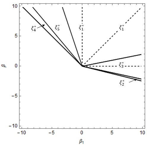
In the next theorem we introduce the locally D-optimal designs on respective optimality subregions. Table 1 presents the order of the intensities in all optimality subregions and the corresponding D-optimal designs. The intensities for both vertices 𝒗1subscript𝒗1\boldsymbol{v}_{1} and 𝒗8subscript𝒗8\boldsymbol{v}_{8} are ignored due to the reduction (cp. Remark 6). It is noted that on each subregion the vertices of highest intensities perform mostly as a support of the corresponding D-optimal design. In particular, analytic solution of the locally D-optimal designs of type ξ5superscriptsubscript𝜉5\xi_{5}^{*} at a point 𝜷𝜷\boldsymbol{\beta} from the subregion 3β1<β<65β13subscript𝛽1𝛽65subscript𝛽1-3\beta_{1}<\beta<-\frac{6}{5}\beta_{1},   β1<0subscript𝛽10\beta_{1}<0 cannot be developed so that numerical results are to be derived (cp. Remark 7).

Subregions          Intensities order          D-optimal design
β>0𝛽0\beta>0, β1=0subscript𝛽10\beta_{1}=0 u2>u3=u4=u6=u7>u5subscript𝑢2subscript𝑢3subscript𝑢4subscript𝑢6subscript𝑢7subscript𝑢5u_{2}>u_{3}=u_{4}=u_{6}=u_{7}>u_{5}           ξ1superscriptsubscript𝜉1\xi_{1}^{*}
β3β1𝛽3subscript𝛽1\beta\geq-3\beta_{1},  β1<0subscript𝛽10\beta_{1}<0 u2>u6=u7u3=u4>u5subscript𝑢2subscript𝑢6subscript𝑢7subscript𝑢3subscript𝑢4subscript𝑢5u_{2}>u_{6}=u_{7}\approx u_{3}=u_{4}>u_{5}           ξ1superscriptsubscript𝜉1\xi_{1}^{*}
β>15β1𝛽15subscript𝛽1\beta>\frac{1}{5}\beta_{1},  β1>0subscript𝛽10\beta_{1}>0 u2>u3=u4>u6=u7>u5subscript𝑢2subscript𝑢3subscript𝑢4subscript𝑢6subscript𝑢7subscript𝑢5u_{2}>u_{3}=u_{4}>u_{6}=u_{7}>u_{5}           ξ1superscriptsubscript𝜉1\xi_{1}^{*}
14β1<β523β114subscript𝛽1𝛽523subscript𝛽1-\frac{1}{4}\beta_{1}<\beta\leq-\frac{5}{23}\beta_{1},  β1>0subscript𝛽10\beta_{1}>0 u5>u3=u4>u6=u7>u2subscript𝑢5subscript𝑢3subscript𝑢4subscript𝑢6subscript𝑢7subscript𝑢2u_{5}>u_{3}=u_{4}>u_{6}=u_{7}>u_{2}           ξ2superscriptsubscript𝜉2\xi_{2}^{*}
523β1<β<15β1523subscript𝛽1𝛽15subscript𝛽1-\frac{5}{23}\beta_{1}<\beta<\frac{1}{5}\beta_{1},  β1>0subscript𝛽10\beta_{1}>0 u3=u4u5>u2u6=u7subscript𝑢3subscript𝑢4subscript𝑢5subscript𝑢2subscript𝑢6subscript𝑢7u_{3}=u_{4}\geq u_{5}>u_{2}\geq u_{6}=u_{7}           ξ3superscriptsubscript𝜉3\xi_{3}^{*}
β1<β65β1subscript𝛽1𝛽65subscript𝛽1-\beta_{1}<\beta\leq-\frac{6}{5}\beta_{1},  β1<0subscript𝛽10\beta_{1}<0 u2>u6=u7>u3=u4>u5subscript𝑢2subscript𝑢6subscript𝑢7subscript𝑢3subscript𝑢4subscript𝑢5u_{2}>u_{6}=u_{7}>u_{3}=u_{4}>u_{5}           ξ4superscriptsubscript𝜉4\xi_{4}^{*}
3β1<β<65β13subscript𝛽1𝛽65subscript𝛽1-3\beta_{1}<\beta<-\frac{6}{5}\beta_{1},   β1<0subscript𝛽10\beta_{1}<0 u2>u6=u7>u3=u4>u5subscript𝑢2subscript𝑢6subscript𝑢7subscript𝑢3subscript𝑢4subscript𝑢5u_{2}>u_{6}=u_{7}>u_{3}=u_{4}>u_{5}           ξ5superscriptsubscript𝜉5\xi_{5}^{*}
Table 1: The order of intensity values according to subregions correspond to D-optimal designs
Refer to caption
(a)
Refer to caption
(b)
Figure 2: Panel (a): The parameter space of 𝜷=(β1,β2,β3)𝖳𝜷superscriptsubscript𝛽1subscript𝛽2subscript𝛽3𝖳\boldsymbol{\beta}=(\beta_{1},\beta_{2},\beta_{3})^{\sf T} such that β2=β3=βsubscript𝛽2subscript𝛽3𝛽\beta_{2}=\beta_{3}=\beta.
Panel (b): Dependence of locally D-optimal designs from Theorem 3.3 on 𝜷=(β1,β2,β3)𝖳𝜷superscriptsubscript𝛽1subscript𝛽2subscript𝛽3𝖳\boldsymbol{\beta}=(\beta_{1},\beta_{2},\beta_{3})^{\sf T} such that β2=β3=βsubscript𝛽2subscript𝛽3𝛽\,\beta_{2}=\beta_{3}=\beta. The dashed lines are; diagonal: β=β1𝛽subscript𝛽1\beta=\beta_{1}, vertical: β1=0subscript𝛽10\beta_{1}=0, horizontal: β=0𝛽0\beta=0.
Theorem 3.3.

Consider the experimental region 𝒳=[1,2]3𝒳superscript123\mathcal{X}=[1,2]^{3}. Let a parameter point 𝛃=(β1,β2,β3)𝖳𝛃superscriptsubscript𝛽1subscript𝛽2subscript𝛽3𝖳\boldsymbol{\beta}=(\beta_{1},\beta_{2},\beta_{3})^{\sf T} be given such that β2=β3=βsubscript𝛽2subscript𝛽3𝛽\beta_{2}=\beta_{3}=\beta  with   β>β1𝛽subscript𝛽1\beta>-\beta_{1}  if  β10subscript𝛽10\beta_{1}\leq 0  or   β>14β1𝛽14subscript𝛽1\beta>-\frac{1}{4}\beta_{1}  if  β1>0subscript𝛽10\beta_{1}>0. Then the following designs are locally D-optimal (at 𝛃𝛃\boldsymbol{\beta}).

  1. (i)

    If    β>0𝛽0\beta>0, β1=0subscript𝛽10\beta_{1}=0   or   β3β1𝛽3subscript𝛽1\beta\geq-3\beta_{1}, β1<0subscript𝛽10\beta_{1}<0   or    β>15β1𝛽15subscript𝛽1\beta>\frac{1}{5}\beta_{1}, β1>0subscript𝛽10\beta_{1}>0 then

    ξ1=(𝒗2𝒗3𝒗4131313).superscriptsubscript𝜉1subscript𝒗2subscript𝒗3subscript𝒗4131313\displaystyle\xi_{1}^{*}=\left(\begin{array}[]{ccc}\boldsymbol{v}_{2}&\boldsymbol{v}_{3}&\boldsymbol{v}_{4}\\[2.15277pt] \frac{1}{3}&\frac{1}{3}&\frac{1}{3}\end{array}\right).
  2. (ii)

    If   14β1<β523β114subscript𝛽1𝛽523subscript𝛽1-\frac{1}{4}\beta_{1}<\beta\leq-\frac{5}{23}\beta_{1},  β1>0subscript𝛽10\beta_{1}>0 then

    ξ2=(𝒗3𝒗4𝒗5131313).superscriptsubscript𝜉2subscript𝒗3subscript𝒗4subscript𝒗5131313\displaystyle\xi_{2}^{*}=\left(\begin{array}[]{ccc}\boldsymbol{v}_{3}&\boldsymbol{v}_{4}&\boldsymbol{v}_{5}\\[2.15277pt] \frac{1}{3}&\frac{1}{3}&\frac{1}{3}\end{array}\right).
  3. (iii)

    If 523β1<β<15β1523subscript𝛽1𝛽15subscript𝛽1-\frac{5}{23}\beta_{1}<\beta<\frac{1}{5}\beta_{1},  β1>0subscript𝛽10\beta_{1}>0 then

    ξ3=(𝒗2𝒗3𝒗4𝒗5ω1ω2ω3ω4).superscriptsubscript𝜉3subscript𝒗2subscript𝒗3subscript𝒗4subscript𝒗5superscriptsubscript𝜔1superscriptsubscript𝜔2superscriptsubscript𝜔3superscriptsubscript𝜔4\displaystyle\xi_{3}^{*}=\left(\begin{array}[]{cccc}\boldsymbol{v}_{2}&\boldsymbol{v}_{3}&\boldsymbol{v}_{4}&\boldsymbol{v}_{5}\\[2.15277pt] \omega_{1}^{*}&\omega_{2}^{*}&\omega_{3}^{*}&\omega_{4}^{*}\end{array}\right).

    where

    ω1=5+23γ16(1+4γ),ω2=ω3=9(1+3γ)232(1+γ)(1+4γ),ω4=1γ20γ28(1+γ)(1+4γ),γ=ββ1.formulae-sequenceformulae-sequencesuperscriptsubscript𝜔1523𝛾1614𝛾superscriptsubscript𝜔2superscriptsubscript𝜔39superscript13𝛾2321𝛾14𝛾formulae-sequencesuperscriptsubscript𝜔41𝛾20superscript𝛾281𝛾14𝛾𝛾𝛽subscript𝛽1\omega_{1}^{*}=\frac{5+23\,\gamma}{16\,(1+4\,\gamma)},\,\,\omega_{2}^{*}=\omega_{3}^{*}=\frac{9\,(1+3\gamma)^{2}}{32\,(1+\gamma)(1+4\,\gamma)},\,\,\omega_{4}^{*}=\frac{1-\gamma-20\,\gamma^{2}}{8\,(1+\gamma)(1+4\,\gamma)},\,\,\gamma=\frac{\beta}{\beta_{1}}.
  4. (iv)

    If β1<β65β1subscript𝛽1𝛽65subscript𝛽1-\beta_{1}<\beta\leq-\frac{6}{5}\beta_{1},  β1<0subscript𝛽10\beta_{1}<0 then

    ξ4=(𝒗2𝒗6𝒗7131313).superscriptsubscript𝜉4subscript𝒗2subscript𝒗6subscript𝒗7131313\displaystyle\xi_{4}^{*}=\left(\begin{array}[]{ccc}\boldsymbol{v}_{2}&\boldsymbol{v}_{6}&\boldsymbol{v}_{7}\\[2.15277pt] \frac{1}{3}&\frac{1}{3}&\frac{1}{3}\end{array}\right).
Proof.

The proof is obtained by making use of the condition of the Equivalence Theorem (Theorem 2.1, part (a)). So that we develop a system of feasible inequalities evaluated at the vertices 𝒗isubscript𝒗𝑖\boldsymbol{v}_{i} for all (1i8)1𝑖8(1\leq i\leq 8). For simplicity in computations when β10subscript𝛽10\beta_{1}\neq 0 we utilize the ratio γ=β/β1𝛾𝛽subscript𝛽1\gamma=\beta/\beta_{1} of which the range is given by (,1)(14,)114(-\infty,-1)\cup(-\frac{1}{4},\infty). It turned out that some inequalities are equivalent and thus a resulted system is reduced to an equivalent system of a few inequalities. The intersection of the set of solutions of each system with the range of γ𝛾\gamma leads to the optimality condition (subregion) of the corresponding optimal design. Note that u1=β12(1+2γ)2subscript𝑢1superscriptsubscript𝛽12superscript12𝛾2u_{1}=\beta_{1}^{-2}\big{(}1\,+2\,\gamma\big{)}^{-2}, u2=β12(2+2γ)2subscript𝑢2superscriptsubscript𝛽12superscript22𝛾2u_{2}=\beta_{1}^{-2}\big{(}2\,+2\,\gamma\big{)}^{-2}, u3=u4=β12(1+3γ)2subscript𝑢3subscript𝑢4superscriptsubscript𝛽12superscript13𝛾2u_{3}=u_{4}=\beta_{1}^{-2}\big{(}1+3\,\gamma\big{)}^{-2}, u5=β12(1+4γ)2subscript𝑢5superscriptsubscript𝛽12superscript14𝛾2u_{5}=\beta_{1}^{-2}\big{(}1+4\,\gamma\big{)}^{-2}, u6=u7=β12(2+3γ)2subscript𝑢6subscript𝑢7superscriptsubscript𝛽12superscript23𝛾2u_{6}=u_{7}=\beta_{1}^{-2}\big{(}2+3\,\gamma\big{)}^{-2}, u8=β12(2+4γ)2subscript𝑢8superscriptsubscript𝛽12superscript24𝛾2u_{8}=\beta_{1}^{-2}\big{(}2+4\,\gamma\big{)}^{-2}.
(i𝑖i) The 3×3333\times 3 design matrix 𝑭=[𝒗2,𝒗3,𝒗4]𝖳𝑭superscriptsubscript𝒗2subscript𝒗3subscript𝒗4𝖳\boldsymbol{F}=[\boldsymbol{v}_{2},\boldsymbol{v}_{3},\boldsymbol{v}_{4}]^{\sf T} is given by

𝑭=(211121112) with 𝑭1=(341414143414141434) and weight matrix 𝑽=diag(u2,u3,u4).𝑭211missing-subexpression121missing-subexpression112 with superscript𝑭1341414missing-subexpression143414missing-subexpression141434 and weight matrix 𝑽diagsubscript𝑢2subscript𝑢3subscript𝑢4\displaystyle\boldsymbol{F}=\left(\begin{array}[]{ccc}2&1&1\\ \vskip 6.0pt plus 2.0pt minus 2.0pt\cr 1&2&1\\ \vskip 6.0pt plus 2.0pt minus 2.0pt\cr 1&1&2\\ \vskip 6.0pt plus 2.0pt minus 2.0pt\cr\end{array}\right)\,\,\mbox{ with }\,\,\boldsymbol{F}^{-1}=\left(\begin{array}[]{rrr}\frac{3}{4}&-\frac{1}{4}&-\frac{1}{4}\\ \vskip 6.0pt plus 2.0pt minus 2.0pt\cr-\frac{1}{4}&\frac{3}{4}&-\frac{1}{4}\\ \vskip 6.0pt plus 2.0pt minus 2.0pt\cr-\frac{1}{4}&-\frac{1}{4}&\frac{3}{4}\\ \vskip 6.0pt plus 2.0pt minus 2.0pt\cr\end{array}\right)\,\,\mbox{ and weight matrix }\boldsymbol{V}=\mathrm{diag}\big{(}u_{2},u_{3},u_{4}\big{)}.

Hence, the condition of The Equivalence Theorem is given by

𝒇𝖳(𝒙)𝑭1𝑽1(𝑭𝖳)1𝒇(𝒙)(β1x1+β2x2+β3x3)2𝒙{1,2}3.formulae-sequencesuperscript𝒇𝖳𝒙superscript𝑭1superscript𝑽1superscriptsuperscript𝑭𝖳1𝒇𝒙superscriptsubscript𝛽1subscript𝑥1subscript𝛽2subscript𝑥2subscript𝛽3subscript𝑥32for-all𝒙superscript123\displaystyle\boldsymbol{f}^{\sf T}(\boldsymbol{x})\boldsymbol{F}^{-1}\boldsymbol{V}^{-1}\big{(}\boldsymbol{F}^{\sf T}\big{)}^{-1}\boldsymbol{f}(\boldsymbol{x})\leq\big{(}\beta_{1}x_{1}+\beta_{2}x_{2}+\beta_{3}x_{3}\big{)}^{2}\,\,\,\,\,\,\forall\boldsymbol{x}\in\{1,2\}^{3}. (3.12)

For case β>0𝛽0\beta>0, β1=0subscript𝛽10\beta_{1}=0, condition (3.12) is equivalent to

4(3x1(x2+x3))2+9((3x2(x1+x3))2+(3x3(x1+x2))2)16(x2+x3)2𝒙{1,2}3,4superscript3subscript𝑥1subscript𝑥2subscript𝑥329superscript3subscript𝑥2subscript𝑥1subscript𝑥32superscript3subscript𝑥3subscript𝑥1subscript𝑥2216superscriptsubscript𝑥2subscript𝑥32for-all𝒙superscript123\displaystyle 4\big{(}3x_{1}-(x_{2}+x_{3})\big{)}^{2}+9\bigl{(}\big{(}3x_{2}-(x_{1}+x_{3})\big{)}^{2}+\big{(}3x_{3}-(x_{1}+x_{2})\big{)}^{2}\bigr{)}\leq 16\big{(}x_{2}+x_{3}\big{)}^{2}\,\,\forall\boldsymbol{x}\in\{1,2\}^{3},

which is independent of β𝛽\beta and is satisfied by 𝒗isubscript𝒗𝑖\boldsymbol{v}_{i} for all (1i8)1𝑖8(1\leq i\leq 8) with equality holds for the support. For the other cases condition (3.12) is equivalent to

(3x1(x2+x3))2(2+2γ)2+((3x2(x1+x3))2\displaystyle\big{(}3x_{1}-(x_{2}+x_{3})\big{)}^{2}(2\,+2\,\gamma)^{2}+\bigl{(}\big{(}3x_{2}-(x_{1}+x_{3})\big{)}^{2}
+(3x3(x1+x2))2)(1+3γ)216(x1+γ(x2+x3))2𝒙{1,2}3.\displaystyle+\big{(}3x_{3}-(x_{1}+x_{2})\big{)}^{2}\bigr{)}(1+3\,\gamma\big{)}^{2}\leq 16\big{(}x_{1}+\gamma(x_{2}+x_{3})\big{)}^{2}\,\,\forall\boldsymbol{x}\in\{1,2\}^{3}. (3.13)

After some lengthy but straightforward calculations, the above inequalities reduce to

15γ2+2γ10 for 𝒗515superscript𝛾22𝛾10 for subscript𝒗5\displaystyle 15\gamma^{2}+2\gamma-1\geq 0\mbox{ for }\boldsymbol{v}_{5} (3.14)
3γ2+10γ+30 for 𝒗6 or 𝒗73superscript𝛾210𝛾30 for 𝒗6 or 𝒗7\displaystyle 3\gamma^{2}+10\gamma+3\geq 0\mbox{ for $\boldsymbol{v}_{6}$ or $\boldsymbol{v}_{7}$ } (3.15)

The l.h.s. of each of (3.14) and (3.15) above is a polynomial in γ𝛾\gamma of degree 2 and thus the sets of solutions are given by (,13][15,)1315(-\infty,-\frac{1}{3}]\cup[\frac{1}{5},\infty) and (,3][13,)313(-\infty,-3]\cup[-\frac{1}{3},\infty), respectively. Note that the interior bounds are the roots of the respective polynomials. Hence, by considering the intersection of both sets with the range of γ𝛾\gamma, the design ξ1superscriptsubscript𝜉1\xi_{1}^{*} is locally D-optimal if γ(,3][15,)𝛾315\gamma\in(-\infty,-3]\cup[\frac{1}{5},\infty) which is equivalent to the optimality subregion β3β1𝛽3subscript𝛽1\beta\geq-3\beta_{1}, β1<0subscript𝛽10\beta_{1}<0   or    β>15β1𝛽15subscript𝛽1\beta>\frac{1}{5}\beta_{1}, β1>0subscript𝛽10\beta_{1}>0 given in part (i𝑖i) of the theorem.
(ii𝑖𝑖ii) The 3×3333\times 3 design matrix 𝑭=[𝒗3,𝒗4,𝒗5]𝖳𝑭superscriptsubscript𝒗3subscript𝒗4subscript𝒗5𝖳\boldsymbol{F}=[\boldsymbol{v}_{3},\boldsymbol{v}_{4},\boldsymbol{v}_{5}]^{\sf T} is given by

𝑭=(121112122) with 𝑭1=(223011101) and weight matrix 𝑽=diag(u3,u4,u5).𝑭121missing-subexpression112missing-subexpression122 with superscript𝑭1223missing-subexpression011missing-subexpression101 and weight matrix 𝑽diagsubscript𝑢3subscript𝑢4subscript𝑢5\displaystyle\boldsymbol{F}=\left(\begin{array}[]{ccc}1&2&1\\ \vskip 6.0pt plus 2.0pt minus 2.0pt\cr 1&1&2\\ \vskip 6.0pt plus 2.0pt minus 2.0pt\cr 1&2&2\end{array}\right)\,\,\mbox{ with }\,\,\boldsymbol{F}^{-1}=\left(\begin{array}[]{rrr}2&2&-3\\ \vskip 6.0pt plus 2.0pt minus 2.0pt\cr 0&-1&1\\ \vskip 6.0pt plus 2.0pt minus 2.0pt\cr-1&0&1\end{array}\right)\,\,\mbox{ and weight matrix }\,\,\boldsymbol{V}=\mathrm{diag}\big{(}u_{3},u_{4},u_{5}\big{)}.

Hence, the condition of The Equivalence Theorem is equivalent to

((2x1x2)2+(2x1x3)2)(1+3γ)2+(x3+x23x1)2(1+4γ)2(x1+γ(x2+x3))2𝒙{1,2}3,superscript2subscript𝑥1subscript𝑥22superscript2subscript𝑥1subscript𝑥32superscript13𝛾2superscriptsubscript𝑥3subscript𝑥23subscript𝑥12superscript14𝛾2superscriptsubscript𝑥1𝛾subscript𝑥2subscript𝑥32for-all𝒙superscript123\displaystyle\big{(}\big{(}2\,x_{1}-x_{2}\big{)}^{2}+\big{(}2\,x_{1}-x_{3}\big{)}^{2}\big{)}\,\big{(}1+3\,\gamma\big{)}^{2}+\big{(}x_{3}+x_{2}-3\,x_{1}\big{)}^{2}\,\big{(}1+4\,\gamma\big{)}^{2}\leq\big{(}x_{1}+\gamma(x_{2}+x_{3})\big{)}^{2}\,\,\forall\boldsymbol{x}\in\{1,2\}^{3},

and also the above inequalities reduce to

69γ2+38γ+50 for 𝒗2 .69superscript𝛾238𝛾50 for 𝒗2 \displaystyle 69\gamma^{2}+38\gamma+5\leq 0\mbox{ for $\boldsymbol{v}_{2}$ }. (3.17)

Again, the set of solutions of the polynomial determined by the l.h.s. of inequality (3.17) is given by [13,523]13523[-\frac{1}{3},-\frac{5}{23}]. By considering the intersection with the range of γ𝛾\gamma, the design ξ2superscriptsubscript𝜉2\xi_{2}^{*} is locally D-optimal if γ(14,523]𝛾14523\gamma\in(-\frac{1}{4},-\frac{5}{23}]
(iii𝑖𝑖𝑖iii) Consider design ξ3superscriptsubscript𝜉3\xi_{3}^{*}. Note that ω1>0superscriptsubscript𝜔10\omega_{1}^{*}>0 for all γ>5/23𝛾523\gamma>-5/23, ω2>0superscriptsubscript𝜔20\omega_{2}^{*}>0 for all γ𝛾\gamma\in\mathbb{R} and ω4>0superscriptsubscript𝜔40\omega_{4}^{*}>0 for all γ(14,15)𝛾1415\gamma\in(-\frac{1}{4},\frac{1}{5}), and thus it is obvious that ω1,ω2,ω4superscriptsubscript𝜔1superscriptsubscript𝜔2superscriptsubscript𝜔4\omega_{1}^{*},\omega_{2}^{*},\omega_{4}^{*} are positive over (523,15)52315(-\frac{5}{23},\frac{1}{5}) and i=14ωi=1superscriptsubscript𝑖14superscriptsubscript𝜔𝑖1\sum_{i=1}^{4}\omega_{i}^{*}=1. The 4×3434\times 3 design matrix is given by 𝑭=[𝒗2,𝒗3,𝒗4,𝒗5]𝖳𝑭superscriptsubscript𝒗2subscript𝒗3subscript𝒗4subscript𝒗5𝖳\boldsymbol{F}=[\boldsymbol{v}_{2},\boldsymbol{v}_{3},\boldsymbol{v}_{4},\boldsymbol{v}_{5}]^{\sf T} with weight matrix 𝑽=diag(s2,s3,s4,s5)𝑽diagsubscript𝑠2subscript𝑠3subscript𝑠4subscript𝑠5\boldsymbol{V}=\mathrm{diag}\big{(}s_{2},s_{3},s_{4},s_{5}\big{)} where si=ωiui,i=2,3,4,5formulae-sequencesubscript𝑠𝑖superscriptsubscript𝜔𝑖subscript𝑢𝑖𝑖2345s_{i}=\omega_{i}^{*}u_{i},i=2,3,4,5 and s3=s4subscript𝑠3subscript𝑠4s_{3}=s_{4}. The information matrix is given by

𝑴(ξ3,𝜷)=(4s2+2s3+s52s2+3s3+2s52s2+3s3+2s52s2+3s2+2s5s2+5s3+4s5s2+4s3+4s52s2+3s3+2s5s2+4s3+4s4s2+5s3+4s5)𝑴superscriptsubscript𝜉3𝜷4subscript𝑠22subscript𝑠3subscript𝑠52subscript𝑠23subscript𝑠32subscript𝑠52subscript𝑠23subscript𝑠32subscript𝑠5missing-subexpression2subscript𝑠23subscript𝑠22subscript𝑠5subscript𝑠25subscript𝑠34subscript𝑠5subscript𝑠24subscript𝑠34subscript𝑠5missing-subexpression2subscript𝑠23subscript𝑠32subscript𝑠5subscript𝑠24subscript𝑠34subscript𝑠4subscript𝑠25subscript𝑠34subscript𝑠5\displaystyle\boldsymbol{M}\bigl{(}\xi_{3}^{*},\boldsymbol{\beta}\bigr{)}=\left(\begin{array}[]{ccc}4\,s_{2}+2\,s_{3}+s_{5}&2\,s_{2}+3\,s_{3}+2\,s_{5}&2\,s_{2}+3\,s_{3}+2\,s_{5}\\ \vskip 6.0pt plus 2.0pt minus 2.0pt\cr 2\,s_{2}+3\,s_{2}+2\,s_{5}&s_{2}+5\,s_{3}+4\,s_{5}&s_{2}+4\,s_{3}+4\,s_{5}\\ \vskip 6.0pt plus 2.0pt minus 2.0pt\cr 2\,s_{2}+3\,s_{3}+2\,s_{5}&s_{2}+4\,s_{3}+4\,s_{4}&s_{2}+5\,s_{3}+4\,s_{5}\end{array}\right)

and one calculates det𝑴(ξ3,𝜷)=16s2s32+18s2s3s5+s32s5𝑴superscriptsubscript𝜉3𝜷16subscript𝑠2superscriptsubscript𝑠3218subscript𝑠2subscript𝑠3subscript𝑠5superscriptsubscript𝑠32subscript𝑠5\det\boldsymbol{M}\bigl{(}\xi_{3}^{*},\boldsymbol{\beta}\bigr{)}=16\,s_{2}\,s_{3}^{2}+18\,s_{2}\,s_{3}\,s_{5}+s_{3}^{2}s_{5}. Define the following quantities

c1=s3(2s2+9s3+8s5)16s2s32+18s2s3s5+s32s5,c2=s3(2s2+3s3+2s5)16s2s32+18s2s3s5+s32s5,formulae-sequencesubscript𝑐1subscript𝑠32subscript𝑠29subscript𝑠38subscript𝑠516subscript𝑠2superscriptsubscript𝑠3218subscript𝑠2subscript𝑠3subscript𝑠5superscriptsubscript𝑠32subscript𝑠5subscript𝑐2subscript𝑠32subscript𝑠23subscript𝑠32subscript𝑠516subscript𝑠2superscriptsubscript𝑠3218subscript𝑠2subscript𝑠3subscript𝑠5superscriptsubscript𝑠32subscript𝑠5\displaystyle c_{1}=\frac{s_{3}(2\,s_{2}+9\,s_{3}+8\,s_{5})}{16\,s_{2}\,s_{3}^{2}+18\,s_{2}\,s_{3}\,s_{5}+s_{3}^{2}s_{5}},\,\,c_{2}=\frac{-s_{3}(2\,s_{2}+3\,s_{3}+2\,s_{5})}{16\,s_{2}\,s_{3}^{2}+18\,s_{2}\,s_{3}\,s_{5}+s_{3}^{2}s_{5}},
c3=10s2s3+9s2s5+s32+s3s516s2s32+18s2s3s5+s32s5,c4=6s2s3+9s2s5s3216s2s32+18s2s3s5+s32s5.formulae-sequencesubscript𝑐310subscript𝑠2subscript𝑠39subscript𝑠2subscript𝑠5superscriptsubscript𝑠32subscript𝑠3subscript𝑠516subscript𝑠2superscriptsubscript𝑠3218subscript𝑠2subscript𝑠3subscript𝑠5superscriptsubscript𝑠32subscript𝑠5subscript𝑐46subscript𝑠2subscript𝑠39subscript𝑠2subscript𝑠5superscriptsubscript𝑠3216subscript𝑠2superscriptsubscript𝑠3218subscript𝑠2subscript𝑠3subscript𝑠5superscriptsubscript𝑠32subscript𝑠5\displaystyle c_{3}=\frac{10\,s_{2}\,s_{3}+9\,s_{2}\,s_{5}+s_{3}^{2}+s_{3}\,s_{5}}{16\,s_{2}\,s_{3}^{2}+18\,s_{2}\,s_{3}\,s_{5}+s_{3}^{2}s_{5}},\,\,c_{4}=\frac{-6\,s_{2}\,s_{3}+9\,s_{2}\,s_{5}-s_{3}^{2}}{16\,s_{2}\,s_{3}^{2}+18\,s_{2}\,s_{3}\,s_{5}+s_{3}^{2}s_{5}}.
The inverse of the information matrix is given by
𝑴1(ξ3,𝜷)=(c1c2c2c2c3c4c2c4c3). Hence, the condition of The Equivalence Theoremformulae-sequencesuperscript𝑴1superscriptsubscript𝜉3𝜷subscript𝑐1subscript𝑐2subscript𝑐2missing-subexpressionmissing-subexpressionmissing-subexpressionsubscript𝑐2subscript𝑐3subscript𝑐4missing-subexpressionmissing-subexpressionmissing-subexpressionsubscript𝑐2subscript𝑐4subscript𝑐3 Hence, the condition of The Equivalence Theorem\displaystyle\boldsymbol{M}^{-1}\bigl{(}\xi_{3}^{*},\boldsymbol{\beta}\bigr{)}=\left(\begin{array}[]{ccc}c_{1}&c_{2}&c_{2}\\ \vskip 6.0pt plus 2.0pt minus 2.0pt\cr c_{2}&c_{3}&c_{4}\\ \vskip 6.0pt plus 2.0pt minus 2.0pt\cr c_{2}&c_{4}&c_{3}\end{array}\right).\,\,\mbox{ Hence, the condition of The Equivalence Theorem}
is equivalent to
c1x12+c3(x22+x32)+2c2(x1x2+x1x3)+2c4x2x33(x1+γ(x2+x3))2𝒙{1,2}3subscript𝑐1superscriptsubscript𝑥12subscript𝑐3superscriptsubscript𝑥22superscriptsubscript𝑥322subscript𝑐2subscript𝑥1subscript𝑥2subscript𝑥1subscript𝑥32subscript𝑐4subscript𝑥2subscript𝑥33superscriptsubscript𝑥1𝛾subscript𝑥2subscript𝑥32for-all𝒙superscript123\displaystyle c_{1}\,x_{1}^{2}+c_{3}\,(x_{2}^{2}+x_{3}^{2})+2\,c_{2}\,(x_{1}\,x_{2}+x_{1}\,x_{3})+2\,c_{4}\,x_{2}\,x_{3}\leq 3\,\big{(}x_{1}+\gamma\,(x_{2}+x_{3})\big{)}^{2}\,\,\forall\,\,\boldsymbol{x}\in\{1,2\}^{3}
which is equivalent to the following system of inequalities
c1+4c2+2c3+2c43(1+2γ)2 for 𝒗1 or 𝒗8subscript𝑐14subscript𝑐22subscript𝑐32subscript𝑐43superscript12𝛾2 for 𝒗1 or 𝒗8\displaystyle c_{1}+4c_{2}+2c_{3}+2c_{4}\leq 3\left(1+2\gamma\right)^{2}\mbox{ for $\boldsymbol{v}_{1}$ or $\boldsymbol{v}_{8}$ }
4c1+12c2+5c3+4c43(2+3γ)2 for 𝒗6 or 𝒗74subscript𝑐112subscript𝑐25subscript𝑐34subscript𝑐43superscript23𝛾2 for 𝒗6 or 𝒗7\displaystyle 4c_{1}+12c_{2}+5c_{3}+4c_{4}\leq 3\left(2+3\gamma\right)^{2}\mbox{ for $\boldsymbol{v}_{6}$ or $\boldsymbol{v}_{7}$ }

However, due to the complexity of the system above we employed computer algebra using Wolfram Mathematica 11.3 (see Wolfram Research ) to obtain the solution for γ𝛾\gamma.
(iv𝑖𝑣iv) The 3×3333\times 3 design matrix 𝑭=[𝒗2,𝒗6,𝒗7]𝖳𝑭superscriptsubscript𝒗2subscript𝒗6subscript𝒗7𝖳\boldsymbol{F}=[\boldsymbol{v}_{2},\boldsymbol{v}_{6},\boldsymbol{v}_{7}]^{\sf T} is given by

𝑭=(211212221) with 𝑭1=(32121212011210) and weight matrix 𝑽=diag(u2,u6,u7).𝑭211missing-subexpression212missing-subexpression221 with superscript𝑭1321212missing-subexpression1201missing-subexpression1210 and weight matrix 𝑽diagsubscript𝑢2subscript𝑢6subscript𝑢7\displaystyle\boldsymbol{F}=\left(\begin{array}[]{ccc}2&1&1\\ \vskip 6.0pt plus 2.0pt minus 2.0pt\cr 2&1&2\\ \vskip 6.0pt plus 2.0pt minus 2.0pt\cr 2&2&1\end{array}\right)\,\,\mbox{ with }\,\,\boldsymbol{F}^{-1}=\left(\begin{array}[]{rrr}\frac{3}{2}&-\frac{1}{2}&-\frac{1}{2}\\ \vskip 6.0pt plus 2.0pt minus 2.0pt\cr-\frac{1}{2}&0&1\\ \vskip 6.0pt plus 2.0pt minus 2.0pt\cr-\frac{1}{2}&1&0\end{array}\right)\,\,\mbox{ and weight matrix }\,\,\boldsymbol{V}=\mathrm{diag}\big{(}u_{2},u_{6},u_{7}\big{)}.

Hence, the condition of The Equivalence Theorem is equivalent to

((x2x12)2+(x3x12)2)(2+3γ)2+(3x12x2x3)2(2+2γ)2(x1+γ(x2+x3))2𝒙{1,2}3,superscriptsubscript𝑥2subscript𝑥122superscriptsubscript𝑥3subscript𝑥122superscript23𝛾2superscript3subscript𝑥12subscript𝑥2subscript𝑥32superscript22𝛾2superscriptsubscript𝑥1𝛾subscript𝑥2subscript𝑥32for-all𝒙superscript123\displaystyle\left(\left(x_{2}-\frac{x_{1}}{2}\right)^{2}+\left(x_{3}-\frac{x_{1}}{2}\right)^{2}\right)\left(2+3\gamma\right)^{2}+\left(\frac{3x_{1}}{2}-x_{2}-x_{3}\right)^{2}\left(2+2\gamma\right)^{2}\leq\big{(}x_{1}+\gamma(x_{2}+x_{3})\big{)}^{2}\,\,\forall\boldsymbol{x}\in\{1,2\}^{3},

and the above inequalities reduce to

90γ2+168γ+720 for 𝒗3 or 𝒗490superscript𝛾2168𝛾720 for 𝒗3 or 𝒗4\displaystyle 90\,\gamma^{2}+168\gamma+72\leq 0\mbox{ for $\boldsymbol{v}_{3}$ or $\boldsymbol{v}_{4}$} (3.21)
6γ2+16γ+80 for 𝒗86superscript𝛾216𝛾80 for 𝒗8\displaystyle 6\gamma^{2}+16\gamma+8\leq 0\mbox{ for $\boldsymbol{v}_{8}$ } (3.22)

In analogy to parts (i𝑖i) and (ii𝑖𝑖ii) the sets of solutions of (3.21) and (3.22) are given by [1.2,23]1.223[-1.2,-\frac{2}{3}] and [2,23]223[-2,-\frac{2}{3}], respectively where the interior bounds are the roots of the respective polynomials. Hence, by considering the intersection of both sets with the range of γ𝛾\gamma, the design ξ4superscriptsubscript𝜉4\xi_{4}^{*} is locally D-optimal if γ[1.2,1)𝛾1.21\gamma\in[-1.2,-1). ∎

In Panel (b) of Figure 2 the optimality subregions of ξ1superscriptsubscript𝜉1\xi_{1}^{*}, ξ2superscriptsubscript𝜉2\xi_{2}^{*}, ξ3superscriptsubscript𝜉3\xi_{3}^{*} and ξ4superscriptsubscript𝜉4\xi_{4}^{*} form Theorem 3.3 are depicted. Note that each design of ξ1superscriptsubscript𝜉1\xi_{1}^{*}, ξ2superscriptsubscript𝜉2\xi_{2}^{*} and ξ4superscriptsubscript𝜉4\xi_{4}^{*} denotes a single design whereas ξ3superscriptsubscript𝜉3\xi_{3}^{*} determines a certain type of designs with weights depend on the parameter values. A well known form of ξ3superscriptsubscript𝜉3\xi_{3}^{*} is obtained at β=(1/7)β1𝛽17subscript𝛽1\beta=(-1/7)\beta_{1} which represents the uniform design on the vertices 𝒗2,𝒗3,𝒗4,𝒗5subscript𝒗2subscript𝒗3subscript𝒗4subscript𝒗5\boldsymbol{v}_{2},\boldsymbol{v}_{3},\boldsymbol{v}_{4},\boldsymbol{v}_{5}. Additionally, along the horizontal dashed line, i.e., β=0𝛽0\beta=0, ξ3superscriptsubscript𝜉3\xi_{3}^{*} assigns the weights ω1=5/16,ω2=ω3=9/32,ω4=1/8formulae-sequenceformulae-sequencesuperscriptsubscript𝜔1516superscriptsubscript𝜔2superscriptsubscript𝜔3932superscriptsubscript𝜔418\omega_{1}^{*}=5/16,\omega_{2}^{*}=\omega_{3}^{*}=9/32,\omega_{4}^{*}=1/8 to 𝒗2,𝒗3,𝒗4,𝒗5subscript𝒗2subscript𝒗3subscript𝒗4subscript𝒗5\boldsymbol{v}_{2},\boldsymbol{v}_{3},\boldsymbol{v}_{4},\boldsymbol{v}_{5}, respectively. For equally size of parameters, i.e., β1=βsubscript𝛽1𝛽\beta_{1}=\beta the diagonal dashed line in Panel (b) represents a case where ξ1superscriptsubscript𝜉1\xi_{1}^{*} is D-optimal.

Remark 7.

Deriving a locally D-optimal design at a given parameter point from the subregion 3β1<β<65β13subscript𝛽1𝛽65subscript𝛽1-3\beta_{1}<\beta<-\frac{6}{5}\beta_{1},   β1<0subscript𝛽10\beta_{1}<0 is not available analytically. Therefore, employing the multiplicative algorithm (see Yu (2010) and Harman and Trnovská (2009)) in the software package R (see R Core Team (2018)) provides numerical solutions which show that the locally D-optimal design on that subregion is of form

ξ5=(𝒗2𝒗3𝒗4𝒗6𝒗7ω1ω2ω2ω3ω3)superscriptsubscript𝜉5subscript𝒗2subscript𝒗3subscript𝒗4subscript𝒗6subscript𝒗7superscriptsubscript𝜔1superscriptsubscript𝜔2superscriptsubscript𝜔2superscriptsubscript𝜔3superscriptsubscript𝜔3\displaystyle\xi_{5}^{*}=\left(\begin{array}[]{ccccc}\boldsymbol{v}_{2}&\boldsymbol{v}_{3}&\boldsymbol{v}_{4}&\boldsymbol{v}_{6}&\boldsymbol{v}_{7}\\[2.15277pt] \omega_{1}^{*}&\omega_{2}^{*}&\omega_{2}^{*}&\omega_{3}^{*}&\omega_{3}^{*}\end{array}\right)

which is supported by five vertices with weights may depend on 𝜷𝜷\boldsymbol{\beta}. The equal weights are due to the symmetry. Table 2 shows some numerical results in terms of the ratio γ=β/β1𝛾𝛽subscript𝛽1\gamma=\beta/\beta_{1} where γ(3,6/5)𝛾365\gamma\in(-3,-6/5) .

γ𝛾\,\,\,\,\,\gamma          𝒗2subscript𝒗2\boldsymbol{v}_{2}          𝒗3subscript𝒗3\boldsymbol{v}_{3}          𝒗4subscript𝒗4\boldsymbol{v}_{4}          𝒗6subscript𝒗6\boldsymbol{v}_{6}          𝒗7subscript𝒗7\boldsymbol{v}_{7}
2.92.9-2.9 0.3312 0.3285 0.3285 0.0059 0.0059
2.52.5-2.5 0.3225 0.3051 0.3051 0.0336 0.0336
22-2 0.3125 0.2604 0.2604 0.0833 0.0833
1.51.5-1.5 0.3125 0.1701 0.1701 0.1736 0.1736
1.231.23-1.23 0.3297 0.0325 0.0325 0.3027 0.3027
Table 2: D-optimal designs on 𝒳=[1,2]3𝒳superscript123\mathcal{X}=\left[1,2\right]^{3} at γ(3,6/5)𝛾365\gamma\in(-3,-6/5) where γ=β/β1𝛾𝛽subscript𝛽1\gamma=\beta/\beta_{1} and 3β1<β<65β13subscript𝛽1𝛽65subscript𝛽1-3\beta_{1}<\beta<-\frac{6}{5}\beta_{1},   β1<0subscript𝛽10\beta_{1}<0.

In general, for gamma models without intercept, finding optimal designs for a model with multiple factors, i.e., ν>3𝜈3\nu>3 is not an easy task. The optimal design given by part (i𝑖i) of Theorem 3.3 might be extended for arbitrary number of factors under sufficient and necessarily condition on the parameter points:

Theorem 3.4.

Consider the experimental region 𝒳=[a,b]ν,ν3, 0<a<bformulae-sequence𝒳superscript𝑎𝑏𝜈formulae-sequence𝜈3 0𝑎𝑏\mathcal{X}=\big{[}a,b\big{]}^{\nu},\nu\geq 3,\,0<a<b. Let 𝛃𝛃\boldsymbol{\beta} be a parameter point such that 𝐟𝖳(𝐱)𝛃>0superscript𝐟𝖳𝐱𝛃0\boldsymbol{f}^{\sf T}(\boldsymbol{x})\boldsymbol{\beta}>0 for all 𝐱𝒳𝐱𝒳\boldsymbol{x}\in\mathcal{X}. Define T(𝐱)=i=1νxi𝑇𝐱superscriptsubscript𝑖1𝜈subscript𝑥𝑖T(\boldsymbol{x})=\sum_{i=1}^{\nu}x_{i}, q=a(ν1)a+b𝑞𝑎𝜈1𝑎𝑏q=\frac{a}{(\nu-1)a+b} and cj=(ba)βj+ai=1νβisubscript𝑐𝑗𝑏𝑎subscript𝛽𝑗𝑎superscriptsubscript𝑖1𝜈subscript𝛽𝑖c_{j}=(b-a)\beta_{j}+a\sum_{i=1}^{\nu}\beta_{i} (1jν1𝑗𝜈1\leq j\leq\nu). Then the design ξsuperscript𝜉\xi^{*} which assigns equal weights ν1superscript𝜈1\nu^{-1} to the support

𝒙1=(b,a,,a)𝖳,𝒙2=(a,b,,a)𝖳,,𝒙ν=(a,a,,b)𝖳formulae-sequencesubscriptsuperscript𝒙1superscript𝑏𝑎𝑎𝖳formulae-sequencesubscriptsuperscript𝒙2superscript𝑎𝑏𝑎𝖳subscriptsuperscript𝒙𝜈superscript𝑎𝑎𝑏𝖳\boldsymbol{x}^{*}_{1}=\big{(}b,a,\dots,a\big{)}^{\sf T},\,\boldsymbol{x}^{*}_{2}=\big{(}a,b,\dots,a\big{)}^{\sf T},\,\dots\,,\,\boldsymbol{x}^{*}_{\nu}=\big{(}a,a,\dots,b\big{)}^{\sf T}

is locally D-optimal (at 𝛃𝛃\boldsymbol{\beta}) if and only if for all 𝐱=(x1,,xν)𝖳{a,b}ν𝐱superscriptsubscript𝑥1subscript𝑥𝜈𝖳superscript𝑎𝑏𝜈\boldsymbol{x}=(x_{1},\dots,x_{\nu})^{\sf T}\in\{a,b\}^{\nu}

j=1ν(xjqT(𝒙))2cj2(ba)2(j=1vβjxj)2.superscriptsubscript𝑗1𝜈superscriptsubscript𝑥𝑗𝑞𝑇𝒙2superscriptsubscript𝑐𝑗2superscript𝑏𝑎2superscriptsuperscriptsubscript𝑗1𝑣subscript𝛽𝑗subscript𝑥𝑗2\sum_{j=1}^{\nu}\big{(}x_{j}-qT(\boldsymbol{x})\big{)}^{2}c_{j}^{2}\leq(b-a)^{2}\big{(}\sum_{j=1}^{v}\beta_{j}x_{j}\big{)}^{2}. (3.24)
Proof.

Define the ν×ν𝜈𝜈\nu\times\nu design matrix 𝑭=[𝒇(𝒙1),,𝒇(𝒙ν)]𝖳𝑭superscript𝒇subscriptsuperscript𝒙1𝒇subscriptsuperscript𝒙𝜈𝖳\boldsymbol{F}=[\boldsymbol{f}(\boldsymbol{x}^{*}_{1}),\dots,\boldsymbol{f}(\boldsymbol{x}^{*}_{\nu})]^{\sf T}. Thus 𝑭=(ba)𝑰+a𝟏𝟏𝖳𝑭𝑏𝑎𝑰𝑎superscript11𝖳\boldsymbol{F}=(b-a)\boldsymbol{I}+a\boldsymbol{1}\boldsymbol{1}^{\sf T} and 𝑭1=1(ba)(𝑰q𝟏𝟏𝖳)superscript𝑭11𝑏𝑎𝑰𝑞superscript11𝖳\boldsymbol{F}^{-1}=\frac{1}{(b-a)}\left(\boldsymbol{I}-q\boldsymbol{1}\boldsymbol{1}^{\sf T}\right) where 𝑰𝑰\boldsymbol{I} is the ν×ν𝜈𝜈\nu\times\nu identity matrix and 𝟏1\boldsymbol{1} is a ν×1𝜈1\nu\times 1 vector of ones. The information matrix of ξsuperscript𝜉\xi^{*} is given by 𝑴(ξ,𝜷)=1ν𝑭𝖳𝑽𝑭𝑴superscript𝜉𝜷1𝜈superscript𝑭𝖳𝑽𝑭\boldsymbol{M}\bigl{(}\xi^{*},\boldsymbol{\beta}\bigr{)}=\frac{1}{\nu}\boldsymbol{F}^{\sf T}\boldsymbol{V}\boldsymbol{F} where 𝑽=diag(u(𝒙j,𝜷))j=1ν𝑽diagsuperscriptsubscript𝑢subscriptsuperscript𝒙𝑗𝜷𝑗1𝜈\boldsymbol{V}=\mathrm{diag}\Big{(}u(\boldsymbol{x}^{*}_{j},\boldsymbol{\beta})\Big{)}_{j=1}^{\nu} is the ν×ν𝜈𝜈\nu\times\nu weight matrix. Note that u(𝒙j,𝜷)=cj2𝑢subscriptsuperscript𝒙𝑗𝜷superscriptsubscript𝑐𝑗2u(\boldsymbol{x}^{*}_{j},\boldsymbol{\beta})=c_{j}^{-2}  for all  (1jν)1𝑗𝜈(1\leq j\leq\nu). Hence, the l.h.s. of the condition of the Equivalence Theorem (Theorem 2.1, part (a)) is equal to

(j=1vβjxj)2𝒇𝖳(𝒙)𝑴1(ξ,𝜷)𝒇(𝒙)=ν(j=1vβjxj)2𝒇𝖳(𝒙)𝑭1𝑽1𝑭1𝒇(𝒙)superscriptsuperscriptsubscript𝑗1𝑣subscript𝛽𝑗subscript𝑥𝑗2superscript𝒇𝖳𝒙superscript𝑴1superscript𝜉𝜷𝒇𝒙𝜈superscriptsuperscriptsubscript𝑗1𝑣subscript𝛽𝑗subscript𝑥𝑗2superscript𝒇𝖳𝒙superscript𝑭1superscript𝑽1superscript𝑭1𝒇𝒙\displaystyle\big{(}\sum_{j=1}^{v}\beta_{j}x_{j}\big{)}^{-2}\boldsymbol{f}^{\sf T}(\boldsymbol{x})\boldsymbol{M}^{-1}\bigl{(}\xi^{*},\boldsymbol{\beta}\bigr{)}\boldsymbol{f}(\boldsymbol{x})=\nu\big{(}\sum_{j=1}^{v}\beta_{j}x_{j}\big{)}^{-2}\boldsymbol{f}^{\sf T}(\boldsymbol{x})\boldsymbol{F}^{-1}\boldsymbol{V}^{-1}\boldsymbol{F}^{-1}\boldsymbol{f}(\boldsymbol{x})
=ν((ba)j=1vβjxj)2(𝒇𝖳(𝒙)qT(𝒙)𝟏𝖳)diag(cj2)j=1ν(𝒇(𝒙)qT(𝒙)𝟏)absent𝜈superscript𝑏𝑎superscriptsubscript𝑗1𝑣subscript𝛽𝑗subscript𝑥𝑗2superscript𝒇𝖳𝒙𝑞𝑇𝒙superscript1𝖳diagsuperscriptsubscriptsuperscriptsubscript𝑐𝑗2𝑗1𝜈𝒇𝒙𝑞𝑇𝒙1\displaystyle=\nu\big{(}(b-a)\sum_{j=1}^{v}\beta_{j}x_{j}\big{)}^{-2}\left(\boldsymbol{f}^{\sf T}(\boldsymbol{x})-qT(\boldsymbol{x})\boldsymbol{1}^{\sf T}\right)\mathrm{diag}\Big{(}c_{j}^{2}\Big{)}_{j=1}^{\nu}\left(\boldsymbol{f}(\boldsymbol{x})-qT(\boldsymbol{x})\boldsymbol{1}\right)
=ν((ba)j=1vβjxj)2j=1ν(xjqT(𝒙))2cj2.absent𝜈superscript𝑏𝑎superscriptsubscript𝑗1𝑣subscript𝛽𝑗subscript𝑥𝑗2superscriptsubscript𝑗1𝜈superscriptsubscript𝑥𝑗𝑞𝑇𝒙2superscriptsubscript𝑐𝑗2\displaystyle=\nu\Big{(}(b-a)\sum_{j=1}^{v}\beta_{j}x_{j}\Big{)}^{-2}\sum_{j=1}^{\nu}\big{(}x_{j}-qT(\boldsymbol{x})\big{)}^{2}c_{j}^{2}. (3.25)
By Equivalence Theorem design ξsuperscript𝜉\xi^{*} is locally D-optimal if and only if (3.25) is less than or equal to ν𝜈\nu
for all  𝒙{a,b}ν𝒙superscript𝑎𝑏𝜈\boldsymbol{x}\in\{a,b\}^{\nu} leading resulting inequalities that are equivalent to assumption (3.24).

Note that the D-optimal design given in part (i𝑖i) of Theorem 3.3 is a special case of Theorem 3.4 when ν=3𝜈3\nu=3 where condition (3.24) covers condition (3.13) in the proof of part (i𝑖i) of Theorem 3.3. Actually it can be seen that already in the general case of Theorem 3.4 the optimality condition (3.24) depends only on the ratios βj/(i=1νβi)subscript𝛽𝑗superscriptsubscript𝑖1𝜈subscript𝛽𝑖\beta_{j}/(\sum_{i=1}^{\nu}\beta_{i}) for all (1jν1𝑗𝜈1\leq j\leq\nu). Hence the scaling factor vanishes. Similarly note that already condition (3.24) depends on a𝑎a and b𝑏b only through their ratio a/b𝑎𝑏a/b. However, assuming the model parameters are having equal size implies that the D-optimality of a design is independent of the model parameters whereas it depends on the ratio a/b𝑎𝑏a/b as it is shown in the next corollary.

Corollary 3.3.

Consider the experimental region 𝒳=[a,b]ν,ν3, 0<a<bformulae-sequence𝒳superscript𝑎𝑏𝜈formulae-sequence𝜈3 0𝑎𝑏\mathcal{X}=\big{[}a,b\big{]}^{\nu},\nu\geq 3,\,0<a<b. Let 𝛃𝛃\boldsymbol{\beta} be a parameter point such that βj=βj=β>0(1j<jν)subscript𝛽𝑗subscript𝛽superscript𝑗𝛽01𝑗superscript𝑗𝜈\beta_{j}=\beta_{j^{\prime}}=\beta>0\,\,(1\leq j<{j^{\prime}}\leq\nu). Then the design ξsuperscript𝜉\xi^{*} which assigns equal weights ν1superscript𝜈1\nu^{-1} to the support 𝐱1=(b,a,,a)𝖳subscriptsuperscript𝐱1superscript𝑏𝑎𝑎𝖳\boldsymbol{x}^{*}_{1}=\big{(}b,a,\dots,a\big{)}^{\sf T}, 𝐱2=(a,b,,a)𝖳subscriptsuperscript𝐱2superscript𝑎𝑏𝑎𝖳\boldsymbol{x}^{*}_{2}=\big{(}a,b,\dots,a\big{)}^{\sf T}, italic-…\dots, 𝐱ν=(a,a,,b)𝖳subscriptsuperscript𝐱𝜈superscript𝑎𝑎𝑏𝖳\boldsymbol{x}^{*}_{\nu}=\big{(}a,a,\dots,b\big{)}^{\sf T} is locally D-optimal (at 𝛃𝛃\boldsymbol{\beta}) if and only if

(ba)2(ν1)(ν2)2.superscript𝑏𝑎2𝜈1𝜈22\displaystyle\Big{(}\frac{b}{a}\Big{)}^{2}\geq\frac{\big{(}\nu-1\big{)}\big{(}\nu-2\big{)}}{2}. (3.26)
Proof.

Let βj=βj=β(1j<jν)subscript𝛽𝑗subscript𝛽superscript𝑗𝛽1𝑗superscript𝑗𝜈\beta_{j}=\beta_{j^{\prime}}=\beta\,\,(1\leq j<{j^{\prime}}\leq\nu) then condition (3.24) of Theorem 3.4 reduces to

((ν1)a2+b2)(j=1νxj)2((ν1)a+b)2j=1νxj20𝒙{a,b}ν.𝜈1superscript𝑎2superscript𝑏2superscriptsuperscriptsubscript𝑗1𝜈subscript𝑥𝑗2superscript𝜈1𝑎𝑏2superscriptsubscript𝑗1𝜈superscriptsubscript𝑥𝑗20for-all𝒙superscript𝑎𝑏𝜈\displaystyle\left((\nu-1)a^{2}+b^{2}\right)\left(\sum_{j=1}^{\nu}x_{j}\right)^{2}-\left((\nu-1)a+b\right)^{2}\sum_{j=1}^{\nu}x_{j}^{2}\geq 0\,\,\,\,\forall\boldsymbol{x}\in\{a,b\}^{\nu}. (3.27)

For 𝒙=(x1,,xν){a,b}ν𝒙subscript𝑥1subscript𝑥𝜈superscript𝑎𝑏𝜈\boldsymbol{x}=(x_{1},\dots,x_{\nu})\in\{a,b\}^{\nu}, let r=r(𝒙){0,1,,ν}𝑟𝑟𝒙01𝜈r=r(\boldsymbol{x})\in\{0,1,\dots,\nu\} denote the number of coordinates of 𝒙𝒙\boldsymbol{x} that are equal to b𝑏b. Then j=1νxj2=(νr)a2+rb2superscriptsubscript𝑗1𝜈superscriptsubscript𝑥𝑗2𝜈𝑟superscript𝑎2𝑟superscript𝑏2\sum_{j=1}^{\nu}x_{j}^{2}=\left(\nu-r\right)a^{2}+r\,b^{2} and (j=1νxj)2=((νr)a+rb)2superscriptsuperscriptsubscript𝑗1𝜈subscript𝑥𝑗2superscript𝜈𝑟𝑎𝑟𝑏2\left(\sum_{j=1}^{\nu}x_{j}\right)^{2}=\left(\left(\nu-r\right)a+r\,b\right)^{2}. Hence, condition (3.27) is equivalent to

(ab)2τr2+(ab)((b+a)2aντ)r+νa2(ντ1)0r{0,1,,ν},ν2formulae-sequencesuperscript𝑎𝑏2𝜏superscript𝑟2𝑎𝑏𝑏𝑎2𝑎𝜈𝜏𝑟𝜈superscript𝑎2𝜈𝜏10for-all𝑟01𝜈𝜈2(a-b)^{2}\,\tau\,r^{2}+(a-b)((b+a)-2\,a\,\nu\,\tau)\,r+\nu\,a^{2}(\nu\,\tau-1)\,\geq 0\,\,\forall r\in\{0,1,\dots,\nu\},\,\nu\geq 2 (3.28)

where τ=(ν1)a2+b2((ν1)a+b)2𝜏𝜈1superscript𝑎2superscript𝑏2superscript𝜈1𝑎𝑏2\tau=\frac{\left(\nu-1\right)a^{2}+b^{2}}{\left(\left(\nu-1\right)a+b\right)^{2}}. The l.h.s. of inequality (3.28) is a polynomial in r𝑟r of degree 2 with positive leading term. The polynomial attains 00 at r=1𝑟1r=1 (r1=1subscript𝑟11r_{1}=1 indicates the support of ξsuperscript𝜉\xi^{*}) and at r2=ν(ν1)a2(ν1)a2+b2subscript𝑟2𝜈𝜈1superscript𝑎2𝜈1superscript𝑎2superscript𝑏2r_{2}=\frac{\nu\,\left(\nu-1\right)\,a^{2}}{\left(\nu-1\right)a^{2}+b^{2}}. Note that the polynomial is positive and increasing for all r>2𝑟2r>2 (i,e., (3.28) holds true ) when r22subscript𝑟22r_{2}\leq 2 or, equivalently, ν(ν1)a2(ν1)a2+b22𝜈𝜈1superscript𝑎2𝜈1superscript𝑎2superscript𝑏22\frac{\nu\,\left(\nu-1\right)\,a^{2}}{\left(\nu-1\right)a^{2}+b^{2}}\leq 2 which coincides with condition (3.26). ∎

Remark 8.

Actually, condition (3.26) is obviously fulfilled for ν=2𝜈2\nu=2 (compare Theorem 3.2). For the case ν=3𝜈3\nu=3 the bound of l.h.s. of condition (3.26) is 111 and, hence always fulfilled.

4 Gamma models with interaction

In this section we are still dealing with a model without intercept. We consider a model with two factors and with an interaction term where 𝒇(𝒙)=(x1,x2,x1x2)𝖳𝒇𝒙superscriptsubscript𝑥1subscript𝑥2subscript𝑥1subscript𝑥2𝖳\boldsymbol{f}(\boldsymbol{x})=\big{(}x_{1},x_{2},x_{1}x_{2}\big{)}^{\sf T} and 𝜷=(β1,β2,β3)𝖳𝜷superscriptsubscript𝛽1subscript𝛽2subscript𝛽3𝖳\boldsymbol{\beta}=\big{(}\beta_{1},\beta_{2},\beta_{3}\big{)}^{\sf T}. The experimental region is given by 𝒳=[a,b]2, 0<a<bformulae-sequence𝒳superscript𝑎𝑏2 0𝑎𝑏\mathcal{X}=[a,b]^{2},\,0<a<b and we aim at deriving a locally D-optimal design. Our approach is employing a transformation of the proposed model to a model with intercept by removing the interaction term x1x2subscript𝑥1subscript𝑥2x_{1}x_{2}. It follows that

𝒇𝜷(𝒙)subscript𝒇𝜷𝒙\displaystyle\boldsymbol{f}_{\boldsymbol{\beta}}(\boldsymbol{x}) =(β1x1+β2x2+β3x1x2)1(x1,x2,x1x2)𝖳absentsuperscriptsubscript𝛽1subscript𝑥1subscript𝛽2subscript𝑥2subscript𝛽3subscript𝑥1subscript𝑥21superscriptsubscript𝑥1subscript𝑥2subscript𝑥1subscript𝑥2𝖳\displaystyle=\bigl{(}\beta_{1}x_{1}+\beta_{2}x_{2}+\beta_{3}x_{1}x_{2}\bigr{)}^{-1}\,\big{(}x_{1},x_{2},x_{1}x_{2}\big{)}^{\sf T}
=(β1t2+β2t1+β3)1(t2,t1,1)𝖳=𝒇𝜷(𝒕)absentsuperscriptsubscript𝛽1subscript𝑡2subscript𝛽2subscript𝑡1subscript𝛽31superscriptsubscript𝑡2subscript𝑡11𝖳superscriptsubscript𝒇𝜷𝒕\displaystyle=\bigl{(}\beta_{1}t_{2}+\beta_{2}t_{1}+\beta_{3}\bigr{)}^{-1}\,\big{(}t_{2},t_{1},1\big{)}^{\sf T}=\boldsymbol{f}_{\boldsymbol{\beta}}^{\circ}(\boldsymbol{t}) (4.1)

where 𝒕=(t1,t2)𝖳,tj=1/xj,j=1,2formulae-sequence𝒕superscriptsubscript𝑡1subscript𝑡2𝖳formulae-sequencesubscript𝑡𝑗1subscript𝑥𝑗𝑗12\boldsymbol{t}=\bigl{(}t_{1},t_{2}\bigr{)}^{\sf T},t_{j}=1/x_{j},\,j=1,2. The range of 𝒕=𝒕(𝒙)𝒕𝒕𝒙\boldsymbol{t}=\boldsymbol{t}(\boldsymbol{x}), as 𝒙𝒙\boldsymbol{x} ranges over 𝒳=[a,b]2𝒳superscript𝑎𝑏2\mathcal{X}=[a,b]^{2} is a cube given by 𝒯=[(1/b),(1/a)]2𝒯superscript1𝑏1𝑎2\mathcal{T}=\bigl{[}(1/b)\,,\,(1/a)\bigr{]}^{2}. One can rearrange the terms of (4.1) by making use of the 3×3333\times 3 anti-diagonal transformation matrix 𝑸𝑸\boldsymbol{Q}. That is 𝒇~𝜷~(𝒕)=(𝒇~𝖳(𝒕)𝜷~)1𝒇~(𝒕)subscriptbold-~𝒇~𝜷𝒕superscriptsuperscriptbold-~𝒇𝖳𝒕~𝜷1bold-~𝒇𝒕\boldsymbol{\tilde{f}}_{\tilde{\boldsymbol{\beta}}}(\boldsymbol{t})=\bigl{(}\boldsymbol{\tilde{f}}^{\sf T}(\boldsymbol{t})\tilde{\boldsymbol{\beta}}\bigr{)}^{-1}\boldsymbol{\tilde{f}}(\boldsymbol{t}) where 𝒇~(𝒕)=𝑸𝒇(𝒕)bold-~𝒇𝒕𝑸superscript𝒇𝒕\boldsymbol{\tilde{f}}(\boldsymbol{t})=\boldsymbol{Q}\boldsymbol{f}^{\circ}(\boldsymbol{t}) and 𝜷~=(𝑸𝖳)1𝜷=(β3,β2,β1)𝖳~𝜷superscriptsuperscript𝑸𝖳1𝜷superscriptsubscript𝛽3subscript𝛽2subscript𝛽1𝖳\tilde{\boldsymbol{\beta}}=\big{(}\boldsymbol{Q}^{\sf T}\big{)}^{-1}\boldsymbol{\beta}=\big{(}\beta_{3},\beta_{2},\beta_{1}\big{)}^{\sf T}. Note that 𝒇~(𝒕)=(1,t1,t2)𝖳bold-~𝒇𝒕superscript1subscript𝑡1subscript𝑡2𝖳\boldsymbol{\tilde{f}}(\boldsymbol{t})=(1,t_{1},t_{2})^{\sf T}. Thus

𝒇~𝜷~(𝒕)=(β3+β2t1+β1t2)1(1,t1,t2)𝖳.subscriptbold-~𝒇bold-~𝜷𝒕superscriptsubscript𝛽3subscript𝛽2subscript𝑡1subscript𝛽1subscript𝑡21superscript1subscript𝑡1subscript𝑡2𝖳\displaystyle\boldsymbol{\tilde{f}}_{\boldsymbol{\tilde{\beta}}}(\boldsymbol{t})=\bigl{(}\beta_{3}+\beta_{2}t_{1}+\beta_{1}t_{2}\bigr{)}^{-1}\,\big{(}1,t_{1},t_{2}\big{)}^{\sf T}. (4.2)

Since (4.2) coincides with that for a model with intercept the D-criterion is equivariant (see Radloff and Schwabe (2016)) with respect to a one-to-one transformation from 𝒯𝒯\mathcal{T} to 𝒵=[0,1]2𝒵superscript012\mathcal{Z}=[0,1]^{2} where

tjzj=1(1/a)(1/b)tj1/b(1/a)(1/b),j=1,2.formulae-sequencesubscript𝑡𝑗subscript𝑧𝑗11𝑎1𝑏subscript𝑡𝑗1𝑏1𝑎1𝑏𝑗12\displaystyle t_{j}\rightarrow z_{j}=\frac{1}{(1/a)-(1/b)}t_{j}-\frac{1/b}{(1/a)-(1/b)},j=1,2. (4.3)

For a given transformation matrix

𝑩=(100(1/b)(1/a)(1/b)1(1/a)(1/b)0(1/b)(1/a)(1/b)01(1/a)(1/b)) with 𝑩1=(1001b1a1b01b01a1b)𝑩100missing-subexpression1𝑏1𝑎1𝑏11𝑎1𝑏0missing-subexpression1𝑏1𝑎1𝑏011𝑎1𝑏 with superscript𝑩1100missing-subexpression1𝑏1𝑎1𝑏0missing-subexpression1𝑏01𝑎1𝑏\displaystyle\boldsymbol{B}=\left(\small\begin{array}[]{ccc}1&0&0\\ \vskip 6.0pt plus 2.0pt minus 2.0pt\cr\frac{-(1/b)}{(1/a)-(1/b)}&\frac{1}{(1/a)-(1/b)}&0\\ \vskip 6.0pt plus 2.0pt minus 2.0pt\cr\frac{-(1/b)}{(1/a)-(1/b)}&0&\frac{1}{(1/a)-(1/b)}\end{array}\right)\,\,\mbox{ with }\,\,\boldsymbol{B}^{-1}=\left(\small\begin{array}[]{ccc}1&0&0\\ \vskip 6.0pt plus 2.0pt minus 2.0pt\cr\frac{1}{b}&\frac{1}{a}-\frac{1}{b}&0\\ \vskip 6.0pt plus 2.0pt minus 2.0pt\cr\frac{1}{b}&0&\frac{1}{a}-\frac{1}{b}\end{array}\right)

we have 𝜷~~=(𝑩𝖳)1𝜷~=(β~~0,β~~1,β~~2)𝖳bold-~bold-~𝜷superscriptsuperscript𝑩𝖳1~𝜷superscriptsubscript~~𝛽0subscript~~𝛽1subscript~~𝛽2𝖳\boldsymbol{\tilde{\tilde{\beta}}}=\big{(}\boldsymbol{B}^{\sf T}\big{)}^{-1}\tilde{\boldsymbol{\beta}}=(\tilde{\tilde{\beta}}_{0},\,\tilde{\tilde{\beta}}_{1},\,\tilde{\tilde{\beta}}_{2})^{\sf T}  and hence  β~~0=β3+(1/b)(β1+β2)subscript~~𝛽0subscript𝛽31𝑏subscript𝛽1subscript𝛽2\tilde{\tilde{\beta}}_{0}=\beta_{3}+(1/b)(\beta_{1}+\beta_{2}) ,  β~~1=β2((1/a)(1/b))subscript~~𝛽1subscript𝛽21𝑎1𝑏\tilde{\tilde{\beta}}_{1}=\beta_{2}((1/a)-(1/b))  and   β~~2=β1((1/a)(1/b))subscript~~𝛽2subscript𝛽11𝑎1𝑏\tilde{\tilde{\beta}}_{2}=\beta_{1}((1/a)-(1/b)). It follows that

𝒇~𝜷~~(𝒛)=𝑩𝒇~𝜷~~(𝒕)=(β~~0+β~~1z1+β~~2z2)1(1,z1,z2)𝖳,𝒛[0,1]2.formulae-sequencesubscriptbold-~𝒇bold-~bold-~𝜷𝒛𝑩subscriptbold-~𝒇bold-~bold-~𝜷𝒕superscriptsubscript~~𝛽0subscript~~𝛽1subscript𝑧1subscript~~𝛽2subscript𝑧21superscript1subscript𝑧1subscript𝑧2𝖳𝒛superscript012\displaystyle\boldsymbol{\tilde{f}}_{\boldsymbol{\tilde{\tilde{\beta}}}}(\boldsymbol{z})=\boldsymbol{B}\boldsymbol{\tilde{f}}_{\boldsymbol{\tilde{\tilde{\beta}}}}\big{(}\boldsymbol{t}\big{)}=\bigl{(}\tilde{\tilde{\beta}}_{0}+\tilde{\tilde{\beta}}_{1}z_{1}+\,\tilde{\tilde{\beta}}_{2}z_{2})^{-1}\,\bigl{(}1\,,\,z_{1}\,,\,z_{2}\bigr{)}^{\sf T},\boldsymbol{z}\in[0,1]^{2}. (4.5)

Let 𝑴(𝒙,𝜷)=𝒇𝜷(𝒙)𝒇𝜷𝖳(𝒙)𝑴𝒙𝜷subscript𝒇𝜷𝒙superscriptsubscript𝒇𝜷𝖳𝒙\boldsymbol{M}(\boldsymbol{x},\boldsymbol{\beta})=\boldsymbol{f}_{\boldsymbol{\beta}}(\boldsymbol{x})\boldsymbol{f}_{\boldsymbol{\beta}}^{\sf T}(\boldsymbol{x}),  𝑴~(𝒕,𝜷~)=𝒇~𝜷~(𝒕)𝒇~𝜷~𝖳(𝒕)bold-~𝑴𝒕~𝜷subscriptbold-~𝒇bold-~𝜷𝒕superscriptsubscriptbold-~𝒇bold-~𝜷𝖳𝒕\boldsymbol{\tilde{M}}(\boldsymbol{t},\tilde{\boldsymbol{\beta}})=\boldsymbol{\tilde{f}}_{\boldsymbol{\tilde{\beta}}}(\boldsymbol{t})\boldsymbol{\tilde{f}}_{\boldsymbol{\tilde{\beta}}}^{\sf T}(\boldsymbol{t}) and 𝑴~~(𝒛,𝜷~~)=𝒇~𝜷~~(𝒛)𝒇~𝜷~~𝖳(𝒛)bold-~bold-~𝑴𝒛bold-~bold-~𝜷subscriptbold-~𝒇bold-~bold-~𝜷𝒛superscriptsubscriptbold-~𝒇bold-~bold-~𝜷𝖳𝒛\boldsymbol{\tilde{\tilde{M}}}(\boldsymbol{z},\boldsymbol{\tilde{\tilde{\beta}}})=\boldsymbol{\tilde{f}}_{\boldsymbol{\tilde{\tilde{\beta}}}}(\boldsymbol{z})\boldsymbol{\tilde{f}}_{\boldsymbol{\tilde{\tilde{\beta}}}}^{\sf T}(\boldsymbol{z}) be the information matrices for the models which corresponding to (4.1), (4.2) and (4.5), respectively. It is easily to observe that

𝑴(𝒙,𝜷)=𝑸1𝑴~(𝒕,𝜷~)𝑸1=𝑩1𝑸1𝑴~~(𝒛,𝜷~~)𝑸1𝑩1,𝑴𝒙𝜷superscript𝑸1bold-~𝑴𝒕bold-~𝜷superscript𝑸1superscript𝑩1superscript𝑸1bold-~bold-~𝑴𝒛bold-~bold-~𝜷superscript𝑸1superscript𝑩1\displaystyle\boldsymbol{M}(\boldsymbol{x},\boldsymbol{\beta})=\boldsymbol{Q}^{-1}\boldsymbol{\tilde{M}}(\boldsymbol{t},\boldsymbol{\tilde{\beta}})\boldsymbol{Q}^{-1}=\boldsymbol{B}^{-1}\boldsymbol{Q}^{-1}\boldsymbol{\tilde{\tilde{M}}}(\boldsymbol{z},\boldsymbol{\tilde{\tilde{\beta}}})\boldsymbol{Q}^{-1}\boldsymbol{B}^{-1},

thus the derived D-optimal designs on 𝒳𝒳\mathcal{X}, 𝒯𝒯\mathcal{T} and 𝒵𝒵\mathcal{Z}, respectively are equivariant. According to the mapping of 𝒙𝒙\boldsymbol{x} to 𝒕𝒕\boldsymbol{t} in the line following (4.1) and the mapping from 𝒕𝒕\boldsymbol{t} to 𝒛𝒛\boldsymbol{z} in (4.3) each component is mapped separately: xjtjzjsubscript𝑥𝑗subscript𝑡𝑗subscript𝑧𝑗x_{j}\to t_{j}\to z_{j} without permuting them. Therefore, one modifies the direct one-to-one transformation g:𝒳𝒵:𝑔𝒳𝒵g:\mathcal{X}\rightarrow\mathcal{Z} where

xjzj=1/xj(1/a)(1/b)1/b(1/a)(1/b),j=1,2.formulae-sequencesubscript𝑥𝑗subscript𝑧𝑗1subscript𝑥𝑗1𝑎1𝑏1𝑏1𝑎1𝑏𝑗12\displaystyle x_{j}\rightarrow z_{j}=\frac{1/x_{j}}{(1/a)-(1/b)}-\frac{1/b}{(1/a)-(1/b)},j=1,2. (4.6)

Let ξgsuperscriptsubscript𝜉𝑔\xi_{g}^{*} be a design defined on 𝒵𝒵\mathcal{Z} that assigns the weights ξ(𝒙)𝜉𝒙\xi(\boldsymbol{x}) to the mapped support points g(𝒙),𝒙supp(ξ)𝑔𝒙𝒙suppsuperscript𝜉g(\boldsymbol{x}),\,\boldsymbol{x}\in\mathrm{supp}(\xi^{*}). In fact, ξsuperscript𝜉\xi^{*} on 𝒳𝒳\mathcal{X} is locally D-optimal (at 𝜷𝜷\boldsymbol{\beta}) if and only if ξgsuperscriptsubscript𝜉𝑔\xi_{g}^{*} on 𝒵𝒵\mathcal{Z} is locally D-optimal (at 𝜷~~bold-~bold-~𝜷\boldsymbol{\tilde{\tilde{\beta}}}). It is worth noting by transformation (4.6) we obtain

(b,b)𝖳(0,0)𝖳,(b,a)𝖳(1,0)𝖳,formulae-sequencesuperscript𝑏𝑏𝖳superscript00𝖳superscript𝑏𝑎𝖳superscript10𝖳\displaystyle(b,b)^{\sf T}\rightarrow(0,0)^{\sf T},\,\,(b,a)^{\sf T}\rightarrow(1,0)^{\sf T},
(a,b)𝖳(0,1)𝖳,(a,a)𝖳(1,1)𝖳.formulae-sequencesuperscript𝑎𝑏𝖳superscript01𝖳superscript𝑎𝑎𝖳superscript11𝖳\displaystyle(a,b)^{\sf T}\rightarrow(0,1)^{\sf T},\,\,(a,a)^{\sf T}\rightarrow(1,1)^{\sf T}.
Corollary 4.1.

Consider 𝐟(𝐱)=(x1,x2,x1x2)𝖳𝐟𝐱superscriptsubscript𝑥1subscript𝑥2subscript𝑥1subscript𝑥2𝖳\boldsymbol{f}(\boldsymbol{x})=\big{(}x_{1},x_{2},x_{1}x_{2}\big{)}^{\sf T} on 𝒳=[a,b]2, 0<a<bformulae-sequence𝒳superscript𝑎𝑏2 0𝑎𝑏\mathcal{X}=[a,b]^{2},\,0<a<b. Denote the vertices by 𝐯1=(b,b)𝖳subscript𝐯1superscript𝑏𝑏𝖳\boldsymbol{v}_{1}=(b,b)^{\sf T}, 𝐯2=(b,a)𝖳subscript𝐯2superscript𝑏𝑎𝖳\boldsymbol{v}_{2}=(b,a)^{\sf T}, 𝐯3=(a,b)𝖳subscript𝐯3superscript𝑎𝑏𝖳\boldsymbol{v}_{3}=(a,b)^{\sf T}, 𝐯4=(a,a)𝖳subscript𝐯4superscript𝑎𝑎𝖳\boldsymbol{v}_{4}=(a,a)^{\sf T}. Let 𝛃=(β1,β2,β3)𝖳𝛃superscriptsubscript𝛽1subscript𝛽2subscript𝛽3𝖳\boldsymbol{\beta}=(\beta_{1},\beta_{2},\beta_{3})^{\sf T} be a parameter point. Then the unique locally D-optimal design ξsuperscript𝜉\xi^{*} (at 𝛃𝛃\boldsymbol{\beta}) is as follows.

  1. (i)

    If  β32+1b2(β12+β22)+(1b21a2+2ab)β1β2+2bβ3(β1+β2)0superscriptsubscript𝛽321superscript𝑏2superscriptsubscript𝛽12superscriptsubscript𝛽221superscript𝑏21superscript𝑎22𝑎𝑏subscript𝛽1subscript𝛽22𝑏subscript𝛽3subscript𝛽1subscript𝛽20\beta_{3}^{2}+\frac{1}{b^{2}}(\beta_{1}^{2}+\beta_{2}^{2})+(\frac{1}{b^{2}}-\frac{1}{a^{2}}+\frac{2}{a\,b})\beta_{1}\beta_{2}+\frac{2}{b}\beta_{3}(\beta_{1}+\beta_{2})\leq 0  then ξsuperscript𝜉\xi^{*} assigns equal weights 1/3131/3 to 𝒗1,𝒗2,𝒗3subscript𝒗1subscript𝒗2subscript𝒗3\boldsymbol{v}_{1},\boldsymbol{v}_{2},\boldsymbol{v}_{3}.

  2. (ii)

    If   β32+1b2β12+1a2β22+2bβ3β1+2aβ3β2+(1b2+1a2)β1β20superscriptsubscript𝛽321superscript𝑏2superscriptsubscript𝛽121superscript𝑎2superscriptsubscript𝛽222𝑏subscript𝛽3subscript𝛽12𝑎subscript𝛽3subscript𝛽21superscript𝑏21superscript𝑎2subscript𝛽1subscript𝛽20\beta_{3}^{2}+\frac{1}{b^{2}}\beta_{1}^{2}+\frac{1}{a^{2}}\beta_{2}^{2}+\frac{2}{b}\beta_{3}\beta_{1}+\frac{2}{a}\beta_{3}\beta_{2}+(\frac{1}{b^{2}}+\frac{1}{a^{2}})\beta_{1}\beta_{2}\leq 0   then ξsuperscript𝜉\xi^{*} assigns equal weights 1/3131/3 to 𝒗1,𝒗2,𝒗4subscript𝒗1subscript𝒗2subscript𝒗4\boldsymbol{v}_{1},\boldsymbol{v}_{2},\boldsymbol{v}_{4}.

  3. (iii)

    If   β32+1b2β22+1a2β12+2bβ3β2+2aβ3β1+(1b2+1a2)β1β20superscriptsubscript𝛽321superscript𝑏2superscriptsubscript𝛽221superscript𝑎2superscriptsubscript𝛽122𝑏subscript𝛽3subscript𝛽22𝑎subscript𝛽3subscript𝛽11superscript𝑏21superscript𝑎2subscript𝛽1subscript𝛽20\beta_{3}^{2}+\frac{1}{b^{2}}\beta_{2}^{2}+\frac{1}{a^{2}}\beta_{1}^{2}+\frac{2}{b}\beta_{3}\beta_{2}+\frac{2}{a}\beta_{3}\beta_{1}+(\frac{1}{b^{2}}+\frac{1}{a^{2}})\beta_{1}\beta_{2}\leq 0   then ξsuperscript𝜉\xi^{*} assigns equal weights 1/3131/3 to 𝒗1,𝒗3,𝒗4subscript𝒗1subscript𝒗3subscript𝒗4\boldsymbol{v}_{1},\boldsymbol{v}_{3},\boldsymbol{v}_{4}.

  4. (iv)

    If  β32+1a2(β12+β22)+(1a21b2+2ab)β1β2+2aβ3(β1+β2)0superscriptsubscript𝛽321superscript𝑎2superscriptsubscript𝛽12superscriptsubscript𝛽221superscript𝑎21superscript𝑏22𝑎𝑏subscript𝛽1subscript𝛽22𝑎subscript𝛽3subscript𝛽1subscript𝛽20\beta_{3}^{2}+\frac{1}{a^{2}}(\beta_{1}^{2}+\beta_{2}^{2})+(\frac{1}{a^{2}}-\frac{1}{b^{2}}+\frac{2}{ab})\beta_{1}\beta_{2}+\frac{2}{a}\beta_{3}(\beta_{1}+\beta_{2})\leq 0  then ξsuperscript𝜉\xi^{*} assigns equal weights 1/3131/3 to 𝒗2,𝒗3,𝒗4subscript𝒗2subscript𝒗3subscript𝒗4\boldsymbol{v}_{2},\boldsymbol{v}_{3},\boldsymbol{v}_{4}.

  5. (v)

    If none of the cases (i)𝑖(i)(iv)𝑖𝑣(iv) applies then ξsuperscript𝜉\xi^{*} is supported by the four vertices

    ξ=(𝒗1𝒗2𝒗3𝒗4ω1ω2ω3ω4), where ω>0(14),=14ω=1.superscript𝜉subscript𝒗1subscript𝒗2subscript𝒗3subscript𝒗4superscriptsubscript𝜔1superscriptsubscript𝜔2superscriptsubscript𝜔3superscriptsubscript𝜔4 where ω>0(14),=14ω=1.\xi^{*}=\left(\begin{array}[]{cccc}\boldsymbol{v}_{1}&\boldsymbol{v}_{2}&\boldsymbol{v}_{3}&\boldsymbol{v}_{4}\\[2.15277pt] \omega_{1}^{*}&\omega_{2}^{*}&\omega_{3}^{*}&\omega_{4}^{*}\end{array}\right),\,\,\mbox{ where $\omega_{\ell}^{*}>0\ (1\leq\ell\leq 4),\ \sum_{\ell=1}^{4}\omega_{\ell}^{*}=1$.}
Proof.

The regression vector 𝒇~𝜷~~(𝒛)subscriptbold-~𝒇bold-~bold-~𝜷𝒛\boldsymbol{\tilde{f}}_{\boldsymbol{\tilde{\tilde{\beta}}}}(\boldsymbol{z}) given by (4.5) coincides with that for the two-factor gamma model with intercept on 𝒵=[0,1]2𝒵superscript012\mathcal{Z}=[0,1]^{2} whose intensity function is defined as u𝜷~~(𝒛)=(β~~0+β~~1z1+β~~2z2)2subscript𝑢bold-~bold-~𝜷𝒛superscriptsubscript~~𝛽0subscript~~𝛽1subscript𝑧1subscript~~𝛽2subscript𝑧22u_{\boldsymbol{\tilde{\tilde{\beta}}}}(\boldsymbol{z})=(\tilde{\tilde{\beta}}_{0}+\tilde{\tilde{\beta}}_{1}z_{1}+\,\tilde{\tilde{\beta}}_{2}z_{2})^{-2} for all 𝒛𝒵𝒛𝒵\boldsymbol{z}\in\mathcal{Z}. Denote

c1subscript𝑐1\displaystyle c_{1} =u𝜷~~((0,0)𝖳)=β~~02=(β3+1b(β1+β2))2,absentsubscript𝑢bold-~bold-~𝜷superscript00𝖳superscriptsubscript~~𝛽02superscriptsubscript𝛽31𝑏subscript𝛽1subscript𝛽22\displaystyle=u_{\boldsymbol{\tilde{\tilde{\beta}}}}((0,0)^{\sf T})=\tilde{\tilde{\beta}}_{0}^{-2}=({\beta_{3}+\frac{1}{b}(\beta_{1}+\beta_{2}}))^{-2},
c2subscript𝑐2\displaystyle c_{2} =u𝜷~~((1,0)𝖳)=(β~~0+β~~1)2=(β3+β11b+β21a)2,absentsubscript𝑢bold-~bold-~𝜷superscript10𝖳superscriptsubscript~~𝛽0subscript~~𝛽12superscriptsubscript𝛽3subscript𝛽11𝑏subscript𝛽21𝑎2\displaystyle=u_{\boldsymbol{\tilde{\tilde{\beta}}}}((1,0)^{\sf T})=(\tilde{\tilde{\beta}}_{0}+\tilde{\tilde{\beta}}_{1})^{-2}=(\beta_{3}+\beta_{1}\frac{1}{b}+\beta_{2}\frac{1}{a})^{-2},
c3subscript𝑐3\displaystyle c_{3} =u𝜷~~((0,1)𝖳)=(β~~0+β~~2)2=(β3+β11a+β21b)2,absentsubscript𝑢bold-~bold-~𝜷superscript01𝖳superscriptsubscript~~𝛽0subscript~~𝛽22superscriptsubscript𝛽3subscript𝛽11𝑎subscript𝛽21𝑏2\displaystyle=u_{\boldsymbol{\tilde{\tilde{\beta}}}}((0,1)^{\sf T})=(\tilde{\tilde{\beta}}_{0}+\tilde{\tilde{\beta}}_{2})^{-2}=(\beta_{3}+\beta_{1}\frac{1}{a}+\beta_{2}\frac{1}{b})^{-2},
c4subscript𝑐4\displaystyle c_{4} =u𝜷~~((1,1)𝖳)=(β~~0+β~~1+β~~2)2=(β3+1a(β1+β2))2.absentsubscript𝑢bold-~bold-~𝜷superscript11𝖳superscriptsubscript~~𝛽0subscript~~𝛽1subscript~~𝛽22superscriptsubscript𝛽31𝑎subscript𝛽1subscript𝛽22\displaystyle=u_{\boldsymbol{\tilde{\tilde{\beta}}}}((1,1)^{\sf T})=(\tilde{\tilde{\beta}}_{0}+\tilde{\tilde{\beta}}_{1}+\tilde{\tilde{\beta}}_{2})^{-2}=(\beta_{3}+\frac{1}{a}(\beta_{1}+\beta_{2}))^{-2}.

Let h,i,j,k{1,2,3,4}𝑖𝑗𝑘1234h,i,j,k\in\{1,2,3,4\} are pairwise distinct such that ck=min{c1,c2,c3,c4}subscript𝑐𝑘subscript𝑐1subscript𝑐2subscript𝑐3subscript𝑐4c_{k}=\min\{c_{1},c_{2},c_{3},c_{4}\} then it follows from Theorem 4.2 in Gaffke et al. (2018) that if  ck1ch1+ci1+cj1superscriptsubscript𝑐𝑘1superscriptsubscript𝑐1superscriptsubscript𝑐𝑖1superscriptsubscript𝑐𝑗1c_{k}^{-1}\,\geq c_{h}^{-1}+c_{i}^{-1}+c_{j}^{-1}  then ξsuperscript𝜉\xi^{*} is a three-point design supported by the three vertices 𝒗hsubscript𝒗\boldsymbol{v}_{h}, 𝒗isubscript𝒗𝑖\boldsymbol{v}_{i}, 𝒗jsubscript𝒗𝑗\boldsymbol{v}_{j}, with equal weights 1/3131/3. Hence, straightforward computations show that the condition in case (i)𝑖(i) of the corollary is equivalent to c41c11+c21+c31superscriptsubscript𝑐41superscriptsubscript𝑐11superscriptsubscript𝑐21superscriptsubscript𝑐31c_{4}^{-1}\,\geq c_{1}^{-1}+c_{2}^{-1}+c_{3}^{-1}. Analogous verifying is obtained for other cases. By Remark 2 the four-point design with positive weights in case (v)𝑣(v) applies implicitly if non of the conditions (i)𝑖(i)(iv)𝑖𝑣(iv) of saturated designs is satisfied at a given 𝜷𝜷\boldsymbol{\beta}. ∎

It is noted that, the optimality conditions (i)𝑖(i)(iv)𝑖𝑣(iv) provided by Corollary 4.1 depend on the values of a𝑎a and b𝑏b. The D-optimality might be achieved or declined by changing the values of a𝑎a and b𝑏b. To see that, more specifically, let a=1𝑎1a=1 and b=2𝑏2b=2, i.e., the experimental region is 𝒳=[1,2]2𝒳superscript122\mathcal{X}=[1,2]^{2} and define γ1=β1/β3subscript𝛾1subscript𝛽1subscript𝛽3\gamma_{1}=\beta_{1}/\beta_{3} and γ2=β2/β3,β30formulae-sequencesubscript𝛾2subscript𝛽2subscript𝛽3subscript𝛽30\gamma_{2}=\beta_{2}/\beta_{3},\beta_{3}\neq 0. Here, the parameter space which is depicted in Panel (a) of Figure 3b is characterized by γ2+γ1>1subscript𝛾2subscript𝛾11\gamma_{2}+\gamma_{1}>-1, 2γ2+γ1>22subscript𝛾2subscript𝛾122\,\gamma_{2}+\gamma_{1}>-2 and γ2+2γ1>2subscript𝛾22subscript𝛾12\gamma_{2}+2\,\gamma_{1}>-2. It is observed that from Panel (a) of Figure 3b that the design given by part (i)𝑖(i) of Corollary 4.1 is not locally D-optimal at any parameter point belongs to the space of model parameters. In other words, condition (i)𝑖(i), 14(γ12+γ22)+14γ1γ2+γ1+γ2114superscriptsubscript𝛾12superscriptsubscript𝛾2214subscript𝛾1subscript𝛾2subscript𝛾1subscript𝛾21\frac{1}{4}(\gamma_{1}^{2}+\gamma_{2}^{2})+\frac{1}{4}\gamma_{1}\gamma_{2}+\gamma_{1}+\gamma_{2}\leq-1, can not be satisfied.

Let us consider another experimental region with a higher length by fixing a=1𝑎1a=1 and taking b=4𝑏4b=4, i.e., 𝒳=[1,4]2𝒳superscript142\mathcal{X}=[1,4]^{2}. The parameter space which is depicted in Panel (b) of Figure 3b is characterized by γ2+γ1>1subscript𝛾2subscript𝛾11\gamma_{2}+\gamma_{1}>-1, 4γ2+γ1>44subscript𝛾2subscript𝛾144\,\gamma_{2}+\gamma_{1}>-4 and γ2+4γ1>4subscript𝛾24subscript𝛾14\gamma_{2}+4\,\gamma_{1}>-4. In this case all designs given by Corollary 4.1 are locally D-optimal at particular values of γ2subscript𝛾2\gamma_{2} and γ1subscript𝛾1\gamma_{1} as it is observed from the figure. It is obvious that along the diagonal dashed line (γ2=γ1subscript𝛾2subscript𝛾1\gamma_{2}=\gamma_{1}) there exist at most three different types of locally D-optimal designs.
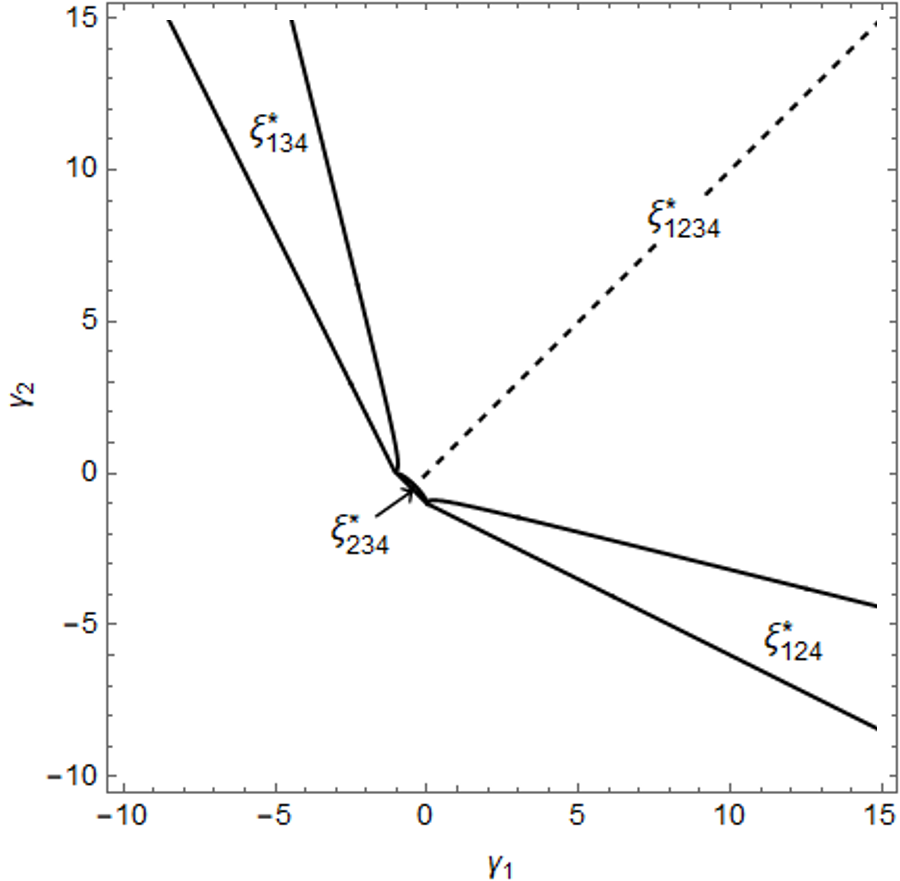
Refer to caption
(a)
Refer to caption
(b)
Figure 3: Dependence of locally D-optimal designs on γ1=β1/β3subscript𝛾1subscript𝛽1subscript𝛽3\gamma_{1}=\beta_{1}/\beta_{3} and γ2=β2/β3subscript𝛾2subscript𝛽2subscript𝛽3\gamma_{2}=\beta_{2}/\beta_{3} where for Panel (a) 𝒳=[1,2]2𝒳superscript122\mathcal{X}=[1,2]^{2} and for Panel (b) 𝒳=[1,4]2𝒳superscript142\mathcal{X}=[1,4]^{2}. The diagonal dashed line represents the case γ2=γ1subscript𝛾2subscript𝛾1\gamma_{2}=\gamma_{1}. Note that supp(ξijk)={𝒗i,𝒗j,𝒗k}{𝒗1,𝒗2,𝒗3,𝒗4}suppsubscriptsuperscript𝜉𝑖𝑗𝑘subscript𝒗𝑖subscript𝒗𝑗subscript𝒗𝑘subscript𝒗1subscript𝒗2subscript𝒗3subscript𝒗4\mathrm{supp}(\xi^{*}_{ijk})=\{\boldsymbol{v}_{i},\boldsymbol{v}_{j},\boldsymbol{v}_{k}\}\subset\{\boldsymbol{v}_{1},\boldsymbol{v}_{2},\boldsymbol{v}_{3},\boldsymbol{v}_{4}\} and supp(ξ1234)={𝒗1,𝒗2,𝒗3,𝒗4}suppsubscriptsuperscript𝜉1234subscript𝒗1subscript𝒗2subscript𝒗3subscript𝒗4\mathrm{supp}(\xi^{*}_{1234})=\{\boldsymbol{v}_{1},\boldsymbol{v}_{2},\boldsymbol{v}_{3},\boldsymbol{v}_{4}\}.

.

For arbitrary values of a𝑎a and b𝑏b, 0<a<b0𝑎𝑏0<a<b let us restrict to case γ2=γ1=γsubscript𝛾2subscript𝛾1𝛾\gamma_{2}=\gamma_{1}=\gamma, i.e., β1=β2=β,β30formulae-sequencesubscript𝛽1subscript𝛽2𝛽subscript𝛽30\beta_{1}=\beta_{2}=\beta,\beta_{3}\neq 0 and the next corollary is immediate.

Corollary 4.2.

Consider 𝐟(𝐱)=(x1,x2,x1x2)𝖳𝐟𝐱superscriptsubscript𝑥1subscript𝑥2subscript𝑥1subscript𝑥2𝖳\boldsymbol{f}(\boldsymbol{x})=(x_{1},x_{2},x_{1}x_{2})^{\sf T} on an arbitrary square 𝒳=[a,b]2, 0<a<bformulae-sequence𝒳superscript𝑎𝑏2 0𝑎𝑏\mathcal{X}=[a,b]^{2},\,0<a<b in the positive quadrant. Let β1=β2=βsubscript𝛽1subscript𝛽2𝛽\beta_{1}=\beta_{2}=\beta and β30subscript𝛽30\beta_{3}\neq 0. Define γ=ββ3𝛾𝛽subscript𝛽3\gamma=\frac{\beta}{\beta_{3}}. Then the locally D-optimal design ξsuperscript𝜉\xi^{*} (at 𝛃𝛃\boldsymbol{\beta}) is as follows.

  1. (i)

    If a2<γab3ba𝑎2𝛾𝑎𝑏3𝑏𝑎-\frac{a}{2}<\gamma\leq-\frac{ab}{3b-a}, then ξsuperscript𝜉\xi^{*} assigns equal weights 1/3131/3 to 𝒗2,𝒗3subscript𝒗2subscript𝒗3\boldsymbol{v}_{2},\boldsymbol{v}_{3}, 𝒗4subscript𝒗4\boldsymbol{v}_{4}.

  2. (ii)

    If b3a>0𝑏3𝑎0b-3a>0 and γabb3a𝛾𝑎𝑏𝑏3𝑎\gamma\geq\frac{ab}{b-3a}, then ξsuperscript𝜉\xi^{*} assigns equal weights 1/3131/3 to 𝒗1,𝒗2,𝒗3subscript𝒗1subscript𝒗2subscript𝒗3\boldsymbol{v}_{1},\boldsymbol{v}_{2},\boldsymbol{v}_{3}.

  3. (iii)

    If b3a>0𝑏3𝑎0b-3a>0 and ab3ba<γ<abb3a𝑎𝑏3𝑏𝑎𝛾𝑎𝑏𝑏3𝑎-\frac{ab}{3b-a}<\gamma<\frac{ab}{b-3a} then the design ξsuperscript𝜉\xi^{*} is supported by 𝒗1subscript𝒗1\boldsymbol{v}_{1}, 𝒗2,𝒗3subscript𝒗2subscript𝒗3\boldsymbol{v}_{2},\boldsymbol{v}_{3}, 𝒗4subscript𝒗4\boldsymbol{v}_{4}. The optimal weights are given by

    ω1=ab(a3b)γ4b(a+2γ),ω2=ω3=(ab+(a+b)γ)24ab(b+2γ)(a+2γ),ω4=ab(b3a)γ4a(b+2γ).formulae-sequenceformulae-sequencesuperscriptsubscript𝜔1𝑎𝑏𝑎3𝑏𝛾4𝑏𝑎2𝛾superscriptsubscript𝜔2superscriptsubscript𝜔3superscript𝑎𝑏𝑎𝑏𝛾24𝑎𝑏𝑏2𝛾𝑎2𝛾superscriptsubscript𝜔4𝑎𝑏𝑏3𝑎𝛾4𝑎𝑏2𝛾\omega_{1}^{*}=\frac{ab-(a-3b)\gamma}{4b(a+2\gamma)},\ \ \omega_{2}^{*}=\omega_{3}^{*}=\frac{\big{(}ab+(a+b)\gamma\big{)}^{2}}{4ab(b+2\gamma)(a+2\gamma)},\ \ \omega_{4}^{*}=\frac{ab-(b-3a)\gamma}{4a(b+2\gamma)}.
Proof.

Consider the experimental region 𝒳=[a,b]2, 0<a<bformulae-sequence𝒳superscript𝑎𝑏2 0𝑎𝑏\mathcal{X}=[a,b]^{2},\,0<a<b. By assumption β1=β2=β,β30formulae-sequencesubscript𝛽1subscript𝛽2𝛽subscript𝛽30\beta_{1}=\beta_{2}=\beta,\,\beta_{3}\neq 0 the range of γ=ββ3𝛾𝛽subscript𝛽3\gamma=\frac{\beta}{\beta_{3}} is given by (a/2,)𝑎2(-a/2,\infty). Assumption b3a>0𝑏3𝑎0b-3a>0 implies that a2<ab3ba<abb3a𝑎2𝑎𝑏3𝑏𝑎𝑎𝑏𝑏3𝑎-\frac{a}{2}<-\frac{ab}{3b-a}<\frac{ab}{b-3a}. Employing Corollary 4.1 shows the following. Both conditions of parts (ii𝑖𝑖ii) and (iii𝑖𝑖𝑖iii) of Corollary 4.1 are not fulfilled by any parameter point thus the corresponding designs are not D-optimal. In contrast, the design ξsuperscript𝜉\xi^{*} in (i𝑖i) of Corollary 4.2 is locally D-optimal if the condition of part (v)𝑣(v) of Corollary 4.1 holds true. That condition is equivalent to

(3b2+2aba2)γ2+4ab2γ+a2b20.3superscript𝑏22𝑎𝑏superscript𝑎2superscript𝛾24𝑎superscript𝑏2𝛾superscript𝑎2superscript𝑏20(3b^{2}+2ab-a^{2})\gamma^{2}+4ab^{2}\gamma+a^{2}b^{2}\leq 0.

The l.h.s. of above inequality is polynomial in γ𝛾\gamma of degree 2 and thus the inequality is fulfilled by a2<γab3ba𝑎2𝛾𝑎𝑏3𝑏𝑎-\frac{a}{2}<\gamma\leq-\frac{ab}{3b-a}.
Again, the design ξsuperscript𝜉\xi^{*} in (ii𝑖𝑖ii) is locally D-optimal if the condition of part (i)𝑖(i) of Corollary 4.1 holds true. That condition is equivalent to

(3a2+2abb2)γ2+4a2bγ+a2b20.3superscript𝑎22𝑎𝑏superscript𝑏2superscript𝛾24superscript𝑎2𝑏𝛾superscript𝑎2superscript𝑏20(3a^{2}+2ab-b^{2})\gamma^{2}+4a^{2}b\gamma+a^{2}b^{2}\leq 0.

The l.h.s. of above inequality is polynomial in γ𝛾\gamma of degree 2 and thus the inequality is fulfilled by γabb3a𝛾𝑎𝑏𝑏3𝑎\gamma\geq\frac{ab}{b-3a} if b3a>0𝑏3𝑎0b-3a>0.
The four-point design given in (iii𝑖𝑖𝑖iii) has positive weights on ab3ba<γ<abb3a𝑎𝑏3𝑏𝑎𝛾𝑎𝑏𝑏3𝑎-\frac{ab}{3b-a}<\gamma<\frac{ab}{b-3a} if b3a>0𝑏3𝑎0b-3a>0 and hence it is implicitly locally D-optimal by Remark 2. ∎

Remark 9.

One should note that from Corollary 4.2 when β=0𝛽0\beta=0 the uniform design on the vertices 𝐯1,𝐯2,𝐯3,𝐯4subscript𝐯1subscript𝐯2subscript𝐯3subscript𝐯4\boldsymbol{v}_{1},\boldsymbol{v}_{2},\boldsymbol{v}_{3},\boldsymbol{v}_{4} is locally D-optimal.

5 Design efficiency

The D-optimal design for gamma models depends on a given value of the parameter 𝜷𝜷\boldsymbol{\beta}. Misspecified values may lead to a poor performance of the locally optimal design. From our results the designs are locally D-optimal at a specific subregion of the parameter space. In this section we discuss the potential benefits of the derived designs, in particular, the D-optimal designs from Theorem 3.3 for a gamma model without interaction and from Corollary 4.2 for a gamma model with interaction. Our objective is to examine the overall performance of some of the locally D-optimal designs. The overall performance of any design ξ𝜉\xi is described by its D-efficiencies, as a function of 𝜷𝜷\boldsymbol{\beta},

Eff(ξ,𝜷)=(det𝑴(ξ,𝜷)det𝑴(ξ𝜷,𝜷))1/3Eff𝜉𝜷superscript𝑴𝜉𝜷𝑴superscriptsubscript𝜉𝜷𝜷13\displaystyle\mathrm{Eff}(\xi,\boldsymbol{\beta})=\left(\frac{\det\boldsymbol{M}(\xi,\boldsymbol{\beta})}{\det\boldsymbol{M}(\xi_{\boldsymbol{\beta}}^{*},\boldsymbol{\beta})}\right)^{1/3} (5.1)

where ξ𝜷superscriptsubscript𝜉𝜷\xi_{\boldsymbol{\beta}}^{*} denotes the locally D-optimal design at 𝜷𝜷\boldsymbol{\beta}.

Example 1. In the situation of Theorem 3.3 the experimental region is given by 𝒳=[1,2]3𝒳superscript123\mathcal{X}=[1,2]^{3}. We restrict only to the case β1>0subscript𝛽10\beta_{1}>0, β2=β3=βsubscript𝛽2subscript𝛽3𝛽\beta_{2}=\beta_{3}=\beta and hence we utilize the ratio γ=β/β1𝛾𝛽subscript𝛽1\gamma=\beta/\beta_{1} with range (1/4,)14(-1/4,\infty). Our interest is in the saturated and equally weighted designs ξ1subscript𝜉1\xi_{1} and ξ2subscript𝜉2\xi_{2} where supp(ξ1)={𝒗2,𝒗3,𝒗4}suppsubscript𝜉1subscript𝒗2subscript𝒗3subscript𝒗4\mathrm{supp}(\xi_{1})=\{\boldsymbol{v}_{2},\boldsymbol{v}_{3},\boldsymbol{v}_{4}\} and supp(ξ2)={𝒗3,𝒗4,𝒗5}suppsubscript𝜉2subscript𝒗3subscript𝒗4subscript𝒗5\mathrm{supp}(\xi_{2})=\{\boldsymbol{v}_{3},\boldsymbol{v}_{4},\boldsymbol{v}_{5}\} which by Theorem 3.3 are locally D-optimal at γ1/5𝛾15\gamma\geq 1/5 and γ(1/4,5/23]𝛾14523\gamma\in(-1/4,-5/23], respectively. In particular, ξ1subscript𝜉1\xi_{1} and ξ2subscript𝜉2\xi_{2} are robust against misspecified parameter values in their respective subregions. Additionally, for γ(5/23,1/5)𝛾52315\gamma\in(-5/23,1/5) we consider the locally D-optimal designs of type ξ3(γ)subscript𝜉3𝛾\xi_{3}(\gamma) given by the theorem. Note that supp(ξ3(γ))={𝒗2,𝒗3,𝒗4,𝒗5}suppsubscript𝜉3𝛾subscript𝒗2subscript𝒗3subscript𝒗4subscript𝒗5\mathrm{supp}(\xi_{3}(\gamma))=\{\boldsymbol{v}_{2},\boldsymbol{v}_{3},\boldsymbol{v}_{4},\boldsymbol{v}_{5}\} and the weights depend on γ𝛾\gamma.

To employ (5.1) we put ξ𝜷=ξ1superscriptsubscript𝜉𝜷subscript𝜉1\xi_{\boldsymbol{\beta}}^{*}=\xi_{1} if γ1/5𝛾15\gamma\geq 1/5, ξ𝜷=ξ2superscriptsubscript𝜉𝜷subscript𝜉2\xi_{\boldsymbol{\beta}}^{*}=\xi_{2} if γ(1/4,5/23]𝛾14523\gamma\in(-1/4,-5/23] and ξ𝜷=ξ3(γ)superscriptsubscript𝜉𝜷subscript𝜉3𝛾\xi_{\boldsymbol{\beta}}^{*}=\xi_{3}(\gamma) if γ(5/23,1/5)𝛾52315\gamma\in(-5/23,1/5). We select for examination the designs ξ1subscript𝜉1\xi_{1}, ξ2subscript𝜉2\xi_{2}, ξ3(1/7)subscript𝜉317\xi_{3}(-1/7). Moreover, as natural competitors we select various uniform designs supported by specific vertices. That is ξ4subscript𝜉4\xi_{4} with support {1,2}3superscript123\{1,2\}^{3} and the two half-fractional designs ξ5subscript𝜉5\xi_{5} and ξ6subscript𝜉6\xi_{6} supported by {𝒗1,𝒗5,𝒗6,𝒗7}subscript𝒗1subscript𝒗5subscript𝒗6subscript𝒗7\{\boldsymbol{v}_{1},\boldsymbol{v}_{5},\boldsymbol{v}_{6},\boldsymbol{v}_{7}\} and {𝒗2,𝒗3,𝒗4,𝒗8}subscript𝒗2subscript𝒗3subscript𝒗4subscript𝒗8\{\boldsymbol{v}_{2},\boldsymbol{v}_{3},\boldsymbol{v}_{4},\boldsymbol{v}_{8}\}, respectively. Additionally, we consider ξ7subscript𝜉7\xi_{7} which assigns uniform weights to the grid {1,1.5,2}3superscript11.523\{1,1.5,2\}^{3}.

In Panel (a) of Figure 4, the D-efficiencies of the designs ξ1subscript𝜉1\xi_{1}, ξ2subscript𝜉2\xi_{2}, ξ3(1/7)subscript𝜉317\xi_{3}(-1/7), ξ4subscript𝜉4\xi_{4}, ξ5subscript𝜉5\xi_{5}, ξ6subscript𝜉6\xi_{6} and ξ7subscript𝜉7\xi_{7} are depicted. The efficiencies of ξ1subscript𝜉1\xi_{1} and ξ2subscript𝜉2\xi_{2} are, of course, equal to 111 in their optimality subregions γ[1/5,)𝛾15\gamma\in[1/5,\infty) and γ(1/4,5/23]𝛾14523\gamma\in(-1/4,-5/23], respectively. However, for γ𝛾\gamma outside but fairly close to the respective optimality subregion both designs perform quite well; the efficiencies of ξ1subscript𝜉1\xi_{1} and ξ2subscript𝜉2\xi_{2} are greater than 0.800.800.80 for 0.15γ<1/50.15𝛾15-0.15\leq\gamma<1/5 and 1/4<γ0.2814𝛾0.28-1/4<\gamma\leq-0.28, respectively. However, their efficiencies decrease towards zero when γ𝛾\gamma moves away from the respective optimality subregion. So, the overall performance of ξ1subscript𝜉1\xi_{1} and ξ2subscript𝜉2\xi_{2} cannot be regarded as satisfactory. The design ξ3(1/7)subscript𝜉317\xi_{3}(-1/7), though locally D-optimal only at γ=1/7𝛾17\gamma=-1/7, does show a more satisfactory overall performance with efficiencies range between 0.85850.85850.8585 and 111. The efficiencies of the half-fractional design ξ6subscript𝜉6\xi_{6} are greater than 0.800.800.80 only for γ>0.049𝛾0.049\gamma>-0.049, otherwise the efficiencies decrease towards zero. The design ξ4subscript𝜉4\xi_{4} turns out to be uniformly worse than ξ3(1/7)subscript𝜉317\xi_{3}(-1/7) and its efficiencies range between 0.57680.57680.5768 and 0.76150.76150.7615. The worst performance is shown by the designs ξ5subscript𝜉5\xi_{5} and ξ7subscript𝜉7\xi_{7}.

Example 2. In the situation of Corollary 4.2 we consider the experimental region 𝒳=[1,4]2𝒳superscript142\mathcal{X}=[1,4]^{2} where condition b3a>0𝑏3𝑎0b-3a>0 is satisfied. The vertices are denoted by 𝒗1=(4,4)𝖳subscript𝒗1superscript44𝖳\boldsymbol{v}_{1}=\big{(}4,4\big{)}^{\sf T}, 𝒗2=(4,1)𝖳subscript𝒗2superscript41𝖳\boldsymbol{v}_{2}=\big{(}4,1\big{)}^{\sf T}, 𝒗3=(1,4)𝖳subscript𝒗3superscript14𝖳\boldsymbol{v}_{3}=\big{(}1,4\big{)}^{\sf T}, 𝒗4=(1,1)𝖳subscript𝒗4superscript11𝖳\boldsymbol{v}_{4}=\big{(}1,1\big{)}^{\sf T}. We restrict to β30subscript𝛽30\beta_{3}\neq 0, β1=β2=βsubscript𝛽1subscript𝛽2𝛽\beta_{1}=\beta_{2}=\beta, and the range of γ=β/β3𝛾𝛽subscript𝛽3\gamma=\beta/\beta_{3} is (1/2,)12(-1/2,\infty). In analogy to Example 1 denote by ξ1subscript𝜉1\xi_{1} and ξ2subscript𝜉2\xi_{2} the saturated and equally weighted designs with support {𝒗1,𝒗2,𝒗3}subscript𝒗1subscript𝒗2subscript𝒗3\{\boldsymbol{v}_{1},\boldsymbol{v}_{2},\boldsymbol{v}_{3}\} and {𝒗2,𝒗3,𝒗4}subscript𝒗2subscript𝒗3subscript𝒗4\{\boldsymbol{v}_{2},\boldsymbol{v}_{3},\boldsymbol{v}_{4}\}, respectively. By the corollary ξ1subscript𝜉1\xi_{1} and ξ2subscript𝜉2\xi_{2} are locally D-optimal at γ4𝛾4\gamma\geq 4 and γ(1/2,4/11]𝛾12411\gamma\in(-1/2,-4/11], restrictively. Denote by ξ3(γ)subscript𝜉3𝛾\xi_{3}(\gamma) the design given in part (ii)𝑖𝑖(ii) of Corollary 4.2 which is locally D-optimal at γ(4/11,4)𝛾4114\gamma\in(-4/11,4). Note that from (5.1) we put ξ𝜷=ξ1superscriptsubscript𝜉𝜷subscript𝜉1\xi_{\boldsymbol{\beta}}^{*}=\xi_{1} if γ4𝛾4\gamma\geq 4, ξ𝜷=ξ2superscriptsubscript𝜉𝜷subscript𝜉2\xi_{\boldsymbol{\beta}}^{*}=\xi_{2} if γ(1/2,4/11]𝛾12411\gamma\in(-1/2,-4/11] and ξ𝜷=ξ3(γ)superscriptsubscript𝜉𝜷subscript𝜉3𝛾\xi_{\boldsymbol{\beta}}^{*}=\xi_{3}(\gamma) if γ(4/11,4)𝛾4114\gamma\in(-4/11,4). For examination we select ξ1subscript𝜉1\xi_{1}, ξ2subscript𝜉2\xi_{2}, ξ3(0)subscript𝜉30\xi_{3}(0). As a natural competitor we select ξ4subscript𝜉4\xi_{4} that assigns uniform weights to the grid {1,2.5,4}2superscript12.542\{1,2.5,4\}^{2}. The efficiencies are depicted in Panel (b) of Figure 4. We observe that the performance of ξ1subscript𝜉1\xi_{1} and ξ2subscript𝜉2\xi_{2} is similar to that of the corresponding designs in Example 1. Moreover, the design ξ(0)𝜉0\xi(0) show a more satisfactory overall performance. The efficiencies of ξ4subscript𝜉4\xi_{4} vary between 0.770.770.77 and 0.830.830.83 for γ>4/11𝛾411\gamma>-4/11.

Refer to caption
(a) Example 1. The considered interval is 1/4<γ114𝛾1-1/4<\gamma\leq 1.
Refer to caption
(b) Example 2. The considered interval is 1/2<γ512𝛾5-1/2<\gamma\leq 5.
Figure 4: D-efficiencies from (5.1) of particular designs relative to the optimal designs at their optimality subregions under gamma models without intercept.

6 Conclusion

In the current paper we considered gamma models without intercept for which locally D- and A-optimal designs have been developed. The positivity of the expected means entails a positive linear predictor whereas absence of the intercept term requires an experimental region which is not containing the origin point 𝟎0\boldsymbol{0}. The information matrix for the non-intercept gamma model is invariant w.r.t. simultaneously scaling of 𝒙𝒙\boldsymbol{x} or 𝜷𝜷\boldsymbol{\beta}. In this context, we utilized different approaches to derive the locally optimal designs. Sets of D- and A-optimal designs were derived on a non-compact experimental region. On the other hand, a transformation to models that are having intercept were employed on a two-factor model without or with interaction as in Theorem 3.2 or Corollary 4.1, respectively. This approach simplified the optimality problem and thus such known results were applied. Moreover, the complexity of applying The Equivalence Theorem as in Theorem 3.3 implicated the optimality problem to solve a system of inequalities analytically or by employing computer algebra. In contrast, the transformation approach, of course, can be used for the case in Theorem 3.3 and thus according to Remark 6, the three-factor model without intercept on 𝒳=[1,2]2𝒳superscript122\mathcal{X}=[1,2]^{2} can be transformed to a model with intercept on  𝒯=Conv{(1/2,1)𝖳,(1,1/2)𝖳,(1/2,1/2)𝖳,(2,1)𝖳,(1,2)𝖳,(2,2)𝖳}𝒯Convsuperscript121𝖳superscript112𝖳superscript1212𝖳superscript21𝖳superscript12𝖳superscript22𝖳\mathcal{T}={\rm Conv}\bigl{\{}(1/2,1)^{\sf T},(1,1/2)^{\sf T},(1/2,1/2)^{\sf T},(2,1)^{\sf T},(1,2)^{\sf T},(2,2)^{\sf T}\bigr{\}}. Rescaling 𝒯𝒯\mathcal{T} yields 𝒵=Conv{(0,1/3)𝖳,(1/3,0)𝖳,(0,0)𝖳,(1,1/3)𝖳,(1/3,1)𝖳,(1,1)𝖳}𝒵Convsuperscript013𝖳superscript130𝖳superscript00𝖳superscript113𝖳superscript131𝖳superscript11𝖳\mathcal{Z}={\rm Conv}\bigl{\{}(0,1/3)^{\sf T},(1/3,0)^{\sf T},(0,0)^{\sf T},(1,1/3)^{\sf T},(1/3,1)^{\sf T},(1,1)^{\sf T}\bigr{\}}. Consequently, the linear predictor is reparameterized as β~0+β~1z1+β~2z2subscript~𝛽0subscript~𝛽1subscript𝑧1subscript~𝛽2subscript𝑧2\tilde{\beta}_{0}+\tilde{\beta}_{1}z_{1}+\tilde{\beta}_{2}z_{2} where (z1,z2)𝖳𝒵superscriptsubscript𝑧1subscript𝑧2𝖳𝒵(z_{1},z_{2})^{\sf T}\in{\mathcal{Z}} and β~0=β1+(1/2)(β2+β3)subscript~𝛽0subscript𝛽112subscript𝛽2subscript𝛽3\tilde{\beta}_{0}=\beta_{1}+(1/2)(\beta_{2}+\beta_{3}), β~1=(3/2)β2subscript~𝛽132subscript𝛽2\tilde{\beta}_{1}=(3/2)\beta_{2}, β~2=(3/2)β3subscript~𝛽232subscript𝛽3\tilde{\beta}_{2}=(3/2)\beta_{3}.

In many applied aspects, the log-link function is considered as a main alternative to the canonical one (see Kilian et al. (2002),Wenig et al. (2009),Gregori et al. (2011),McCrone et al. (2005),Montez-Rath et al. (2006)). In that case the intensity function u(𝒙,𝜷)=1𝑢𝒙𝜷1u(\boldsymbol{x},\boldsymbol{\beta})=1 and thus the information matrix under gamma models is equivalent to that under ordinary regression models. For that reason, the optimal designs for a gamma model are identical to those for an ordinary regression model with similar linear predictor. In Hardin and Hilbe (2018) gamma models were fitted considering various link functions, for example; the Box-Cox family of link functions that is given by

𝒇𝖳(𝒙)𝜷={(μλ1)/λ(λ0)logμ(λ=0)superscript𝒇𝖳𝒙𝜷casessuperscript𝜇𝜆1𝜆𝜆0𝜇𝜆0\boldsymbol{f}^{\sf T}(\boldsymbol{x})\boldsymbol{\beta}=\left\{\begin{array}[]{ll}\bigl{(}\mu^{\lambda}-1\bigr{)}/\lambda&(\lambda\neq 0)\\ \log\mu&(\lambda=0)\end{array}\right. (6.1)

which involves the log-link at λ=0𝜆0\lambda=0 (see Atkinson and Woods (2015)). The intensity function is thus defined as

u(𝒙,λ𝜷)=(λ𝒇𝖳(𝒙)𝜷+1)2,𝒙𝒳.formulae-sequence𝑢𝒙𝜆𝜷superscript𝜆superscript𝒇𝖳𝒙𝜷12𝒙𝒳u(\boldsymbol{x},\lambda\boldsymbol{\beta})=\big{(}\lambda\boldsymbol{f}^{\sf T}(\boldsymbol{x})\boldsymbol{\beta}+1\big{)}^{-2},\boldsymbol{x}\in\mathcal{X}. (6.2)

Here, the positivity condition (2.5) of the expected mean μ=E(y)𝜇𝐸𝑦\mu=E(y) of a gamma distribution is modified to λ𝒇𝖳(𝒙)𝜷>1𝜆superscript𝒇𝖳𝒙𝜷1\lambda\boldsymbol{f}^{\sf T}(\boldsymbol{x})\boldsymbol{\beta}>-1 for all 𝒙𝒳𝒙𝒳\boldsymbol{x}\in\mathcal{X}. Therefore, for a gamma model without intercept the experimental region might be considered as 𝒳=[0,1]ν𝒳superscript01𝜈\mathcal{X}=[0,1]^{\nu}. As an example, consider 𝒇(𝒙)=(x1,x2)𝖳𝒇𝒙superscriptsubscript𝑥1subscript𝑥2𝖳\boldsymbol{f}(\boldsymbol{x})=(x_{1},x_{2})^{\sf T} on 𝒳=[0,1]2𝒳superscript012\mathcal{X}=[0,1]^{2} with vertices 𝒗1=(0,0)𝖳subscript𝒗1superscript00𝖳\boldsymbol{v}_{1}=(0,0)^{\sf T}, 𝒗2=(1,0)𝖳subscript𝒗2superscript10𝖳\boldsymbol{v}_{2}=(1,0)^{\sf T}, 𝒗3=(0,1)𝖳subscript𝒗3superscript01𝖳\boldsymbol{v}_{3}=(0,1)^{\sf T}, 𝒗4=(1,1)𝖳subscript𝒗4superscript11𝖳\boldsymbol{v}_{4}=(1,1)^{\sf T}. Let uk=u(𝒗k,λ𝜷)subscript𝑢𝑘𝑢subscript𝒗𝑘𝜆𝜷u_{k}=u(\boldsymbol{v}_{k},\lambda\boldsymbol{\beta}) for all (1k4)1𝑘4(1\leq k\leq 4). The Equivalence Theorem (Theorem 2.1, part (a)) approves the D-optimality of the design ξsuperscript𝜉\xi^{*} which assigns equal weights 1/2121/2 to the vertices 𝒗2subscript𝒗2\boldsymbol{v}_{2} and 𝒗3subscript𝒗3\boldsymbol{v}_{3} at the point λ𝜷𝜆𝜷\lambda\boldsymbol{\beta}. This result might be extended for a multiple-factor model as in Theorem 3.1. However, the expression λ𝒇𝖳(𝒙)𝜷+1𝜆superscript𝒇𝖳𝒙𝜷1\lambda\boldsymbol{f}^{\sf T}(\boldsymbol{x})\boldsymbol{\beta}+1 could be viewed as a linear predictor of a gamma model with known intercept. Adopting the Box-Cox family as a class of link functions for gamma models could be a topic of future research.

References

  • Atkinson and Woods (2015) Atkinson, A.C., Woods, D.C., 2015. Designs for generalized linear models. Handbook of Design and Analysis of Experiments , 471–514.
  • Burridge and Sebastiani (1992) Burridge, J., Sebastiani, P., 1992. Optimal designs for generalized linear models. Journal of the Italian Statistical Society 1, 183–202. URL: https://doi.org/10.1007/BF02589030.
  • Burridge and Sebastiani (1994) Burridge, J., Sebastiani, P., 1994. D-optimal designs for generalised linear models with variance proportional to the square of the mean. Biometrika 81, 295–304. URL: http://www.jstor.org/stable/2336960.
  • Chatterjee (1988) Chatterjee, S., 1988. Sensitivity Analysis in Linear Regression. John Wiley & Sons, Inc., New York, NY, USA.
  • Ford et al. (1992) Ford, I., Torsney, B., Wu, C.F.J., 1992. The use of a canonical form in the construction of locally optimal designs for non-linear problems. Journal of the Royal Statistical Society. Series B (Methodological) 54, 569–583. URL: http://www.jstor.org/stable/2346142.
  • Gaffke et al. (2018) Gaffke, N., Idais, O., Schwabe, R., 2018. Locally optimal designs for gamma models. Manuscript under revision .
  • Gea-Izquierdo and Cañellas (2009) Gea-Izquierdo, G., Cañellas, I., 2009. Analysis of Holm Oak Intraspecific Competition Using Gamma Regression. Forest Science 55, 310–322. URL: https://dx.doi.org/10.1093/forestscience/55.4.310.
  • Gregori et al. (2011) Gregori, D., Pagano, E., Merletti, F., Petrinco, M., Bo, S., Desideri, A., 2011. Regression models for analyzing costs and their determinants in health care: an introductory review. International Journal for Quality in Health Care 23, 331–341. URL: https://dx.doi.org/10.1093/intqhc/mzr010.
  • Grover et al. (2013) Grover, G., Sabharwal, A.K., Mittal, J., 2013. An Application of Gamma Generalized Linear Model for Estimation of Survival Function of Diabetic Nephropathy Patients. International Journal of Statistics in Medical Research 2, 209–219.
  • Hardin and Hilbe (2018) Hardin, J.W., Hilbe, J.M., 2018. Generalized linear models and extensions. Stata Press.
  • Harman and Trnovská (2009) Harman, R., Trnovská, M., 2009. Approximate d-optimal designs of experiments on the convex hull of a finite set of information matrices. Mathematica Slovaca 59, 693. URL: https://doi.org/10.2478/s12175-009-0157-9.
  • Kiefer and Wolfowitz (1960) Kiefer, J., Wolfowitz, J., 1960. The equivalence of two extremum problems. Canadian Journal of Mathematics 12, 363–366. doi:10.4153/CJM-1960-030-4.
  • Kilian et al. (2002) Kilian, R., Matschinger, H., Löeffler, W., Roick, C., Angermeyer, M.C., 2002. A comparison of methods to handle skew distributed cost variables in the analysis of the resource consumption in schizophrenia treatment. The journal of mental health policy and economics 5 1, 21–31.
  • Kurtoğlu and Özkale (2016) Kurtoğlu, F., Özkale, M.R., 2016. Liu estimation in generalized linear models: application on gamma distributed response variable. Statistical Papers 57, 911–928. URL: https://doi.org/10.1007/s00362-016-0814-3.
  • McCrone et al. (2005) McCrone, P., Knapp, M., Fombonne, E., 2005. The maudsley long-term follow-up of child and adolescent depression. European Child & Adolescent Psychiatry 14, 407–413. doi:10.1007/s00787-005-0491-6.
  • McCullagh and Nelder (1989) McCullagh, P., Nelder, J., 1989. Generalized Linear Models, Second Edition. Chapman and Hall/CRC Monographs on Statistics and Applied Probability Series, Chapman & Hall. URL: http://books.google.com/books?id=h9kFH2_FfBkC.
  • Montez-Rath et al. (2006) Montez-Rath, M., Christiansen, C.L., Ettner, S.L., Loveland, S., Rosen, A.K., 2006. Performance of statistical models to predict mental health and substance abuse cost. BMC Medical Research Methodology 6, 53. doi:10.1186/1471-2288-6-53.
  • Ng and Cribbie (2017) Ng, V.K., Cribbie, R.A., 2017. Using the gamma generalized linear model for modeling continuous, skewed and heteroscedastic outcomes in psychology. Current Psychology 36, 225–235. URL: https://doi.org/10.1007/s12144-015-9404-0.
  • R Core Team (2018) R Core Team, 2018. R: A Language and Environment for Statistical Computing. R Foundation for Statistical Computing. Vienna, Austria. URL: https://www.R-project.org.
  • Radloff and Schwabe (2016) Radloff, M., Schwabe, R., 2016. Invariance and equivariance in experimental design for nonlinear models, in: mODa 11-Advances in Model-Oriented Design and Analysis. Springer, pp. 217–224.
  • Silvey (1980) Silvey, S., 1980. Optimal design: an introduction to the theory for parameter estimation. Monographs on applied probability and statistics, Chapman and Hall. URL: https://books.google.de/books?id=uXGmAAAAIAAJ.
  • Wenig et al. (2009) Wenig, C.M., Schmidt, C.O., Kohlmann, T., Schweikert, B., 2009. Costs of back pain in germany. European Journal of Pain 13, 280–286.
  • (23) Wolfram Research, I., . Mathematica, Version 11.3. Champaign, IL, 2018.
  • Yu (2010) Yu, Y., 2010. Monotonic convergence of a general algorithm for computing optimal designs. The Annals of Statistics , 1593–1606.