Polarimetric Thermal to Visible Face Verification
via Self-Attention Guided Synthesis
Abstract
Polarimetric thermal to visible face verification entails matching two images that contain significant domain differences. Several recent approaches have attempted to synthesize visible faces from thermal images for cross-modal matching. In this paper, we take a different approach in which rather than focusing only on synthesizing visible faces from thermal faces, we also propose to synthesize thermal faces from visible faces. Our intuition is based on the fact that thermal images also contain some discriminative information about the person for verification. Deep features from a pre-trained Convolutional Neural Network (CNN) are extracted from the original as well as the synthesized images. These features are then fused to generate a template which is then used for verification. The proposed synthesis network is based on the self-attention generative adversarial network (SAGAN) which essentially allows efficient attention-guided image synthesis. Extensive experiments on the ARL polarimetric thermal face dataset demonstrate that the proposed method achieves state-of-the-art performance.
1 Introduction
Recognizing faces in low-light/night-time with that in normal (visible) conditions is a very difficult problem. Besides the challenges including expression, pose variance, etc., significant distribution change in different spectrum domain also causes the huge difficulty. Various thermal imaging modalities have been introduced in the literature to deal with this problem. The infrared spectrum can be divided into a reflection dominated region consisting of the near infrared (NIR) and shortwave infrared (SWIR) bands, and an emission dominated thermal region consisting of the midwave infrared (MWIR) and longwave infrared (LWIR) bands [25]. It has been shown that polarimetric thermal imaging captures additional geometric and textural facial details compared to conventional thermal imaging [10]. Hence, the polarization-state information has been used to improve the performance of cross-spectrum face recognition [10, 27, 30, 35, 26, 5].
A polarimetric, referred to as Stokes images, is composed of three channels: S0, S1 and S2. Here, S0 represents the conventional intensity only thermal image, whereas S1 and S2 represent the horizontal/vertical and diagonal polarization-state information, respectively. In polarimetric thermal to visible face verification, given a pair of visible and polarimetric thermal images, the goal is to determine whether these images correspond to the same person. The large domain discrepancy between these images makes the cross-spectrum matching problem very challenging. Various methods have been proposed in the literature for cross-spectrum matching [10, 27, 30, 35, 26, 16, 21, 18, 2, 28, 24]. These approaches either attempt to synthesize visible faces from thermal faces or extract robust features from these modalities for cross-modal matching.
Hu et al. [9] proposed a partial least squares regression (PLS) method for this cross-modal matching. Klare et al. [17] developed a generic framework based on the kernel prototype nonlinear similarity for cross-modal matching. In [14] PLS-based discriminant analysis approaches were used to correlate the thermal face signatures to the visible face signatures. In addition, Riggan et al. [25] proposed a combination of PLS classifier with two different feature mapping approaches: Coupled Neural Network CpNN and Deep Perceptual Mapping (DPM) to utilize the features derived from the Stokes images for cross-modal face recognition. Recently, Iranmanesh et al. [11] proposed a two stream Deep Convolutional Neural Networks (DCNNs) (Vis-DCNN and Pol-DCNN) to learn a discriminative metric for this cross-domain verification. Some of the other visible to thermal cross-modal matching methods include [7, 29].
Various synthesis-based methods have also been proposed in the literature [26, 35, 38, 27] to perform cross-modal mapping at the image level for direct use in existing visible-based matchers. Riggan et al. [27] trained a regression network to estimate the mapping between features from both visible and thermal then reconstruct the visible face based on the estimated features. Zhang et al. [35, 36] leveraged generative adversarial networks (GANs) to synthesize visible images from polarimetric thermal images. Riggan et al. [26] proposed a global and local region-based synthesis network to transform the thermal image into the visible spectrum. In a recent work [5] Di et al. developed an attribute preserved adversarial network called AP-GAN to enhance the quality of the synthesized images. Zhang et al. [36] introduced a multi-stream dense-residual encoder-decoder network, which implemented a feature-level fusion techniques to solve the problem.
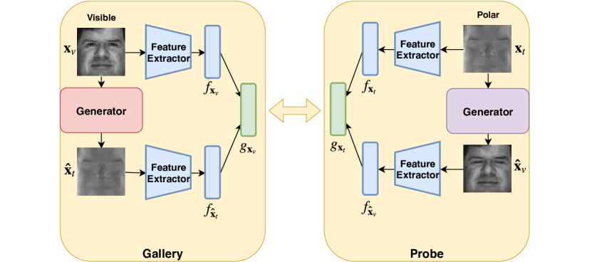
In this paper, we take a different approach to the problem of thermal to visible matching by exploring the complementary information of different modalities. Figure 1 gives an overview of the proposed approach. Given a thermal-visible pair (), these images are first transformed into their spectrum counterparts using two trained generators as , . Then a feature extractor network , in particular the VGG-Face model [23], is used to extract features , , , and . These features are then fused to generate the gallery template and the probe template . Finally, the cosine similarity score between these feature templates is calculated for verification.

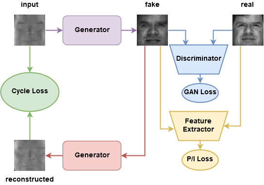
Note that CycleGAN-based networks [39] can be used to train these generators. However, experiments have shown that CycleGAN often fails to capture the geometric or struc- tural patterns around the eye and mouth regions. One possible reason could be that the network relies heavily on convolutions to model the dependencies across different image regions. The long range dependencies are not well captured by the local receptive field of convolutional layers [34]. For improvement, we adopt the self-attention techniques [3, 22, 31] from SAGAN [34]. The self-attention module is applied right before the last convolutional layer of the generator and the discriminator. Given the feature maps, this module learns the attention maps by itself with a softmax function and then the learned attention maps are multiplied with the feature maps to output the self-attention guided feature maps. In addition, the generator is optimized by an objective function consisting of the adversarial loss [6], loss, perceptual loss [13], identity loss [35] and cycle-consistency loss [39]. The entire synthesis framework is shown in Figure 2.
To summarize, the following are our main contributions:
-
•
A novel cross-spectral face verification framework is proposed in which a self-attention guided GAN is developed for synthesizing visible faces from the thermal and thermal faces from the visible.
- •
-
•
Extensive experiments are conducted on the ARL Facial Database [10] and comparisons are performed against several recent state-of-the-art approaches. Furthermore, an ablation study is conducted to demonstrate the effectiveness of the fusion approach proposed in this paper.
2 Proposed Method
In this section, we discuss details of the proposed self-attention guided synthesis method. In particular, we discuss the proposed generator and the discriminator networks as well as the loss functions used to train the network. The overall framework is shown in Figure 2. Given an input image from one modality (thermal as shown), it is first synthesized into the other modality (i.e. visible) using the proposed self-attention module-based generator. Then another generator with similar architecture is used to synthesize it back from the visible domain to the original thermal domain. In order to achieve the reconstruction back to original modality, these generators are trained using the cycle-consistency loss [39, 33]. In order to minimize the domain gap between the fake (i.e. synthesized) and real images, a patch-based pixel GAN loss is also introduced [12]. Furthermore, the semantic and identity information are captured by minimizing the perceptual and identity loss [4], respectively.
2.1 Generator
An encoder-decoder type of generator which is inspired by the residual network (He et al. [8]) and SAGAN (Han et al. [34]) is adopted in this work. In order to prevent the vanishing gradient problem, the residual block is implemented after a sequence of convolutional layers. For each residual block shown in Figure 3, it consists of two convolutional layers followed by batch-normalization and relu layers. In order to involve the facial long-range dependency information, we adopt the self-attention module into the generator. Self-attention module was proposed by Han et al. in SAGAN [34] which allows attention-driven, long-range dependency modeling for general image generation tasks. In our work, the self-attention module is inserted right before the last convolutional layer of the generator. The self-attention module, shown as in Figure 3, consists of two components: feature maps and attention maps. The feature maps are generated by a convolutional layer working on the input features. The attention maps are generated by the elementwise multiplication of two convolutional features followed by the softmax function. Finally, this module outputs the elementwise multiplication of feature maps and attention maps.
The self-attention module-based generator architecture is shown in Figure 3. This generator architecture is consists of the following components:
CBR(64)-CBR(128)-CBR(256)-Res(256)-Res(256)-Res(256)-Res(256)-Res(256)-DBL(128)-DBL(64)-SA(64)-CT(3),
where C stands for the convolutional layer (stride 2, kernel-size 4, and padding size 1). B and R stand for batch-normalization layer and relu layer, respectively. Res is the residual block [8], D denotes the deconvolutional layer (stride 2, kernel-size 4 and padding size 1), L is the leaky relu layer, SA is the self-attention module, and T is the tanh function layer. The numbers inside the parenthesis denote the number of channels corresponding to the output feature maps.
2.2 Discriminator
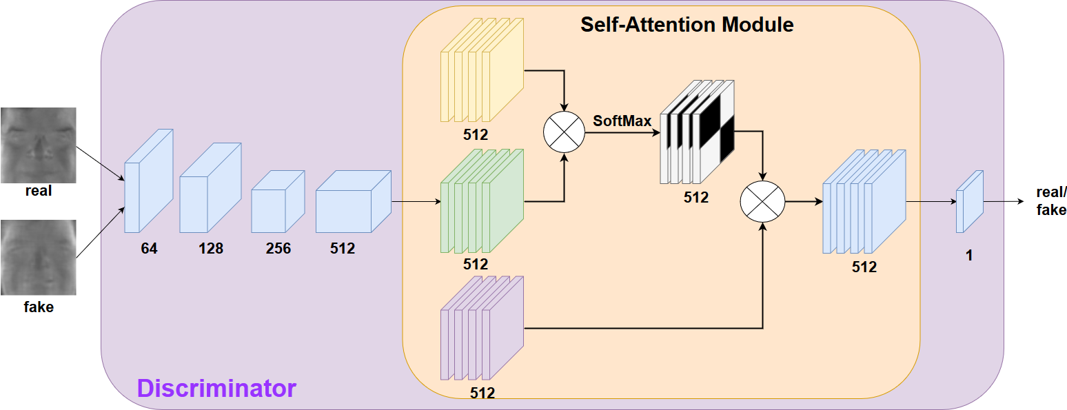
Motivated by pixel GAN [12], a patch-based discriminator is leveraged in the proposed method and is trained iteratively with the generator. In addition, in order to improve the stability of training, we adopt the spectral normalization to the discriminator [20]. Compared to the other normalization techniques, spectral normalization does not require extra hyper-parameter tuning and has a relatively small the computational cost. Similarly, in order to capture the long-range dependency information, a self-attention module is added before the last convolutional layer in the discriminator. The discriminator, as shown in Figure 4, consists of the following components:
CLSn(64)-CLSn(128)-CLSn(256)-CLSn(512)-CLS(n512)-SA(512)-CS(1),
where Sn stands for the spectral normalization layer. C, L, SA, S stand for the convolutional layer, leaky relu layer, self-attention module and sigmoid function, respectively. The numbers inside the parenthesis denote the number of channels corresponding to the output feature maps.
(a)
(b)

2.3 Objective Function
Given a set of thermal images and another set of visible images , the generator and discriminator networks are optimized iteratively by minimizing the following loss functions
where are the adversarial losses for two generators - one for synthesizing visible from thermal () and the other for synthesizing thermal from visible (). Similarly, is the perceptual loss, is the identity loss, is the loss based on the L1-norm between the target and the synthesized image, and are the weights for perceptual loss, identity loss and L1 loss, respectively.
2.3.1 Adversarial Loss
Similar to the Cycle-GAN work [39], there are two kinds adversarial losses. One for synthesizing visible image from thermal image and the other for synthesizing thermal image from visible image. Both are defined as follows:
| (1) |
where and are discriminators for visible and thermal modality, respectively. In addition, and are two generators for synthesizing thermal image from visible and synthesizing visible image from thermal, respectively.
2.3.2 Cycle-Consistency Loss
A cycle-consistency constraint is also imposed in our approach [39, 33] (see Figure 2 green portion). Taking thermal to visible synthesis as an example, we introduce one mapping from thermal to visible and train it according to the same GAN loss . We then require another mapping from thermal to visible and back to thermal which reproduces the original sample, thereby enforcing cycle-consistency. In other words, we want and . This is done by imposing an penalty on the reconstruction error, which is referred to as the cycle-consistency loss. It is defined as follows:
| (2) |
2.3.3 Perceptual, Identity and L1 Loss Functions
These loss functions can be implemented when we have supervised pairwise data , where and , during training. The L1 loss is defined as below:
| (3) |
In order to minimize the perceptual and identity information [13, 4], we implement the perceptual and identity loss functions as follows
where and are two off-the-shelf pretrained networks for extracting features. Since deeper features in hierarchical deep networks capture more semantic information, the output features and from the VGGFace pretrained network are used in the perceptual and the identity losses, respectively.
Note that if we omit the perceptual, identity and L1 loss functions which require pairwise supervised data, then one can also implement the proposed framework in completely unsupervised fashion. In other words, the proposed framework is also applicable to the case where the paired data are not available during training.
| Method | AUC (Polar) | AUC(S0) | EER(Polar) | EER(S0) |
| Raw | 50.35% | 58.64% | 48.96% | 43.96% |
| Mahendran et al. [19] | 58.38% | 59.25% | 44.56% | 43.56% |
| Riggan et al. [27] | 75.83% | 68.52% | 33.20% | 34.36% |
| GAN-VFS [35] | 79.90% | 79.30% | 25.17% | 27.34% |
| Riggan et al. [26] | 85.42% | 82.49% | 21.46% | 26.25% |
| AP-GAN [5] | ||||
| Multi-stream GAN [36] | % | 85.74% | % | 23.18% |
| Ours |
| Method | AUC (Polar) | AUC(S0) | EER(Polar) | EER(S0) |
| Raw | 66.85% | 63.66% | 37.85% | 40.93% |
| CycleGAN [39](unsupervised) | ||||
| ours(unsupervised †† , Identity and Perceptual losses are removed for training on unsupervised setting) | ||||
| Pix2Pix [12] | ||||
| Pix2PixBEGAN [12, 1] | ||||
| CycleGAN [39] (supervised) | ||||
| Multi-stream GAN [36] | % | – | % | – |
| Ours |
3 Experimental Results
The proposed method is evaluated on the ARL Multimodal Face Database [10] which consists of polarimetric (i.e. Stokes image) and visible images from Volume I [10] and II [36]. The Volume I data consists of images corresponding to 60 subjects. On the other hand, the Volume II data consists of images from 51 subjects (81 subjects in total). Similar to [27, 35, 36], we evaluate the proposed method based on two protocols. For Protocol I, images corresponding to Range 1 from 30 subjects are used for training. The remaining 30 subjects’ data are used for evaluation. For Protocol II, all images from 81 subjects are used for running experiments. Specifically, all images from Volume I and 25 subjects’ images from Volume II are used for training, the remaining 26 subjects’ images from Volume II are used for evaluation. We repeat this process 5 times and report the average results.
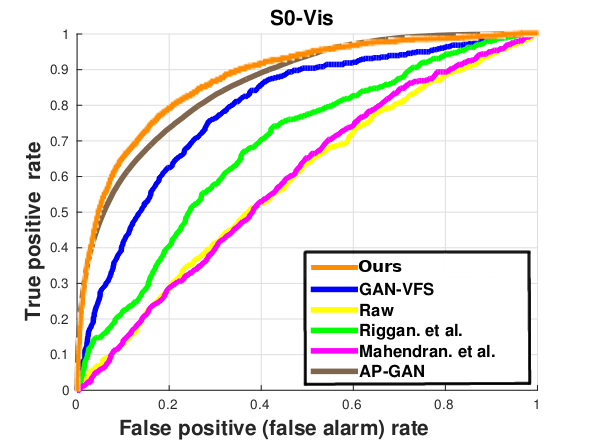
We evaluate the face verification performance of proposed method and compare it with several recent works [35, 26, 12, 39, 36]. Moreover, the performance is evaluated based on the FC-7 layer of the pretrained VGG-Face model [23] using the receiver operating characteristic (ROC) curve, Area Under the Curve (AUC) and Equal Error Rate (EER) measures. To summarize, the proposed method is evaluated on the following four experiments:
a) Conventional thermal (S0) to Visible (Vis) on Protocol I.
b) Polarimetric thermal (Polar) to Visible (Vis) on Protocol I.
c) Conventional thermal (S0) to Visible (Vis) on Protocol II.
d) Polarimetric thermal (Polar) to Visible (Vis) on Protocol II.
3.1 Implementation
In addition to the standard preprocessing as discussed in [10], two more preprocessing steps are used in the proposed method. First, the faces in the visible domain are detected by MTCNN [37]. Then, a standard central crop method is used to crop the registered faces. Since the MTCNN is implementable on the visible images only, we use the same detected rectangle coordination to crop the S0, S1, S2 images. After preprocessing, all the images are scaled to be and are saved as 16-bit PNG files.
The entire network is trained in Pytorch on a single Nvidia Titan-X GPU. The L1, perceptual and identity loss parameters are chosen as =10, = 2, = 0.2 respectively by a grid search. The ADAM [15] is implemented as the optimization algorithm with parameter betas = (0.5,0.999) and batch size is chosen as 8. The total epochs are 200 for Protocol I and 100 for Protocol II. For the first half epochs, we fix the learning rate as and for the remaining epochs, the learning rate was decreased by 1/100 (Protocol I) and 1/50 (Protocol II) after each epoch.
Once the generators are trained, they could be implemented on the given probe and gallery images as shown in Figure 1.
3.2 Comparison with state-of-the-art Methods
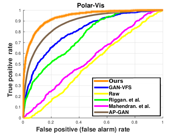
Regarding Protocol I, we evaluate and compare the performance of the proposed method with recent state-of-the-art methods [35, 19, 27, 26, 5, 36]. Figure 5 shows the evaluation performance for two different experimental settings, S0 (representing conventional thermal) and Polar separately. As can be seen from Figure 6, compared with the other state-of-the-art methods, the proposed method performs better and comparably to [36]. In addition, it can be observed that the performance corresponding to the Polar modality is always better than the S0 modality, which demonstrates the advantage of using the polarimetric thermal images than the conventional thermal images. The quantitative comparisons are shown in Table 1, and also demonstrate the effectiveness of the proposed method. Furthermore, Figure 6 shows some synthesized images. As can be seen from this figure, the facial attributes and the identity information is preserved well. Furthermore, from Figure 6(c) we see that the learned self-attention maps corresponding to both visible and thermal images are always located on the facial attributes regions such as mouth, eyes, and nose. As a result, the proposed self-attention guided GAN is able to capture meaningful information from both modalities for synthesis.
Table 2 compares the performance of several state-of-the-art image synthesis on Protocol II. These include multi-stream GAN [36], Pix2Pix [12], CycleGAN [39], and Pix2Pix-BEGAN [1]. Note that most prior works have not reported their results on Protocol II as it is based on a new extended dataset that was only recently made publicly available. Similar to Protocol I, the experiments are evaluated on two different settings - S0 and Polar separately. As can be seen from Table 2, the proposed method performs comparably to the most recent state-of-the art image synthesize algorithms. In this table, we also report the unsupervised performance of different methods. As expected, the supervised results outperform the unsupervised results with a large margin. Furthermore, the proposed method in unsupervised setting performs better than the other compared method. This clearly shows the significance of using self-attention module in our framework.
Note that a GAN-based multi-stream fusion method recently proposed in [36] is a supervised method that is specifically designed for the polarimetric data. The generator network consists of a multi-stream feature-level fusion encoder-decoder network. As a result, the performance of [36] is slightly better than our method on the polar modality. On the other hand, our method outperforms [36] by a large margin when only the S0 modality is used as the input. Our method can be viewed as a generic heterogeneous face recognition method. The performance of our method can be improved by using more sophisticated generators and feature extractors.
3.3 Ablation Study Regarding Fusion
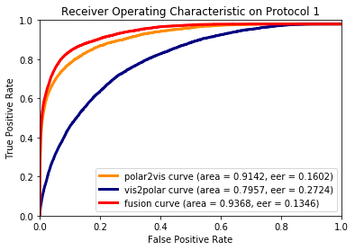
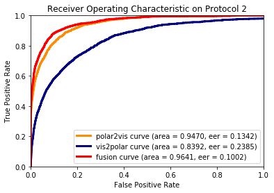
In this section, we analyze the effectiveness of using fusion features in our method. In this ablation study, given polar (thermal) images and visible images , we implement the following three experiments:
polar2vis: generate the visible images from the polar , then verify based on the features from .
vis2polar: generate the polar images from the visible , then verify based on the feature from .
fusion: generate the visible images from the polar and the polar images from the visible , then verify the images based on the features from .
This experiment will clearly show the significance of generating templates by fusing two features. The ablation study is evaluated on both Protocol I and Protocol II and the results are shown in Figure 7. Compared to the unimodal results, the fusion method significantly improves the performance on both protocols. Also, the visible modality outperforms than the polar modality due to the reason that the off-the-shelf VGGFace [23] feature extractor is pretrained on the visible face dataset.
4 Conclusion
We proposed a novel self-attention guided network for synthesizing thermal and visible faces for the task of cross-spectral face matching. Given visible probe images, we synthesize the corresponding thermal images. Similarly, given thermal probe images, we synthesize the visible images. Features are then extracted from the original and the synthesized images. Their fused feature representations are then used for verification. The generators are based on the self-attention guided networks. Various experiments on the ARL polarimetric thermal dataset were conducted to show the significance of the proposed approach. Furthermore, an ablation study was conducted to show the improvements achieved by the proposed fusion approach.
Though we have only evaluated our approach on polarimetric thermal to visible face verification, in the future, we will evaluate the performance of this method on other heterogeneous face recognition tasks such as sketch to face matching [32].
Acknowledgement
This work was supported by the Defense Forensics & Biometrics Agency (DFBA). The authors would like to thank Mr. Bill Zimmerman and Ms. Michelle Giorgilli for their guidance and extensive discussions on this work.
References
- [1] D. Berthelot, T. Schumm, and L. Metz. Began: boundary equilibrium generative adversarial networks. arXiv preprint arXiv:1703.10717, 2017.
- [2] T. Bourlai, N. Kalka, A. Ross, B. Cukic, and L. Hornak. Cross-spectral face verification in the short wave infrared (swir) band. In Pattern Recognition (ICPR), 2010 20th International Conference on, pages 1343–1347. IEEE, 2010.
- [3] J. Cheng, L. Dong, and M. Lapata. Long short-term memory-networks for machine reading. arXiv preprint arXiv:1601.06733, 2016.
- [4] X. Di, V. A. Sindagi, and V. M. Patel. Gp-gan: Gender preserving gan for synthesizing faces from landmarks. In 2018 24th International Conference on Pattern Recognition (ICPR), pages 1079–1084, Aug 2018.
- [5] X. Di, H. Zhang, and V. M. Patel. Polarimetric thermal to visible face verification via attribute preserved synthesis. IEEE International Conference on Biometrics: Theory, Applications, and Systems (BTAS), Oct. 2018.
- [6] I. Goodfellow, J. Pouget-Abadie, M. Mirza, B. Xu, D. Warde-Farley, S. Ozair, A. Courville, and Y. Bengio. Generative adversarial nets. In Advances in neural information processing systems, pages 2672–2680, 2014.
- [7] K. P. Gurton, A. J. Yuffa, and G. W. Videen. Enhanced facial recognition for thermal imagery using polarimetric imaging. Opt. Lett., 39(13):3857–3859, Jul 2014.
- [8] K. He, X. Zhang, S. Ren, and J. Sun. Deep residual learning for image recognition. In Proceedings of the IEEE conference on computer vision and pattern recognition, pages 770–778, 2016.
- [9] S. Hu, J. Choi, A. L. Chan, and W. R. Schwartz. Thermal-to-visible face recognition using partial least squares. JOSA A, 32(3):431–442, 2015.
- [10] S. Hu, N. J. Short, B. S. Riggan, C. Gordon, K. P. Gurton, M. Thielke, P. Gurram, and A. L. Chan. A polarimetric thermal database for face recognition research. In Proceedings of the IEEE Conference on Computer Vision and Pattern Recognition Workshops, pages 119–126, 2016.
- [11] S. M. Iranmanesh, A. Dabouei, H. Kazemi, and N. M. Nasrabadi. Deep cross polarimetric thermal-to-visible face recognition. In 2018 International Conference on Biometrics (ICB), pages 166–173, Feb 2018.
- [12] P. Isola, J.-Y. Zhu, T. Zhou, and A. A. Efros. Image-to-image translation with conditional adversarial networks. CVPR, 2017.
- [13] J. Johnson, A. Alahi, and L. Fei-Fei. Perceptual losses for real-time style transfer and super-resolution. In European Conference on Computer Vision, pages 694–711. Springer, 2016.
- [14] S. S. Y. L. S. D. Jonghyun Choi, Shuowen Hu. Thermal to visible face recognition. In Proc.SPIE, pages 8371 – 8371 – 10, 2012.
- [15] D. P. Kingma and J. Ba. Adam: A method for stochastic optimization. In International Conference on Learning Representations (ICLR), 2014.
- [16] B. Klare and A. K. Jain. Heterogeneous face recognition: Matching nir to visible light images. In Pattern Recognition (ICPR), 2010 20th International Conference on, pages 1513–1516. IEEE, 2010.
- [17] B. F. Klare and A. K. Jain. Heterogeneous face recognition using kernel prototype similarities. IEEE transactions on pattern analysis and machine intelligence, 35(6):1410–1422, 2013.
- [18] J. Lezama, Q. Qiu, and G. Sapiro. Not afraid of the dark: Nir-vis face recognition via cross-spectral hallucination and low-rank embedding. In 2017 IEEE Conference on Computer Vision and Pattern Recognition (CVPR), pages 6807–6816. IEEE, 2017.
- [19] A. Mahendran and A. Vedaldi. Understanding deep image representations by inverting them. In IEEE Conference on Computer Vision and Pattern Recognition, 2015.
- [20] T. Miyato, T. Kataoka, M. Koyama, and Y. Yoshida. Spectral normalization for generative adversarial networks. In International Conference on Learning Representations, 2018.
- [21] F. Nicolo and N. A. Schmid. Long range cross-spectral face recognition: matching swir against visible light images. IEEE Transactions on Information Forensics and Security, 7(6):1717–1726, 2012.
- [22] A. P. Parikh, O. Täckström, D. Das, and J. Uszkoreit. A decomposable attention model for natural language inference. In The Conference on Empirical Methods in Natural Language Processing, 2016.
- [23] O. M. Parkhi, A. Vedaldi, A. Zisserman, et al. Deep face recognition. In British Machine Vision Conference, 2015.
- [24] V. M. Patel, R. Gopalan, R. Li, and R. Chellappa. Visual domain adaptation: A survey of recent advances. IEEE Signal Processing Magazine, 32(3):53–69, May 2015.
- [25] B. S. Riggan, N. J. Short, and S. Hu. Optimal feature learning and discriminative framework for polarimetric thermal to visible face recognition. In 2016 IEEE Winter Conference on Applications of Computer Vision (WACV), pages 1–7. IEEE, 2016.
- [26] B. S. Riggan, N. J. Short, and S. Hu. Thermal to visible synthesis of face images using multiple regions. In IEEE Winter Conference on Applications of Computer Vision (WACV), 2018.
- [27] B. S. Riggan, N. J. Short, S. Hu, and H. Kwon. Estimation of visible spectrum faces from polarimetric thermal faces. In Biometrics Theory, Applications and Systems (BTAS), 2016 IEEE 8th International Conference on, pages 1–7. IEEE, 2016.
- [28] B. S. Riggan, N. J. Short, M. S. Sarfraz, S. Hu, H. Zhang, V. M. Patel, S. Rasnayaka, J. Li, T. Sim, S. M. Iranmanesh, and N. M. Nasrabadi. Icme grand challenge results on heterogeneous face recognition: Polarimetric thermal-to-visible matching. In 2018 IEEE International Conference on Multimedia Expo Workshops (ICMEW), pages 1–4, July 2018.
- [29] N. Short, S. Hu, P. Gurram, and K. Gurton. Exploiting polarization-state information for cross-spectrum face recognition. In Biometrics Theory, Applications and Systems (BTAS), 2015 IEEE 7th International Conference on, pages 1–6. IEEE, 2015.
- [30] N. Short, S. Hu, P. Gurram, K. Gurton, and A. Chan. Improving cross-modal face recognition using polarimetric imaging. Optics letters, 40(6):882–885, 2015.
- [31] A. Vaswani, N. Shazeer, N. Parmar, J. Uszkoreit, L. Jones, A. N. Gomez, Ł. Kaiser, and I. Polosukhin. Attention is all you need. In Advances in Neural Information Processing Systems, pages 5998–6008, 2017.
- [32] L. Wang, V. Sindagi, and V. Patel. High-quality facial photo-sketch synthesis using multi-adversarial networks. In 2018 13th IEEE International Conference on Automatic Face Gesture Recognition (FG 2018), pages 83–90, May 2018.
- [33] Z. Yi, P. Tan, and M. Gong. Dualgan: Unsupervised dual learning for image-to-image translation. In ICCV, 2017.
- [34] H. Zhang, I. Goodfellow, D. Metaxas, and A. Odena. Self-attention generative adversarial networks. arXiv preprint arXiv:1805.08318, 2018.
- [35] H. Zhang, V. M. Patel, B. S. Riggan, and S. Hu. Generative adversarial network-based synthesis of visible faces from polarimetrie thermal faces. In 2017 IEEE International Joint Conference on Biometrics (IJCB), pages 100–107, Oct 2017.
- [36] H. Zhang, B. S. Riggan, S. Hu, N. J. Short, and V. M. Patel. Synthesis of high-quality visible faces from polarimetric thermal faces using generative adversarial networks. International Journal of Computer Vision: Special Issue on Deep Learning for Face Analysis, 2019.
- [37] K. Zhang, Z. Zhang, Z. Li, and Y. Qiao. Joint face detection and alignment using multitask cascaded convolutional networks. IEEE Signal Processing Letters, 23(10):1499–1503, Oct 2016.
- [38] T. Zhang, A. Wiliem, S. Yang, and B. Lovell. Tv-gan: Generative adversarial network based thermal to visible face recognition. In 2018 International Conference on Biometrics (ICB), pages 174–181. IEEE, 2018.
- [39] J.-Y. Zhu, T. Park, P. Isola, and A. A. Efros. Unpaired image-to-image translation using cycle-consistent adversarial networkss. In Computer Vision (ICCV), 2017 IEEE International Conference on, 2017.