Learning Digital Camera Pipeline for Extreme Low-Light Imaging
Abstract
In low-light conditions, a conventional camera imaging pipeline produces sub-optimal images that are usually dark and noisy due to a low photon count and low signal-to-noise ratio (SNR). We present a data-driven approach that learns the desired properties of well-exposed images and reflects them in images that are captured in extremely low ambient light environments, thereby significantly improving the visual quality of these low-light images. We propose a new loss function that exploits the characteristics of both pixel-wise and perceptual metrics, enabling our deep neural network to learn the camera processing pipeline to transform the short-exposure, low-light RAW sensor data to well-exposed sRGB images. The results show that our method outperforms the state-of-the-art according to psychophysical tests as well as pixel-wise standard metrics and recent learning-based perceptual image quality measures.
1 Introduction
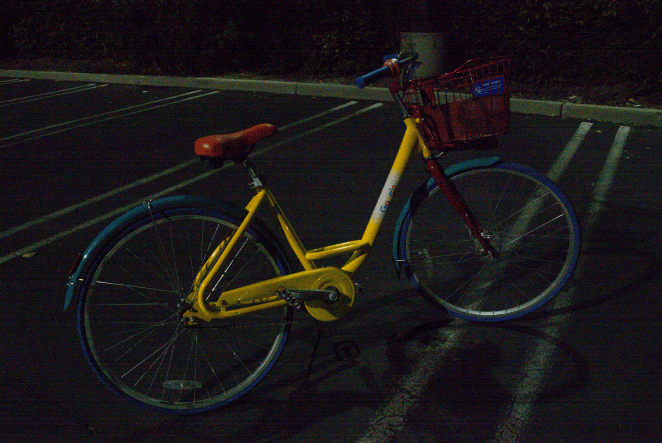
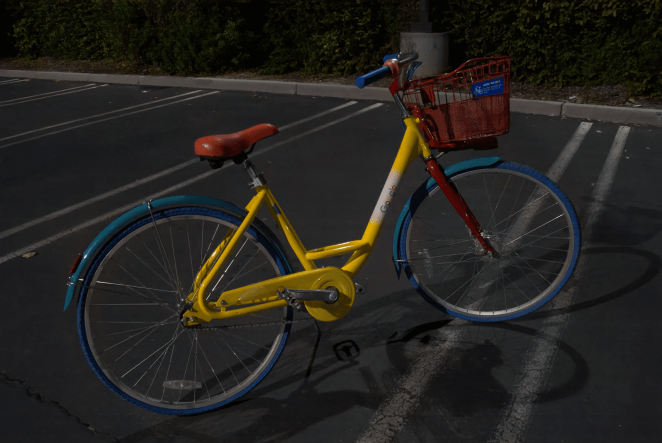
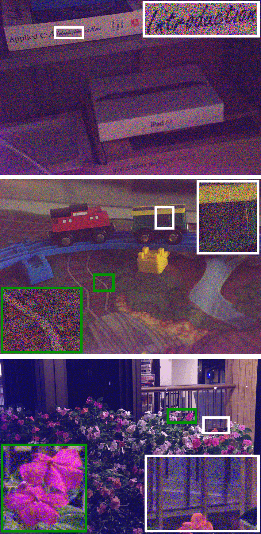
In a dark scene, the ambient light is not sufficient for cameras to accurately capture detail and color information. On one hand, leaving the camera sensor exposed to light for a long period of time retains the actual scene information, but may produce blurred images due to camera shake and object movement in the scene. On the other hand, images taken with a short exposure time preserve sharp details, but are usually dark and noisy. In order to address this dilemma, one might consider taking a sharp picture with a short exposure time and then increasing its brightness. However, the resulting image will not only have amplified noise and blotchy appearance, but the colors will also not match with those of a corresponding well-exposed image (see, for example, Figure 1b). Even if we reduce the problem of noise to some extent by using any state-of-the-art image denoising algorithm, the issue of color remains unsolved [1, 3].
A conventional camera imaging pipeline processes the RAW sensor data through a sequence of operations (such as white balance, demosaicking, denoising, color correction, tone mapping, sharpening, etc.) in order to generate the final RGB images [32]. Solving each of these problems requires hand-crafted priors and, even then, the pipeline breaks down in extremely low-light environments, often yielding dark images with little-to-no visible detail [3].
An alternative way to tackle the issue of low-light imaging is to use deep neural networks. These networks are data hungry in nature and require a large amount of training data: pairs of short-exposure input with corresponding long-exposure ground-truth. To encourage the development of learning-based techniques, Chen et al. [3] propose a large scale See-in-the-Dark (SID) dataset captured in low light conditions. The SID dataset contains both indoor and outdoor images acquired with two different cameras, having different color filter arrays. They further propose an end-to-end network, employing the loss, that learns the complete camera pipeline specifically for low-light imaging. However, the reproduced images often lack contrast and contain artifacts (see Figure 1c), especially under extreme low-light environments with severely limited illumination (e.g., dark room with indirect dim light source).
Most existing image transformation methods [3, 6, 23, 45] focus on measuring the difference between the network’s output and the ground-truth, using standard per-pixel loss functions. However, recent studies [16, 31, 46] have shown that applying traditional metrics (/, SSIM [41]) directly on the pixel-level information often provide overly smooth images that correlate poorly with human perception. These studies, therefore, recommend computing error on the deep feature representations, extracted from any pre-trained network [14, 19, 38], resulting in images that are visually sharp and perceptually faithful. A drawback of such a feature-level error computation strategy is the introduction of checkerboard artifacts at the pixel-level [16, 27]. Therefore, information from both the pixel-level and the feature-level is essential to produce images that are sharp, perceptually faithful and free from artifacts. The aforementioned observation motivates us to develop a new hybrid loss function, exploiting the basic properties of both pixel-wise and perceptual metrics.
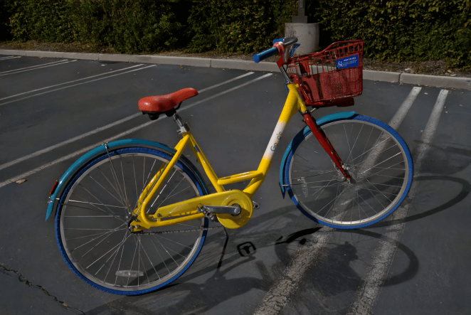
In this paper we propose a data-driven approach based on a novel loss function that is capable of generating well-exposed sRGB images with the desired attributes: sharpness, color vividness, good contrast, noise free, and no color artifacts. Our end-to-end network takes as input the RAW data captured in extreme low light and generates an sRGB image that fulfills these desired properties. By using our new loss function, we learn the entire camera processing pipeline in a supervised manner. Figure 1d shows the image produced by the proposed approach.
2 Background
Here, we first provide a brief overview of a traditional camera processing pipeline. We then discuss the recently introduced learning-based approach specifically designed for low-light imaging.
2.1 Traditional Camera Pipeline
The basic modules of the imaging pipeline, common to all standard single-sensor cameras, are the following [32]. (a) Preprocessing deals with the issues related to the RAW sensor data such as defective sensor cells, lens shading, light scattering and dark current. (b) White balance step estimates the scene illumination and remove its effect by linearly scaling the RAW data so that the reproduced image has no color cast [2, 17]. (c) Demosaicking stage takes in the RAW data, in which at each pixel location the information of only one color is present, and estimates the other two missing colors by interpolation [10], yielding a three-channel true color image. (d) Color correction transforms the image from the sensor-specific color space to linear sRGB color space [25]. (e) Gamma correction encodes images by allocating more bits to low luminance values than high luminance values, since we are more perceptible to changes in dark regions than bright areas. (f) Post processing stage applies several camera-specific (proprietary) operations to improve image quality, such as contrast enhancement [28], style and aesthetic adjustments [4, 15, 44], denoising [21, 30], and tone mapping [24]. Optionally, data compression may also be applied [40].

In low-light environments, the standard camera pipeline provides sub-optimal results due to a low photon count and SNR [1, 3]. To acquire well-exposed images in low light, apart from using long exposure, other methods include: exposure bracketing, burst imaging and fusion, larger-aperture lens, flash, and optical image stabilization [12]. However, each of these methods comes with a trade-off and is not always applicable. For instance, a mobile camera has thickness and power constraints, so adding a large lens with fast aperture is infeasible [12]. In exposure bracketing, a series of images are captured in quick succession with varying shutter speeds and then the user gets to pick the most visually pleasing image from this set, which oftentimes is none of them for difficult lighting. Image fusion for burst imaging often have misalignment problems, leading to ghosting artifacts. Finally, flash photography causes unwanted reflections, glare, shadows, and might change the scene illumination. In this paper, we address the problem of low light photography using single-imaging systems without flash.
2.2 Data-driven Image Restoration Approaches
Deep convolutional neural networks (CNNs) have been used with great success in ‘independently’ solving several image processing tasks such as denoising [21, 30], demosaicking [18], deblurring [26, 37, 43], super-resolution [6, 20, 47], inpainting [22, 29] and contrast enhancement [8, 39]. Recently, learning-based methods [3, 34] have been proposed that ‘jointly’ learn the complete camera processing pipeline in an end-to-end manner. Both of these methods take as input the RAW sensor data and produce sRGB images. Particularly, the work of Schwartz et al. [34] deals with images taken in well-lit conditions, and the method of Chen et al. [3] is developed specifically for extremely low-light imaging. After investigating several loss functions (, SSIM [41], total variation, and GAN [9]), Chen et al. [3] opt for a standard pixel-level loss function, i.e., , to measure the difference between the network’s prediction and the ground-truth. However, the per-pixel loss function is restrictive as it only models absolute errors and does not take into account the perceptual quality. Next, we propose an approach that exploits the characteristics of both pixel-wise and perceptual metrics to learn the camera processing pipeline in an end-to-end fashion.
3 Our Method
Our network design is based on a novel multi-criterion loss formulation, as shown in Figure 2. The model consists of two main blocks: (1) the ‘image restoration subnet’, and (2) the ‘perceptual loss subnet’. The image restoration subnet is an encoder-decoder architecture with skip connections between the contraction and expansion pathways. The perceptual loss subnet is a feed-forward CNN. Here, we first present the loss formulation and later describe each individual block in Sec. 3.2.
3.1 Proposed Multi-criterion Loss Function
As described earlier, the existing work [3] for low-light imaging is based on per-pixel loss, i.e., . We propose a multi-criterion loss function that jointly models the local and global properties of images using pixel-level image details as well as high-level image feature representations. Moreover, it explicitly incorporates perceptual similarity measures to ensure high-quality visual outputs.
Given an input image and the desired output image , the image restoration subnet learns a mapping function . The parameters are updated using the following multi-criterion loss formulation:
| (1) |
where, denotes the individual loss function, and are functions on the input and target image, respectively, whose definitions vary depending on the type of loss. In this paper, we consider two distinct representation levels (pixel-level and feature-level) to compute two loss criterion, i.e., . The first loss criterion, , is pixel-based and accounts for low-level image detail. The pixel-level loss is further divided into two terms: standard loss and structure similarity loss. The second loss criterion, , is a high-level perceptual loss based on intermediate deep feature representations. Next, we elaborate on these pixel-level and feature-level error criterion.
3.1.1 Pixel Loss:
The loss in Eq. (1) computes error directly on the pixel-level information of the network’s output and the ground-truth image. In this case, the definitions of and are fairly straight-forward: The loss function is defined as:
| (2) |
where is a weight parameter that we set using grid search on the validation set.
Absolute deviation.
The error directly minimizes the difference between the network output and the ground-truth to transform low-light images to well-exposed ones. Given and , the loss can be computed as:
| (3) |
where is the pixel location and denotes the total number of pixels in the image.
Although the metric is a popular choice for the loss function, it compromises high-frequency details, such as texture and sharp edges. To avoid such artifacts, we introduce a structural similarity measure in Eq. (2).
Structural similarity measure.
This term ensures the perceptual change in the structural content of output images to be minimal. In this work, we utilize the multi-scale structural similarity measure (MS-SSIM) [42]:
| (4) |
In order to define MS-SSIM, let us assume , and are the mean of image , the variance of , and the covariance of image and image , respectively. Then,
| (5) |
| (6) |
and finally,
| (7) |
where, is the number of scales. The first term in Eq. (7) compares the luminance of image with the luminance of reference image , and it is computed only at scale . The second term measures the contrast and structural differences at various scales. and adjust the relative importance of each term and, for convenience, we set for . and in Eq. (5) are small constants [42].
3.1.2 Feature Loss:
The pixel-level loss term is valuable for preserving original colors and detail in the reproduced images. However, it does not integrate perceptually sound global scene detail since the structural similarity is only enforced locally. To resolve this problem, we propose to use an additional loss term that quantifies the perceptual viability of the generated outputs in terms of a higher-order feature representation obtained from the perceptual loss subnet (see Figure 2).
In the feature loss term of the objective function (1), instead of calculating errors directly on the pixel-level, we measure the difference between the feature representations of the output and ground-truth images extracted with a deep network [36] pre-trained on the ImageNet dataset [5]. Note that this choice is motivated from a recent large-scale study [46] that demonstrates the suitability of deep features as a perceptual metric. In this case, the functions and are defined as , where denotes the layer activation map from the the network. The loss term is formulated as:
| (8) |
In this work, we use the VGG-16 network [36]. Note that other image classification networks such as AlexNet [19], ResNet [14], or GoogLeNet [38] can also be used to extract feature representations [46]. The perceptual loss function [16] enforces our image restoration subnet to generate outputs that are perceptually similar to their corresponding well-exposed reference images.
3.2 Network Architecture
Here we provide details of both blocks of our framework (see Figure 2).
Image restoration subnet. Our network inherits a U-net encoder-decoder structure [33] with symmetric skip connections between the lower layers of the encoder and the corresponding higher layers of the decoder. The benefits of such a design for the restoration subnet are three-fold: (a) it has superior performance on image restoration and segmentation tasks [3, 33], (b) it can process a full-resolution image (i.e., at or resolution) due to its fully convolutional design and low memory signature, and (c) the skip connections between the encoder and decoder modules enable adequate propagation of context information and preserve high-resolution details. Our network operates on RAW sensor data rather than RGB images, since our objective is to replace the traditional camera pipeline with an automatically learned network.
The image restoration subnet consists of a total of 23 convolutional layers. Among these, the encoder module has 10 convolutional layers, arranged as five pairs of layers. Each pair is followed by a leaky ReLU non-linearity and a max-pooling operator for subsampling. The decoder module has a total of 13 convolutional layers. These layers are arranged as a set of four blocks, each of which consists of a transpose convolutional layer whose output is concatenated with the corresponding features maps from the encoder module, followed by two convolutional layers. The number of channels in the feature maps are progressively reduced and the spatial resolution is increased due to the transpose convolutional layers. Finally, a convolutional layer, followed by a sub-pixel layer [35], is applied to remap the channels and obtain the RGB image with the same spatial resolution as the original RAW image. (For more details on network design and for a toy example, see supplementary material.)
Perceptual loss subnet.
The perceptual loss subnet consists of a truncated version of VGG-16 [36]. We only use the first two convolutional layers of VGG-16 and obtain the feature representation after ReLU non-linearity. This feature representation has been demonstrated to accurately encode the style and perceptual content of an image [16]. The result is a tensor for both the output of the image restoration net and the ground-truth, which are then used to compute the similarity between them.
4 Experiments
4.1 Dataset
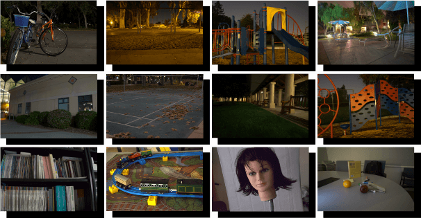
We validate our approach on the See-in-the-Dark (SID) dataset [3] that was specifically collected for the development of learning-based methods for low-light photography. In Figure 3 we show some sample images from the SID dataset. The images were captured using two different cameras: Sony 7S II with a Bayer color filter array (CFA) and sensor resolution of 42402832, and Fujifilm X-T2 with a X-Trans CFA and 60004000 spatial resolution. The dataset contains 5094 short-exposure RAW input images and their corresponding long-exposure reference images. Note that there are 424 unique long-exposure reference images, indicating that multiple short-exposure input images can correspond to the same ground-truth image. There are both indoor and outdoor images of the static scenes. The ambient illuminance reaching the camera was in the range 0.2 to 5 lux for outdoor scenes and between 0.03 lux and 0.3 lux for indoor scenes. Input images were taken with an exposure time between 1/30 and 1/10 seconds and the exposure time for the ground-truth images was 10 to 30 seconds.
4.2 Camera-specific Preprocessing
As mentioned in Sec. 2, cameras have a CFA in front of the image sensor to capture color information. Different cameras use different types of CFAs; Bayer filter array being the most popular choice due to its simple layout. Images of the SID dataset [3] come from cameras with different CFAs. Therefore, before passing the RAW input to the image restoration subnet (Figure 2), we pack the data, as in [3], into channels if it comes from Bayer CFA and channels for X-Trans CFA.
At the borders of the image sensor, there are some pixels that never see the light and therefore should be zero (black). However, during image acquisition, the values of these pixels are raised due to thermally generated voltage. We subtract this camera-specific black level from the image signal. Finally, we scale the sensor data with an amplification factor (e.g., 100, 250, or 300), which is the ratio between the reference image and the input image and determines the brightness of the output image.
4.3 Training
We train two separate networks: one for the Sony subset and the other for the Fuji subset from the SID dataset [3]. Each network takes as input a short-exposure RAW image and a corresponding long-exposure reference image (which is converted into the sRGB color space with the LibRAW library). Note that the input is prepared using camera-specific preprocessing mentioned in Sec. 4.2, before being passed through our network (Figure 2). Both networks are trained for epochs using the proposed loss function (Sec. 3.1). We use Adam optimizer with an initial learning rate of , which is reduced to after epochs. In each iteration we take a crop from the training image and perform random rotation and flipping. To compute the loss (8), we use features from the layer after ReLU of the VGG-16 network. The batch size is set to one, as we observed that setting the batch size greater than one reduces accuracy. This might be because the network struggles to learn, at once, the transformation process for images having significantly different light and noise levels. We empirically set and in Eq. (1) and Eq. (2), respectively, for all the experiments.
4.4 Qualitative Evaluation
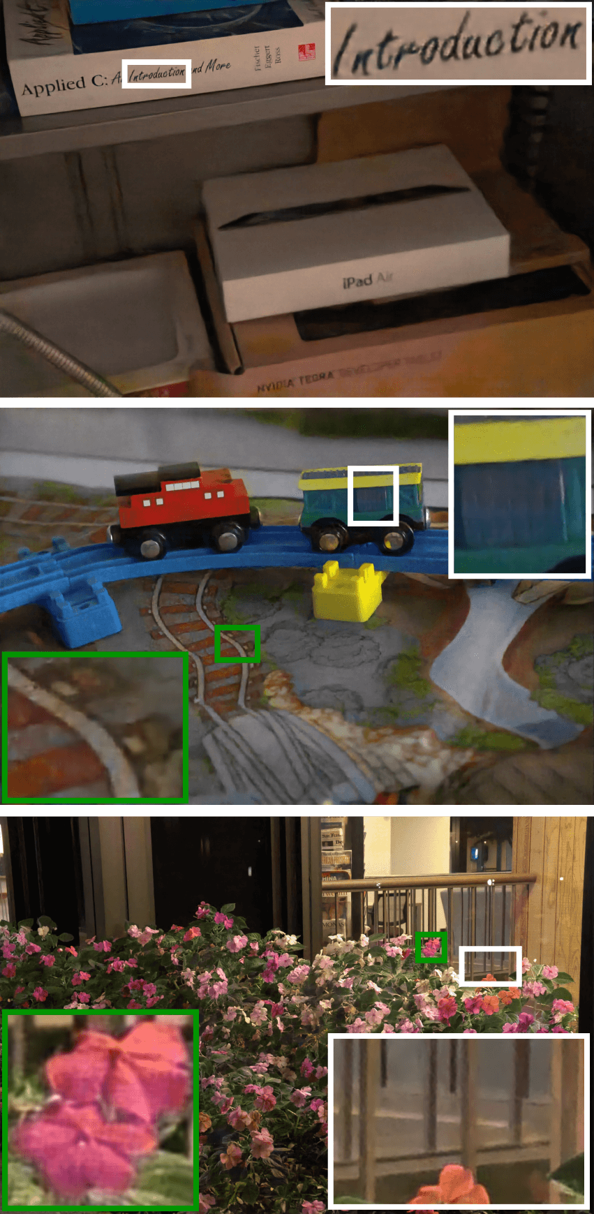
To the best of our knowledge, Chen et al. [3] present the “first and only” data-driven work that learns the digital camera pipeline specifically for extreme low-light imaging. Figure 4 presents a qualitative comparison of the images produced by our method and those of the state-of-the-art technique [3], as well as the traditional camera processing pipeline. Note that the traditional pipeline provides dark images with little-to-no visible detail. Therefore, we scale the brightness of the results of the traditional pipeline for visualization purposes. It is apparent in Figure 4(a) that the traditional pipeline handles low-light images poorly and yields results with extreme noise, color cast and artifacts. As reported in [1, 3], applying a state-of-the-art image denoising algorithm [11, 21, 30] might reduce noise to some extent. However, the issue of color distortion remains unsolved.
Figure 4 further shows that the results produced by our model are noticeably sharper, better denoised, more natural and visually pleasant, compared to those generated by the state-of-the-art method [3]. For instance, it can be seen in Figure 4(b) that the image reproductions of [3] exhibit splotchy textures (text, rail-track), color distortions (train, flowers, bottom corners of row 1) and poorly reconstructed shapes, such as for the text, rail-track and wooden fence.
Extremely challenging case.
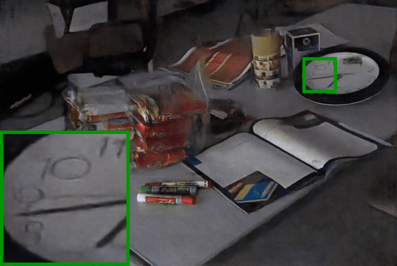
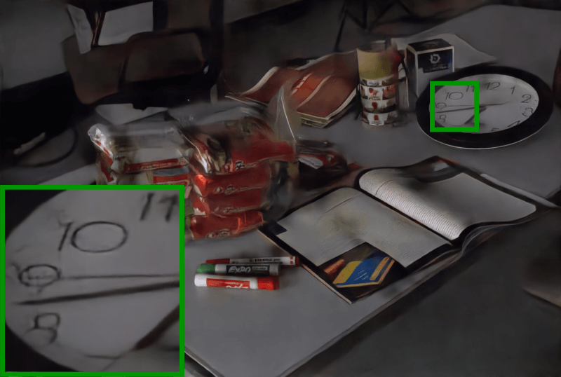
In Figure 5, we show the performance of our method on an (example) image captured in extremely difficult lighting: dark room with indirect dim light source. Our result might not be acceptable in isolation, but when compared with [3], we can greatly appreciate the reconstruction of sharp edges such as for the digits of the clock, and the spatial smoothness of the homogeneous regions, such as the table top and the floor.
| Experienced Observers | Inexperienced Observers | |||||
|---|---|---|---|---|---|---|
| x100 Set | x250 Set | x100 Set | x250 Set | |||
| Sony Dataset | Ours Chen et al. [3] | 84.7% | 92.6% | 80.3% | 86.6% | |
| Fuji Dataset | Ours Chen et al. [3] | 76.1% | 89.7% | 80.9% | 89.2% | |
| Sony subset [3] | Fuji subset [3] | ||||||
|---|---|---|---|---|---|---|---|
| PSNR | PieAPP [31] | LPIPS [46] | PSNR | PieAPP [31] | LPIPS [46] | ||
| Chen et al. [3] | 29.18 | 1.576 | 0.470 | 27.34 | 1.957 | 0.598 | |
| Ours | 29.43 | 1.511 | 0.443 | 27.63 | 1.763 | 0.476 | |
| (Chen et al. [3]) | MS-SSIM | + | + | ||||
|---|---|---|---|---|---|---|---|
| Sony subset [3] | 29.18 | 29.37 | 29.33 | 27.34 | 29.22 | 29.40 | 29.43 |
| Fuji subset [3] | 27.34 | 27.55 | 27.51 | 23.07 | 27.37 | 27.52 | 27.63 |
4.5 Subjective Evaluation of Perceptual Quality
We conduct a psychophysical experiment to assess the performance of competing approaches in an office-like environment. A corpus of 25 observers with normal color vision participated in the experiment. The subjects belong to two different groups: 7 expert observers with prior experience in image processing, and 18 naive observers. Each observer was shown a pair of corresponding images on the screen, sequentially and in random order: one of these images is produced by our method and the other one by Chen et al. [3]. Observers were asked to examine the color, texture, structure, sharpness and artifacts, and then choose the image which they find more pleasant. Each participant repeated this process on the test images of the Sony and Fuji subsets from the SID dataset [3]. The percentage with which the observers preferred images produced by our method than those of Chen et al. [3] is reported in Table 1. These results indicate that our method significantly outperforms the state-of-the-art [3] in terms of perceptual quality.
4.6 Quantitative Evaluation
To perform a quantitative assessment of the results, we use two recent learning-based perceptual metrics (LPIPS [46] and PieAPP [31]) and the standard PSNR metric. For the sake of fair comparison, we leave SSIM metric [41] out from the evaluation as our method is optimized using its variant MS-SSIM [42].
The average values of these metrics for the testing images of the Sony and Fuji subsets [3] are reported in Table 2.
Our method outperforms the state-of-the-art [3] by a considerable margin.
Ablation study.
The proposed loss function that minimizes the error of the network consists of three individual terms (, and ). Here, we evaluate the impact of each individual term and their combinations on our end-task. Table 3 summarizes our results where we compare different loss variants using the exact same parameter () settings. Our results demonstrate that each individual term contributes towards the final performance of our method. Based on the PSNR values in Table 3 and our qualitative observations, we draw the following conclusions: (a)
each individual component has its respective limitations e.g., yields colorful results but with artifacts, preserves fine image details but provides less saturated results, reconstructs structure well, but introduces checkerboard artifacts. (b) The combination of , and in an appropriate proportion provides the best results. The final loss function accumulates the complementary strengths of each individual criterion and avoids their respective shortcomings. The resulting images are colorful and artifact free, while faithfully preserving image structure and texture 111Additional results are provided in supplementary material..
5 Contrast Improvement Procedure
The network of Chen et al. [3] produces images that are often dark and lack contrast. It is the inherent limitation enforced by the imperfect ground-truth of the SID dataset, and therefore learned network will also be only partially optimal. In attempt to dealing with this issue, [3] preprocesses the ground-truth images with histogram equalization. Subsequently, their network learns to generate contrast enhanced outputs; however, with artifacts. Thus the performance of the method [3] was significantly reduced.
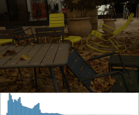
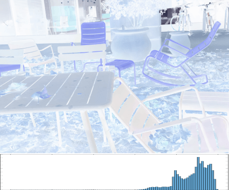
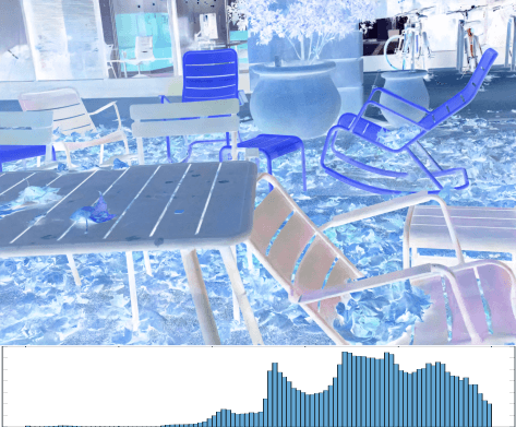
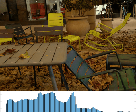
Inspired from [7], we employ the following procedure in order to improve the color contrast of the results produced by our proposed method. We observe that the histogram of outputs produced by our image restoration subnet is mostly skewed towards dark regions (see for example Figure 6(a)). By inverting the intensity values of the image, the histogram becomes similar to that of a hazy image (Figure 6(b)). This indicates that, by applying an image dehazing algorithm [13], we can make the image histogram more uniform (Figure 6(c)). Finally, inverting back the intensities of the image provides us with a new image that is bright, sharp, colorful and without artifacts, as shown in Figure 6(d).
We notice that preprocessing the reference images by applying the just mentioned procedure and then training the network from scratch produces suboptimal results. Therefore, we first train the network with regular ground-truth for 4000 epochs, and then perform fine-tuning for another 100 epochs with the contrast-enhanced ground-truth.
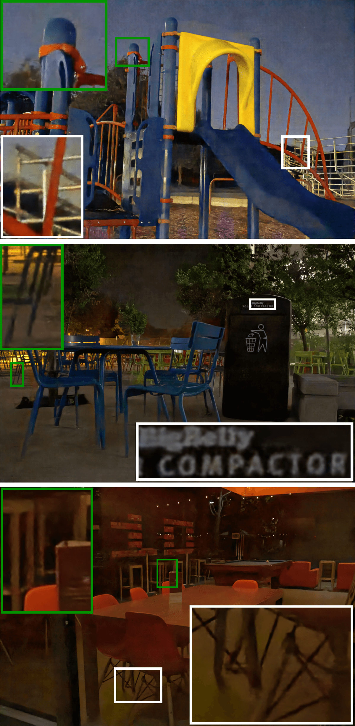
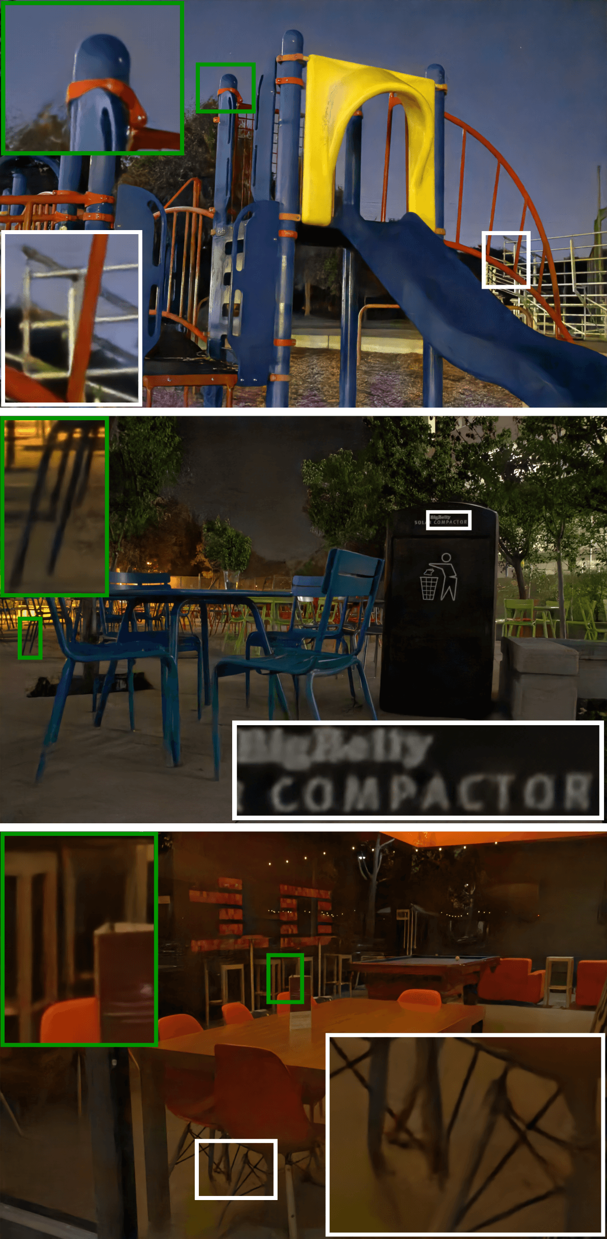
In Figure 7, we compare the results obtained after applying the contrast improvement strategy to our image restoration net and to the framework of Chen et al. [3]. It is evident that our method produces visually compelling images with good contrast and vivid colors. Whereas the method of [3] has a tendency of reproducing images with artifacts, which become even more prominent when the contrast enhancement procedure is employed; notice the zoomed-in portions of Figure 7, especially the sky in column 1.
6 Conclusion
Imaging in extremely low-light conditions is a highly challenging task for the conventional camera pipeline, often yielding dark and noisy images with little-to-no detail. In this paper, we proposed a learning-based approach that learns the entire camera pipeline, end-to-end, for low-light conditions. We explored the benefits of computing loss both at the pixel-level information and at the feature-level, and presented a new loss function that significantly improved the performance. We conducted a psychophysical study, according to which the observers overwhelmingly preferred the outputs of our method over the existing state-of-the-art. Similar trends were observed when the image quality of the competing methods was assessed with standard metrics, as well as recent learning-based error metrics.
References
- [1] M. Bertalmío and S. Levine. Variational approach for the fusion of exposure bracketed pairs. TIP, 22(2):712–723, 2013.
- [2] G. Buchsbaum. A spatial processor model for object colour perception. Journal of the Franklin Institute, 310(1):1 – 26, 1980.
- [3] C. Chen, Q. Chen, J. Xu, and V. Koltun. Learning to see in the dark. In CVPR, 2018.
- [4] Q. Chen, J. Xu, and V. Koltun. Fast image processing with fully-convolutional networks. In ICCV, 2017.
- [5] J. Deng, W. Dong, R. Socher, L. Li, K. Li, and L. Fei-Fei. ImageNet: A large-scale hierarchical image database. In CVPR, 2009.
- [6] C. Dong, C. C. Loy, K. He, and X. Tang. Image super-resolution using deep convolutional networks. TPAMI, 38(2):295–307, 2016.
- [7] X. Dong, G. Wang, Y. Pang, W. Li, M. W. Wen, J., and Y. Lu. Fast efficient algorithm for enhancement of low lighting video. In ICME, pages 1–6, 2011.
- [8] M. Gharbi, J. Chen, J. T. Barron, S. W. Hasinoff, and F. Durand. Deep bilateral learning for real-time image enhancement. TOG, 36(4):118, 2017.
- [9] I. Goodfellow, J. Pouget-Abadie, M. Mirza, B. Xu, D. Warde-Farley, S. Ozair, A. Courville, and Y. Bengio. Generative adversarial nets. In NIPs, 2014.
- [10] B. K. Gunturk, J. Glotzbach, Y. Altunbasak, R. W. Schafer, and R. M. Mersereau. Demosaicking: color filter array interpolation. IEEE Signal Processing Magazine, 22(1):44–54, 2005.
- [11] S. Guo, Z. Yan, K. Zhang, W. Zuo, and L. Zhang. Toward convolutional blind denoising of real photographs. arXiv preprint arXiv:1807.04686, 2018.
- [12] S. W. Hasinoff, D. Sharlet, R. Geiss, A. Adams, J. T. Barron, F. Kainz, J. Chen, and M. Levoy. Burst photography for high dynamic range and low-light imaging on mobile cameras. TOG, 35(6):192, 2016.
- [13] K. He, J. Sun, and X. Tang. Single image haze removal using dark channel prior. TPAMI, 33(12):2341–2353, 2011.
- [14] K. He, X. Zhang, S. Ren, and J. Sun. Deep residual learning for image recognition. In CVPR, 2016.
- [15] M. He, D. Chen, J. Liao, P. V. Sander, and L. Yuan. Deep exemplar-based colorization. TOG, 37(4):47, 2018.
- [16] J. Johnson, A. Alahi, and L. Fei-Fei. Perceptual losses for real-time style transfer and super-resolution. In ECCV, 2016.
- [17] H. C. Karaimer and M. S. Brown. Improving color reproduction accuracy on cameras. In CVPR, 2018.
- [18] F. Kokkinos and S. Lefkimmiatis. Deep image demosaicking using a cascade of convolutional residual denoising networks. In ECCV, 2018.
- [19] A. Krizhevsky, I. Sutskever, and G. E. Hinton. ImageNet classification with deep convolutional neural networks. In NIPS, 2012.
- [20] W.-S. Lai, J.-B. Huang, N. Ahuja, and M.-H. Yang. Deep laplacian pyramid networks for fast and accurate superresolution. In CVPR, 2017.
- [21] S. Lefkimmiatis. Universal denoising networks: A novel CNN architecture for image denoising. In CVPR, 2018.
- [22] G. Liu, F. A. Reda, K. J. Shih, T.-C. Wang, A. Tao, and B. Catanzaro. Image inpainting for irregular holes using partial convolutions. In ECCV, 2018.
- [23] J. Long, E. Shelhamer, and T. Darrell. Fully convolutional networks for semantic segmentation. In CVPR, 2015.
- [24] R. Mantiuk, S. Daly, and L. Kerofsky. Display adaptive tone mapping. TOG, 27(3):1–10, 2008.
- [25] J. Morovič. Color gamut mapping, volume 10. Wiley, 2008.
- [26] S. Nah, T. H. Kim, and K. M. Lee. Deep multi-scale convolutional neural network for dynamic scene deblurring. In CVPR, 2017.
- [27] A. Odena, V. Dumoulin, and C. Olah. Deconvolution and checkerboard artifacts. Distill, 2016.
- [28] R. Palma-Amestoy, E. Provenzi, M. Bertalmío, and V. Caselles. A perceptually inspired variational framework for color enhancement. TPAMI, 31(3):458–474, 2009.
- [29] D. Pathak, P. Krahenbuhl, J. Donahue, T. Darrell, and A. A. Efros. Context encoders: Feature learning by inpainting. In CVPR, 2016.
- [30] T. Plotz and S. Roth. Benchmarking denoising algorithms with real photographs. In CVPR, 2017.
- [31] E. Prashnani, H. Cai, Y. Mostofi, and P. Sen. PieAPP: Perceptual image-error assessment through pairwise preference. In CVPR, 2018.
- [32] R. Ramanath, W. E. Snyder, Y. Yoo, and M. S. Drew. Color image processing pipeline. IEEE Signal Processing Magazine, 22(1):34–43, 2005.
- [33] O. Ronneberger, P. Fischer, and T. Brox. U-net: Convolutional networks for biomedical image segmentation. In MICCAI, 2015.
- [34] E. Schwartz, R. Giryes, and A. M. Bronstein. DeepISP: Towards learning an end-to-end image processing pipeline. TIP, 2018. (Early Access).
- [35] W. Shi, J. Caballero, F. Huszár, J. Totz, A. P. Aitken, R. Bishop, D. Rueckert, and Z. Wang. Real-time single image and video super-resolution using an efficient sub-pixel convolutional neural network. In CVPR, 2016.
- [36] K. Simonyan and A. Zisserman. Very deep convolutional networks for large-scale image recognition. In ICLR, 2015.
- [37] S. Su, M. Delbracio, J. Wang, G. Sapiro, W. Heidrich, and O. Wang. Deep video deblurring for hand-held cameras. In CVPR, 2017.
- [38] C. Szegedy, W. Liu, Y. Jia, P. Sermanet, S. Reed, D. Anguelov, D. Erhan, V. Vanhoucke, and A. Rabinovich. Going deeper with convolutions. In CVPR, 2015.
- [39] H. Talebi and P. Milanfar. Learned perceptual image enhancement. In ICCP, 2018.
- [40] G. K. Wallace. The JPEG still picture compression standard. ACM - Special issue on digital multimedia Commun., 34(4):30–44, 1991.
- [41] Z. Wang, A. C. Bovik, H. R. Sheikh, and E. P. Simoncelli. Image quality assessment: from error visibility to structural similarity. TIP, 13(4):600–612, 2004.
- [42] Z. Wang, E. P. Simoncelli, and A. C. Bovik. Multiscale structural similarity for image quality assessment. In ACSSC, 2003.
- [43] L. Xu, J. S. J. Ren, C. Liu, and J. Jia. Deep convolutional neural network for image deconvolution. In NIPS, 2014.
- [44] Z. Yan, H. Zhang, B. Wang, S. Paris, and Y. Yu. Automatic photo adjustment using deep neural networks. TOG, 35(2):1–15, 2016.
- [45] R. Zhang, P. Isola, and A. A. Efros. Colorful image colorization. In ECCV, 2016.
- [46] R. Zhang, P. Isola, A. A. Efros, E. Shechtman, and O. Wang. The unreasonable effectiveness of deep features as a perceptual metric. In CVPR, 2018.
- [47] Y. Zhang, K. Li, K. Li, L. Wang, B. Zhong, and Y. Fu. Image super-resolution using very deep residual channel attention networks. In ECCV, 2018.

