Impact of Pulsar and Fallback Sources on Multifrequency Kilonova Models

Abstract

We explore the impact of pulsar electromagnetic dipole and fallback accretion emission on the luminosity of a suite of kilonova models. The pulsar models are varied over pulsar magnetic field strength, pulsar lifetime, ejecta mass, and elemental abundances; the fallback models are varied over fallback accretion rate and ejecta mass. For the abundances, we use Fe and Nd as representatives of the wind and dynamical ejecta, respectively. We simulate radiative transfer in the ejecta in either 1D spherical or 2D cylindrical spatial geometry. For the grid of 1D simulations, the mass fraction of Nd is 0, $10^{-4}$, or $10^{-3}$ and the rest is Fe. Our models that fit the bolometric luminosity of AT 2017gfo (the kilonova associated with the first neutron star merger discovered in gravitational waves, GW170817) do not simultaneously fit the B, V, and I time evolution. However, we find that the trends of the evolution in B and V magnitudes are better matched by the fallback model relative to the pulsar model, implying the time dependence of the remnant source influences the color evolution. Further exploration of the parameter space and model deficiencies is needed before we can describe AT 2017gfo with a remnant source.

1. Introduction

Under the standard accretion disk paradigm for gamma-ray bursts, the outflow is powered by the release of accretion energy, typically assumed to be driven by magnetic fields. Bursts were distinguished by their duration and hardness (Kouveliotou et al., 1993). The burst duration in the accretion disk paradigm corresponds to the disk accretion timescale which, in turn, corresponds to different progenitors (Popham et al., 1999): long bursts are believed to be produced in systems where the disk can be continuously fed (e.g. collapse of massive stars) whereas short bursts are believed to be produced by compact disks (e.g. mergers of compact binaries). With these predictions for different progenitors for different bursts, theorists were able to argue for different properties of short and long bursts with respect to their locations in their host galaxies (Bloom et al., 1999; Fryer et al., 1999). Observations confirmed the distribution of locations (Fong & Berger, 2013), verifying both the compact binary progenitor and the accretion disk paradigm. Neutron star/neutron star (NS/NS) and neutron star/black hole (NS/BH) mergers are the most likely compact mergers behind these short bursts.

These compact mergers have also been invoked as the source of r-process elements, the dynamically ejected material is so neutron rich that it produces a robust heavy r-process yield. Initially proposed over 4 decades ago (Lattimer & Schramm, 1974), increasingly detailed studies support this as a leading source of r-process elements (e.g. Freiburghaus et al., 1999; Korobkin et al., 2012; Bauswein et al., 2013; Lippuner & Roberts, 2015; Radice et al., 2016; Thielemann et al., 2017). For a review on the role of mergers in r-process production, see (Côté et al., 2018). The merger also forms a disk of high angular momentum material that drives outflows while accreting onto the central compact object. This late-time outflow ejecta is bathed in neutrinos and is likely to be less neutron rich, producing lighter (first peak r-process, iron peak) elements (Metzger & Fernández, 2014). With the broadband and multi-messenger detection of GW170817 (Abbott et al., 2017c, b, a), astronomers were able to make the first definitive detection of a neutron star merger with gravitational wave (GW) measurements providing proof of (and constraints on) the merger, gamma-ray, X-ray and radio measurements of what appears to be a gamma-ray burst jet and UVOIR measurements of the merger ejecta.

With these UVOIR measurements, astronomers can, for the first time, place observed constraints on the r-process production in a neutron star merger. Moreover, these observations place constraints on nuclear composition, and hence nuclear mass models beyond the standard abundance curve (Mumpower et al., 2016). The standard models for the UVOIR emission assume a broad range of ejecta including both neutron-rich dynamical ejecta (producing heavy r-process, including lanthanides that have high optical opacities) as well as lighter elements produced by the higher electron-fraction ejecta during the accretion of the disk. The radioactive decay of these elements powers a supernova-like light curve (kilonova) and, by comparing this emission to the observations, astronomers can estimate the mass of the ejecta. The analysis of the emission to determine the exact ejecta from this merger depends upon the opacities, the opacity implementation and the distribution of this ejecta, i.e. composition, density, and velocity as a function of position (radius and angle). Models ranged from constant opacity implementations to full lanthanide opacities (utilizing a few representative isotopes) and distributions ranging from spherical mixes to multi-component ejecta models. None of the models capture all the physics and they predict a range of ejecta masses that from the observations that varies by an order of magnitude (Côté et al., 2018).

If these uncertainties were not enough, additional power sources could be augmenting the energy released from nuclear decay. As the accretion rate lowers, the radiation from the material accreting on the merged compact object is no longer trapped in the inflow and it can augment the power of the burst. In addition, there is some evidence that the merged core could be a magnetized neutron star (Li et al., 2018; Piro et al., 2018). A normal, few times $10^{11}-10^{12}{\rm G}$ pulsar could power the light curve. Higher remnant magnetic fields, $\sim 10^{14}-10^{16}$ G, have also been explored, and can produce luminosity well into supernova range for $10^{-4}-10^{-2}$ M_⊙ (Yu et al., 2013; Metzger & Piro, 2014). Alternatively, fallback (Li et al., 2018; Matsumoto et al., 2018) and cocoon emission (Kasliwal et al., 2017; Matsumoto et al., 2018) have been invoked as supplying additional power to the light curve of GW170817, on top of heating from r-process decay. Similarly for GRB 130603B, motivated by the observed X-ray excess, a central X-ray emission source undergoing reprocessing to the infrared has been used to lower ejecta mass estimates from the IR excess (Kisaka et al., 2016).

In this paper, we present a grid of models to study the features of pulsar and fallback accretion energy sources. The outline of our models are given in Section 2. Section 2.1 describes the 1- and 2-dimensional models used in our calculations, Section 2.2 describes our remnant sources (pulsar and accretion) and Section 2.3 describes the simulation methods used to produce kilonova light curves. With our grid of models, we produce a broad range of light curves and spectra (Section  3). Although we compare these to observations of GW170817, the intent of this project is to provide a database of spectra and light curves for upcoming observations.

2. Model Properties and Simulations

2.1. Ejecta Profiles

For this project, we use both 1- and 2-dimensional outflow models. To initialize the 1D spherical ejecta, we use a slight modification to the semi-analytic, homologous solution discussed in Section 2.1.1 of Wollaeger et al. (2018),

$$v(r,t)=\frac{r}{t}\;\;,$$ (1a)

$$\rho(r,t)=\rho_{0}\left(\frac{t}{t_{0}}\right)^{-3}\left(1-\frac{r^{2}}{(v_{\max}t)^{2}}\right)^{3}\;\;,$$ (1b)

$$\mathcal{E}(r,t)=\mathcal{E}_{0}\left(\frac{t}{t_{0}}\right)^{-4}\left(1-\frac{r^{2}}{(v_{\max}t)^{2}}\right)^{4}+E_{\rm source}(t)\frac{\delta(r)}{4\pi r^{2}}\;\;,$$ (1c)

where $r$, $v$, $\rho$, $\mathcal{E}$, $t_{0}$, and $v_{\max}$ are radius, velocity, density, radiation energy density, initial time, and maximum velocity, respectively. The value of $\mathcal{E}_{0}$ accounts for the contribution of r-process nucleosynthesis and heating to the initial internal energy of the ejecta, and is the same value used by Wollaeger et al. (2018). The value $E_{\rm source}$ is the energy contribution from a source near the compact remnant (either from pulsar luminosity or accretion energy). We will discuss this source in more detail in section 2.2. The composition of this material is assumed to be either dominated by iron peak elements using Fe for the opacity or mostly dominated by iron peak elements with trace amounts of heavy r-process where lanthanide opacities are the most critical (with a mass fraction of $10^{-4}$ or $10^{-3}$ in Nd to represent lanthanides). For the ejecta, we adopt masses and velocities similar to the models of Li et al. (2018).

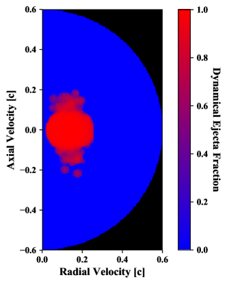
We also include a suite of models assuming a 2-component ejecta model in 2D cylindrical geometry, superimposing the spherically symmetric wind described above onto the “model A” dynamical ejecta of the SPH simulations by Rosswog et al. (2014) (see also Rosswog (2013)). This is similar to the 2-component models of Wollaeger et al. (2018) , though their wind velocity and mass are lower and higher, respectively, following the simulations of Perego et al. (2014). The model A dynamical ejecta was derived from the simulation of the merger of two 1.4 M_⊙ neutron stars, which produced an ejected mass of 0.013 M_⊙ (Rosswog et al., 2014). For the simulations in SuperNu, this ejecta has been mapped to an axisymmetric 2D grid; hence the 3D variations around the merger axis are lost. For the wind composition, we use the same abundance options as in our 1-dimensional models, Fe. For the dynamical ejecta, we use Nd to represent a lanthanide-rich ejecta. The Model A ejecta proved to have an unobscured region permitting viewing angles where a blue wind transient can manifest (Wollaeger et al., 2018). Consequently, the viewing-angle dependence of the light curves and spectra from this model permits the effect of the remnant luminosity to be observed at different degrees of obscurity. Figure 1 has dynamical ejecta fraction at each velocity coordinate, where it is colored red where dynamical ejecta dominates, blue where wind ejecta dominates and black where there is no ejecta. The fast wind can be seen to completely surround the dynamical ejecta, but is of relatively low density. Half of the wind mass is within a radius of $0.3c$, and the remnant source is always at the origin. We have not explored non-spherical wind morphologies, which may affect the expression of the remnant source in the blue kilonova.

Figure 1.— Fraction of dynamical ejecta at each point in the 2D morphology. The dynamical ejecta component (red) is from Rosswog et al. (2014) and the spherical wind component (blue) is from Eq. (1) (Wollaeger et al., 2018).

2.2. Remnant Sources Enhancing the Kilonova Emission

In most kilonova light-curve models, the emission is powered by the decay of radioactive isotopes. For our models, we include this energy, but we also include the energy from an active remnant region: either pulsar or accretion luminosity. At early times, this energy is trapped in the outflowing ejecta and we can treat it as an energy source, i.e. $E_{\rm source}$ in Eq. (1). Consequently, we initialize our radiative transfer simulations by solving for $E_{\rm source}$ at $t_{0}$, assuming the energy balance is determined by adiabatic cooling and energy injection from the remnant source. After our initialization, the evolution of $\mathcal{E}(r,t)$ is fully determined by radiative transfer. Let’s review the features of our pulsar and accretion luminosities, and how the initial value of $E_{\rm source}$ is calculated.

2.2.1 Pulsar Luminosity

Especially in newly formed neutron stars like the merged compact object in NS/NS binaries, pulsar emission can vary due to magnetic field restructuring, high-order field configurations, etc. Here we assume a simple dipole magnetic field source with a constant magnetic field following the pulsar luminosity formulae explored in recent studies (Lasky & Glampedakis, 2016; Li et al., 2018; Piro et al., 2018). Following Lasky & Glampedakis (2016), the loss of neutron star remnant angular kinetic energy is balanced by EM dipole and GW quadrupole luminosity,

$$-I\Omega\dot{\Omega}=\frac{B_{p}^{2}R^{6}\Omega^{4}}{6c^{3}}+\frac{32GI^{2}\epsilon^{2}\Omega^{6}}{5c^{2}}\;\;,$$ (2)

where the variables are defined by Lasky & Glampedakis (2016). The pulsar luminosity is given as the electromagnetic (EM) dipole luminosity multiplied by an efficiency parameter, $\eta$, corresponding to the radiation beaming angle (Rowlinson et al., 2014; Lasky & Glampedakis, 2016). Assuming GW dominated spin-down, the luminosity is (Lasky & Glampedakis, 2016)

$$L_{d}(t)=\frac{\eta B_{p}^{2}R^{6}\Omega(t)^{4}}{6c^{3}}=L_{0}\left(1+\frac{t}{t_{\rm gw}}\right)^{-1}\;\;,$$ (3)

where

$$L_{0}=\frac{\eta\Omega_{0}^{4}B_{p}^{2}R^{6}}{6c^{3}}\;\;,$$ (4a)

$$t_{\rm gw}=\frac{5c^{5}}{128GI\epsilon^{2}\Omega_{0}^{4}}\;\;.$$ (4b)

To explore the effect of variable remnant lifetime, we introduce a time cut-off, $t_{\rm cut}$, to the luminosity,

$$L_{d}(t)=L_{0}\left(1+\frac{t}{t_{\rm gw}}\right)^{-1}\Theta(t_{\rm cut}-t)\;\;,$$ (5)

where $\Theta$ is the unit step function.

The energy source $E_{\rm source}$ in Eq. (1) for our pulsar models can then be written as:

$$\dot{E}_{\rm source}=-\frac{E_{\rm source}}{t}+L_{d}\;\;,$$ (6)

where $L_{d}$ is given from Eq. (5) and $E_{d}(0)=0$. Note Eq. (6) is a simplification of the ejecta layer equations given by Metzger (2017), neglecting diffusion and changes to the inner velocity from the impulse of the pulsar luminosity. Thus we have assumed that the pulsar luminosity is not high enough to significantly impact the morphology of the ejecta. The solution to Eq. (6) is

$$E_{\rm source}(t)=L_{0}\frac{t_{\rm gw}}{t}\left[t^{\prime}-t_{\rm gw}\ln\left(\frac{t^{\prime}+t_{\rm gw}}{t_{\rm gw}}\right)\right]\;\;,$$ (7)

where $t^{\prime}=\min(t,t_{\rm cut})$; the derivative with respect to $t^{\prime}/t_{\rm gw}$ of the term in braces is always positive, showing $E_{d}(t)\geq 0$.

In our simulations, $E_{d}(t_{0})$ is added to the innermost spatial cell at a start time of $t_{0}$. If $t_{\rm cut}>t_{0}$, the pulsar is still active during the simulation, and Eq. (5) is integrated over each time step to add further energy to the innermost cell. In all simulations, we use $t_{0}=10^{4}$ s.

2.2.2 Fallback Luminosity

Another source of energy can come from fallback after the initial kilonova explosion. Fallback in stellar outbursts follows a simple power law with time ($\dot{m}\propto t^{-5/3}$ where $\dot{m}$ is the fallback accretion rate and $t$ is the time) (Chevalier, 1989). The energy and mass ejected is more complex and high-resolution models have been studied in the case of supernova fallback (Fryer, 2009). These models showed that roughly $\sim$10-25% of the fallback matter is re-ejected, carrying away roughly 10-25% of the accretion energy. These properties are directly applicable to the fallback in this scenario and is similar to the simple prescriptions used in the kilonova community, e.g., Li et al. (2018):

$$L_{f}(t)=\frac{\eta}{\eta_{r}}L_{0}\left(\frac{\dot{m}_{0}}{\dot{m}_{r}}\right)\left(\frac{t}{t_{\rm acc}}\right)^{-5/3}=\tilde{L}_{0}\left(\frac{t}{t_{\rm acc}}\right)^{-5/3}\;\;,$$ (8)

where $\eta$ is again an efficiency parameter (roughly 10-25%), $t_{\rm acc}$ is initial time (when the luminosity begins to fall off), $\dot{m}_{0}$ is the initial accretion rate, and $\dot{m_{r}}$ is a reference accretion rate. Reference values $\eta_{r}$ and $\dot{m}_{r}$ are taken to be 0.1 and $10^{-3}$ M_⊙/s, respectively.

As with our pulsar emission, we do not modify the ejecta mass or momentum in our outflow, focusing instead on the energy injected from this accretion. This luminosity corresponds to a source energy of

$$\dot{E}_{\rm source}=-\frac{E_{\rm source}}{t}+L_{\rm fallback}\;\;,$$ (9)

and $L_{\rm fallback}$ is given by Eq. (8). Assuming the luminosity is proportional to $t^{-5/3}$ back to $t_{\rm acc}$, then $E_{\rm source}$ can be solved analytically from Eq. (9). We assume the luminosity $t^{-5/3}$ dependence holds as early as $t_{\rm acc}$ (which may only be true at $t\gg t_{\rm acc}$ (Metzger, 2017)). Assuming the fallback luminosity is constant before $t_{\rm acc}$, the solution is

$$E_{\rm source}=\begin{cases}\displaystyle\tilde{L}_{0}\frac{t_{\rm acc}^{2}}{2t}+\tilde{L}_{0}t_{\rm acc}^{5/3}\left(\frac{1}{t^{2/3}}-\frac{t_{\rm acc}^{1/3}}{t}\right)\;\;,\;\;t>t_{\rm acc}\;\;,\\ \displaystyle\frac{t_{\rm acc}\tilde{L}_{0}}{2}\;\;,\;\;t\leq t_{\rm acc}\;\;.\end{cases}$$ (10)

Unlike the pulsar models, we do not introduce a cut-off time for the source.

For the fallback models, a considerable amount of energy can be injected into the ejecta on short time scales. Adopting parameters similar to Li et al. (2018), $\eta=0.1$, $L_{0}=2\times 10^{51}$ erg/s, and $\dot{m}_{0}=10^{-3}$ M_⊙/s, from Eq. (10), the energy added up to $t_{\rm acc}$ is $10^{50}$ erg. The kinetic energy of our smallest-mass ejecta is $\sim M_{\rm ej}(v_{\max}/2)^{2}/2\approx 10^{50}$ erg. Assuming all the energy before $t_{\rm acc}$ goes into boosting the kinetic energy, the resulting average velocity should be increased to about $\tilde{v}_{\max}/2=\sqrt{2}v_{\max}/2\approx 0.42c$. Consequently, we also simulate a suite of fallback kilonova models with $v_{\max}/2=0.45$ and with

$$E_{\rm source}=\begin{cases}\displaystyle\tilde{L}_{0}t_{\rm acc}^{5/3}\left(\frac{1}{t^{2/3}}-\frac{t_{\rm acc}^{1/3}}{t}\right)\;\;,\;\;t>t_{\rm acc}\;\;,\\ 0\;\;,\;\;t\leq t_{\rm acc}\;\;,\end{cases}$$ (11)

as an alternative to adding the energy for $t<t_{\rm acc}$ as a radiative source. We must note that this adjustment to the model does not fully account for the morphological effects of the early source, which would squeeze the ejecta to produce a morphology more similar to those of Metzger (2017) and Li et al. (2018).

2.3. Methods

For the radiative transfer, we use SuperNu (Wollaeger et al., 2013; Wollaeger & van Rossum, 2014) with tabular opacities from the LANL suite of atomic physics codes (Fontes et al., 2015, 2017). The opacity tables used here have been described by Fontes et al. (2019). For the bulk of our calculations, we use single elements to represent the material: Fe to represent the iron peak elements, Nd to represent lanthanides. For improved robustness in pre-peak luminosity kilonovae simulations with high group resolution ($N_{g}\gtrsim 1000$, $\lambda\in[10^{3},1.28\times 10^{5}]$ $\AA$), we have added a more rigorous Doppler shift treatment for the diffusion optimization (Densmore et al., 2012; Abdikamalov et al., 2012; Cleveland & Gentile, 2014) in SuperNu (Wollaeger et al 2019, in prep).

The radiative transfer is semi-relativistic and, hence, only correct to $O(v/c)$, which is a limitation that arises from the current implementation of the diffusion optimization. This issue is seemingly problematic for the pulsar kilonova models, which use low mass, high-velocity (0.3-0.45$c$ median) ejecta. However, a compensating phenomenon is the recession of the photosphere, which tends to relegate radiation-matter interaction (where boosting is important) to lower velocity values. For our ejecta, we may estimate the photospherical recession with

$$1=\left(\frac{t_{0}^{3}\rho_{0}v_{\max}\kappa}{t^{2}}\right)\int_{x}^{1}(1-(x^{\prime})^{2})^{3}dx^{\prime}\;\;,$$ (12)

where $\kappa$ is a grey estimate of the opacity and $x=v/v_{\max}$. The integral in Eq. (12) is analytic, and the resulting expression can be solved for $x$ given $t$ (for instance, with Newton-Raphson iteration) or for $t$. For instance, for $\kappa=0.1$ and 1 cm²/g, assuming $v_{\max}=0.9c$, the time at which the photosphere reaches $v=0.1c$ is $t\approx 0.14$ or 0.45 days, respectively. This would suggest that, on average, $O(v/c$) radiative transfer becomes accurate on time scales relevant to observation of the wind. Additionally, for the model pulsar in particular, the spin-down emission should not be greatly impacted by the outflow speed, since the source is located at the center of the ejecta.

The radiative transfer simulations employ 64 uniform spatial cells from $v=0$ to $v=0.6c$, 400 logarithmic time steps from $10^{4}$ s to 20 days, and 1024 logarithmic wavelength groups from $10^{3}$ to $1.28\times 10^{5}$ $\AA$. The opacities are calculated on the same density-temperature grid as of Wollaeger et al. (2018): 17 logarithmic density points from $10^{-20}$ to $10^{-4}$ g cm^-3, 27 temperature points from $0.01$ to $5$ eV, and 14,900 frequency points from $h\nu/kT=1.25\times 10^{-3}$ to $h\nu/kT=3\times 10^{4}$ for each density and temperature. The opacity frequency grid is mapped to the radiative transfer wavelength grid by direct (unweighted) integral averaging.

Following the labeling conventions of Wollaeger et al. (2018), we call models SAFe (“semi-analytic (ejecta) with Fe”) and SAFeNd. Otherwise, we exclude the other parameter variations (mass, pulsar magnetic field, etc.) in the name, and write these out explicitly.

3. Numerical Results

With a range of ejecta properties (1- and 2-dimensional geometries, ejecta masses, and different compositions), we can study the role of our two energy sources, pulsars and fallback accretion. In Sections 3.1.1-3.1.3, we explore the effect of variations of remnant lifetime, elemental abundances, ejecta mass, and magnetic field strength on our pulsar kilonova models. In Sections 3.2.1-3.1.3, we vary the ejecta mass and accretion rate in our fallback kilonva models. Each variation has consequences for the observables from our models, which we discuss in the sections that follow.

3.1. Pulsar-Powered Light Curves

With our pulsar model, we have a number of free parameters. Here we study the kilonova light curves and spectra varying both the pulsar cutoff timescale and the magnetic field strength. We include both 1- and 2-dimensional geometries and vary the composition.

3.1.1 Remnant Cutoff Times

We test the effect of varying the pulsar lifetime in 1D spherical models of wind-like outflow, assuming Fe for the wind opacity. The model parameters are summarized in Table 1.

Table 1Parameters for test of remnant lifetime.

$t_{\rm cut}$	$\{0.1,0.2,1,2,4\}\times 10^{5}$ s
$M_{\rm ej}$	$10^{-3}$ M⊙
$v_{\max}/2$	$0.3\,c$
$R$	$1.2\times 10^{6}$ cm
$I$	$1.5\times 10^{45}$ g cm2
$\Omega_{0}$	$2\pi\times 10^{3}$ s-1
$B$	$3.4\times 10^{12}$ G
$\epsilon$	$0.0035$
$\eta$	$1$
$(\chi_{\rm Fe},\chi_{\rm Nd})$	$(1,0)$

The parameters for the pulsar imply $t_{\rm gw}=495$ s and $L_{0}=3.33\times 10^{44}$ erg/s, similar to Li et al. (2018).

Figure 2 shows the bolometric luminosity versus time for these cutoff time variations (see model parameters above). The maximum peak luminosity is achieved for $t_{\rm cut}\gtrsim 2\times 10^{5}$ s; increasing the remnant lifetime further only affects the brightness of the tail of the light curve. For $t_{\rm cut}\lesssim 1\times 10^{5}$ s ($\sim$day), the peak luminosity is more sensitive to the remnant lifetime. This sensitivity can be seen in the change of the 1-day luminosity with respect to the $t_{\rm cut}$.

Figure 2.— Bolometric luminosity versus time for the pulsar-KN models with variable remnant cutoff time. The parameters are given in Section 3.1.1 Increasing the cutoff time, $t_{\rm cut}$, to values greater than 1 day does not greatly affect the peak luminosity.

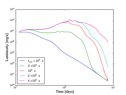
For sufficiently low cutoff times, the effect of the pulsar luminosity becomes small relative to the r-process heating. Notably, in Fig. 2 the light curve for the lowest cutoff time appears to be monotonically decreasing. This is an effect of the fast expansion speed, low mass, low opacity and choice of morphology. In particular, for this morphology the time of peak bolometric luminosity follows (Wollaeger et al., 2018)

$$t_{\rm peak}\approx\\ \left(1\text{ day}\right)\left(\frac{\kappa}{10\text{ cm}^{2}/\text{g}}\right)^{0.35}\left(\frac{M_{\rm ej}}{10^{-2}\text{ M}_{\odot}}\right)^{0.318}\left(\frac{v_{\max}}{0.2c}\right)^{-0.6}\;\;.$$ (13)

Equation (13) gives $t_{\rm peak}\approx 0.05$ day, assuming $\kappa=0.1$ cm²/g. Alternatively, using the scaling relation for time of peak bolometric luminosity from Grossman et al. (2014), $t_{\rm peak}\approx 0.09$ day. The earlier peak time relative to the models of Grossman et al. (2014) is due to the thermal energy contribution to the light curve (Wollaeger et al., 2018).

3.1.2 Magnetic Field Strength Variations and Ejecta Mass and Composition

With a better understanding of the role of the cutoff time, we can now study the dependence of the pulsar-powered light curves on the magnetic field strength for a range of ejecta masses and two different compositions using just two cutoff times: $2\times 10^{4}$, $2\times 10^{5}$ s. We vary the composition by adding a small mass fraction of Nd. Apart from the ejecta mass, magnetic field strength, and composition, the model parameters are the same as in Section 3.1.1. The model parameters are listed in Table 2.

Table 2Parameters for test of mass and magnetic field strength variation.

$t_{\rm cut}$	$\{0.2,2\}\times 10^{5}$ s
$M_{\rm ej}$	$\{1,3,10\}\times 10^{-3}$ M⊙
$v_{\max}/2$	$0.3\,c$
$R$	$1.2\times 10^{6}$ cm
$I$	$1.5\times 10^{45}$ g cm2
$\Omega_{0}$	$2\pi\times 10^{3}$ s-1
$B$	$\{1,10,100\}\times 10^{12}$ G
$\epsilon$	$0.0035$
$\eta$	$1$
$(\chi_{\rm Fe},\chi_{\rm Nd})$	$\{(1,0)\,,\,(1-10^{-4},10^{-4})\}$

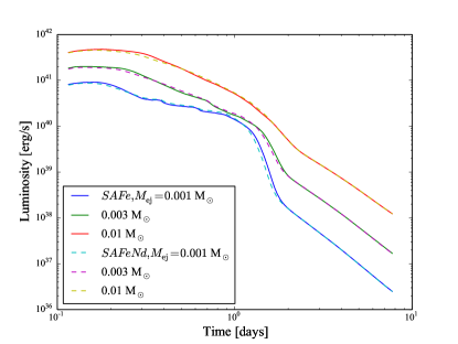
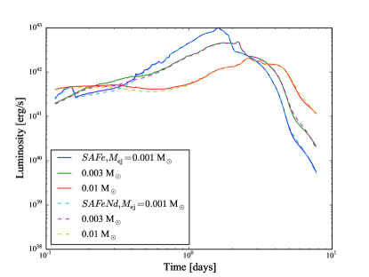
The parameters for the pulsar again imply $t_{\rm gw}=495$ s; the pulsar luminosity is $L_{0}\in\{2.88,288,28800\}\times 10^{43}$ erg/s. Tables 3 and 4 display the luminosity at day 1 for the SAFe models with $2\times 10^{4}$ and $2\times 10^{5}$ s, respectively. Tables 5 and 6 show the same data for the SAFeNd models. For the lowest magnetic field strength, $10^{12}$ G, and lowest remnant cutoff time, increasing the mass produces an upward trend in the luminosity at day 1. For these parameters, the r-process decay energy competes with the pulsar luminosity in setting the kilonova bolometric luminosity at day 1. This is discernible in Fig. 3a, where increasing the ejecta mass can be seen to mask the pulsar peak around day 1. With a remnant lifetime of $2\times 10^{5}$ s, increasing the ejecta mass from 0.001 to 0.003 M_⊙ lowers the luminosity at day 1. The diminished luminosity at day 1 indicates delay in the emission from increased optical depth. For the higher magnetic field strengths, the luminosity at day 1 only decreases when more mass is added, resulting from the increased optical depth. The dimming and delaying of the peak luminosity for the models with $B=10^{13}$ G and $t_{\rm cut}=2\times 10^{5}$ s can be seen in Fig. 3c.

The introduction of the Nd mass fraction, $\chi_{\rm Nd}=10^{-4}$, does not appear to significantly impact the bolometric luminosity, with respect to the pure Fe models. At sufficiently late time, the bolometric luminosity is set by the r-process decay rate. However, the spectrum at later times tends to be redder; in particular for the low-pulsar luminosity, low-remnant time cutoff spectrum shown in Fig. 3c, the spectral features corresponding to the blue transient are systematically dimmer with $\chi_{\rm Nd}=10^{-4}$. In Fig. 3d, the brighter, longer duration pulsar luminosity appears to sustain the blue portion of the spectrum further in time.

Table 3SAFe luminosity (erg/s) at day 1 with $t_{\rm cut}=2\times 10^{4}$ s.

	$10^{12}$	$10^{13}$	$10^{14}$
0.001	$1.41\times 10^{40}$	$7.13\times 10^{41}$	$3.11\times 10^{43}$
0.003	$1.74\times 10^{40}$	$2.60\times 10^{41}$	$4.65\times 10^{42}$
0.01	$5.17\times 10^{40}$	$1.40\times 10^{41}$	$1.93\times 10^{42}$

Table 4SAFe luminosity (erg/s) at day 1 with $t_{\rm cut}=2\times 10^{5}$ s.

	$10^{12}$	$10^{13}$	$10^{14}$
0.001	$9.96\times 10^{40}$	$4.55\times 10^{42}$	$8.52\times 10^{43}$
0.003	$6.48\times 10^{40}$	$2.34\times 10^{42}$	$3.67\times 10^{43}$
0.01	$8.48\times 10^{40}$	$5.36\times 10^{41}$	$1.91\times 10^{43}$

Table 5SAFeNd luminosity (erg/s) at day 1 with $t_{\rm cut}=2\times 10^{4}$ s.

	$10^{12}$	$10^{13}$	$10^{14}$
0.001	$1.49\times 10^{40}$	$7.02\times 10^{41}$	$3.10\times 10^{43}$
0.003	$1.88\times 10^{40}$	$2.65\times 10^{41}$	$4.52\times 10^{42}$
0.01	$5.37\times 10^{40}$	$1.39\times 10^{41}$	$1.76\times 10^{42}$

Table 6SAFeNd luminosity (erg/s) at day 1 with $t_{\rm cut}=2\times 10^{5}$ s.

	$10^{12}$	$10^{13}$	$10^{14}$
0.001	$1.00\times 10^{41}$	$4.52\times 10^{42}$	$8.38\times 10^{43}$
0.003	$6.86\times 10^{40}$	$2.31\times 10^{42}$	$3.63\times 10^{43}$
0.01	$8.57\times 10^{40}$	$5.10\times 10^{41}$	$1.81\times 10^{43}$

(a)

(b)

(c)

(d)

Figure 3.— In Fig. 3a, bolometric luminosity versus time for each mass, for $B=10^{12}$ G and $t_{\rm cut}=2\times 10^{4}$ s. In Fig. 3c, corresponding spectra at day 5.45. The models with mass fraction $\chi_{\rm Nd}=10^{-4}$ have redder emission, despite having similar bolometric luminosity; the blue features corresponding to Fe diminish more quickly after about 2 days. In Fig. 3b, bolometric luminosity versus time for each mass, for $B=10^{13}$ G and $t_{\rm cut}=2\times 10^{5}$ s. In Fig. 3d, corresponding spectra at day 5.45. The persistent, brighter pulsar luminosity model seems to support the blue features of the spectrum persisting longer.

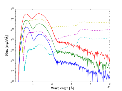
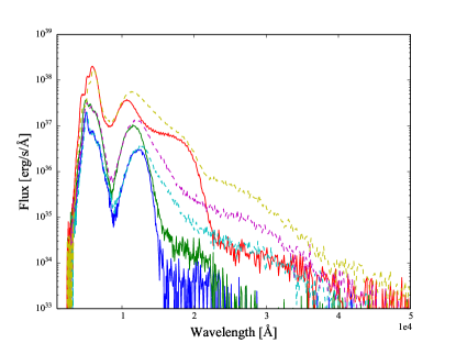
We have tabulated the day 1 and day 7 bolometric luminosities and UBVRIJHK broadband magnitudes for these models in Tables 10-13 of the Appendix. The intent of tabulating the data at early and later time is to identify the effect of variations in the model on evolution of the luminosity and magnitudes. As an example, we can see that the sensitivity of the day 7 model data to remnant cutoff time depends on the pulsar magnetic strength. For instance, in Table 12, for $B=10^{12}$ G and $M_{\rm ej}=0.001$ M_⊙, the B-band magnitude is 32.9 at day 7 for models with either $t_{\rm cut}=2\times 10^{4}$ or $2\times 10^{5}$ s. The same models with $B=10^{13}$ G have day 7 B-band magnitudes of 32.9 and 25.3 for $t_{\rm cut}=2\times 10^{4}$ and $2\times 10^{5}$ s, respectively.

3.1.3 2-component, 2-dimensional Pulsar Results

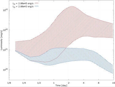
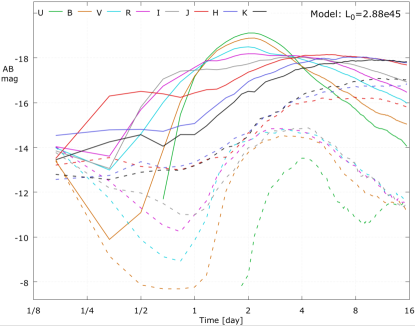
The morphology of the dynamical ejecta of the 2D models is “model A” used by Wollaeger et al. (2018). The wind superimposed on the model A ejecta has the properties described in Section 3.1.1 for $B=10^{12}$ and $10^{13}$ G, but without a remnant cutoff time. These field strengths correspond to initial pulsar luminosities of $2.88\times 10^{43}$ and $2.88\times 10^{45}$ erg/s, respectively. Figure 4 has bolometric luminosity for the range of angular views as shaded regions for each model. These luminosities are “isotropic equivalents”, where each is divided by the solid angle per view and multiplied by 4$\pi$. The angular views are divided into 54 polar angular viewing ranges of equal solid angle. The dimmest light curves (or lowest edge of the shaded regions) correspond to views most closely aligned with the merger plane (“edge-on”), which are most obscured by Nd in the dynamical ejecta. The axial view is over an order of magnitude brighter than for the edge-on view for the model with $B=10^{13}$ G.

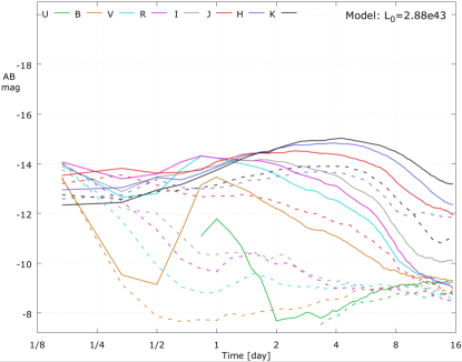
Strong viewing angle dependence is also seen in broadband magnitudes. Figure 5 has plots of UBVRIJHK absolute magnitudes for each model. The viewing angle dependence is stronger for bluer bands, as expected. Before 2 days, the side view (dashed) is not sensitive to the strength of the pulsar luminosity.

Figure 4.— Isotropically equivalent bolometric luminosity versus time for the 2D pulsar kilonova models described in Fig. 1 and Section 3.1.3. The shaded regions represent the range of luminosities from the 54 angular bins that are uniform in the cosine of the polar viewing angle. Brighter luminosity corresponds to viewing bins that are more aligned with the merger axis.

(a)

(b)

Figure 5.— Top (solid) and side (dashed) angular views of the UBVRIJHK magnitudes for the 2D kilonova model described in Fig. 1 and Section 3.1.3. In Fig. 5a, the pulsar source luminosity is $2.88\times 10^{43}$ erg/s. In Fig. 5b, the pulsar source luminosity is $2.88\times 10^{45}$ erg/s.

3.2. Fallback Powered Light Curves

Our fallback models include a range of accretion rates, $\dot{M}$ and ejecta masses. The variations in $\dot{M}$ bound the typical value adopted by Li et al. (2018). These variations in $M_{\rm ej}$ and $\dot{M}$ demonstrate the competition between optical depth and remnant source power, similar to the pulsar variations. Following Section 3.1, we include both 1- and 2-dimensional geometries.

3.2.1 1-dimensional models, Accretion Rates and Ejecta Masses

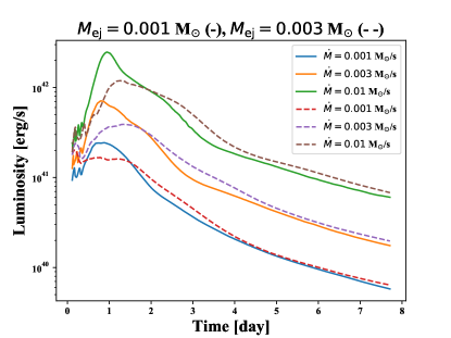
For the 1D fallback models, we vary $v_{\max}$, $\dot{M}$ and $M_{\rm ej}$; otherwise the model parameters of Li et al. (2018) for the fallback luminosity source are adopted, as shown in Eq. (8). The ejecta masses, velocity, and composition are the same here as in Section 3.1.2, permitting direct comparison between these fallback models and a subset of the pulsar models. The model parameters are given in Table 7

Table 7Parameters for test of mass and accretion rate variation.

$L_{0}$	$2\times 10^{51}$ erg/s
$t_{\rm acc}$	0.1 s
$M_{\rm ej}$	$\{1,3,10\}\times 10^{-3}$ M⊙
$v_{\max}/2$	$\{0.3,0.45\}\,c$
$\eta$	$0.1$
$\dot{M}$	$\{1,3,10\}\times 10^{-3}$ M⊙/s
$(\chi_{\rm Fe},\chi_{\rm Nd})$	$(1-10^{-4},10^{-4})$

Figure 6 displays bolometric luminosity versus time for the different accretion rates. Increasing the ejecta mass acts to dim the light curve, since the fallback source is more obscured at higher optical depth. This indicates that much of the kilonova luminosity in these models is derived from radiated accretion energy.

(a)

Figure 6.— Bolometric luminosity versus time for the fallback kilonova model described in Section 3.2.1. The light curves were obtained under the assumption of an ejecta mass of 0.001 M_⊙ (solid) or 0.003 M_⊙ (dashed) and the three accretion rates.

In the Appendix, UBVRIJHK band data at day 1 and day 7 are provided for these fallback models in Tables 14–15. The accretion rate impacts the rate of decline in the optical bands. For instance, for $M_{\rm ej}=0.001$ M_⊙ and $v_{\max}/2=0.3c$, accretion rates of $\dot{M}=0.001$, $\dot{M}=0.003$, and $\dot{M}=0.01$ M_⊙/s drop by $\sim$4.2, 3.5, and 2.8 magnitudes in the V-band, respectively. Likewise, the R-band drops by $\sim$3.9, 3.2, and 2.7 magnitudes, respectively. The J through K-bands are relatively insensitive to the fallback source at day 1, but their brightness is more affected by day 7, where the variation with accretion rate is $>1$ magnitude. In other words, at early time, the JKH magnitudes appear to be mainly set by $M_{\rm ej}$, while at later time, there is a systematic increase in magnitude with increasing accretion rate. For the high-velocity models, day 1 is later in the evolution of the light curves, so these trends are not reflected in the broadband data.

3.2.2 2-component, 2-dimensional Accretion Results

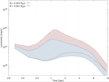
For the fallback models in 2D, we again use the “model A” morphology, as in Section 3.1.3. The wind superimposed on the model A ejecta has the properties described in Section 3.2.1 for $\dot{M}=0.001$ and 0.003 M_⊙/s, and with a wind mass of 0.001 M_⊙. Figure 7 has bolometric luminosity for the range of angular views as shaded regions for each model. As in Fig. 4, the values are shown as isotropic equivalents. The angular views are again divided into 54 polar angular viewing ranges of equal solid angle, with edge-on views being dimmest. Relative to the 2D pulsar models, the variation with respect to viewing angle does not change as substantially when increasing the source luminosity. This is partly explained by the fallback luminosity scaling linearly with accretion rate, whereas the pulsar source luminosity scales as the square of the magnetic field strength. As in the 2D pulsar models, increasing the remnant source luminosity affects the rise and decline times for near-on-axis angular views of the ejecta.

Figure 7.— Isotropically equivalent bolometric luminosity versus time for the 2D fallback kilonova models described in Fig. 1 and Section 3.2.2. The shaded regions represent the range of luminosities from the 54 angular bins that are uniform in the cosine of the polar viewing angle. Brighter luminosity corresponds to viewing bins that are more aligned with the merger axis.

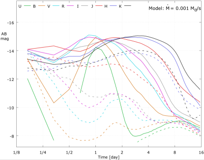
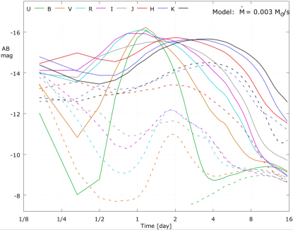
Strong viewing angle dependence is again seen in broadband magnitudes. Figure 8 has plots of UBVRIJHK absolute magnitudes for each model. The viewing angle dependence is stronger for bluer bands, as expected. Before 2 days, the side view (dashed) is not sensitive to the strength of the pulsar luminosity. Unlike the 2D pulsar models, the U-band does not significantly shift in time and peak brightness when going to a higher remnant source, which is due to the more modest increase in luminosity relative to the pulsar models.

(a)

(b)

Figure 8.— Top (solid) and side (dashed) angular views of the UBVRIJHK magnitudes for the 2D kilonova model described in Fig. 1 and Section 3.2.2. In Fig. 8a, the fallback accretion rate is 0.001 M_⊙/s. In Fig. 8b, the fallback accretion rate is 0.003 M_⊙/s.

3.3. Accretion versus Pulsar Power

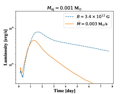
With our two simple prescriptions for accretion and pulsar power sources, we produce different light curves. In Figure 9, we compare a fallback model with $\dot{M}=0.003$ M_⊙/s to a pulsar model with $B=3.4\times 10^{12}$ G. It is evident that the slope of the light-curve tails are eventually set by the time-dependence of the remnant source.

(a)

Figure 9.— Bolometric luminosity versus time comparing the fallback energy source to the pulsar energy source. The figure compares a fallback model with a $\dot{M}=0.003$ M_⊙/s to a pulsar model with $B=3.4\times 10^{12}$ G. The slopes of the light-curve tails are eventually set by the time-dependence of the remnant source.

3.3.1 AT 2017gfo

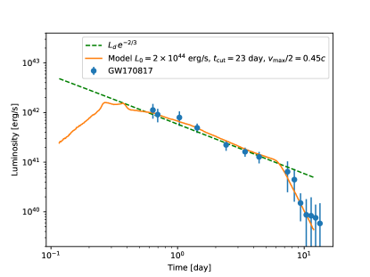
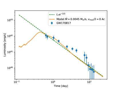
We can compare our two different additional power sources to observations of AT 2017gfo using the results of Li et al. (2018) and Piro et al. (2018) as a starting point. Although there is a qualitative agreement with those results, there are some differences in our conclusions. For the polar ejecta mass of 0.001 M_⊙ given by Li et al. (2018), our ejecta model requires a slightly lower pulsar luminosity and somewhat higher wind outflow speed than previously published: $2\times 10^{44}$ instead of $3.4\times 10^{44}$ erg/s and $0.45c$ instead of $0.35c$. Additionally, we find that this model fits the later time bolometric luminosity better with a remnant cutoff time of about $\sim 10$ observer days. From the modeling perspective, some differences here include the use of multifrequency opacity tables and a detailed high-latitude r-process heating rate (corresponding to the “Wind 1” composition of Wollaeger et al. (2018)) derived from WinNet (Winteler, 2012; Winteler et al., 2012). For the fallback model, similar to the polar model of Li et al. (2018), we find an accretion rate of 0.003-0.0045 M_⊙/s gives bolometric luminosity in the range of the observation, but with a velocity of $\sim 0.4c$ instead of $0.25c$. Parameters for the pulsar and fallback models are given in Tables and, respectively.

Table 8Parameters for pulsar fit of AT 2017gfo.

$M_{\rm ej}$	$10^{-3}$ M⊙
$v_{\max}/2$	$0.45\,c$
$L_{0}$	$2\times 10^{44}$ erg/s
$t_{\rm gw}$	495 s
$t_{\rm cut}$	$2\times 10^{6}$ s
$(\chi_{\rm Fe},\chi_{\rm Nd})$	$(1-10^{-3},10^{-3})$

Table 9Parameters for fallback fit of AT 2017gfo.

$M_{\rm ej}$	$10^{-3}$ M⊙
$v_{\max}/2$	$0.4\,c$
$L_{0}$	$2\times 10^{51}$ erg/s
$\eta$	$0.1$
$\dot{M}$	$4.5\times 10^{-3}$ M⊙/s
$t_{\rm acc}$	0.1 s
$(\chi_{\rm Fe},\chi_{\rm Nd})$	$(1-10^{-3},10^{-3})$

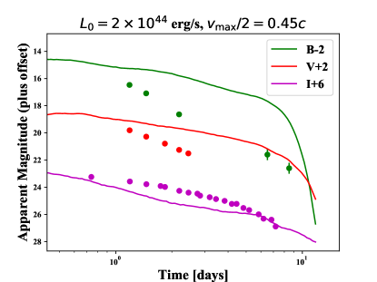
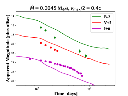
Figure 10 has bolometric and broadband luminosity versus time for our attempt to match AT 2017gfo with a pulsar and a fallback model. Despite the decent agreement in bolometric luminosity in Fig. 10a, it is apparent in 10b that this model produces blue emission that does not decay quickly enough with respect to the observation. Figure 10c has the light curve for the fallback model. The fallback model bolometric luminosity does not fit the data as well at intermediate times, implying the decline in the source luminosity is too rapid to fully account for this emission, as found by Li et al. (2018). However, the trends in the B and V bands are much more similar to those of AT 2017gfo, relative to the pulsar model. The I-band of the fallback model is not bright enough at later times, which may be part of the disk.

(a) Pulsar

(b) Pulsar

(c) Fallback

(d) Fallback

Figure 10.— In Figs. 10a and 10c, bolometric luminosity versus time of the pulsar and fallback source models, respectively, described in Section 3.3.1, along with AT 2017gfo luminosity data from Piro et al. (2018). Overplotted are the remnant source luminosities (dashed green), Eqs. (3) and (8) multiplied by an attenuation factor, $e^{-2/3}\approx 0.5$. In Figs. 10b and 10d, B, V, and I broadband magnitude versus time for the pulsar and fallback source models in Section 3.3.1 along with broadband data from Troja et al. (2017). The trends in the B and V-bands of the observed data are better fit by the fallback model, which has a source luminosity that declines more rapidly (Eq. (8)). Figures 10a and 10b are derived from the spectra of the model presented in Table 8, and Figs. 10c and 10d are from the spectra of the model presented in Table 9.

4. Conclusions

We have explored several models of remnant source energy contributions to the kilonova optical/IR signal. These models are to serve as part of a larger database of models to which future observed kilonovae can be compared. Below we summarize our findings for this subset of models.

• Our attempt to fit AT 2017gfo in both bolometric luminosity and broadband light curves is unsuccessful. For a pulsar model fit of the bolometric luminosity, the broadband data is too blue in our tests, despite having an I-band in reasonable agreement with the observation. On the other hand, for the fallback model fit, the B and V-bands appear to be more consistent, but the I-band declines too rapidly. Moreover, the trend in the bolometric luminosity of the fallback model does not appear to fit well from a few days to a week. However, we stress that our attempt to fit AT 2017gfo is not an exhaustive study, and that caution must be taken when attempting to draw conclusions from the fits. In particular, while the calculations were multi-frequency, we only tested with Fe and Nd. Expanding the set of elements in these models could affect the trends in the broadband magnitudes.

• For the grid of models in which the remnant cutoff time, $t_{\rm cut}$, was varied, we find that, for a pulsar luminosity comparable to that of Li et al. (2018), $t_{\rm cut}\gtrsim$ 1 day saturates the peak luminosity. The velocity of $\sim 0.3c$ evidently permits the effective photosphere to recede quickly enough that the pulsar energy can be uncovered on a $\gtrsim 1$ day timescale.

• As expected, increasing the pulsar luminosity and lifetime generally increases the brightness of these models. Increasing ejecta mass may either increase or decrease the kilonova luminosity. In particular, going from $0.001$ to $0.01$ M_⊙ increases the r-process heating enough to mask the contribution of the low pulsar luminosity ($\sim 10^{43}$ erg/s) to the kilonova luminosity at 1 day. In contrast, with high pulsar luminosity, making the same increases to the ejecta mass lowers the luminosity at 1 day. This behavior is due to the optical depth increasing while the total r-process heating remains sub-dominant with respect to the pulsar luminosity.

• With a small contribution of Nd, the H and K bands remain brighter at day 7 for models with ejecta mass $\geq 0.003$ M_⊙ and magnetic field $\geq 10^{13}$ G, despite these models having similar broadband luminosity at day 1 to the versions with pure Fe.

• Following Metzger (2017); Li et al. (2018), the luminosity from fallback can significantly impact the luminosity of the kilonova model. As expected, the decay of the kilonova bolometric light-curve tail is set by the time-dependence of the remnant source. For similar source luminosity, the spectra from the fallback models are similar to those of the pulsar models; it is primarily a function of the ejecta composition. The slower decline of the luminosity tails of the pulsar models permit them to stay more luminous and have bluer spectra at later time.

• The 2D models show that the remnant source luminosity can affect viewing-angle dependence of the light curves. In particular, at early time (for instance, $\lesssim 1/2$ day for the pulsar models explored), edge-on (off-axis) views of the ejecta produce broadband and bolometric light curves that are insensitive to the brightness of the pulsar source. As the photosphere recedes through the dynamical ejecta, the remnant source begins to contribute to the observable light curve. After 1/2 day, the time of peak magnitude for the U and B bands is shifted earlier by a few days in the higher-source energy model, while the edge on views for these bands are substantially re-brightened after the initial time.

Future work will involve attempting to refine the parameters, identifying model deficiencies, and comparing to new observations during the LIGO O3 run. The models presented in this work are a first step towards these efforts. Some concepts we have gleaned from the remnant source study, that may be useful to further modeling efforts to match AT 2017gfo, are (1) the dependence of bolometric luminosity and broadband magnitudes on the time dependence of the remnant source, and (2) the competition between r-process decay heating, the remnant source luminosity, and optical depth for certain model parameters.

Appendix A Luminosity & Broadband Magnitudes for Pulsar Kilonova Models

Table 10Luminosity (erg/s) and 40 Mpc UBVRIJHK bands at day 1 of SAFe model from Section 3.1.2.

$t_{\rm cut}$ (s), $B$ (G), $M_{\rm ej}$ (M⊙)	$L_{\rm bol}$	U	B	V	R	I	J	H	K
$2\times 10^{4}$, $10^{12}$, 0.001	$1.41\times 10^{40}$	30.1	27.0	23.3	21.6	21.6	19.7	20.0	23.4
0.003	$1.74\times 10^{40}$	29.4	26.5	23.8	21.4	21.0	19.7	19.8	21.5
0.01	$5.17\times 10^{40}$	28.1	25.3	22.9	20.5	19.8	18.9	18.5	19.3
$10^{13}$, 0.001	$7.13\times 10^{41}$	17.0	16.8	16.5	17.0	18.2	18.8	19.1	21.7
0.003	$2.60\times 10^{41}$	24.7	21.9	17.8	17.1	17.7	17.8	18.4	20.1
0.01	$1.40\times 10^{41}$	27.7	24.6	21.0	18.4	18.0	17.8	17.9	18.9
$10^{14}$, 0.001	$3.11\times 10^{43}$	13.1	14.0	12.5	11.9	13.7	15.2	17.1	17.8
0.003	$4.65\times 10^{42}$	19.5	17.2	14.8	14.0	14.7	14.6	16.0	16.7
0.01	$1.93\times 10^{42}$	22.2	19.8	17.0	16.2	16.7	14.7	15.1	15.8
$2\times 10^{5}$, $10^{12}$, 0.001	$9.96\times 10^{40}$	22.7	20.2	18.2	18.4	20.2	19.1	19.5	23.3
0.003	$6.48\times 10^{40}$	28.4	25.8	20.5	18.8	19.1	18.9	19.2	21.1
0.01	$8.48\times 10^{40}$	27.6	25.0	22.0	19.2	18.6	18.5	18.3	19.1
$10^{13}$, 0.001	$4.55\times 10^{42}$	15.1	15.6	14.6	14.1	15.8	17.4	18.9	19.9
0.003	$2.34\times 10^{42}$	17.4	16.6	15.2	14.9	15.5	16.4	17.7	18.8
0.01	$5.36\times 10^{41}$	24.4	21.9	17.9	16.9	17.0	16.1	16.8	17.7
$10^{14}$, 0.001	$8.52\times 10^{43}$	12.5	13.5	11.6	10.8	11.5	12.7	14.5	15.3
0.003	$3.67\times 10^{43}$	15.8	15.6	13.1	12.1	12.2	12.1	13.5	14.2
0.01	$1.91\times 10^{43}$	19.2	17.2	15.6	14.6	14.1	12.2	12.6	13.2

Table 11Luminosity (erg/s) and 40 Mpc UBVRIJHK bands at day 1 of SAFeNd model from Section 3.1.2.

$t_{\rm cut}$ (s), $B$ (G), $M_{\rm ej}$ (M⊙)	$L_{\rm bol}$	U	B	V	R	I	J	H	K
$2\times 10^{4}$, $10^{12}$, 0.001	$1.49\times 10^{40}$	30.6	27.4	23.9	21.8	21.5	19.6	20.0	22.2
0.003	$1.88\times 10^{40}$	29.6	26.7	23.9	21.4	21.0	19.6	19.7	21.0
0.01	$5.37\times 10^{40}$	28.3	25.5	22.9	20.6	19.8	18.8	18.5	19.0
$10^{13}$, 0.001	$7.02\times 10^{41}$	17.1	16.8	16.5	17.0	18.1	18.3	19.0	21.1
0.003	$2.65\times 10^{41}$	24.9	22.1	17.9	17.1	17.7	17.6	18.4	19.7
0.01	$1.39\times 10^{41}$	27.7	24.6	21.0	18.5	18.1	17.8	18.0	18.6
$10^{14}$, 0.001	$3.10\times 10^{43}$	13.2	14.0	12.6	11.9	13.7	15.2	16.9	17.9
0.003	$4.52\times 10^{42}$	19.2	17.1	14.8	14.1	14.8	14.6	16.0	16.8
0.01	$1.76\times 10^{42}$	22.5	19.8	16.9	16.2	16.8	14.6	15.2	15.8
$2\times 10^{5}$, $10^{12}$, 0.001	$1.00\times 10^{41}$	23.5	20.7	18.4	18.4	20.0	18.6	19.4	21.6
0.003	$6.86\times 10^{40}$	28.6	25.9	20.7	18.8	19.1	18.6	19.1	20.5
0.01	$8.57\times 10^{40}$	27.9	25.1	22.0	19.3	18.7	18.4	18.3	18.9
$10^{13}$, 0.001	$4.52\times 10^{42}$	15.1	15.6	14.6	14.1	15.8	17.3	18.7	19.7
0.003	$2.31\times 10^{42}$	17.5	16.6	15.2	14.9	15.5	16.2	17.5	18.7
0.01	$5.10\times 10^{41}$	25.2	22.5	18.1	16.9	17.1	16.1	16.9	17.6
$10^{14}$, 0.001	$8.38\times 10^{43}$	12.5	13.5	11.6	10.8	11.5	12.7	14.4	15.3
0.003	$3.63\times 10^{43}$	15.5	15.4	13.1	12.4	12.3	12.1	13.5	14.1
0.01	$1.81\times 10^{43}$	18.5	16.6	15.4	14.6	14.3	12.2	12.6	13.2

Table 12Luminosity (erg/s) and 40 Mpc UBVRIJHK bands at day 7 of SAFe model from Section 3.1.2.

$t_{\rm cut}$ (s), $B$ (G), $M_{\rm ej}$ (M⊙)	$L_{\rm bol}$	U	B	V	R	I	J	H	K
$2\times 10^{4}$, $10^{12}$, 0.001	$3.42\times 10^{36}$	35.9	32.9	30.3	29.4	29.3	31.1	30.6	35.1
0.003	$2.29\times 10^{37}$	34.3	30.9	28.4	27.6	27.5	27.8	27.7	31.8
0.01	$1.63\times 10^{38}$	32.8	29.0	26.7	25.9	25.8	25.0	25.1	28.9
$10^{13}$, 0.001	$4.82\times 10^{36}$	35.9	32.9	30.3	29.4	29.1	30.7	29.4	30.0
0.003	$2.84\times 10^{37}$	34.3	30.9	28.4	27.6	27.5	27.6	27.3	28.2
0.01	$1.78\times 10^{38}$	32.8	29.0	26.7	25.9	25.8	25.0	24.9	27.5
$10^{14}$, 0.001	$4.05\times 10^{40}$	23.4	20.1	19.5	19.9	21.3	19.5	25.4	25.8
0.003	$2.81\times 10^{41}$	20.9	17.9	17.1	17.4	18.8	19.9	23.8	26.2
0.01	$1.37\times 10^{42}$	19.1	16.1	15.4	15.7	17.9	19.7	22.1	22.3
$2\times 10^{5}$, $10^{12}$, 0.001	$3.44\times 10^{36}$	35.9	32.9	30.3	29.4	29.3	31.1	30.6	34.2
0.003	$2.29\times 10^{37}$	34.3	30.9	28.4	27.6	27.5	27.8	27.7	31.6
0.01	$1.63\times 10^{38}$	32.8	29.0	26.7	25.9	25.8	25.0	25.1	28.9
$10^{13}$, 0.001	$1.06\times 10^{40}$	30.9	25.3	21.9	20.7	21.0	21.7	20.2	26.7
0.003	$3.55\times 10^{40}$	28.6	24.3	21.1	19.8	19.9	19.4	19.0	24.2
0.01	$1.63\times 10^{41}$	26.8	22.7	20.0	18.6	18.8	17.0	17.8	20.0
$10^{14}$, 0.001	$4.53\times 10^{42}$	15.5	16.4	17.7	19.7	21.9	26.5	33.5	75.7
0.003	$1.01\times 10^{43}$	14.5	15.2	17.8	18.9	20.4	25.5	26.5	31.8
0.01	$2.16\times 10^{43}$	13.3	14.3	15.3	15.9	17.3	21.9	22.8	27.0

Table 13Luminosity (erg/s) and 40 Mpc UBVRIJHK bands at day 7 of SAFeNd model from Section 3.1.2.

$t_{\rm cut}$ (s), $B$ (G), $M_{\rm ej}$ (M⊙)	$L_{\rm bol}$	U	B	V	R	I	J	H	K
$2\times 10^{4}$, $10^{12}$, 0.001	$3.40\times 10^{36}$	-	-	44.0	40.5	38.3	34.7	34.4	33.8
0.003	$2.27\times 10^{37}$	131.9	46.8	38.3	34.6	32.7	30.4	30.5	30.6
0.01	$1.63\times 10^{38}$	86.4	38.3	33.2	30.3	28.6	26.8	27.2	27.5
$10^{13}$, 0.001	$4.54\times 10^{36}$	145.7	60.4	43.9	39.0	36.4	32.2	31.8	29.9
0.003	$2.58\times 10^{37}$	-	47.3	38.1	34.4	32.0	29.7	29.3	29.4
0.01	$1.80\times 10^{38}$	-	38.1	33.2	30.2	28.3	26.6	26.2	27.1
$10^{14}$, 0.001	$4.56\times 10^{40}$	23.5	20.2	19.3	19.8	21.1	19.2	20.7	22.2
0.003	$2.93\times 10^{41}$	21.4	18.2	17.2	17.5	18.7	18.0	19.2	20.8
0.01	$1.39\times 10^{42}$	19.7	16.4	15.5	15.7	17.7	16.5	17.8	19.1
$2\times 10^{5}$, $10^{12}$, 0.001	$3.44\times 10^{36}$	137.7	50.9	44.5	40.7	38.5	34.7	34.3	33.8
0.003	$2.27\times 10^{37}$	132.0	45.9	38.2	34.6	32.8	30.4	30.5	30.6
0.01	$1.63\times 10^{38}$	89.3	38.3	33.3	30.3	28.6	26.8	27.2	27.6
$10^{13}$, 0.001	$1.02\times 10^{40}$	31.3	25.7	22.2	20.8	21.1	21.8	20.1	23.7
0.003	$3.53\times 10^{40}$	29.7	24.9	21.5	20.0	19.8	19.6	18.7	22.1
0.01	$1.74\times 10^{41}$	28.7	23.8	20.8	19.0	18.5	17.1	17.2	19.5
$10^{14}$, 0.001	$4.59\times 10^{42}$	15.5	16.4	17.5	18.9	19.7	18.6	20.8	21.7
0.003	$1.00\times 10^{43}$	14.5	15.2	17.3	18.3	18.2	18.8	20.0	20.9
0.01	$2.21\times 10^{43}$	13.3	14.2	15.1	15.7	16.4	17.4	17.9	19.9

Appendix B Luminosity & Broadband Magnitudes for Fallback Kilonova Models

Table 14Luminosity (erg/s) and 40 Mpc UBVRIJHK bands at day 1 of SAFeNd model with fallback source, from Section 3.2.1.

$v_{\max}/2$ ($c$), $M_{\rm ej}$ (M⊙), $\dot{M}$ (M⊙/s)	$L_{\rm bol}$	U	B	V	R	I	J	H	K
0.3, 0.001, 0.001	$1.34\times 10^{41}$	20.0	18.2	17.4	17.9	19.4	18.7	19.1	21.2
, 0.003	$3.88\times 10^{41}$	17.4	16.9	16.8	17.5	19.1	19.2	19.5	21.1
, 0.01	$9.72\times 10^{41}$	15.8	15.9	16.1	16.6	17.8	18.9	19.7	21.0
, 0.003, 0.001	$2.56\times 10^{40}$	24.8	22.4	18.3	17.8	19.0	17.9	18.5	20.2
, 0.003	$5.75\times 10^{40}$	21.3	19.0	16.8	17.1	18.2	17.6	18.4	20.1
, 0.01	$2.53\times 10^{41}$	18.0	16.8	16.0	16.4	17.1	17.2	18.1	19.6
, 0.01, 0.001	$5.14\times 10^{40}$	27.4	24.8	20.0	18.2	18.4	17.9	18.2	18.8
, 0.003	$5.18\times 10^{40}$	26.6	23.8	18.2	17.2	17.9	17.3	17.9	18.7
, 0.01	$6.18\times 10^{40}$	25.2	21.7	17.1	16.6	17.5	16.8	17.5	18.4
0.45, 0.001, 0.001	$9.62\times 10^{40}$	23.7	19.4	18.8	19.1	20.0	18.6	19.0	20.2
, 0.003	$2.72\times 10^{41}$	19.8	17.6	17.6	18.2	18.9	18.4	19.1	20.4
, 0.01	$8.55\times 10^{41}$	16.6	16.5	16.7	17.4	18.5	18.4	19.1	20.4
, 0.003, 0.001	$1.07\times 10^{41}$	25.8	20.8	19.1	19.1	19.6	17.9	18.0	20.5
, 0.003	$3.18\times 10^{41}$	22.4	18.5	17.5	17.8	18.8	17.2	17.6	18.6
, 0.01	$1.09\times 10^{42}$	18.1	16.3	16.0	16.5	17.5	17.0	17.8	18.8
, 0.01, 0.001	$1.32\times 10^{41}$	30.0	25.0	20.8	19.5	19.3	17.2	17.5	20.2
, 0.003	$4.14\times 10^{41}$	26.2	21.8	18.2	17.6	18.3	16.2	16.6	19.0
, 0.01	$1.44\times 10^{42}$	21.6	17.7	15.6	15.8	17.1	15.6	16.1	17.6

Table 15Luminosity (erg/s) and 40 Mpc UBVRIJHK bands at day 7 of SAFeNd model with fallback source, from Section 3.2.1.

$v_{\max}/2$ ($c$), $M_{\rm ej}$ (M⊙), $\dot{M}$ (M⊙/s)	$L_{\rm bol}$	U	B	V	R	I	J	H	K
0.3, 0.001, 0.001	$7.66\times 10^{39}$	27.2	23.3	21.6	21.8	22.4	20.7	22.2	23.8
, 0.003	$2.44\times 10^{40}$	25.3	21.5	20.3	20.7	21.3	19.9	20.6	23.0
, 0.01	$8.61\times 10^{40}$	22.6	19.4	18.9	19.3	20.5	19.2	20.0	22.1
, 0.003, 0.001	$9.21\times 10^{39}$	31.8	24.4	22.3	21.8	22.2	20.2	22.1	23.3
, 0.003	$3.45\times 10^{40}$	28.4	22.4	20.7	20.6	21.1	19.2	20.3	22.4
, 0.01	$1.14\times 10^{41}$	25.3	20.1	18.9	19.3	19.9	18.3	18.8	21.2
, 0.01, 0.001	$1.80\times 10^{40}$	37.8	27.4	24.5	22.4	22.4	19.9	22.4	22.8
, 0.003	$5.65\times 10^{40}$	32.3	25.3	22.8	21.1	21.1	18.7	20.4	21.8
, 0.01	$1.54\times 10^{41}$	27.6	22.3	20.2	19.6	19.6	17.6	18.2	20.7
0.45, 0.001, 0.001	$3.18\times 10^{39}$	25.5	23.3	22.2	22.9	23.5	22.4	23.5	24.1
, 0.003	$8.60\times 10^{39}$	23.2	22.1	21.5	21.9	22.5	21.5	22.5	23.3
, 0.01	$2.86\times 10^{40}$	21.5	20.7	20.3	20.5	21.3	20.6	21.2	22.5
, 0.003, 0.001	$3.40\times 10^{39}$	29.3	23.6	22.1	22.7	23.3	22.0	23.6	24.1
, 0.003	$8.90\times 10^{39}$	24.8	22.5	21.1	21.8	22.2	20.8	22.3	23.0
, 0.01	$2.63\times 10^{40}$	22.3	21.0	20.2	20.6	21.1	19.9	20.8	22.1
, 0.01, 0.001	$3.14\times 10^{39}$	37.7	24.7	22.8	22.4	23.3	21.6	24.1	24.0
, 0.003	$9.38\times 10^{39}$	28.6	23.0	21.3	21.4	22.1	20.5	22.6	22.9
, 0.01	$2.90\times 10^{40}$	24.9	21.7	20.0	20.4	20.9	19.3	20.9	21.8

References

- Abbott et al. (2017a) Abbott, B. P., et al. 2017a, ApJ, 850, L39
- Abbott et al. (2017b) —. 2017b, ApJ, 848, L13
- Abbott et al. (2017c) —. 2017c, ApJ, 848, L12
- Abdikamalov et al. (2012) Abdikamalov, E., Burrows, A., Ott, C. D., Löffler, F., O’Connor, E., Dolence, J. C., & Schnetter, E. 2012, ApJ, 755, 111
- Alexander et al. (2017) Alexander, K. D., et al. 2017, ApJ, 848, L21
- Andreoni et al. (2017) Andreoni, I., et al. 2017, Publications of the Astronomical Society of Australia, 34, e069
- Arcavi et al. (2017a) Arcavi, I., et al. 2017a, Nature, 551, 64
- Arcavi et al. (2017b) —. 2017b, ApJ, 848, L33
- Bauswein et al. (2013) Bauswein, A., Goriely, S., & Janka, H.-T. 2013, ApJ, 773, 78
- Bloom et al. (1999) Bloom, J. S., Sigurdsson, S., & Pols, O. R. 1999, MNRAS, 305, 763
- Briggs (1993) Briggs, M. S. 1993, ApJ, 407, 126
- Chevalier (1989) Chevalier, R. A. 1989, ApJ, 346, 847
- Chornock et al. (2017) Chornock, R., et al. 2017, ApJ, 848, L19
- Cleveland & Gentile (2014) Cleveland, M. A., & Gentile, N. 2014, Transport Theory and Statistical Physics, 1
- Côté et al. (2018) Côté, B., et al. 2018, ApJ, 855, 99
- Coulter et al. (2017) Coulter, D. A., et al. 2017, Science, 358, 1556
- Cowperthwaite et al. (2017) Cowperthwaite, P. S., et al. 2017, ApJ, 848, L17
- Densmore et al. (2012) Densmore, J. D., Thompson, K. G., & Urbatsch, T. J. 2012, Journal of Computational Physics, 231, 6924
- Díaz et al. (2017) Díaz, M. C., et al. 2017, ApJ, 848, L29
- Drout et al. (2017) Drout, M. R., et al. 2017, Science, 358, 1570
- Evans et al. (2017) Evans, P. A., et al. 2017, Science, 358, 1565
- Fermi-LAT Collaboration (2017) Fermi-LAT Collaboration. 2017, arXiv e-prints, arXiv:1710.05450
- Fong & Berger (2013) Fong, W., & Berger, E. 2013, ApJ, 776, 18
- Fontes et al. (2019) Fontes, C. J., Fryer, C. L., Hungerford, A. L., Wollaeger, R. T., & Korobkin, O. 2019, arXiv e-prints, arXiv:1904.08781
- Fontes et al. (2017) Fontes, C. J., Fryer, C. L., Hungerford, A. L., Wollaeger, R. T., Rosswog, S., & Berger, E. 2017, arXiv e-prints, arXiv:1702.02990
- Fontes et al. (2015) Fontes, C. J., et al. 2015, Journal of Physics B: Atomic, Molecular and Optical Physics, 48, 144014
- Freiburghaus et al. (1999) Freiburghaus, C., Rosswog, S., & Thielemann, F.-K. 1999, ApJ, 525, L121
- Fryer (2009) Fryer, C. L. 2009, ApJ, 699, 409
- Fryer et al. (1999) Fryer, C. L., Woosley, S. E., & Hartmann, D. H. 1999, ApJ, 526, 152
- Fujibayashi et al. (2018) Fujibayashi, S., Kiuchi, K., Nishimura, N., Sekiguchi, Y., & Shibata, M. 2018, ApJ, 860, 64
- Gaigalas et al. (2019) Gaigalas, G., Kato, D., Rynkun, P., Radziute, L., & Tanaka, M. 2019, arXiv e-prints, arXiv:1901.10671
- Goldstein et al. (2017) Goldstein, A., et al. 2017, ApJ, 848, L14
- Grossman et al. (2014) Grossman, D., Korobkin, O., Rosswog, S., & Piran, T. 2014, MNRAS, 439, 757
- Haggard et al. (2017) Haggard, D., Nynka, M., Ruan, J. J., Kalogera, V., Cenko, S. B., Evans, P., & Kennea, J. A. 2017, ApJ, 848, L25
- Hallinan et al. (2017) Hallinan, G., et al. 2017, Science, 358, 1579
- Jackson (1999) Jackson, J. D. 1999, Classical Electrodynamics, 3rd Ed. (John Wiley & Sons, Inc.)
- Kasen et al. (2017) Kasen, D., Metzger, B., Barnes, J., Quataert, E., & Ramirez-Ruiz, E. 2017, Nature, 551, 80
- Kasliwal et al. (2017) Kasliwal, M. M., et al. 2017, Science, 358, 1559
- Kasliwal et al. (2019) —. 2019, MNRAS, L14
- Kawaguchi et al. (2018) Kawaguchi, K., Shibata, M., & Tanaka, M. 2018, ApJ, 865, L21
- Kilpatrick et al. (2017) Kilpatrick, C. D., et al. 2017, Science, 358, 1583
- Kim et al. (2017) Kim, S., et al. 2017, ApJ, 850, L21
- Kisaka et al. (2016) Kisaka, S., Ioka, K., & Nakar, E. 2016, ApJ, 818, 104
- Korobkin et al. (2012) Korobkin, O., Rosswog, S., Arcones, A., & Winteler, C. 2012, MNRAS, 426, 1940
- Kouveliotou et al. (1993) Kouveliotou, C., Meegan, C. A., Fishman, G. J., Bhat, N. P., Briggs, M. S., Koshut, T. M., Paciesas, W. S., & Pendleton, G. N. 1993, ApJ, 413, L101
- Lasky & Glampedakis (2016) Lasky, P. D., & Glampedakis, K. 2016, Monthly Notices of the Royal Astronomical Society, 458, 1660
- Lattimer & Schramm (1974) Lattimer, J. M., & Schramm, D. N. 1974, ApJ, 192, L145
- Li et al. (2018) Li, S.-Z., Liu, L.-D., Yu, Y.-W., & Zhang, B. 2018, ApJ, 861, L12
- Lippuner & Roberts (2015) Lippuner, J., & Roberts, L. F. 2015, ApJ, 815, 82
- Lipunov et al. (2017) Lipunov, V. M., et al. 2017, ApJ, 850, L1
- Matsumoto et al. (2018) Matsumoto, T., Ioka, K., Kisaka, S., & Nakar, E. 2018, ApJ, 861, 55
- McCully et al. (2017) McCully, C., et al. 2017, ApJ, 848, L32
- Metzger (2017) Metzger, B. D. 2017, Living Reviews in Relativity, 20, 3
- Metzger & Fernández (2014) Metzger, B. D., & Fernández, R. 2014, MNRAS, 441, 3444
- Metzger & Piro (2014) Metzger, B. D., & Piro, A. L. 2014, MNRAS, 439, 3916
- Metzger et al. (2018) Metzger, B. D., Thompson, T. A., & Quataert, E. 2018, ApJ, 856, 101
- Mumpower et al. (2016) Mumpower, M. R., Surman, R., McLaughlin, G. C., & Aprahamian, A. 2016, Progress in Particle and Nuclear Physics, 86, 86
- Nicholl et al. (2017) Nicholl, M., et al. 2017, ApJ, 848, L18
- Perego et al. (2014) Perego, A., Rosswog, S., Cabezón, R. M., Korobkin, O., Käppeli, R., Arcones, A., & Liebendörfer, M. 2014, MNRAS, 443, 3134
- Pian et al. (2017) Pian, E., et al. 2017, Nature, 551, 67
- Piro et al. (2018) Piro, L., et al. 2018, MNRAS
- Popham et al. (1999) Popham, R., Woosley, S. E., & Fryer, C. 1999, ApJ, 518, 356
- Radice et al. (2016) Radice, D., Galeazzi, F., Lippuner, J., Roberts, L. F., Ott, C. D., & Rezzolla, L. 2016, MNRAS, 460, 3255
- Radice et al. (2018a) Radice, D., Perego, A., Bernuzzi, S., & Zhang, B. 2018a, MNRAS, 481, 3670
- Radice et al. (2018b) Radice, D., Perego, A., Hotokezaka, K., Bernuzzi, S., Fromm, S. A., & Roberts, L. F. 2018b, ArXiv e-prints
- Rosswog (2013) Rosswog, S. 2013, Philosophical Transactions of the Royal Society of London Series A, 371, 20272
- Rosswog et al. (2014) Rosswog, S., Korobkin, O., Arcones, A., Thielemann, F. K., & Piran, T. 2014, MNRAS, 439, 744
- Rowlinson et al. (2014) Rowlinson, A., Gompertz, B. P., Dainotti, M., O’Brien, P. T., Wijers, R. A. M. J., & van der Horst, A. J. 2014, MNRAS, 443, 1779
- Savchenko et al. (2017) Savchenko, V., et al. 2017, ApJ, 848, L15
- Shappee et al. (2017) Shappee, B. J., et al. 2017, Science, 358, 1574
- Shibata et al. (2017) Shibata, M., Fujibayashi, S., Hotokezaka, K., Kiuchi, K., Kyutoku, K., Sekiguchi, Y., & Tanaka, M. 2017, Phys. Rev. D, 96, 123012
- Smartt et al. (2017) Smartt, S. J., et al. 2017, Nature, 551, 75
- Soares-Santos et al. (2017) Soares-Santos, M., et al. 2017, ApJ, 848, L16
- Tanaka et al. (2017) Tanaka, M., et al. 2017, Publications of the Astronomical Society of Japan, 69, 102
- Tanvir et al. (2017) Tanvir, N. R., et al. 2017, ApJ, 848, L27
- Thielemann et al. (2017) Thielemann, K., F., Eichler, M., Panov, I. V., & Wehmeyer, B. 2017, Annual Review of Nuclear and Particle Science, 67, annurev
- Tominaga et al. (2018) Tominaga, N., et al. 2018, Publications of the Astronomical Society of Japan, 70, 28
- Troja et al. (2017) Troja, E., et al. 2017, Nature, 551, 71
- Utsumi et al. (2017) Utsumi, Y., et al. 2017, Publications of the Astronomical Society of Japan, 69, 101
- Valenti et al. (2017) Valenti, S., et al. 2017, ApJ, 848, L24
- Verrecchia et al. (2017) Verrecchia, F., et al. 2017, ApJ, 850, L27
- Winteler (2012) Winteler, C. 2012, PhD thesis, The University of Basel, Basel, Switzerland
- Winteler et al. (2012) Winteler, C., Käppeli, R., Perego, A., Arcones, A., Vasset, N., Nishimura, N., Liebendörfer, M., & Thielemann, F.-K. 2012, ApJ, 750, L22
- Wollaeger & van Rossum (2014) Wollaeger, R. T., & van Rossum, D. R. 2014, ApJS, 214, 28
- Wollaeger et al. (2013) Wollaeger, R. T., van Rossum, D. R., Graziani, C., Couch, S. M., Jordan, IV, G. C., Lamb, D. Q., & Moses, G. A. 2013, ApJS, 209, 36
- Wollaeger et al. (2018) Wollaeger, R. T., et al. 2018, MNRAS, 478, 3298
- Yu et al. (2013) Yu, Y.-W., Zhang, B., & Gao, H. 2013, ApJ, 776, L40