Leaf segmentation through the classification of edges

Abstract

We present an approach to leaf level segmentation of images of Arabidopsis thaliana plants based upon detected edges. We introduce a novel approach to edge classification, which forms an important part of a method to both count the leaves and establish the leaf area of a growing plant from images obtained in a high-throughput phenotyping system. Our technique uses a relatively shallow convolutional neural network to classify image edges as background, plant edge, leaf-on-leaf edge or internal leaf noise. The edges themselves were found using the Canny edge detector and the classified edges can be used with simple image processing techniques to generate a region-based segmentation in which the leaves are distinct. This approach is strong at distinguishing occluding pairs of leaves where one leaf is largely hidden, a situation which has proved troublesome for plant image analysis systems in the past. In addition, we introduce the publicly available plant image dataset that was used for this work.

1 Introduction

One current growth area in computer vision and in plant science is the use of high volume image capture to obtain measurements of plant growth. Phenotyping installations such as the National Plant Phenomics Centre in Aberystwyth are capable of automatically recording images of hundreds of plants, at a temporal frequency which has previously been difficult. This leads to a new set of problems and challenges associated with the extraction of meaningful biological measurements from image data. Computer vision techniques show one way of easing the phenotyping bottleneck as they enable measurements to be obtained from an image of a plant automatically. Image-based measurements can be gathered without harvesting the plant, so a single specimen can provide data throughout its life. This not only makes more data available, it also allows acquisition of new types of data, such as fine-grained variations in growth rate.

We present an image analysis technique that can be used to automate the extraction of leaf level measurements of plants, to increase the richness of the data available. Image analysis techniques which report projected leaf area are well developed, enabling the separation the plant from the background e.g. [1]. These measures allow approximation of plant-level characteristics such as biomass, but the relationship breaks down under leaf-on-leaf occlusion seen in older plants. More subtle measurements, such as number of leaves and the area of each leaf provide more useful information, and it is in this area that the current paper makes its contributions. We developed our approach using images of Arabidopsis thaliana (Arabidopsis) captured using a high throughput plant phenotyping platform. As Arabidopsis is a rosette plant whose leaves overlap as they grow, it is important to identify regions where this overlap tales place. The dataset captured to enable this work is also made available and is introduced in this paper alongside a description of our image analysis technique.

The background to this work is described in the next section and this is followed by a description of the dataset we used for our work in Section 3. Our methods are described in Section 4, followed by a description of our results in Section 5. A discussion of these results and the contribution of the current work are presented in Section 6 and we conclude in Section 7.

2 Background

The use of image analysis techniques in plant phenotyping is of interest both to biologists, who need ways of managing the masses of data generated by high throughput phenotyping platforms [2], and computer vision researchers such as ourselves for whom plant imaging is a challenging new problem domain. Much plant measurement to date has been destructive (e.g. biomass recorded after harvest) thus imaging opens up the possibility of providing more data as measurements from the same plant can can be taken repeatedly over time. This means that dynamic differences between plants, such as rates of growth, will not be lost as they would be if all measurements are taken at the end of an experiment [3]. In our work we concentrate on Arabidopsis. This is a good plant for image analysis research as it is small, quick to grow and measurements can be taken from top down images, given suitable analysis techniques. As the first plant to have its genome sequenced it is of major interest to biological scientists too. Image analysis techniques have been used in studying Arabidopsis since 1992 [4] but here we confine our review to approaches to the problem of leaf level segmentation of the plant. Readers seeking a broader overview of image analysis and Arabidopsis will find one in [5].

Overall plant area (projected leaf area) is a good initial predictor of a plant’s weight [6] but as the plant grows and leaves occlude each other obscuring biomass from view, this relationship changes. Leaf level analysis offers the possibility of estimating biomass more accurately, particularly if the technique can deal with heavy occlusion. Leaf count is also important as the number of leaves is itself an indicator of the plant’s maturity [7]. There are therefore advantages to approaches that are capable of doing more than simply separating the plant from the background (so called “whole-plant” techniques), that is, whole-plant imaging could well mask differences between different genotypes. Leaf-level segmentation could, for example, allow rates of growth of individual leaves to be measured from time lapse sequences of images [8]. Interest in this area in the computer vision community has been stimulated by the Leaf Counting and Leaf Segmentation Challenges [9, 10] and by the release of annotated datasets such as the Leaf Segmentation Challenge sets and MSU-PID [11].

The Leaf Segmentation Challenge 2015 entries are collated in [12], providing a useful introduction to state-of-the-art techniques for leaf-level image analysis. Pape and Klukas [13] used 3D histograms for pixel classification, building on this by comparing various machine learning approaches [14] using classifiers provided by Weka. Like us, Pape and Klukas have concentrated some of their efforts on the robust detection of leaf edges. They do not report an overall best method, and indeed found that each of the the three sets of Leaf Segmentation Challenge data (two of Arabidopsis and one of tobacco) respond best to a different machine learning technique. Vukadinovic and Polder [15] use neural network based pixel classification to sort plant from background and a watershed approach to find individual leaves. Seeds for these watersheds were found using Euclidean distance from the previously determined background mask. Yin et al. [16] use chamfer matching to match leaves with one of the set of possible templates. This approach was originally developed for chlorophyll fluorescence images, and developed in a tracking context to make use of time lapse data by using the result of the previous image analysis in place of image templates for analysing the next image [17]. As described in [12], a team from Nottingham University have used SLIC superpixels for both colour-based plant segmentation and watershed based leaf segmentation. All the work described in [12] was tested using the three sets of data in the Leaf Segmentation Challenge set, using separate subsets of each set for training and test data, so results quoted in [12] are for methods tailored (as far as possible) for that data set.

A recent development in image analysis for plant phenotyping is the exploration of deep learning approaches (see LeCun et al [18] for a general introduction to this field). Such approaches are often used for object classification, and Pound et al. [19] have demonstrated promising results for plant phenotyping work, using Convolutional Neural Networks (CNNs) to identify the presence of root end and features such as tips and bases of leaves and ears of cereals. Closer to the present work, both Romero-Paredes and Torr [20] and Ren and Zemel [21] have separately achieved state of the art results for leaf segmentation and counting using Recurrent Neural Networks, which are capable of keeping track of objects that have previously been identified. Both used the leaf segmentation challenge dataset, and both use the leaf, not the plant as the object to be counted.

3 Arabidopsis plant image dataset

As part of this work we have generated a dataset of several thousand top down images of growing Arabidopsis plants. The data has been made available to the wider community as the Aberystwyth Leaf Evaluation Dataset (ALED) . The images were obtained using the Photon Systems Instruments (PSI) PlantScreen plant scanner [22] at the National Plant Phenomics Centre. Alongside the images themselves are some ground truth hand-annotations and software to evaluate leaf level segmentation against this ground truth.

3.1 Plant material

The plant material imaged in this dataset is Arabidopsis thaliana, accession Columbia (Col-0). Plants were grown in 180ml compost (Levington F2 + 205 grit sand) in PSI 6cm square pots. The plants were grown with gravimetric watering to 75% field capacity under a 10 hour day 20^∘C/15^∘C glasshouse regime on the PSI platform. Plants were sown 23 November 2015 and pricked out into weighed pots at 10 days old. 80 plants were split between four trays. Two plants were removed from each tray at 30, 37, 43, 49 and 53 days after sowing and final harvest was 56 days after sowing. Harvested plants were sacrificed to take physical measurements such as dry weight, wet weight, and leaf count. The plants were removed in a pattern reducing the density of population of each tray to lessen the possibility of neighbouring plants occluding each other. However, there are instances where this has happened towards the end of the dataset.

3.2 Plant images

The plants were photographed from above (“top view”) using the visible spectrum approximately every 13 minutes during the 12 hour daylight period, starting on 14 December 2015, 21 days after sowing. There are some short gaps in the image sequence attributable to machine malfunctions. The imaging resulted in the acquisition of 1676 images of each tray, each image having 20, 18, 16, 14, 12 or 10 plants as plants were harvested. Images were taken using the PSI platform’s built in camera, an IDS uEye 5480SE, resolution 2560*1920 (5Mpx) fitted with a Tamron 8mm f1.4 lens. This lens exhibits some barrel distortion. Images were saved as .png files (using lossless compression) with filenames that incorporate tray number (031, 032, 033 and 034) and date and time of capture. Times are slightly different between trays as images were taken sequentially. Other than png compression, no post-processing was done, which means that images have the camera’s barrel distortion. Code to correct this is supplied along with the dataset.

3.3 Ground truth annotations

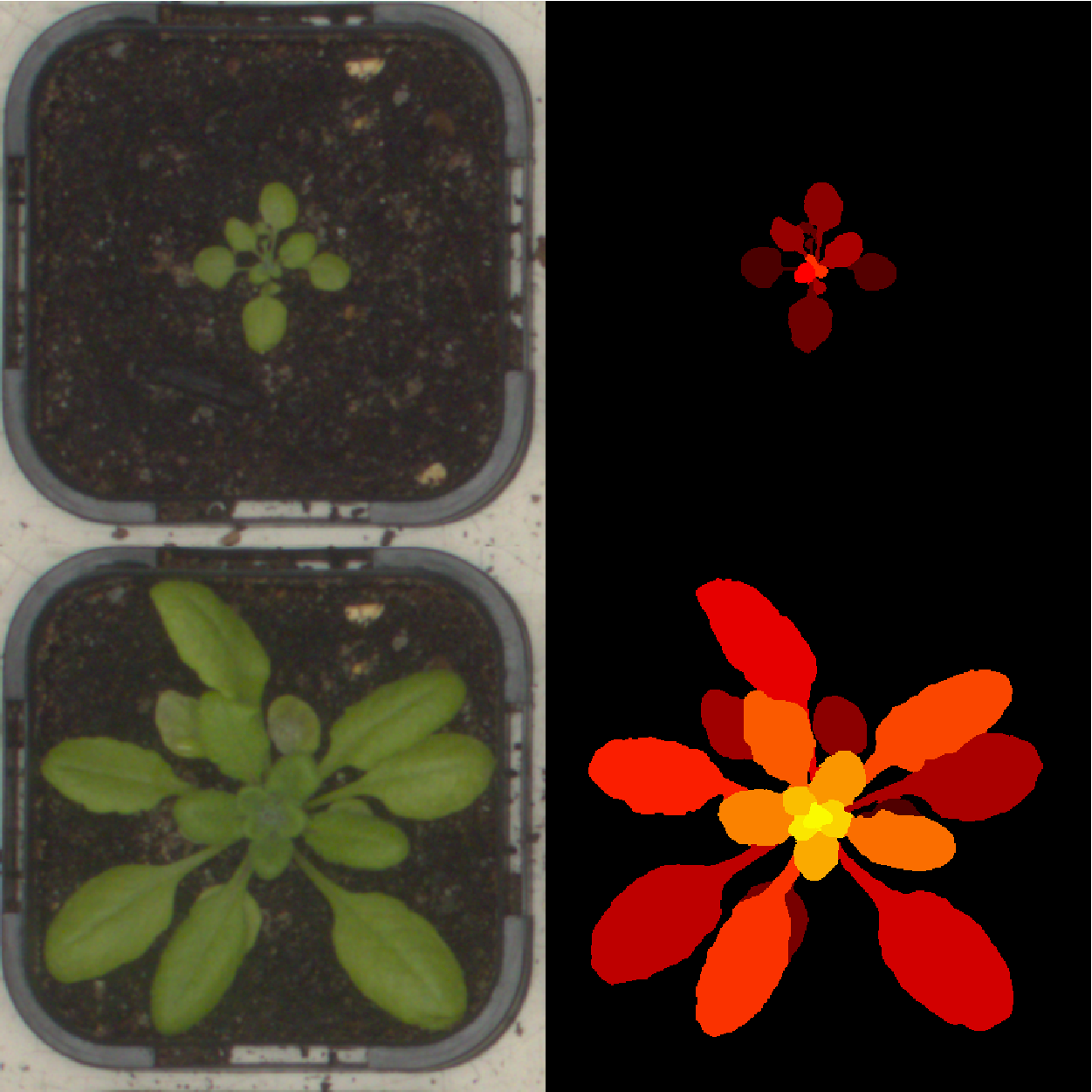
Our dataset has accompanying ground truth annotations of the last image of each day of one tray (number 31), together with the first image taken 21, 28, 35 and 42 days after sowing and the first image taken after 2pm 28, 35, 42 and 49 days after sowing. This amounts to 43 images with between 10 and 20 plants in each image and a total of 706 annotated plant images from tray 031, as shown in the “train” columns of Table 1. The suggestion is that these are used as training data. We also have ground truth annotations of the first image taken of tray 032 and the first image taken after 2pm every third day, starting 22 days after sowing. This adds another 210 plant annotations shown in the “test” columns of Table 1. Ground truth was created through hand annotations of individual leaves, using a drawing package. This annotation was carried out by casually employed postgraduate students.

Table 1: Images in the suggested training and test data sets along with days after sowing information and number of individual plants

Plant count	D.A.S.	Images (train)	Plants (train)	Images (test)	Plants (test)
20	21 22 25 28	12	240	4	80
18	31 34	9	162	2	36
16	37 40	8	120	2	32
14	43 46	7	98	2	28
12	49 52	4	48	2	24
10	55	3	30	1	10
Total		43	706	13	210

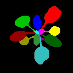
The test set has no plants in common with the training data. The work described here used this test data / training data split. Examples of annotations from early and late in the growth period are shown in Figure 1.

Figure 1: Two views of a plant from our dataset taken 27 and 42 days after sowing together with ground truth annotations.

3.4 Evaluation of segmentation

Alongside the data and annotations we supply software for evaluation of leaf level segmentation that supports the subset-matched Jaccard index and an alternative implementation of symmetrical best Dice, the evaluation measure used in the Leaf Segmentation challenge [10, 23]. There is a fuller description of the subset-matched Jaccard index approach in [24]. In this paper, we use Symmetric Best Dice for quantifying the quality of segmentations for the sake of compatibility with others’ work, such as [12].

4 Method

The starting point for this work was the empirical observation that segmentation techniques based upon objects (for example, leaves) have difficulty distinguishing individual leaves in the presence of heavy occlusion. For example, Yin et al [16, 17] report an impressive technique for leaf segmentation, but acknowledge that it is less reliable in the presence of more than 25% occlusion. With Arabidopsis plants, this level of occlusion will occur long before the plant nears maturity and flowering. For this reason we aim to detect and classify edges in the image, determining whether an edge is an occluding edge or not, and to base our segmentation technique upon edge information rather than upon models of the entire leaf.

There are further advantages to using an edge based approach. It can be expected that an effective edge based approach might outperform an object based approach where there is on overlap leading to considerable occlusion of one leaf as the shape of the overlapping pair of leaves will resemble a single leaf. An example of this appears in Figure 1. An edge based approach should also speed analysis over a sliding-window based technique, as the object based approach will need to classify all pixels in an image while we need only analyse the edge pixels. Finally, when it comes to machine learning methods, large amounts of training data are vital. One plant might provide 12 example leaves for a training algorithm, but hundreds of examples of edge pixels. Thus by concentrating on a smaller part of the plant, we have a richer set of data to work with.

Given detected edges in an image, we also need to distinguish those edges that are internal to the plant from those that are the edges of the plant as a whole and those that occur in the background. So we have a four way classification problem, summarised as follows:-

• Background - any edge wholly outside a plant

• Plant edge - any edge where plant meets background - these delineate the silhouette of the plant.

• Leaf edge - any edge inside a plant that marks where two leaves overlap.

• Internal noise - any edge that is inside a plant and is not an edge separating two overlapping leaves. These might be caused by shadows, specular reflections or venation of a leaf.

We found that conventional machine learning classifiers worked well on distinguishing plant from background but were less successful at distinguishing between leaf edges where one leaf overlaps another and spurious edges found within the area of a plant. While the main interest in this approach to classification is in distinguishing between these last two “inside plant” classes, our approach is very effective at classifying plant edges so is effective for plant from background segmentation.

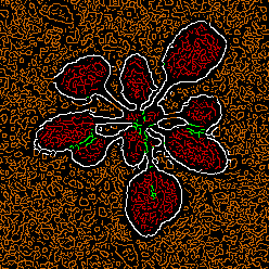
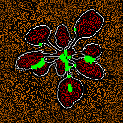
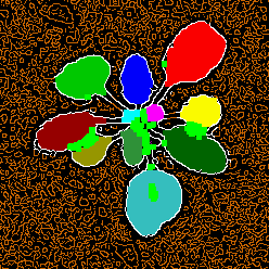
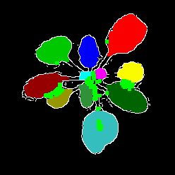
The result of the edge classification process can be visualised as an image rather like a line drawing, as shown in the second element of Figure 3, with each class of edge depicted with a line of different colour. However, for obtaining measurements a region based segmentation with each leaf a different value is preferable, which makes leaf area and leaf count easy to derive. This requirement leads to the main disadvantage of our approach, as we need a second post-classification step to convert our edge classifications to a regional segmentation, complicating the image processing sequence. It is necessary to:-

1. Locate image edges. This is done using the Canny edge detector. The only requirement is that sensitivity is high because as many of the plant and leaf edges should be identified as possible. The classification stage identifies the irrelevant edges, thus overdetection is not important for us.

2. Classify edge pixels into one of the four classes outlined above.

3. Convert the edge based segmentation into a region based one. This can be done using conventional image processing techniques as described in Section 4.2

The effectiveness of our final segmentation and leaf count thus depends not only on the quality of edge classification, but also on how well the edge classifications can be translated to region based classifications.

4.1 Edge classification

Our classification techniques are based upon a convolutional neural network (CNN). Various configurations of this network were tried, and we report performance of the network under some of these configurations in Section 5. The basic configuration is shown in Figure 2.

Figure 2: A simple deep learning network that alternates convolution and pooling layers for four way classification of edge pixels.

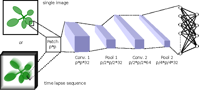
We have experimented with two key variations to the architecture. Firstly, we tried replacing the single four way classification by a tree of binary classifications in which different networks (with identical architectures) are used to first separate the internal edges from the others (i.e. plant edges and background) and then to subdivide each of those sets. Secondly, we investigated “temporal patches”, which build a patch to be classified from a line of pixels normal to the edge, taken from a sequence of time lapse images. The pixels from the same locations in each image are used. This is illustrated in the bottom of Figure 2.

Some further experimental configurations have been tested but did not improve the performance of our classifier, and so are not included in the results section. We mention them here for completeness. These were increasing the final pool output to 64, and doubling the pooling layers (where each convolutional layer is followed by a pair of pooling layers, making the sequence Conv. 1, Pool 1, Pool 2, Conv. 2, Pool 3, Pool 4 before the fully connected classification layer).

4.2 Region based segmentation

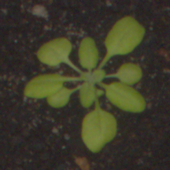
Once we have our edge classifications, this can be treated as an image consisting of lines where each classification of edges is a line of a different colour. In the examples presented here, plant edges are white, leaf edges are green, background edges are orange and internal noise edges are red. However, the required result can be thought of as an image wherein each segmented region (leaf) is an area of a distinct colour, comparable to the ground truth images shown in 1. In both cases, the background is black. We use a sequence of conventional image processing techniques to convert our line image to a region based segmented image from which measurements can be obtained by pixel counting. This is illustrated in Figure 3.

(a) Remove isolated edges

(b) Dilate internal edges

(c) Flood fill

(d) Remove remaining edges

(e) Inflate leaf

(f) Final noise removal

(g) Original Image

(h) Ground Truth

Figure 3: The image processing steps from edge classification to the creation of a leaf-level segmented image. Figures (a) to (f) correspond to steps (a) to (f) in the main text.

The post classification step itself has seven steps, five of which are specific cases of dilation. These steps are:

1. Remove isolated ”spots” of edge pixels classified as either plant edge or leaf edge. Any regions of plant edge or leaf edge pixels that are isolated within a region of 5 by 5 pixels are removed. If any of the pixels around the edge of this region are any colour other than the background colour, the pixels to be replaced are changed to that colour, otherwise they are changed to background colour.

2. Dilate the leaf edges. This reduces discontinuities resulting from the original edge detection step. In essence, the image as treated as binary with leaf edge pixels classed as 1 and all other colours as 0, so any pixel that is within the range of dilation that is not leaf edge coloured is changed to that colour. Again a 5 by 5 region is used.

3. Each distinct internal region (leaf) is coloured using flood fill. Each individual leaf is assigned to its own class (that is, a different colour is used for each leaf). Flood fill is stopped when either leaf edge or plant edge pixels are encountered. A 5 by 5 structuring element is used to find a pixel that triggers the stopping of flood fill, so any remaining holes in edge pixel classifications do not result the flood fill “leaking out”. This also prevents narrow petioles being filled.

4. Background edges are removed, replaced by background colour.

5. The flood filled leaf colours are dilated but only over leaf edge pixels. This continues until all leaf edge coloured pixels are replaced by a leaf colour. Leaf colours are dilated by one, but only over background coloured or plant edge coloured pixels. This would ideally result in the replacement of the plant edges but sometimes isolated pixels remain.

6. Finally, any remaining plant edge coloured pixels are changed to their neighbour’s colour. This will be any leaf colour that two neighbouring pixels share, or background colour if there is no such colour.

This results in a coloured image with a black background and each leaf (as detected by the classification) coloured a different colour, so it can be evaluated against the corresponding ground truth annotation to evaluate the quality of the segmentation. The results are discussed in the next section.

5 Results

Results are presented using the same evaluation measures as in the Leaf segmentation Challenge, [10, 23]. These are Difference in Count (DiC), Absolute Difference in Count ($|$DiC$|$), Foreground/Background Dice (FBD), and Symmetric Best Dice (SBD). With regard to DiC, figures quoted here are mean results from several plants, and so this measure is not very useful as over- and under- segmentation tend to cancel each other out. So the sign of this result here gives an indication of whether the approach tends to over or under segment, but it tells us little else. The standard deviation (quoted in brackets in the tables) is a more useful guide to accuracy in this case. The use of these metrics ensures our results can readily be compared with results in [12].

Results presented here show the effects of varying aspects of our CNN setup relative to a “baseline” configuration. This baseline configuration is as follows:-

• Using a set of three binary classifications rather than one four way classification.

• Using a patch from a single image, not one obtained from normals from a timelapse sequence.

• Using a patch size of 16 pixels square.

• Using the CNN architecture illustrated in Figure 2

Experiments were run using training sets drawn from our dataset, and tested using the test sets as described earlier. Results quoted are the mean of score for plants in one image of our test data set, the image being taken 31 days after sowing; this was chosen as it presents reasonable levels of occlusion and also corresponds closely to the data in the LSC challenge. The results here presented omit those variations in network architecture which made little difference.

Table 2: The effect of CNN parameters quality of leaf counting and segmentation. The asterisked lines represent our baseline configuration, and standard deviations are presented in brackets

Experiment	Variant	DiC	$|$DiC$|$	FBD	SBD
Patch Size	8	5.94 (3.87)	6.06 (3.69)	0.94 (0.01)	0.55 (0.12)
	12	3.94 (3.21)	4.06 (3.06)	0.95 (0.01)	0.63 (0.11)
	16*	1.06 (1.73)	1.39 (1.46)	0.95 (0.01)	0.68 (0.09)
	32	-0.33 (2.30)	1.78 (1.44)	0.95 (0.01)	0.70 (0.08)
Binary vs 4-way	Binary*	1.06 (1.73)	1.39 (1.46)	0.95 (0.01)	0.68 (0.09)
	Four-way	-0.83 (2.31)	2.06 (1.26)	0.94 (0.01)	0.71 (0.07)
Single image vs temporal patch	Single*	1.06 (1.73)	1.39 (1.46)	0.95 (0.01)	0.68 (0.09)
	Temporal	3.78 (4.29)	3.89 (4.19)	0.95 (0.01)	0.61 (0.12)

Increasing the patch size up to 16 improved classification and segmentation. There was little if any further improvement increasing patch size to 32. Increasing the patch size has the drawback that more edge pixels have their associated patches “bleeding off” the edge of the image. In general, better results were obtained from using the binary sequence approach rather than a single four way classification. Finally, the idea of making the patches from a time lapse sequence of images did not reveal any improvement. It also introduces the problem of gaps in the sequence because the use of visible light prevents images being taken at night, leaving 12-hour gaps in the sequence each day.

As Arabidopsis plants grow, the number of leaves increases as does the amount that they overlap so it might be expected that results for leaf counting and measurement will be worse with older plants and Table 3 demonstrates this.

Table 3: The effect of using older plant (37 against 31 days after sowing) on quality of leaf counting and segmentation.

Age of plants	DiC	$|$DiC$|$	FBD	SBD
31 d.a.s.	1.06 (1.73)	1.39 (1.46)	0.95 (0.01)	0.68 (0.09)
37 d.a.s.	-0.94 (6.56)	5.19 (3.90)	0.96 (0.01)	0.58 (0.10)

In addition to the experiments using our own images, some variations were tried with a publicly available subset of the Leaf Segmentation Challenge Dataset, the LSC “A2” dataset, that being the set most similar to ours. The motivation for doing this was to see how dependent our approach is to having training data closely matched to the test data; as there are 31 ground-truthed plants in the LSC A2 dataset there were not enough instances to tailor our model by training our CNN from scratch. Thus our approach, trained on the 706 plants from the ALED dataset, has a similar input to the LSC A2 dataset capture setup but is not a perfect match. We could not try the “temporal patches” variations with this data owing to the lack of time lapse data in the Leaf Segmentation Challenge dataset. In Table 4 we present the baseline variations using our data and the same variations using the LSC data as test date for comparison.

Table 4: Results on the LSC A2 dataset, compared with other techniques as reported in [12], [21] and [20]. Asterisked results are aggregated over all LSC datasets, rather than just L2.

Method	DiC	$|$DiC$|$	FBD	SBD
Our method	-0.3 (2.3)	1.8 (1.4)	0.95 (0.01)	0.70 (0.08)
ITK	-1.0 (1.5)	1.2 (1.3)	0.96 (0.01)	0.77 (0.08)
Nottingham	-1.9 (1.7)	1.9 (1.7)	0.93 (0.04)	0.71 (0.1)
MSU	-2.0 (1.5)	2.0 (1.5)	0.88 (0.36)	0.66 (0.08)
Wageningen	-0.2 (0.7)	0.4 (0.5)	0.95 (0.2)	0.76 (0.08)
Romera-Paredes*	0.2 (1.4)	1.1 (0.9)	N/A	0.57 (0.8)
Romera-Paredes+CRF*	0.2 (1.4)	1.1 (0.9)	N/A	0.67 (0.9)
Ren*	N/A	0.8 (1.0)	N/A	0.85 (0.5)

6 Discussion

Our results are not dissimilar from those achieved by the approaches covered in [12], and also those achieved by [20] although a direct comparison is impossible due to differences in datasets. With the exception of [20] all methods were trained on the LSC data, and ours was not. Ren and Zemel, in [21], present considerably better results exceeding the current state-of-the-art on counting and symmetric best dice using a general purpose object counting network (RNN); parts of this system are pre-trained and this approach to learning shows a lot of promise.

While our approach does well at plant from background segmentation, there is still room for improvement in the leaf level results.

In the hope of establishing to what extent our results are attributable to the use of CNNs, we tried a Random Forest classifier (as implemented in Weka) to classify edges using patches. Table 5 shows these results, and it is clear that using a CNN gave a noticeable improvement in leaf count and symmetric best dice. These results do raise the possibility of using a simpler classifier for plant from background segmentation with a single CNN for classifying the two groups of edges found within the plant - overlapping leaf edges and others.

Table 5: Comparison of results using the CNN and Random Forest on the same image with the same patch size (12).

Classifier	DiC	$|$DiC$|$	FBD	SBD
CNN	1.4 (2.51)	1.8 (2.17)	0.95 (0.01)	0.70 (0.13)
Random Forest	-2.4 (4.16)	3.6 (2.88)	0.95 (0.01)	0.53 (0.13)

Most approaches using deep learning use objects rather than edges as the feature to be classified. There seem to us to be advantages in using edges, at least for the problem we set out to solve. If the leaf is taken as the object to be classified, this is of variable shape and size, quite apart from the problem of occlusion as the plant grows more leaves. Many object based approaches appear to struggle once one of a pair of leaves is largely hidden. As the percentage of overlap increases, the overall shape of a pair of leaves more closely resembles a possible single leaf shape, so an object based system might not detect the existence of a second leaf, while the approach described here should.

When developing useful plant phenotyping systems, there are many considerations besides the range and accuracy of measurements obtainable from a system. We consider the criteria listed in [23] an excellent set of characteristics for working in an interdisciplinary setting; in particular their emphasis on robustness and automation are key for high throughput work. The approach described herein goes some way to meeting many these:

1. Accommodate most laboratory settings. We were able to obtain results on the LSC A2 dataset (which we had not trained the CNNs on) that approach the results we obtained on our own dataset. This shows the approach is reasonably flexible with respect to differences in set-up out of the box.

2. Not rely on an explicit scene arrangement. The method we have developed is tailored to top-down views of rosette plants in trays, and we do not expect it to work that well on other species or camera configurations. However top-down imaging such as we analyse here is a very common setup for rosette plants.

3. Handle multiple plants in an image. It does this, using high throughput phenotyping images with up 20 plants in an image.

4. Tolerate low resolution and out of focus discrepancies. The camera used was 5 Megapixels, by no means high by modern standards, and this resolution was shared by up 20 plants. The camera was used as is, with slight focus discrepancies and barrel distortion.

5. Be robust to changes in the scene. This is not something we have tested, given our robotic capture setup.

6. Require minimal user interaction, in both setting up and training. This is not clear at present. It depends on whether the CNNs could be trained on images from several sources and give good performance on each source, which remains a direction for future work.

7. Be scalable to large populations or high sampling rates. It is likely that this would depend on the computing power available, but as the technique is non-interactive, computer resource is the bottleneck (there is no human in the loop).

8. Offer high accuracy and consistent performance. This is good for plant from background segmentation but there is room for improvement at the leaf level, as discussed earlier.

9. Be automated with high throughput. Once trained the approach is entirely automated.

6.1 Future work

One limitation of the work imposed by the nature of the available data is that the CNNs were trained on data from the same capture setup as the test data. This obvious issue is driven by the need to train the CNNs on a large, labelled dataset. The broader utility of the system would depend on how well a CNN trained on images from multiple sources would work. We show some positive results in the direction of cross-dataset transferability (networks trained upon the ALED dataset performing well on the LSC), but we acknowledge that this is an area for future development.

We have made the datasets we used for this work publicly available and encourage other researchers in the field to do the same, as sufficient publicly available datasets will be invaluable in advancing the state of the art. Given the dominance of CNN-based imaging techniques in computer vision, and the reliance of such techniques on large quantities of training data, the dataset question is a becoming major one. The presence of more, larger datasets such as ALED can only help here.

With regard to deployment, it would be possible to train the network as it stands as part of the installation process for a phenotyping system. In this case, the installed system could in a sense be tuned to images from a particular capture setup. This is clearly not ideal, especially as a large set of ground truth data would be needed, but might be a good solution for larger phenotyping installations.

As we are not reliant on models of leaf shape, it seems reasonable to expect that the approach might be readily usable with other rosette plants beside Arabidopsis. It would be interesting to test the approach against datasets of other plants and especially against data sets of multiple plant species for both training and test data. Again, lack of available data has prevented this at the current time, although this is certainly the direction of our future work plans.

7 Conclusion

The method of image analysis presented here appears to offer performance comparable to the current state of the art. Results for plant from background segmentation are encouraging and our leaf counting results seem to offer an improvement over many of those in [12].

While there remains scope for improvement in both leaf counting and leaf segmentation performance we suggest that the approach offers a route towards further developments and that such developments will be both encouraged and enabled by the release of our data set and accompanying annotations to the wider community. We hope other researchers will do the same. The potential benefits of automated image analysis for phenotyping amply justify the continued development of work such as that presented here.

Availability of data and material

The dataset is hosted at https://zenodo.org and it can be found from https://doi.org/10.5281/zenodo.168158.

References

- [1] J. De Vylder, D. Ochoa, W. Philips, L. Chaerle, and D. Van Der Straeten, “Leaf segmentation and tracking using probabilistic parametric active contours,” in Computer Vision/Computer Graphics Collaboration Techniques, ser. Lecture Notes in Computer Science, A. Gagalowicz and W. Philips, Eds. Springer Berlin Heidelberg, 2011, vol. 6930, pp. 75–85.
- [2] R. T. Furbank and M. Tester, “Phenomics – technologies to relieve the phenotyping bottleneck,” Trends in Plant Science, vol. 16, no. 12, pp. 635–644, Dec. 2011.
- [3] S. Dhondt, N. Gonzalez, J. Blomme, L. De Milde, T. Van Daele, D. Van Akoleyen, V. Storme, F. Coppens, Beemster, and D. Inzé, “High-resolution time-resolved imaging of in vitro Arabidopsis rosette growth,” The Plant Journal, vol. 80, no. 1, pp. 172–184, Oct. 2014.
- [4] W. Engelmann, K. Simon, and C. J. Phen, “Leaf movement rhythm in Arabidopsis thaliana,” Zeitschrift für naturforchung C, vol. 47, no. 11–12, pp. 925–928, 1992.
- [5] J. Bell and H. Dee, “Watching plants grow - a position paper on computer vision and Arabidopsis thaliana,” IET Computer Vision, 2016, doi:10.1049/iet-cvi.2016.0127.
- [6] D. Leister, C. Varotto, P. Pesaresi, A. Niwergall, and F. Salamini, “Large-scale evaluation of plant growth in Arabidopsis thaliana by non-invasive image analysis,” Plant Physiology and Biochemistry, vol. 37, no. 9, pp. 671–678, Sep. 1999.
- [7] D. C. Boyes, A. M. Zayed, R. Ascenzi, A. J. McCaskill, N. E. Hoffman, K. R. Davis, and J. Görlach, “Growth stage-based phenotypic analysis of Arabidopsis: a model for high throughput functional genomics in plants.” The Plant Cell, vol. 13, no. 7, pp. 1499–1510, Jul. 2001.
- [8] M. Minervini, M. V. Giuffrida, and S. Tsaftaris, “An interactive tool for semi-automated leaf annotation,” in Proceedings of the Computer Vision Problems in Plant Phenotyping (CVPPP), S. A. Tsaftaris, H. Scharr, and T. Pridmore, Eds. BMVA Press, Sep. 2015, pp. 6.1–6.13. [Online]. Available: https://dx.doi.org/10.5244/C.29.CVPPP.6
- [9] M. Minervini, A. Fischbach, H. Scharr, and S. A. Tsaftaris, “Finely-grained annotated datasets for image-based plant phenotyping,” Pattern Recognition Letters, vol. 81, pp. 80–89, 2016, doi: 10.1016/j.patrec.2015.10.013.
- [10] H. Scharr, M. Minervini, A. Fischbach, and S. A. Tsaftaris, “Annotated Image Datasets of Rosette Plants,” Institute of Bio- and Geosciences: Plant Sciences (IBG-2), Forschungszentrum Jülich GmbH, Jülich, Germany, Tech. Rep. -, 2014. [Online]. Available: http://juser.fz-juelich.de/record/154525
- [11] J. A. Cruz, X. Yin, X. Liu, S. M. Imran, D. D. Morris, D. M. Kramer, and J. Chen, “Multi-modality imagery database for plant phenotyping,” Machine Vision and Applications, vol. 27, no. 5, pp. 735–749, 2016. [Online]. Available: http://dx.doi.org/10.1007/s00138-015-0734-6
- [12] H. Scharr, M. Minervini, A. P. French, C. Klukas, D. M. Kramer, X. Liu, I. Luengo, J.-M. Pape, G. Polder, D. Vukadinovic, X. Yin, and S. A. Tsaftaris, “Leaf segmentation in plant phenotyping: a collation study,” Machine Vision and Applications, vol. 27, no. 4, pp. 585–606, May 2016.
- [13] J.-M. Pape and C. Klukas, “3-D histogram-based segmentation and leaf detection for rosette plants,” in Computer Vision - ECCV 2014 Workshops, ser. Lecture Notes in Computer Science, L. Agapito, M. M. Bronstein, and C. Rother, Eds. Springer International Publishing, 2015, vol. 8928, pp. 61–74.
- [14] ——, “Utilizing machine learning approaches to improve the prediction of leaf counts and individual leaf segmentation of rosette plant images,” in Proceedings of the Computer Vision Problems in Plant Phenotyping (CVPPP), S. A. Tsaftaris, H. Scharr, and T. Pridmore, Eds. BMVA Press, September 2015, pp. 3.1–3.12. [Online]. Available: https://dx.doi.org/10.5244/C.29.CVPPP.3
- [15] D. Vukadinovic and G. Polder, “Watershed and supervised classification based fully automated method for separate leaf segmentation,” in The Netherlands Conference on Computer Vision, 2015.
- [16] X. Yin, X. Liu, J. Chen, and D. M. Kramer, “Multi-leaf tracking from fluorescence plant videos,” in 2014 IEEE International Conference on Image Processing (ICIP). IEEE, Oct. 2014, pp. 408–412.
- [17] ——, “Multi-leaf alignment from fluorescence plant images,” in 2014 IEEE Winter Conference on Applications of Computer Vision (WACV). IEEE, Mar. 2014, pp. 437–444.
- [18] Y. LeCun, Y. Bengio, and G. Hinton, “Deep learning,” Nature, vol. 521, pp. 436–444, May 2015.
- [19] M. P. Pound, A. J. Burgess, M. H. Wilson, J. A. Atkinson, M. Griffiths, A. S. Jackson, A. Bulat, G. Tzimiropoulos, D. M. Wells, E. H. Murchie, T. P. Pridmore, and A. P. French, “Deep machine learning provides state-of-the-art performance in image-based plant phenotyping,” bioRxiv, 2016. [Online]. Available: http://biorxiv.org/content/early/2016/05/12/053033
- [20] B. Romera-Paredes and P. H. Torr, “Recurrent instance segmentation,” in European Conference on Computer Vision (ECCV) 2016, 2016, ArXiv preprint ArXiv:1511.08250v2.
- [21] M. Ren and R. S. Zemel, “End-to-end instance segmentation and counting with recurrent attention,” in Computer Vision and Pattern Recognition, July 2017, pp. 6656–6664.
- [22] “Photon Systems Instruments PlantScreen Phenotyping,” http://psi.cz/products/plantscreen-phenotyping/ (accessed 13/4/2016).
- [23] M. Minervini, M. M. Abdelsamea, and S. A. Tsaftaris, “Image-based plant phenotyping with incremental learning and active contours,” Ecological Informatics, vol. 23, pp. 35–48, Sep. 2014.
- [24] J. Bell and H. M. Dee, “The subset-matched Jaccard index for evaluation of segmentation for plant images,” Department of Computer Science, Aberystwyth University, Tech. Rep., 2016, available at: https://arxiv.org/abs/1611.06880. [Online]. Available: https://arxiv.org/abs/1611.06880