Reliable estimation of the radius of convergence in finite density QCD

Abstract

We study different estimators of the radius of convergence of the Taylor series of the pressure in finite density QCD. We adopt the approach in which the radius of convergence is estimated first in a finite volume, and the infinite-volume limit is taken later. This requires an estimator for the radius of convergence that is reliable in a finite volume. Based on general arguments about the analytic structure of the partition function in a finite volume, we demonstrate that the ratio estimator cannot work in this approach, and propose three new estimators, capable of extracting reliably the radius of convergence, which coincides with the distance from the origin of the closest Lee-Yang zero. We also provide an estimator for the phase of the closest Lee-Yang zero, necessary to assess whether the leading singularity is a true critical point. We demonstrate the usage of these estimators on a toy model, namely 4 flavors of unimproved staggered fermions on a small $6^{3}\times 4$ lattice, where both the radius of convergence and the Taylor coefficients to any order can be obtained by a direct determination of the Lee-Yang zeros. Interestingly, while the relative statistical error of the Taylor expansion coefficients steadily grows with order, that of our estimators stabilizes, allowing for an accurate estimate of the radius of convergence. In particular, we show that despite the more than 100% error bars on high-order Taylor coefficients, the given ensemble contains enough information about the radius of convergence.

I Introduction

One of the most important unsolved problems in QCD is the determination of its phase diagram at finite baryonic density. In particular, an open question is whether the analytic crossover of the chiral transition at zero chemical potential turns into a genuine phase transition sufficiently deep in the $\mu-T$ (chemical potential-temperature) plane, and, if so, where the critical endpoint lies. Nonperturbative studies of these questions on the lattice are notoriously hampered by the sign problem, which prevents the use of standard Monte Carlo techniques to probe QCD directly at finite density. Reweighting techniques Hasenfratz and Toussaint (1992); Barbour et al. (1998); Fodor and Katz (2002a, b, 2004); Csikor et al. (2004) shift this problem from the integration measure to the observable, allowing the use of standard Monte Carlo techniques, but they are still limited in scope by the sign and overlap problems, both of which are exponentially hard in the lattice volume. At the moment, the state of the art for lattices close to the continuum limit is to calculate Taylor coefficients of the pressure, either by direct calculations at $\mu=0$  Allton et al. (2002, 2005); Gavai and Gupta (2008); Basak et al. (2008); Borsányi et al. (2012a, b); Bellwied et al. (2015); Ding et al. (2015); Bazavov et al. (2017) or via fitting a polynomial ansatz to results obtained with simulations at zero and imaginary chemical potentials de Forcrand and Philipsen (2002); D’Elia and Lombardo (2003); D’Elia and Sanfilippo (2009); Bonati et al. (2014, 2015); D’Elia et al. (2017); Günther et al. (2017); Vovchenko et al. (2017); Bonati et al. (2018); Borsányi et al. (2018). When trying to infer if the calculated Taylor coefficients show any sign of criticality, a common choice is to use simple estimators of the radius of convergence, like the ratio estimator D’Elia et al. (2017); Bazavov et al. (2017); Fodor et al. (2018). The purpose of this paper is to obtain some insight on the usefulness of such estimators, using both analytical and numerical methods.

The study of the radius of convergence $r$ from the Taylor coefficients can be carried out in two different ways. One is to perform first the infinite volume extrapolation of every coefficient, and in the next step estimate the radius of convergence from the large-order limit of an appropriate estimator. In other words, given an estimator $R_{n}(V)$ of $r$, where $V$ is the volume of the system and $n$ is the order of the Taylor expansion, one determines $r$ by taking limits in the order $r=\lim_{n\to\infty}\lim_{V\to\infty}R_{n}(V)$. The other procedure is to estimate the radius of convergence in a finite volume first, and in the next step do the infinite volume extrapolation, i.e., taking limits in the order $r=\lim_{V\to\infty}\lim_{n\to\infty}R_{n}(V)$. While both approaches are valid and worth being investigated, in this paper we will focus on the latter, mainly for the following reasons.

First, in a finite volume, the analytic form of the large-order behavior of the Taylor expansion of the pressure is particularly simple, allowing us to produce analytical arguments about the accuracy and reliability of different convergence radius estimators, which we will proceed to do in this paper.

Second, the infinite-volume extrapolation in finite density QCD is very hard, mainly because the sign problem is exponentially hard in the volume. Any fixed-order calculation of the Taylor coefficients has only polynomial complexity in the volume, but the order of the polynomial increases with the order of the coefficient, eventually recovering the full exponential complexity in the infinite-order limit. This makes it useful to study methods that can give well defined results already in a finite volume.

In a finite volume, the radius of convergence coincides with the distance from the origin of the closest Lee-Yang zero Lee and Yang (1952), i.e., the zero of the partition function closest to the origin in the complex $\mu$ plane. The behavior of Lee-Yang zeros in the thermodynamic limit provides very useful information about the phase diagram of the theory. In fact, the presence of a critical point is signaled by Lee-Yang zeros reaching somewhere the real $\mu$ axis in the infinite-volume limit. The rate at which the real axis is approached tells us about the nature and the strength of the transition: in particular, a first order phase transition is signaled by the imaginary part of the nearby Lee-Yang zeros vanishing like $1/V$. The large-volume limit of the real part of such zeros determines of course the location of the critical point. Zeros that even in the thermodynamic limit remain a finite but small distance away from the real axis are expected to correspond to an analytic crossover. It is clear that while the Lee-Yang zeros determine both the critical points (if any) of the theory and the radius of convergence of the Taylor series of the pressure, nothing guarantees that the same zeros are involved in the two cases. Nonetheless, this is entirely possible, and in the worst case the radius of convergence provides a lower bound on the critical endpoint.

In this paper we study whether one can accurately infer the position of the leading Lee-Yang zero from the Taylor coefficients of the pressure, assessing the reliability of the various radius estimators and their computational cost. In Section II we discuss Lee-Yang zeros in QCD in some detail, relate them to the Taylor coefficients of the pressure, and exploit their symmetries to assess the viability of the ratio estimator, and of three new proposals to estimate the radius of convergence. We also discuss Fisher zeros, i.e., zeros of the partition function in the complex gauge coupling plane, and show how they relate to the cumulants of the gauge action. In Section III we test our arguments by computing all the Lee-Yang zeros in a toy model for lattice QCD, namely $N_{f}=4$ unimproved unrooted staggered fermions on a small, $6^{3}\times 4$ lattice, and comparing the radius of convergence extracted from the Taylor coefficients to the known position of the closest Lee-Yang zero. To further test our methods, we apply our convergence radius estimators to find the Fisher zero closest to the real axis, and compare it with a direct determination using reweighting. Our conclusions are presented in Section IV.

II Lee-Yang zeros, Taylor series in a finite volume, and convergence radius estimators

We will study the convergence of several different Taylor series expansions of the pressure $p=\frac{T}{V}\log Z$, where $Z$ is the grand canonical partition function. For a relativistic theory on the lattice in a finite volume, $Z$ reads:

$$Z(\hat{\mu})={\sum}_{n=-kV}^{+kV}Z_{n}e^{n\hat{\mu}}\,.$$ (1)

Here $\hat{\mu}=\mu/T$, $V=N_{s}^{3}$ is the lattice volume, $Z_{n}$ are temperature-dependent real positive coefficients, and $k$ is a constant depending on the particular model. The coefficients $Z_{n}$ are the canonical partition functions, corresponding to the sector of Hilbert space where the conserved charge conjugated to $\mu$ equals $n$. In the case of the model to be discussed below in Section III, i.e., $N_{f}=4$ lattice QCD with unrooted staggered fermions, we have $k=3$.

The partition function is a non-vanishing analytic function of $\hat{\mu}$ (i.e., $e^{-kV\hat{\mu}}$) times a polynomial of order $2kV$ in the fugacity $e^{\hat{\mu}}$, and by the fundamental theorem of algebra it has $2kV$ roots in the complex fugacity plane, called Lee-Yang zeros Lee and Yang (1952). In terms of the Lee-Yang zeros the partition function can be written as follows,

$$Z(\hat{\mu})=\text{non-vanishing\ }\cdot\prod_{m=1}^{2kV}(\Lambda_{m}-e^{\hat{\mu}})\,.$$ (2)

The logarithm of the partition function therefore has the form:

$$\frac{pV}{T}=\log Z(\hat{\mu})=\text{analytic\ }+\sum_{m=1}^{2kV}\log(\Lambda_{m}-e^{\hat{\mu}})\,.$$ (3)

Since the finite-volume partition function as a function of $\hat{\mu}$ is a finite sum of exponentials, and so an entire function, the Weierstrass factorization theorem (see, e.g., Ref. Rudin (1997)) states that a similar factorization also exists in terms of $\hat{\mu}$, except that now one has an infinite product. As a function of $\hat{\mu}$, $\log Z$ has therefore the same form as Eq. (3), with the finite sum replaced by an infinite one:

$$\log Z(\hat{\mu})=\text{analytic\ }+\sum_{m=1}^{\infty}\log(\lambda_{m}-\hat{\mu})\,.$$ (4)

This can be easily understood by noticing that to each $\Lambda_{m}$ corresponds an infinite tower of Lee-Yang zeros $\lambda_{m,n}={\rm Log}\,\Lambda_{m}+2\pi ni$, where ${\rm Log}$ is the principal branch of the complex logarithm. Explicitly, to each term in the expansion in fugacity correspond the following terms in the expansion in $\hat{\mu}$:

$$\log\left(e^{\hat{\mu}}-\Lambda\right) =\frac{\hat{\mu}}{2}+\frac{1}{2}{\rm Log}\Lambda+{\rm Log}\left(\hat{\mu}-\rm{Log}\Lambda\right)+$$ (5)

$$+\sum_{k=1}^{\infty}\left[\log(\hat{\mu}-\rm{Log}\Lambda+i2\pi k)-\log(2\pi k)\right]$$

$$+\sum_{k=1}^{\infty}\left[\log(\hat{\mu}-\rm{Log}\Lambda-i2\pi k)-\log(2\pi k)\right]\,,$$

as can be easily worked out by noticing that $e^{\hat{\mu}}-\Lambda=2e^{\hat{\mu}/2}\sqrt{\Lambda}\sinh(\frac{\hat{\mu}}{2}-\frac{1}{2}\rm{Log}\Lambda)$ and utilizing $\sinh(x)=x\prod_{k=1}^{\infty}\left(1+\frac{x^{2}}{\pi^{2}k^{2}}\right)$.

The large-order behavior of the Taylor series of $\log Z$ will be determined by the location of the logarithmic singularity closest to the expansion point in Eqs. (3) or (4). The relevant choices are here $e^{\hat{\mu}}=1$ or $\hat{\mu}=0$, respectively. The two types of expansion can be treated similarly. In both cases the relevant contributions to the partition function have the Taylor series

$$\log(A-x)=\log A+\sum_{k=1}^{\infty}\frac{-1}{k}\frac{1}{A^{k}}x^{k}=b_{0}+\sum_{k=1}^{\infty}b_{k}x^{k}\,,$$ (6)

where the expansion parameter $x$ is either the “fugacity parameter” $\zeta\equiv e^{\hat{\mu}}-1$ or the chemical potential over temperature $\hat{\mu}$, and the relevant Lee-Yang zero $A$ is correspondingly $\Lambda_{1}-1$ or $\lambda_{1}$, having assigned the index $m=1$ to the leading singularity.

The discussion above is rather general. In the specific case of QCD, on which we will be focussing our attention from now on, the symmetries of the theory imply useful relations for the grand canonical partition function $Z(\hat{\mu})$ and for the canonical partition functions $Z_{n}$. Due to CP symmetry (at zero $\theta$-angle), one finds $Z(-\hat{\mu})=Z(\hat{\mu})$ (for complex $\hat{\mu}$), and $Z_{-n}=Z_{n}$. As we have already mentioned above, the $Z_{n}$ are real, which implies that $Z$ is a real analytic function, $Z(\hat{\mu}^{*})=Z(\hat{\mu})^{*}$. It is easy to see that $Z$ is $2\pi$-periodic in the imaginary direction, $Z(\hat{\mu}+i2\pi)=Z(\hat{\mu})$, and furthermore, thanks to the Roberge-Weiss symmetry Roberge and Weiss (1986), one finds $Z(\hat{\mu}+i2\pi/3)=Z(\hat{\mu})$. This implies that the $Z_{n}$ vanish if $n$ is not a multiple of 3. Combining this with the $\hat{\mu}\to-\hat{\mu}$ symmetry, one also concludes that $Z(\hat{\mu}+i\pi/3)=Z(-\hat{\mu}+i\pi/3)$. These properties imply useful symmetries for the distribution of Lee-Yang zeros in the complex plane. In the complex fugacity plane, such a distribution is invariant under reflection through the real axis ($\Lambda\to\Lambda^{*}$), inversion with respect to the unit circle ($\Lambda\to 1/\Lambda$), and rotations of multiples of $\frac{2\pi}{3}$ ($\Lambda\to e^{i\frac{2\pi}{3}}\Lambda$). It is thus sufficient to focus on the region $\{z=re^{i\theta}|~{}r\leq 1\,,~{}~{}0\leq\theta\leq\pi/3\}$ in the complex fugacity plane to determine completely the Lee-Yang zeros of the partition function. In general, due to the positivity of the canonical partition functions $Z_{n}$, no zeros will be found on the real $\hat{\mu}$ axis, and so on the real positive fugacity axis. In the case of QCD with staggered fermions, the fermionic determinant appearing in the functional-integral representation of the partition function is positive definite for purely imaginary $\hat{\mu}$, and so no zeros will appear on the imaginary $\hat{\mu}$ axis, or equivalently on the unit circle in the complex fugacity plane.

II.1 The failure of the ratio estimator

A common estimator for the radius of convergence $r$ of a power series $f(x)=\sum_{k}B_{k}x^{k}$ is the ratio estimator $R_{k}\equiv|B_{k}/B_{k+1}|$, from which one obtains $r$ as $r=\lim_{k\to\infty}R_{k}$ when this limit exists. In the case of the QCD partition function, one naively expects that in the limit of large order $R_{k}$ will be dominated by a single term like that in Eq. (6), thus converging to

$$R_{k}\to\left|\frac{b_{k}}{b_{k+1}}\right|=\left|\frac{(k+1)A^{k+1}}{kA^{k}}\right|\mathop{\to}_{k\to\infty}|A|\,,$$ (7)

as $k\to\infty$. However, a more careful analysis of the analytic structure of the partition function shows that this is not the case. Let us look first at the case of the expansion in the fugacity parameter $\zeta=e^{\hat{\mu}}-1$. Since $Z(\hat{\mu}^{*})=Z(\hat{\mu})^{*}$ and $\zeta(\hat{\mu}^{*})=\zeta(\hat{\mu})^{*}$, the Lee-Yang zeros come in complex-conjugate pairs. There are then two leading singularities, giving the following contributions to the partition function,

$$\log(A-\zeta)+\log(A^{*}-\zeta)$$ (8)

$$=\log A+\log A^{*}+\sum_{k=1}^{\infty}\frac{-2}{k}\frac{\cos(k\theta)}{r^{k}}\zeta^{k}$$

$$=c^{(\zeta)}_{0}+\sum_{k=1}^{\infty}c^{(\zeta)}_{k}\zeta^{k}\,,$$

where $r$ and $\theta$ are the polar coordinates of $A=\Lambda_{1}-1=re^{i\theta}$ in the complex plane. Here it is understood that $|\Lambda_{1}|<1$. The ratio estimators are then:

$$R_{k}^{(\zeta)}=\left|\frac{c^{(\zeta)}_{k}}{c^{(\zeta)}_{k+1}}\right|=r\,\frac{k+1}{k}\left|\frac{\cos(k\theta)}{\cos((k+1)\theta)}\right|\,.$$ (9)

Due to the last factor in this expression, the ratio estimators will never converge in a finite volume for $\theta\neq 0,\pm\pi/2,\pi$. Of course, in a finite volume we never have $\theta=0$ or $\pi$, due to the strict positivity of the partition function. Even in an infinite volume the ratio estimators will not converge, unless $\theta$ converges to one of the values $0,\pm\pi/2,\pi$. Luckily enough, these include the physically interesting case of a genuine phase transition (in this case corresponding to $\theta=\pi$ and $r<1$). On the other hand, the ratio estimator will not work for a general crossover transition corresponding to a complex singularity even in the thermodynamic limit (except for the very special case $\theta=\pm\pi/2$). In this case, even if a genuine phase transition at real $\mu$ exists, but is not the closest singularity to $\zeta=0$, the ratio estimators will not converge, and so will not even give a lower limit on the location of the critical point.

The situation is very similar when expanding in $\hat{\mu}$, except that, since $Z(\hat{\mu})=Z(-\hat{\mu})$, we now have to take into account four Lee-Yang zeros at the same distance from the expansion point, so that the Taylor expansion reads

$$\log(A-\hat{\mu})+\log(A^{*}-\hat{\mu})+\log(-A-\hat{\mu})+\log(-A^{*}-\hat{\mu})$$ (10)

$$=\log A+\log A^{*}+\log(-A)+\log(-A^{*})+$$

$$+\sum_{k=1}^{\infty}\frac{-2}{k}\frac{\cos(k\theta)+\cos(k(\pi-\theta))}{r^{k}}\hat{\mu}^{k}$$

$$=c^{(\hat{\mu})}_{0}+\sum_{k=1}^{\infty}c^{(\hat{\mu})}_{k}\hat{\mu}^{2k}\,.$$

Here $A=\lambda_{1}=re^{i\theta}$, and it is understood that $0\leq\theta\leq\frac{\pi}{2}$. The expansion coefficients of course vanish for odd order, corresponding to the fact that the pressure is an even function of the chemical potential. The ratio estimators read in this case

$$\left(R_{k}^{(\hat{\mu})}\right)^{2}=\left|\frac{c^{(\hat{\mu})}_{k}}{c^{(\hat{\mu})}_{k+1}}\right|=r^{2}\,\frac{k+1}{k}\left|\frac{\cos(2k\theta)}{\cos(2(k+1)\theta)}\right|\,.$$ (11)

This is essentially the same formula as for the fugacity parameter, up to the substitutions $r\to r^{2}$ and $\theta\to 2\theta$, and therefore exactly the same comments apply. In particular, the ratio estimator will work only if $\theta=0,\frac{\pi}{4},\frac{\pi}{2}$, which include (in the thermodynamic limit) genuine phase transitions at real or purely imaginary $\mu$, of course in case that they correspond to the closest singularity.

The similarity between the two cases is made even clearer if one realizes that $Z(\hat{\mu})$ is, in fact, an entire function of $\hat{\mu}^{2}$, as a consequence of the symmetry $Z_{n}=Z_{-n}$ of the QCD canonical partition functions. One can then repeat the discussion in terms of $\hat{\mu}^{2}$, starting from Weierstrass factorization and noticing that the roots are now nothing but $\lambda_{m}^{2}$, and come in complex conjugate pairs. This leads directly to Eq. (LABEL:eq:taylor_1ly_mu) for the contribution of the leading pair of singularities, which is manifestly an expansion in $\hat{\mu}^{2}$. It is evident that the Taylor coefficients $c_{k}^{(\zeta)}$ and $c_{k}^{(\hat{\mu})}$ have the same form when the latter are expressed in terms of the polar coordinates of the leading zero in $\hat{\mu}^{2}$, i.e., $\lambda_{1}^{2}$, which is understood to lie in the upper half of the complex $\hat{\mu}^{2}$-plane.

One final comment: the leading Lee-Yang zero for the two expansions need not be the same, i.e., in general $e^{\lambda_{1}}\neq\Lambda_{1}$, since changing the expansion parameter corresponds to a conformal map on the complex chemical potential plane, that can change the ordering of the distances of the singularities from the origin. Such a situation of changing the ordering of the singularities was pointed out for the example of a chiral effective model in Ref. Skokov et al. (2011).

II.2 Fisher zeros and cumulants of the gauge action

A rather similar argument applies if, instead of the chemical potential $\hat{\mu}$, one considers the gauge coupling $\beta$ as a complex variable. One starts by writing the lattice partition function in its path-integral representation,

$$Z(\beta)=\int\mathcal{D}Ue^{-\beta G}\det M\,,$$ (12)

where $\mathcal{D}U$ denotes invariant group integration of the gauge links, $G$ is the $\beta$-independent gauge action, and $M$ is the fermion matrix. For a finite number of SU(3) integrals $Z$ is an entire function of the gauge coupling $\beta$. Complexifying the coupling as $\beta\to\beta_{C}=\beta+w$ with $\beta$ kept real, having in mind to perform simulations at $\beta$, one can exploit Weierstrass factorization to write

$$Z(\beta+w)\equiv f(w)=f(0)e^{w\frac{f^{\prime}(0)}{f(0)}}\prod_{k}\left[\left(1-\frac{w}{w_{k}}\right)e^{w/w_{k}}\right]\,,$$ (13)

where the product runs over all roots $w_{k}$ of the entire function $f$. The Fisher zeros, i.e., the zeros of $Z$, are easily identified as $\beta_{k}=\beta+w_{k}$. The Taylor coefficients $c_{n}^{(\beta)}$ of the expansion of $f(w)$ in $w$, or equivalently the Taylor coefficients of $\log Z$ in the gauge coupling variable around the simulation point $\beta$, are nothing but the cumulants of the gauge action up to numerical factors,

$$c^{(\beta)}_{n} =\frac{(-1)^{n}}{n!}\llangle G^{n}\rrangle\,,$$ (14)

$$\llangle G^{n}\rrangle \equiv(-\partial_{\beta})^{n}\log Z(\beta)\,.$$

Using Eq. (13) we can then relate cumulants and Fisher zeros as follows,

$$\llangle G^{n}\rrangle=-(n-1)!\sum_{k}\frac{1}{(\beta_{k}-\beta)^{n}}\quad\quad(n\geq 2)\,.$$ (15)

If the quark determinant is real, in particular for $\mu=0$, we have the same symmetry we had with $\zeta$ and $\hat{\mu}^{2}$, i.e., Fisher zeros also come in complex conjugate pairs, and at high enough order in the cumulants we have:

$$c^{(\beta)}_{n}=\frac{-1}{n}\frac{2\cos(n\theta)}{r^{n}}\,,$$ (16)

where now for the leading Fisher zeros in the upper complex plane we have $\beta_{k}-\beta=re^{i\theta}$ with $\theta\in[0,\pi]$. This is the same formula that we found above for the expansion coefficients in our two chemical-potential-type variables, and therefore our previous discussion about the inapplicability of the ratio estimator also applies in this case. By the same token, our discussion in the next subsection about how to estimate the position of the leading Lee-Yang zero position from the cumulants of the baryon number (i.e., the Taylor coefficients in $\hat{\mu}$) will also apply to the estimate of the position of the leading Fisher zero from the cumulants of the gauge action.

The relation between high-order cumulants of the energy and the Fisher zeros in statistical mechanics systems was also pointed out recently in Refs. Flindt and Garrahan (2013); Brandner et al. (2017); Deger et al. (2018).

II.3 Other estimators from the literature

While the ratio estimator is not universally applicable, the Cauchy-Hadamard theorem (see, e.g., Ref. Ahlfors (1979)) guarantees that the convergence radius of a Taylor series $\sum_{n}a_{n}x^{n}$ can always be obtained as $1/r=\lim\sup_{k\to\infty}|a_{k}|^{1/k}$. We will refer to

$$r_{k}^{\rm(CH)}=\left|\frac{1}{c_{k}}\right|^{\frac{1}{k}}\,,$$ (17)

as the Cauchy-Hadamard estimator. Another estimator found in the literature is the Mercer-Roberts estimator Mercer and Roberts (1990):

$$r^{\rm(MR)}_{k}=\left|\frac{c_{k+1}c_{k-1}-c_{k}^{2}}{c_{k+2}c_{k}-c_{k+1}^{2}}\right|^{\frac{1}{2}}\,.$$ (18)

The coefficients $c_{k}$ are here understood to be any of $c^{(\hat{\mu})}_{k}$, $c^{(\zeta)}_{k}$ or $c^{(\beta)}_{k}$. In the case at hand, the Mercer-Roberts estimators can be shown to have a well-defined large-order limit.

II.4 Exact estimators for a single zero

As discussed in the previous subsections, the high-order behavior of the Taylor expansion of the partition function, either in the fugacity parameter or in the chemical potential, is determined by the Lee-Yang zeros closest to the origin, and is approximately described by Eqs. (8) and (LABEL:eq:taylor_1ly_mu). Similarly, the behavior of the high-order cumulants of the gauge action is determined by the leading pair of Fisher zeros, as given by Eq. (16). Since the leading zeros are related by the symmetries of the partition function, with a slight abuse of terminology we will refer to Eqs. (8), (LABEL:eq:taylor_1ly_mu) and (16) as the contribution of a single zero. Furthermore, given the similarities of the three cases ($\zeta$,$\hat{\mu}$ and $\beta$), it is possible to give a unified treatment.

Knowledge of the high-order behavior of the Taylor expansion allows us to design estimators that for the case of a single zero give exactly the convergence radius, and receive corrections only from singularities farther apart from the origin. In this paper we present three such estimators. The first estimator is a modified version of the Mercer-Roberts estimator, Eq. (18). Using the trigonometric identity

$$\frac{\cos\left((k+1)\theta\right)\cos\left((k-1)\theta\right)-\cos^{2}\left(k\theta\right)}{\cos\left((k+2)\theta\right)\cos\left(k\theta\right)-\cos^{2}\left((k+1)\theta\right)}=1\,,$$ (19)

and expressing $\cos(k\theta)$ in terms of the Taylor coefficients $c_{k}$ of either one of Eqs. (8), (LABEL:eq:taylor_1ly_mu) or (16), one obtains the exact estimator

$$r^{\rm(MMR)}_{k}=\left|\frac{(k+1)(k-1)c_{k+1}c_{k-1}-k^{2}c_{k}^{2}}{(k+2)kc_{k+2}c_{k}-(k+1)^{2}c_{k+1}^{2}}\right|^{\frac{1}{2}}\,,$$ (20)

which equals $r^{\rm(MMR)}_{k}=r$ for any $k$. We will refer to this estimator as the “modified Mercer-Roberts estimator” in the following, as it is quite similar to the Mercer-Roberts estimator.

Using instead the trigonometric identity

$$\cos\left(2k\theta\right)-2\cos^{2}\left(k\theta\right)=-1\,,$$ (21)

one obtains a different, but equally exact estimator:

$$r^{\rm(2i)}_{k}=\left|\frac{2}{2kc_{2k}+k^{2}c_{k}^{2}}\right|^{\frac{1}{2k}}\,.$$ (22)

Also for this estimator, which we will refer to as the “doubled index estimator”, one has $r^{\rm(2i)}_{k}=r$ for any $k$.

Finally, from the identity

$$\frac{\cos\left(2k\theta\right)-2\cos^{2}\left(k\theta\right)}{\cos\left(2(k+1)\theta\right)-2\cos^{2}\left((k+1)\theta\right)}=1\,,$$ (23)

which follows trivially from Eq. (21), one arrives at the estimator we will call the “doubled index ratio estimator”:

$$r^{\rm(2irat)}_{k}=\left|\frac{2kc_{2k}+k^{2}c_{k}^{2}}{2(k+1)c_{2(k+1)}+(k+1)^{2}c_{k+1}^{2}}\right|^{\frac{1}{2}}\,.$$ (24)

As already mentioned above, in the formulas Eqs. (20), (22) and (24) one can use for the $c_{k}$ any of the coefficients $c^{(\hat{\mu})}_{k}$, $c^{(\zeta)}_{k}$ or $c^{(\beta)}_{k}$ to estimate the distance from the origin of the leading zero in the variables $\hat{\mu}^{2}=(\mu/T)^{2}$, $\zeta=e^{\hat{\mu}}-1$, or $w=\beta_{C}-\beta$, respectively.

All of these three estimators give exactly the radius of convergence in a finite volume at any order $k$ only in the case of a single zero. Their expressions in the general case are easily obtained by summing over all the zeros of the partition function (as a function of the appropriate variable). The Taylor coefficients of the expansion in either $\zeta$, $\hat{\mu}^{2}$ or $w$ become in this case

$$C_{k}^{(X)}=\sum_{j}\frac{-2}{k}\frac{\cos(k\theta_{j})}{r_{j}^{k}}\,,\qquad X=\zeta,\,\hat{\mu},\,w,$$ (25)

where the sum extends over all the zeros $A_{j}=r_{j}e^{i\theta_{j}}$ in the upper complex half-plane. The estimators of Eqs. (20), (22) and (24) in the general case are simply obtained by replacing $c_{k}^{(X)}\to C_{k}^{(X)}$, and should become very stable and accurate as soon as the effect of the subleading zeros becomes negligible.

With all the zeros included, the three estimators have finite-order corrections that most likely differ among them. It is then worth checking how and how fast the three estimators approach their asymptotic value. In a realistic case when only a few low-order Taylor coefficients are known, agreement between the three estimators would be a good reliability check, and an indication that they are already dominated by a single zero.

II.5 Estimators for the phase of the closest zero

Although a finite radius of convergence tells us about the presence of a singularity at a finite distance from the expansion point, it cannot by itself guarantee the existence of a critical point on the real positive $\hat{\mu}$ or $\beta$ axis. It is then worth estimating also the phase of the leading zero, to see how far it is from the real axis of the relevant expansion variable. Using the trigonometric formula

$$\frac{\cos\left((k+1)\theta\right)+\cos\left((k-1)\theta\right)}{2\cos\left(k\theta\right)}=\cos\theta\,,$$ (26)

one finds the following estimator for $\cos\theta$,

$$\Gamma_{k}=\frac{(k+1)c_{k+1}r^{2}+(k-1)c_{k-1}}{2kc_{k}r}\mathop{\to}_{k\to\infty}\cos\theta\,,$$ (27)

where $r$ can be any of the previous estimators for the convergence radius, and the $c_{k}$ can be either $c^{(\zeta)}_{k}$, $c^{(\hat{\mu})}_{k}$ or $c^{(\beta)}_{k}$. The cosine of the phase gives us all the useful information: in fact, in the infinite-volume limit either the leading zero tends to the real axis, so that $\cos\theta\to\pm 1$ and we can tell where the singularity is, or it does not, in which case the reality of the partition function requires the presence of singularities both at $\theta$ and $-\theta$.

Of course, in order for the convergence radius in $\zeta=e^{\hat{\mu}}-1$ to be limited by an actual critical point, the phase $\theta$ of $\Lambda_{1}$ must tend to $\pi$ in the infinite-volume limit. In the case of the chemical potential $\hat{\mu}$, the formula Eq. (27) gives the cosine of the phase of the leading zero in $\hat{\mu}^{2}$, i.e., $\cos 2\theta$ with $\theta$ the phase of $\lambda_{1}$. In this case $\cos 2\theta\to 1$ in the infinite-volume limit signals the presence of a genuine phase transition at real chemical potential, while $\cos 2\theta\to-1$ signals the presence of a genuine phase transition at imaginary chemical potential.

Since the convergence radius for $\hat{\mu}$ and $\zeta$ may not be determined by the same singularity, one could in principle extrapolate to infinite volume the phase of the leading Lee-Yang zero found with either variable, to check if any of the two Taylor series is limited by a true critical point.

The phase estimator Eq. (27) can of course also be used to estimate the phase of the leading Fisher zero in the complex gauge coupling variable $w=\beta_{C}-\beta$, giving also the explicit location of the leading complex zero of $Z(\beta)$.

II.6 Statistical errors at high orders

Knowing the asymptotic behavior of the Taylor coefficients, Eqs. (8), (LABEL:eq:taylor_1ly_mu) and (16), one can also estimate the statistical error for asymptotically large orders, assuming linear error propagation. Assuming we can determine the polar coordinates of the leading zero $(r,\theta)$ with covariance matrix $\left(\begin{smallmatrix}\sigma^{2}_{r}&\sigma^{2}_{r\theta}\\ \sigma^{2}_{r\theta}&\sigma^{2}_{\theta}\end{smallmatrix}\right)$, for the case of the expansion coefficients $c_{k}$ this leads to

$$\frac{\sigma^{2}_{c_{k}}}{c_{k}^{2}}\approx k^{2}\left(\tan^{2}(k\theta)\sigma^{2}_{\theta}+\frac{\sigma^{2}_{r}}{r^{2}}+2\frac{\sin(k\theta)\cos(k\theta)\sigma_{r\theta}^{2}}{r}\right)\,.$$ (28)

This means that for a fixed volume and a fixed ensemble, asymptotically high orders of the expansion coefficients should have a relative statistical error of $O(k)$ (with some oscillations around and above the linear behavior, especially because of the $\tan(k\theta)$ term, which can be large). On the other hand our estimators will have, by the same linear error propagation assumption,

$$\sigma^{2}_{r^{\rm{(MMR)}}_{k}}\approx\sigma^{2}_{r^{\rm{(2i)}}_{k}}\approx\sigma^{2}_{r}\,,$$ (29)

at sufficiently large $k$. In other words, in contrast to the coefficients $c_{k}$ themselves which on a given ensemble have larger and larger error bars for larger $k$, the statistical errors of our convergence radius estimators at asymptotically large $k$ will converge to some finite number, namely the error of the distance from the expansion point of the closest zero. This is due to the large correlations between the statistical errors of the $c_{k}$ for different orders $k$.

III Convergence radius for $N_{f}=4$ unimproved staggered fermions on $N_{t}=4$ lattices

To illustrate the issues raised in the general section, we now perform an analysis of the proposed estimators on a toy lattice model, where we can analyze fluctuations to arbitrarily high order.

Figure 1: Histogram of the gauge action in our simulation at $\beta=4.940$, indicating we are close to but not quite at $\beta_{c}$.

III.1 Choice of the toy model

The model we used is $N_{f}=4$ unimproved staggered fermions on lattices with a fixed number $N_{t}=4$ of time slices, in a small volume $V=6^{3}$, with a bare fermion mass of $ma=0.01$. According to the literature Kogut et al. (1987), for this choice of mass this model is expected to have a line of first-order phase transitions starting from $\mu=0$, and therefore the leading Lee-Yang zero should be rather close to the real axis even in a small volume. Since we are not performing any rooting, the partition function is indeed of the form Eq. (1). This would also be the case for Wilson fermions with arbitrary $N_{f}$.

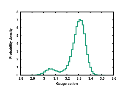
We chose a value of the gauge coupling $\beta=4.940$ that is slightly below the transition at $\mu=0$ (see Fig. 1), so that the real part of the leading Lee-Yang zeros should converge to a nonzero value in the large volume limit. We use an ensemble of 16000 configurations, each separated by 10 HMC trajectories.

Figure 2: Canonical partition functions, normalized to $Z(\hat{\mu}=0)$. Further coefficients have error bars over $100\%$, signalling the onset of the sign problem.

III.2 Calculation of the cumulants of the quark number to arbitrary order

For simplicity, we will consider the case of four flavors of quarks with degenerate quark chemical potentials $\mu_{1}=\mu_{2}=\mu_{3}=\mu_{4}\equiv\mu$. If we choose the same quantum numbers as in the 1+1+1+1 flavor physical case, i.e., if

$$\mu_{d} =\frac{1}{3}\mu_{B}-\frac{1}{3}\mu_{Q}\,,$$ (30)

$$\mu_{u} =\frac{1}{3}\mu_{B}+\frac{2}{3}\mu_{Q}\,,$$

$$\mu_{s} =\frac{1}{3}\mu_{B}-\frac{1}{3}\mu_{Q}-\mu_{S}\,,$$

$$\mu_{c} =\frac{1}{3}\mu_{B}+\frac{2}{3}\mu_{Q}-\mu_{C}\,,$$

then this choice of chemical potentials corresponds to $\mu_{B}=3\mu$, with $\mu_{Q}=\mu_{S}=\mu_{C}=0$.

Our calculation is based on the reduction formula of Ref. Hasenfratz and Toussaint (1992), which reads

$$\det M(\hat{\mu})=e^{-3V\hat{\mu}}\prod_{i=1}^{6V}\left(\xi_{i}-e^{\hat{\mu}}\right)\,,$$ (31)

where $V=N_{s}^{3}$ with $N_{s}$ the spatial linear size of the lattice, and where the $\xi_{i}$ are eigenvalues of the reduced matrix $P$ given below. Since $P$ is $\mu$-independent, once the $\xi_{i}$ are known for a given gauge configuration, one can calculate the corresponding unrooted quark determinant for arbitrary $\mu$, which allows us to extract fluctuations to arbitrarily high order on the given ensemble. Working in the temporal gauge [$U_{4}(t,\vec{x})=1$ for $0\leq t<N_{t}$], $P$ is obtained as (spatial indices are suppressed)

$$P=-\prod_{i=0}^{N_{t}-1}\begin{pmatrix}B_{i}&1\\ 1&0\end{pmatrix}L\,,$$ (32)

with $B_{i}$ the sum of the spatial derivatives and mass parts of the staggered matrix on the $i$-th time-slice, and $L$ the temporal link on the last time slice (i.e., the untraced Polyakov loop). Performing a Monte Carlo simulation at $\mu=0$, one can then obtain the partition function at nonzero $\mu$ via

$$\frac{Z(\hat{\mu})}{Z(0)} =\left\langle\frac{\det M(\hat{\mu})}{\det M(0)}\right\rangle_{0}=e^{-3V\hat{\mu}}\left\langle\prod_{i=1}^{6V}\frac{\xi_{i}-e^{\hat{\mu}}}{\xi_{i}-1}\right\rangle_{0}$$ (33)

$$=e^{-3V\hat{\mu}}\,{\cal P}(e^{\hat{\mu}})\,,$$

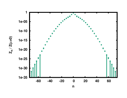
where the subscript 0 indicates that the expectation value is computed at $\mu=0$. It is evident that ${\cal P}$ is a polynomial in the fugacity, whose coefficients are the (normalized) canonical partition functions $Z_{n}/Z(0)$ [see Eq. (1)]. While here we obtain them by averaging appropriate combinations of the eigenvalues of $P$, they are usually obtained by Fourier transform from simulations at imaginary chemical potential Hasenfratz and Toussaint (1992); Morita et al. (2014); Fukuda et al. (2016); Nakamura et al. (2016); de Forcrand and Kratochvila (2006); Ejiri (2008); Li et al. (2010, 2011); Danzer and Gattringer (2012); Gattringer and Schadler (2015); Boyda et al. (2016); Goy et al. (2017); Bornyakov et al. (2017); Boyda et al. (2017); Wakayama et al. (2018); Nagata et al. (2015). Because of the Roberge-Weiss symmetry, all coefficients with $n$ not a multiple of $3$ vanish upon gauge averaging and can thus be set to zero. The normalized canonical partition functions are shown in Fig. 2.

The radius of convergence of a Taylor expansion of $\log{\cal P}$ is determined by the position of the zeros of ${\cal P}$, and it is clearly the same as that of $\log Z$, so that we can simply ignore the exponential prefactor in Eq. (33). On such a small lattice, it was possible to find all roots of $\mathcal{P}$ using standard methods. The roots can then be used, e.g., in Eq. (25) to obtain the Taylor coefficients of the expansion in the fugacity parameter $\zeta$ to arbitrarily high order. The Lee-Yang zeros closest to $\mu=0$ can be seen in Fig. 3.

Figure 3: The first five Lee-Yang zeros in the chemical potential $\hat{\mu}=\mu/T$ with their statistical errors.

Figure 4: Relative statistical error of the Taylor coefficients $c^{(\hat{\mu})}_{k}$, $c^{(\zeta)}_{k}$ and $c^{(\beta)}_{k}$ as a function of the order of the expansion. Notice that they climb to well over $100\%$.

III.3 Calculation of the cumulants of the gauge action to arbitrary order

The calculation of the coefficients $c^{(\beta)}_{k}$ is more straightforward. After a direct computation of the moments $\langle G^{n}\rangle$ one can use the following recursive formula Smith (1995),

$$\llangle G^{n}\rrangle=\langle G^{n}\rangle-\sum_{m=1}^{n-1}\binom{n-1}{m-1}\llangle G^{m}\rrangle\langle G^{n-m}\rangle\,,$$ (34)

to build all cumulants. Arbitrary precision arithmetic has to be used both in the calculation of the moments $\langle G^{n}\rangle$ and in applying the recursion formula Eq. (34). This might be somewhat counter-intuitive, as much more digits have to be kept in the calculation than the statistical error bars of the cumulants would suggest. On the other hand, the errors of the cumulants of different order are very strongly correlated, and this correlation should not be altered in order to get the radius of convergence with a reliable error estimate.

III.4 Numerical results for the convergence radius estimators

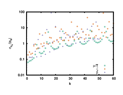
We come now to the numerical results on the convergence radius estimators mentioned in Section 2. First, we show in Fig. 4 the relative statistical error of the Taylor coefficients $c^{(\zeta)}_{k}$, $c^{(\hat{\mu})}_{k}$ and $c^{(\beta)}_{k}$. As expected, the statistical errors increase with the order of the expansion, getting to order $O(100\%)$ and above quite soon. In spite of this, as we will show below, it is possible to take combinations of them (i.e., our radius estimators) that have small error bars and give the radius of convergence directly.

Figure 5: The ratios $r^{(X)}[n]_{k}$ for several values of $n$ and $k$ in case of $X=\zeta$ (top) and $X=\hat{\mu}$ (bottom).

Figure 6: Simple ratio estimators compared to the correct radius of convergence, as given by the analysis of the Lee-Yang zeros (the light green arrow) for the case of the fugacity parameter $\zeta=e^{\hat{\mu}}-1$ (top) and the chemical potential $\hat{\mu}$ (bottom).

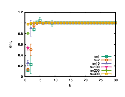
It is interesting to study how much of a particular expansion coefficient comes from the leading $n$ Lee-Yang zeros. We quantify this by the ratio

$$r^{(X)}[n]_{k}=\frac{1}{C_{k}^{(X)}}\sum_{j=1}^{n}\frac{-2}{k}\frac{\cos(k\theta_{j})}{r_{j}^{k}}\,,$$ (35)

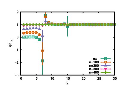
where $X$ can be either $\hat{\mu}$ or $\zeta$, the $C_{k}^{(X)}$ are given in Eq. (25), and the sum from $j=1$ to $n$ contains the $n$ Lee-Yang zeros in $\hat{\mu}^{2}$ or $\zeta$ closest to $\hat{\mu}=0$ or $\zeta=0$, limited to the upper complex half-plane. These ratios for several values of $n$ can be seen in Fig. 5.

In the case of the fugacity parameter expansion, hundreds of Lee-Yang zeros give an important contribution to low-order coefficients, before a single Lee-Yang zero starts to dominate around $k=O(10)$. For the chemical potential expansion the situation is much better, with only $O(10)$ Lee-Yang zeros contributing to the second coefficient, and the sum over zeros saturating sooner. This suggests that our estimators will work better with the chemical potential, as we shall see.

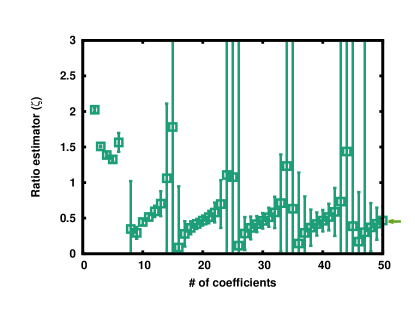
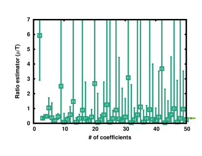
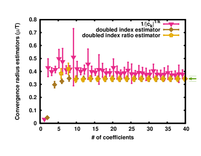
We now turn to the study of the radius of convergence. We first look at the ratio estimators, that can be seen in Fig. 6. Notice that low orders of the ratio estimator overestimate the real radius of convergence, making them very misleading. At higher orders, notice that the ratio estimator does not converge to a specific value, just as expected from our analytical discussion in Section II. Interestingly, the statistical error of the ratio estimator does get smaller when it is close to the correct value, i.e., when $\left|\frac{\cos(k\theta)}{\cos((k+1)\theta)}\right|\approx 1$. Nonetheless, it is still quite noisy there and never reaches the high statistical precision of our newly proposed estimators (see below), and based on the ratio estimator alone it would not be possible to conclude what the radius of convergence is.

In previous studies Huovinen and Petreczky (2010); Borsányi et al. (2012a); Alba et al. (2017); Huovinen and Petreczky (2018); Vovchenko et al. (2017) it was customary to compare the ratio estimators for the Taylor expansion in the baryon number chemical potential to the hadron resonance gas Dashen et al. (1969); Venugopalan and Prakash (1992). As there is no finite $\mu$ transition in this model, when such a comparison yields results consistent with the HRG one concludes that there are no signs of criticality in the fluctuations under scrutiny. In the case presented here, the HRG prediction for the first ratio is $\frac{c^{(\hat{\mu})}_{1}}{c^{(\hat{\mu})}_{2}}=\frac{1/2!}{1/4!}=6$, independently of the hadron spectrum. This matches our numerical results within error bars. The second ratio in the HRG is $\frac{c^{(\hat{\mu})}_{2}}{c^{(\hat{\mu})}_{3}}=\frac{1/4!}{1/6!}=30$. This is two orders of magnitude higher than our numerical data, so one clearly sees some sign of non-hadronic matter, but without our improved estimators it is unclear how one can make more quantitative statements.

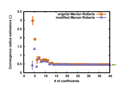
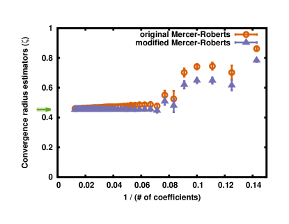
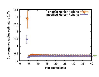
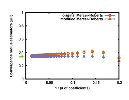
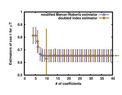
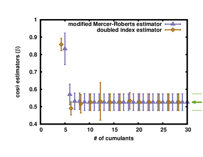
We now go on to the improved convergence radius estimators proposed in this paper. Both the original and our modified version of the Mercer-Roberts estimator can be seen for the fugacity parameter $\zeta$ in Fig. 7. As can be seen, by the time the original Mercer-Roberts estimator starts to become linear in $1/n$, so that a linear fit could be performed to obtain the convergence radius, our modified estimator already gives the correct answer. Another way to quantify the improvement achieved with our modification is to say that to get the correct convergence radius within 1$\sigma$ of the statistical error bars, our estimator needs 13 orders of the expansion, while the original Mercer-Roberts needs 20. A similar comparison for the case of the chemical potential can be seen in Fig. 8. We see that the convergence radius estimators for the chemical potential work significantly better compared to the fugacity parameter, converging to the correct value already with a 6th order (i.e., $\hat{\mu}^{12}$) expansion. Both of the Taylor series have a convergence radius determined by the leading Lee-Yang zero at $\rm{Re}\,\hat{\mu}=0.533\pm 0.020$ and $\rm{Im}\,\hat{\mu}=0.244\pm 0.016$ (Fig. 3).

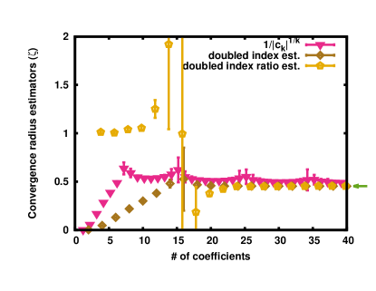
The doubled index estimator and the doubled index ratio estimator are compared to the Cauchy-Hadamard estimator for the fugacity parameter in Fig. 9 (top) and for the chemical potential in Fig. 9 (bottom). The doubled index estimator and the Cauchy-Hadamard estimator behave quite similarly qualitatively, but our proposal is a big improvement over the other, needing much fewer Taylor coefficients to approach the correct value within $1\sigma$.

Figure 7: Top: The original and our modified Mercer-Roberts estimators for the convergence radius as a function of the expansion order $n$ needed to calculate the given estimator for the variable $\zeta=e^{\hat{\mu}}-1$. Data points are slightly shifted for visual clarity. The estimators are compared to the correct radius of convergence, as given by the analysis of the Lee-Yang zeros (the light green arrow). Bottom: The same quantities, but as a function of $1/n$ for higher orders of the expansion.

Figure 8: Top: The original and our modified Mercer-Roberts estimators for the convergence radius as a function of the expansion order $n$ needed to calculate the given estimator for the variable $\hat{\mu}$. Data points are slightly shifted for visual clarity. The estimators are compared to the correct radius of convergence, as given by the analysis of the Lee-Yang zeros (the light green arrow). Bottom: The same quantities, but as a function of $1/n$ for higher orders of the expansion.

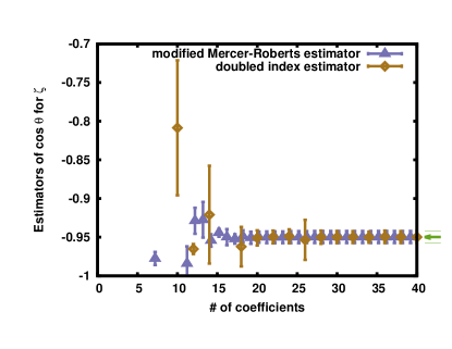
Two estimators for $\cos\theta$ can be seen in Fig. 10. For low orders in the Taylor series these estimators happen to be outside the range $[-1:1]$, which very clearly indicates that the leading Lee-Yang zeros is not dominating the series, as only in the case of a single Lee-Yang zero will these combinations reduce to a single cosine.

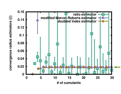
Finally, let us turn to the analysis of the Fisher zeros. In this case we do not calculate the cumulants starting from the partition function zeros, and therefore the large cancellations of the errors, coming from the correlations between the different cumulants, can be directly demonstrated. This is shown in Fig. 11, where we show some estimators for the radius and for the cosine of the phase, and compare them to results obtained by reweighting to complex $\beta$. We can see that the ratio estimator again does not work, while our newly proposed estimators work well, and give error bars identical to those obtained with reweighting.

IV Summary and outlook

Figure 9: The Cauchy-Hadamard estimator and our doubled index and doubled index ratio estimators for $\zeta$ (top) and $\hat{\mu}$ (bottom). Data points are slightly shifted for visual clarity. The estimators are compared to the correct radius of convergence, as given by the analysis of the Lee-Yang zeros (the light green arrow).

Figure 10: Estimators of $\cos\theta$ built from the doubled index and modified Mercer-Roberts estimators for $\zeta$ (top) and $\hat{\mu}$ (bottom). Data points are slightly shifted for visual clarity. The estimators are compared to the correct radius of convergence, as given by the analysis of the Lee-Yang zeros (the light green arrow). For low orders (not shown in the plot) certain estimators give values outside the plot range.

In studies of QCD at finite chemical potential, it is a standard approach to try to infer the position of the critical endpoint from the radius of convergence of the Taylor expansion of the pressure, either in the chemical potential over temperature, $\hat{\mu}$, or in the fugacity parameter $\zeta=e^{\hat{\mu}}-1$. In this paper we have demonstrated, on general grounds, that the simple ratio estimator cannot work if one wants to determine the radius of convergence in a finite volume first, and take the thermodynamic limit afterwards, and has serious drawbacks even if the radius of convergence is computed directly in the thermodynamic limit. This follows from the analytic structure of the grand canonical QCD partition function in a finite volume.

The analytic structure of the partition function is also the starting point for the construction of three new convergence radius estimators, that are designed precisely to work well in a finite volume, where they determine the distance from the origin of the closest Lee-Yang zero. We also constructed estimators for the cosine of the phase of the leading Lee-Yang zero. In this way we are able, at least in principle, to locate the leading Lee-Yang zero in the complex $\hat{\mu}$ or $\zeta$ plane. On a conceptual level, this provides a link between the reweighting and Taylor expansion methods, demonstrating how to obtain the leading Lee-Yang zero from the Taylor expansion, which was a quantity that was traditionally obtained by reweighting in the literature.

Since the expansion order that can be reached is in practice limited, and it is not known a priori how fast the estimators converge to their asymptotic value, having different estimators at one’s disposal allows to cross-check whether for the highest accessible expansion order the Taylor series is already dominated by a single Lee-Yang zero or not. Interestingly, the relative statistical error of our estimators at high enough order is expected to converge to a finite value, contrary to what happens to the error of the expansion coefficients themselves. This allows in principle to give a reliable estimate of the correct location of the leading Lee-Yang zero. In particular, our derivation makes it clear that for any given ensemble, if one uses our improved estimators, the study of the Taylor coefficients and the direct determination of the Lee-Yang zeros via reweighting should give identical results.

In order to test our proposals, we have performed an exploratory study with $N_{f}=4$ unimproved staggered fermions on a small $6^{3}\times 4$ volume, with bare quark mass chosen in order to have a first-order phase transition (in the large-volume limit at fixed temporal extent in lattice units), and for a temperature in the chirally-broken phase close to the transition. For such a small system it is possible to determine all the Lee-Yang zeros by standard methods, and thus to obtain explicitly the radius of convergence and all the Taylor coefficients. Our estimators work well, as expected, achieving a rather accurate determination of the radius of convergence with $O(15)$ Taylor coefficients in the case of $\zeta$, and only around 6 coefficients in the case of $\hat{\mu}$. This is not far from the situation currently available for realistic lattices, i.e., lattices near the continuum limit of $N_{f}=2+1$ flavor QCD with physical masses, where currently we have coefficients at most up to $c_{4}$, corresponding to $\chi_{8}$ in the usual notation for the Taylor series in QCD, or $b_{4}$ with the notation of Vovchenko et al. (2017), which refers to the Fourier series in imaginary chemical potential. While the number of Taylor coefficients needed for an accurate determination of the radius of convergence with our estimators is most certainly model dependent, and therefore could be larger for realistic lattices, nevertheless one can hope that it still remains reasonable. At the same time, there is no reason to expect the situation to get better for the ratio estimator, meaning that the existing results of the first few orders of the ratio estimator D’Elia et al. (2017); Bazavov et al. (2017); Fodor et al. (2018) are likely not that informative about the true radius of convergence.

A particularly encouraging aspect of our study is the statistical accuracy of our estimators, which is vastly better than that of the coefficients themselves. This can be explained by noticing that the statistical errors on the coefficients are strongly correlated, which leads to cancellations when they are combined into our convergence radius estimators.

We have also demonstrated our method on Fisher zeros. While this is phenomenologically less interesting, it demonstrates explicitly the big cancellations of errors that we expect from our picture. In fact, the results obtained with our new estimators are consistent with, and have the same relative precision as those obtained independently via reweighting from the same ensemble.

There is a somewhat uplifting message to all this. While in our exploratory study we find over $100\%$ error bars on most of the coefficients, it nevertheless turns out that with an ensemble of reasonable size it is possible to determine the position of the leading Lee-Yang zero quite accurately. In other words, the errors on the Taylor coefficient do not reflect the actual uncertainty with which the leading Lee-Yang zero can be obtained. It might then even be possible to extract the position of the leading Lee-Yang zero already from existing ensembles, just not with the method currently pursued in the literature (i.e., ratio estimators from Taylor expansion coefficients). Determining an efficient method for this is an important task for the future.

Figure 11: Top: The ratio, modified Mercer-Roberts and doubled index estimators for the distance of the leading pair of Fisher zeros, compared to the result obtained from reweighting (the light green arrow). Data points are slightly shifted for visual clarity. Bottom: The modified Mercer-Roberts and doubled index estimators for the phase.

References

- Hasenfratz and Toussaint (1992) A. Hasenfratz and D. Toussaint, Nucl. Phys. B371, 539 (1992).
- Barbour et al. (1998) I. M. Barbour, S. E. Morrison, E. G. Klepfish, J. B. Kogut, and M. P. Lombardo, Lattice QCD on parallel computers. Proceedings, International Workshop, Tsukuba, Japan, March 10-15, 1997, Nucl. Phys. Proc. Suppl. 60A, 220 (1998), [,220(1997)], arXiv:hep-lat/9705042 [hep-lat] .
- Fodor and Katz (2002a) Z. Fodor and S. D. Katz, Phys. Lett. B534, 87 (2002a), arXiv:hep-lat/0104001 [hep-lat] .
- Fodor and Katz (2002b) Z. Fodor and S. D. Katz, JHEP 03, 014, arXiv:hep-lat/0106002 [hep-lat] .
- Fodor and Katz (2004) Z. Fodor and S. D. Katz, JHEP 04, 050, arXiv:hep-lat/0402006 [hep-lat] .
- Csikor et al. (2004) F. Csikor, G. I. Egri, Z. Fodor, S. D. Katz, K. K. Szabó, and A. I. Tóth, JHEP 05, 046, arXiv:hep-lat/0401016 [hep-lat] .
- Allton et al. (2002) C. R. Allton, S. Ejiri, S. J. Hands, O. Kaczmarek, F. Karsch, E. Laermann, C. Schmidt, and L. Scorzato, Phys. Rev. D66, 074507 (2002), arXiv:hep-lat/0204010 [hep-lat] .
- Allton et al. (2005) C. R. Allton, M. Doring, S. Ejiri, S. J. Hands, O. Kaczmarek, F. Karsch, E. Laermann, and K. Redlich, Phys. Rev. D71, 054508 (2005), arXiv:hep-lat/0501030 [hep-lat] .
- Gavai and Gupta (2008) R. V. Gavai and S. Gupta, Phys. Rev. D78, 114503 (2008), arXiv:0806.2233 [hep-lat] .
- Basak et al. (2008) S. Basak et al. (MILC), Proceedings, 26th International Symposium on Lattice field theory (Lattice 2008): Williamsburg, USA, July 14-19, 2008, PoS LATTICE2008, 171 (2008), arXiv:0910.0276 [hep-lat] .
- Borsányi et al. (2012a) S. Borsányi, Z. Fodor, S. D. Katz, S. Krieg, C. Ratti, and K. Szabó, JHEP 01, 138, arXiv:1112.4416 [hep-lat] .
- Borsányi et al. (2012b) S. Borsányi, G. Endrődi, Z. Fodor, S. Katz, S. Krieg, et al., JHEP 1208, 053, arXiv:1204.6710 [hep-lat] .
- Bellwied et al. (2015) R. Bellwied, S. Borsányi, Z. Fodor, J. Günther, S. D. Katz, C. Ratti, and K. K. Szabó, Phys. Lett. B751, 559 (2015), arXiv:1507.07510 [hep-lat] .
- Ding et al. (2015) H. T. Ding, S. Mukherjee, H. Ohno, P. Petreczky, and H. P. Schadler, Phys. Rev. D92, 074043 (2015), arXiv:1507.06637 [hep-lat] .
- Bazavov et al. (2017) A. Bazavov et al., Phys. Rev. D95, 054504 (2017), arXiv:1701.04325 [hep-lat] .
- de Forcrand and Philipsen (2002) P. de Forcrand and O. Philipsen, Nucl. Phys. B642, 290 (2002), arXiv:hep-lat/0205016 [hep-lat] .
- D’Elia and Lombardo (2003) M. D’Elia and M. P. Lombardo, Phys. Rev. D67, 014505 (2003), arXiv:hep-lat/0209146 [hep-lat] .
- D’Elia and Sanfilippo (2009) M. D’Elia and F. Sanfilippo, Phys. Rev. D80, 014502 (2009), arXiv:0904.1400 [hep-lat] .
- Bonati et al. (2014) C. Bonati, P. de Forcrand, M. D’Elia, O. Philipsen, and F. Sanfilippo, Phys. Rev. D90, 074030 (2014), arXiv:1408.5086 [hep-lat] .
- Bonati et al. (2015) C. Bonati, M. D’Elia, M. Mariti, M. Mesiti, F. Negro, and F. Sanfilippo, Phys. Rev. D92, 054503 (2015), arXiv:1507.03571 [hep-lat] .
- D’Elia et al. (2017) M. D’Elia, G. Gagliardi, and F. Sanfilippo, Phys. Rev. D95, 094503 (2017), arXiv:1611.08285 [hep-lat] .
- Günther et al. (2017) J. N. Günther, R. Bellwied, S. Borsányi, Z. Fodor, S. D. Katz, A. Pásztor, C. Ratti, and K. K. Szabó, Proceedings, 26th International Conference on Ultra-relativistic Nucleus-Nucleus Collisions (Quark Matter 2017): Chicago, Illinois, USA, February 5-11, 2017, Nucl. Phys. A967, 720 (2017), arXiv:1607.02493 [hep-lat] .
- Vovchenko et al. (2017) V. Vovchenko, A. Pásztor, Z. Fodor, S. D. Katz, and H. Stoecker, Phys. Lett. B775, 71 (2017), arXiv:1708.02852 [hep-ph] .
- Bonati et al. (2018) C. Bonati, M. D’Elia, F. Negro, F. Sanfilippo, and K. Zambello, Phys. Rev. D98, 054510 (2018), arXiv:1805.02960 [hep-lat] .
- Borsányi et al. (2018) S. Borsányi, Z. Fodor, J. N. Günther, S. K. Katz, K. K. Szabó, A. Pásztor, I. Portillo, and C. Ratti, JHEP 10, 205, arXiv:1805.04445 [hep-lat] .
- Fodor et al. (2018) Z. Fodor, M. Giordano, J. N. Günther, K. Kapás, S. D. Katz, A. Pásztor, I. Portillo, C. Ratti, D. Sexty, and K. K. Szabó, in 27th International Conference on Ultrarelativistic Nucleus-Nucleus Collisions (Quark Matter 2018) Venice, Italy, May 14-19, 2018 (2018) arXiv:1807.09862 [hep-lat] .
- Lee and Yang (1952) T. D. Lee and C.-N. Yang, Phys. Rev. 87, 410 (1952), [,157(1952)].
- Rudin (1997) W. Rudin, Real and complex analysis, 3rd ed. (McGraw-Hill, 1997).
- Roberge and Weiss (1986) A. Roberge and N. Weiss, Nucl. Phys. B275, 734 (1986).
- Skokov et al. (2011) V. Skokov, K. Morita, and B. Friman, Phys. Rev. D83, 071502 (2011), arXiv:1008.4549 [hep-ph] .
- Flindt and Garrahan (2013) C. Flindt and J. P. Garrahan, Phys. Rev. Lett. 110, 050601 (2013).
- Brandner et al. (2017) K. Brandner, V. F. Maisi, J. P. Pekola, J. P. Garrahan, and C. Flindt, Phys. Rev. Lett. 118, 180601 (2017).
- Deger et al. (2018) A. Deger, K. Brandner, and C. Flindt, Phys. Rev. E 97, 012115 (2018).
- Ahlfors (1979) L. V. Ahlfors, Complex analysis, 3rd ed. (McGraw-Hill, 1979).
- Mercer and Roberts (1990) G. N. Mercer and A. J. Roberts, SIAM Journal on Applied Mathematics 50, 1547 (1990).
- Kogut et al. (1987) J. B. Kogut, H. W. Wyld, F. Karsch, and D. K. Sinclair, Phys. Lett. B188, 353 (1987).
- Morita et al. (2014) K. Morita, V. Skokov, B. Friman, and K. Redlich, Eur. Phys. J. C74, 2706 (2014), arXiv:1211.4703 [hep-ph] .
- Fukuda et al. (2016) R. Fukuda, A. Nakamura, and S. Oka, Phys. Rev. D93, 094508 (2016), arXiv:1504.06351 [hep-lat] .
- Nakamura et al. (2016) A. Nakamura, S. Oka, and Y. Taniguchi, JHEP 02, 054, arXiv:1504.04471 [hep-lat] .
- de Forcrand and Kratochvila (2006) P. de Forcrand and S. Kratochvila, Hadron physics, proceedings of the Workshop on Computational Hadron Physics, University of Cyprus, Nicosia, Cyprus, 14-17 September 2005, Nucl. Phys. Proc. Suppl. 153, 62 (2006), [,62(2006)], arXiv:hep-lat/0602024 [hep-lat] .
- Ejiri (2008) S. Ejiri, Phys. Rev. D78, 074507 (2008), arXiv:0804.3227 [hep-lat] .
- Li et al. (2010) A. Li, A. Alexandru, K.-F. Liu, and X. Meng, Phys. Rev. D82, 054502 (2010), arXiv:1005.4158 [hep-lat] .
- Li et al. (2011) A. Li, A. Alexandru, and K.-F. Liu, Phys. Rev. D84, 071503 (2011), arXiv:1103.3045 [hep-ph] .
- Danzer and Gattringer (2012) J. Danzer and C. Gattringer, Phys. Rev. D86, 014502 (2012), arXiv:1204.1020 [hep-lat] .
- Gattringer and Schadler (2015) C. Gattringer and H.-P. Schadler, Phys. Rev. D91, 074511 (2015), arXiv:1411.5133 [hep-lat] .
- Boyda et al. (2016) D. L. Boyda, V. G. Bornyakov, V. A. Goy, V. I. Zakharov, A. V. Molochkov, A. Nakamura, and A. A. Nikolaev, JETP Lett. 104, 657 (2016), [Pisma Zh. Eksp. Teor. Fiz.104,no.10,673(2016)].
- Goy et al. (2017) V. A. Goy, V. Bornyakov, D. Boyda, A. Molochkov, A. Nakamura, A. Nikolaev, and V. Zakharov, PTEP 2017, 031D01 (2017), arXiv:1611.08093 [hep-lat] .
- Bornyakov et al. (2017) V. G. Bornyakov, D. L. Boyda, V. A. Goy, A. V. Molochkov, A. Nakamura, A. A. Nikolaev, and V. I. Zakharov, Phys. Rev. D95, 094506 (2017), arXiv:1611.04229 [hep-lat] .
- Boyda et al. (2017) D. Boyda, V. G. Bornyakov, V. Goy, A. Molochkov, A. Nakamura, A. Nikolaev, and V. I. Zakharov, (2017), arXiv:1704.03980 [hep-lat] .
- Wakayama et al. (2018) M. Wakayama, V. G. Borynakov, D. L. Boyda, V. A. Goy, H. Iida, A. V. Molochkov, A. Nakamura, and V. I. Zakharov, (2018), arXiv:1802.02014 [hep-lat] .
- Nagata et al. (2015) K. Nagata, K. Kashiwa, A. Nakamura, and S. M. Nishigaki, Phys. Rev. D91, 094507 (2015), arXiv:1410.0783 [hep-lat] .
- Smith (1995) P. J. Smith, Am. Stat. 49, 217 (1995).
- Huovinen and Petreczky (2010) P. Huovinen and P. Petreczky, Nucl. Phys. A837, 26 (2010), arXiv:0912.2541 [hep-ph] .
- Alba et al. (2017) P. Alba et al., Phys. Rev. D96, 034517 (2017), arXiv:1702.01113 [hep-lat] .
- Huovinen and Petreczky (2018) P. Huovinen and P. Petreczky, Phys. Lett. B777, 125 (2018), arXiv:1708.00879 [hep-ph] .
- Dashen et al. (1969) R. Dashen, S.-K. Ma, and H. J. Bernstein, Phys. Rev. 187, 345 (1969).
- Venugopalan and Prakash (1992) R. Venugopalan and M. Prakash, Nucl. Phys. A546, 718 (1992).