![[Uncaptioned image]](/html/1904.00018/assets/x1.png)
Nikhef/2019-005
Nuclear Parton Distributions from Lepton-Nucleus Scattering
and the Impact of an Electron-Ion Collider
The NNPDF Collaboration:
Rabah Abdul Khalek, Jacob J. Ethier, and Juan Rojo
Department of Physics and Astronomy, Vrije Universiteit
Amsterdam, 1081 HV
Amsterdam,
Nikhef Theory Group, Science Park 105, 1098 XG Amsterdam, The
Netherlands.
Abstract
We present a first determination of the nuclear parton distribution functions (nPDF) based on the NNPDF methodology: nNNPDF1.0. This analysis is based on neutral-current deep-inelastic structure function data and is performed up to NNLO in QCD calculations with heavy quark mass effects. For the first time in the NNPDF fits, the minimization is achieved using stochastic gradient descent with reverse-mode automatic differentiation (backpropagation). We validate the robustness of the fitting methodology through closure tests, assess the perturbative stability of the resulting nPDFs, and compare them with other recent analyses. The nNNPDF1.0 distributions satisfy the boundary condition whereby the NNPDF3.1 proton PDF central values and uncertainties are reproduced at , which introduces important constraints particularly for low- nuclei. We also investigate the information that would be provided by an Electron-Ion Collider (EIC), finding that EIC measurements would significantly constrain the nPDFs down to . Our results represent the first-ever nPDF determination obtained using a Monte Carlo methodology consistent with that of state-of-the-art proton PDF fits, and provide the foundation for a subsequent global nPDF analyses including also proton-nucleus data.
1 Introduction
It has been known for more than three decades [1] that the parton distribution functions (PDFs) of nucleons bound within nuclei, more simply referred to as nuclear PDFs (nPDFs) [2, 3], can be modified with respect to their free-nucleon counterparts [4]. Since MeV-scale nuclear binding effects were expected to be negligible compared to the typical momentum transfers ( GeV) in hard-scattering reactions such as deep-inelastic lepton-nucleus scattering, such a phenomena came as a surprise to many in the physics community. Despite active experimental and theoretical investigations, the underlying mechanisms that drive in-medium modifications of nucleon substructure are yet to be fully understood. The determination of nPDFs is therefore relevant to improve our fundamental understanding of the strong interactions in the nuclear environment.
In addition to pinning down the dynamics of QCD in heavy nuclei, nPDFs are an essential ingredient for the interpretation of heavy ion collisions at RHIC and the LHC, in particular for the characterization of the Quark-Gluon Plasma (QGP) [5, 6] via hard probes. Moreover, a reliable determination of the nuclear PDFs is required to separate the hot nuclear matter (QGP) from the cold nuclear matter effects that will in general already be present in the initial stages of the heavy ion collision.
The importance of nPDF fits is further highlighted by their contribution to the quark flavor separation in global PDF analyses of the proton [7, 8, 9, 10]. Even with constraints from related processes such as gauge boson production at the Tevatron and the LHC, information provided by neutrino-induced charged current deep-inelastic scattering on heavy nuclear targets play a critical role in disentangling the proton’s quark and antiquark distributions. However, given the current precision of proton PDF fits, neglecting the nuclear uncertainties associated with neutrino-nucleus scattering may not be well justified anymore [11], as opposed to the situation some years ago [12].
Lastly, nPDF extractions can sharpen the physics case of future high-energy lepton-nucleus colliders such as the Electron-Ion Collider (EIC) [13] and the Large Hadron electron Collider (LHeC) [14, 15], which will probe nuclear structure deep in the region of small parton momentum fractions, , and aim to unravel novel QCD dynamics such as non-linear (saturation) effects. The latter will only be possible provided that a faithful estimate of the nPDF uncertainties at small can be attained, similar to what was required for the recent discovery of BFKL dynamics from the HERA structure function data [16].
Unfortunately, the determination of the nuclear PDFs is hampered by the rather limited experimental dataset available. In fact, until a few years ago, most nPDF analyses [17, 18, 19, 20, 21, 22] were largely based on fixed-target DIS structure functions in lepton-nucleus scattering (with kinematic coverage restricted to ) supplemented by some Drell-Yan cross-sections. A major improvement in this respect has been the recent availability of data on hard-scattering cross-sections from proton-lead collisions at the LHC, with processes ranging from jet [23, 24, 25, 26, 27] and electroweak boson production [28, 29, 30, 31, 32], to heavy quark production [33, 34, 35, 36, 37, 38, 39, 40] among several others. Indeed, measurements of hard probes in p+Pb collisions provide useful information to constrain the nPDFs, as was demonstrated by a few recent studies [41, 42].
On the other hand, a survey of various nPDF determinations reveals limitations that are of methodological origin as well. First of all, current nuclear PDF fits rely on model-dependent assumptions for the parameterization of the non-perturbative and atomic mass number dependence, resulting in a theoretical bias whose magnitude is difficult to assess. Moreover, several nPDF sets are extracted in terms of a proton baseline (to which the former must reduce in the limit) that have been determined by other groups based on fitting methodologies and theoretical settings which might not fully equivalent, for instance, in the prescriptions used to estimate the nPDF uncertainties. Finally, PDF uncertainties are often estimated using the Hessian method, which is restricted to a Gaussian approximation with ad hoc tolerances, introducing a level of arbitrariness in their statistical interpretation.
Motivated by this need for a reliable and consistent determination of nuclear PDFs and their uncertainties, we present in this work a first nPDF analysis based on the NNPDF methodology [43, 44, 45, 46, 47, 48, 49, 50, 51, 52]: nNNPDF1.0. In this initial study, we restrict our analysis to neutral-current nuclear deep-inelastic structure function measurements, and compute the corresponding predictions in QCD up to NNLO in the expansion. Moreover, heavy quark mass effects are included using the FONLL general-mass variable-flavor number scheme [53]. Since the nPDFs are determined using the same theoretical and methodological framework as the NNPDF3.1 proton PDFs, we are able to impose the boundary condition in a consistent manner so that the nNNPDF1.0 results reproduce both the NNPDF3.1 central values and uncertainties when evaluated at .
The nNNPDF1.0 sets are constructed following the general fitting methodology outlined in previous NNPDF studies, which utilizes robust Monte Carlo techniques to obtain a faithful estimate of nPDF uncertainties. In addition, in this study we implement for the first time stochastic gradient descent to optimize the model parameters. This is performed using TensorFlow [54], an open source machine learning library in which the gradients of the function can be computed via automatic differentiation. Together with several other improvements, we present a validation of the nNNPDF1.0 methodology through closure tests.
As a first phenomenological application of the nNNPDF1.0 sets, we quantify the impact of future lepton-nucleus scattering measurements provided by an Electron-Ion Collider. Using pseudo-data generated with different electron and nucleus beam energy configurations, we perform fits to quantify the effect on the nNNPDF1.0 uncertainties and discuss the extent to which novel QCD dynamics can be revealed. More specifically, we demonstrate how the EIC would lead to a significant reduction of the nPDF uncertainties at small , paving the way for a detailed study of nuclear matter in a presently unexplored kinematic region.
The outline of this paper is the following. In Sect. 2 we present the input experimental data used in this analysis, namely ratios of neutral-current deep-inelastic structure functions, followed by a discussion of the corresponding theoretical calculations. The description of the fitting strategy, including the updated minimization procedure and choice of parameterization, is presented in Sect. 3. We discuss the validation of our fitting methodology via closure tests in Sect. 4. The main results of this work, the nNNPDF1.0 nuclear parton distributions, are then presented in Sect. 5. In Sect. 6 we quantify the impact on the nPDFs from future EIC measurements of nuclear structure functions. Lastly, in Sect. 7 we summarize and discuss the outlook for future studies.
2 Experimental data and theory calculations
In this section we review the formalism that describes deep-inelastic scattering (DIS) of charged leptons off of nuclear targets. We then present the data sets that have been used in the present determination of the nuclear PDFs, discussing also the kinematical cuts and the treatment of experimental uncertainties. Lastly, we discuss the theoretical framework for the evaluation of the DIS structure functions, including the quark and anti-quark flavor decomposition, the heavy quark mass effects, and the software tools used for the numerical calculations.
2.1 Deep-inelastic lepton-nucleus scattering
The description of hard-scattering collisions involving nuclear targets begins with collinear factorization theorems in QCD that are identical to those in free-nucleon scattering.
For instance, in deep inelastic lepton-nucleus scattering, the leading power contribution to the cross section can be expressed in terms of a hard partonic cross section that is unchanged with respect to the corresponding lepton-nucleon reaction, and the nonperturbative PDFs of the nucleus. Since these nPDFs are defined by the same leading twist operators as the free nucleon PDFs but acting instead on nuclear states, the modifications from internal nuclear effects are naturally contained within the nPDF definition and the factorization theorems remain valid assuming power suppressed corrections are negligible in the perturbative regime, 1 GeV2. We note, however, that this assumption may not hold for some nuclear processes, and therefore must be studied and verified through the analysis of relevant physical observables.
We start now by briefly reviewing the definition of the DIS structure functions and of the associated kinematic variables which are relevant for the description of lepton-nucleus scattering. The double differential cross-section for scattering of a charged lepton off a nucleus with atomic mass number is given by
| (2.1) |
where and the usual DIS kinematic variables can be expressed in Lorentz-invariant form as
| (2.2) |
Here the four-momenta of the target nucleon, the incoming charged lepton, and the exchanged virtual boson ( or ) are denoted by , , and , respectively. The variable is defined here to be the standard Bjorken scaling variable, which at leading order can be interpreted as the fraction of the nucleon’s momentum carried by the struck parton, and is known as the inelasticity. Lastly, the virtuality of the exchanged boson is , which represents the hardness of the scattering reaction.
As will be discussed below, the maximum value of the momentum transfer in the nNNPDF1.0 input dataset is GeV2 (see Fig. 2.1). Given that , the contribution from the parity-violating structure functions and the contributions to and arising from boson exchange can be safely neglected. Therefore, for the kinematic range relevant to the description of available nuclear DIS data, Eq. (2.1) simplifies to
| (2.3) |
where only the photon-exchange contributions are retained for the and structure functions. In Eq. (2.3) we have isolated the dominant dependence, since the second term is typically rather small. Note that since the center of mass energy of the lepton-nucleon collision is determined by
| (2.4) |
where hadron and lepton masses have been neglected, measurements with the same values for and but different center of mass energies will lead to a different value of the prefactor in front of the ratio in Eq. (2.3), allowing in principle the separation of the two structure functions as in the free proton case.
2.2 Experimental data
In this analysis, we include all available inclusive DIS measurements of neutral-current structure functions on nuclear targets. In particular, we use data from the EMC [55, 56, 57, 58], NMC [59, 60, 61, 62], and BCDMS experiments at CERN, E139 measurements from SLAC [63], and E665 data from Fermilab. The measurements of nuclear structure functions are typically presented as ratios of the form
| (2.5) |
where and are the atomic mass numbers of the two different nuclei. Some of the experimental measurements included in this analysis are presented instead as ratios of DIS cross-sections. As discussed earlier, the double-differential DIS cross-sections are related to the and structure functions by
| (2.6) |
Therefore, one should in principle account for the contributions from the longitudinal structure function to cross-section ratios measured by experiment. However, it is well known that the ratio exhibits a very weak dependence with [64, 65], and therefore the second term in Eq. (2.6) cancels out to a good approximation when taking ratios between different nuclei. In other words, we can exploit the fact that
| (2.7) |
in which then the ratios of DIS cross-sections for in the form of Eq. (2.6) are equivalent to ratios of the structure functions. Lastly, it is important to note that whenever the nuclei involved in the measurements are not isoscalar, the data is corrected to give isoscalar ratios and an additional source of systematic error is added as a result of this conversion.
Summarized in Table 2.1 are the different types of nuclei measured by the experiments included in the nNNPDF1.0 analysis. For each dataset, we indicate the nuclei and that are used to construct the structure function ratios in Eq. 2.5, quoting explicitly the corresponding atomic mass numbers. We also display the number of data points that survive the baseline kinematical cuts, and give the corresponding publication references.
| Experiment | Reference | ||
|---|---|---|---|
| SLAC E-139 | 4He/2D | 3 | [66] |
| NMC 95, re. | 4He/2D | 13 | [59] |
| NMC 95 | 6Li/2D | 12 | [60] |
| SLAC E-139 | 9Be/2D | 3 | [66] |
| NMC 96 | 9Be/12C | 14 | [61] |
| EMC 88, EMC 90 | 12C/2D | 12 | [56, 57] |
| SLAC E-139 | 12C/2D | 2 | [66] |
| NMC 95, NMC 95, re. | 12C/2D | 26 | [60, 59] |
| FNAL E665 | 12C/2D | 3 | [67] |
| NMC 95, re. | 12C/6Li | 9 | [59] |
| BCDMS 85 | 14N/2D | 9 | [68] |
| SLAC E-139 | 27Al/2D | 3 | [66] |
| NMC 96 | 27Al/12C | 14 | [61] |
| SLAC E-139 | 40Ca/2D | 2 | [66] |
| NMC 95, re. | 40Ca/2D | 12 | [59] |
| EMC 90 | 40Ca/2D | 3 | [57] |
| FNAL E665 | 40Ca/2D | 3 | [67] |
| NMC 95, re. | 40Ca/6Li | 9 | [59] |
| NMC 96 | 40Ca/12C | 23 | [61] |
| EMC 87 | 56Fe/2D | 58 | [55] |
| SLAC E-139 | 56Fe/2D | 8 | [66] |
| NMC 96 | 56Fe/12C | 14 | [61] |
| BCDMS 85, BCDMS 87 | 56Fe/2D | 16 | [68, 69] |
| EMC 88, EMC 93 | 64Cu/2D | 27 | [56, 58] |
| SLAC E-139 | 108Ag/2D | 2 | [66] |
| EMC 88 | 119Sn/2D | 8 | [56] |
| NMC 96, dependence | 119Sn/12C | 119 | [62] |
| FNAL E665 | 131Xe/2D | 4 | [70] |
| SLAC E-139 | 197Au/2D | 3 | [66] |
| FNAL E665 | 208Pb/2D | 3 | [67] |
| NMC 96 | 208Pb/12C | 14 | [61] |
| Total | 451 |
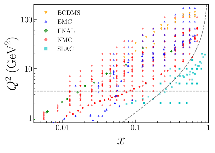
In Fig. 2.1 we show the kinematical coverage in the plane of the DIS nuclear data included in nNNPDF1.0. To minimize the contamination from low-scale non-perturbative corrections and higher-twist effects, and also to remain consistent with the baseline proton PDF analysis (to be discussed in Sect. 3), we impose the same kinematical cuts on and the invariant final state mass squared as in the NNPDF3.1 global fit [71], namely
| (2.8) |
which are represented by the dashed lines in Fig. 2.1. In Table 2.2, we compare our kinematics cuts in and to those implemented in the nCTEQ15 and EPPS16 fits. We find that our cuts are very similar to those of the nCTEQ15 analysis [20], and as a result our neutral-current DIS nuclear structure function dataset is similar to that used in their analysis. On the other hand, our choice of both the and cut is more stringent than that made in the EPPS16 analysis [41], where they set GeV2 and do not impose any cut in .
| nNNPDF1.0 | nCTEQ15 | EPPS16 | |
|---|---|---|---|
| 12.5 GeV2 | 12.25 GeV2 | n/a | |
| 3.5 GeV2 | 4 GeV2 | 1.69 GeV2 |
After imposing the kinematical cuts in Eq. (2.8), we end up with data points. As indicated in Table 2.1, around half of these points correspond to ratios of heavy nuclei with respect to to deuterium, namely in the notation of Eq. (2.5). For the rest of the data points, the values of and both correspond to heavier nuclei, with . It is worth noting that the measurements from the NMC collaboration contain a significant amount of points for which the carbon structure function is in the denominator, . In particular, we have data points for the dependence of the tin to carbon ratio, . These measurements provide valuable constraints on the dependence of the nuclear PDFs, since nuclear effects enter both the numerator and denominator of Eq. (2.5).
Concerning the treatment of the experimental uncertainties, we account for all correlations among data points whenever this information is provided by the corresponding experiments. This information is then encoded into the experimental covariance matrix, constructed using the prescription [48]:
| (2.9) | |||||
where one treats the additive (‘sys,a’) relative experimental systematic errors separately from the multiplicative (‘sys,m’) ones. In the additive case, the central value of the experimental measurement is used for the structure function ratio, . In the multiplicative case, e.g. for overall normalization uncertainties, a fixed set of theoretical predictions for the ratios, , is constructed. These predictions are typically obtained from a previous fit which is then iterated until convergence is reached. The use of the covariance matrix defined in Eq. (2.9) for the minimization (to be discussed in Sect. 3) avoids the bias associated with multiplicative uncertainties, which lead to a systematic underestimation of the best-fit values compared to their true values [72].
For the case in which correlated systematic uncertainties are not available, we simply add statistical and systematic errors in quadrature and Eq. (2.9) reduces to
| (2.10) |
where . It turns out that for all of the measurements listed in Table 2.1, the detailed break-up of the experimental systematic errors is not available (in most cases these partially or totally cancel out when taking ratios of observables), and the only systematic error that enters the covariance matrix Eq. (2.9) is the multiplicative normalization error.
2.3 Numerical implementation
We turn now to discuss the numerical implementation of the calculations of the DIS structure functions and their ratios relevant for the nPDF interpretation of the nuclear DIS data. In the framework of collinear QCD factorization, the structure function can be decomposed in terms of hard-scattering coefficient functions and nuclear PDFs as,
| (2.11) |
where are the process-dependent coefficient functions which can be computed perturbatively as an expansion in the QCD and QED couplings; is an evolution operator, determined by the solutions of the DGLAP equations, which evolves the nPDF from the initial parameterization scale into the hard-scattering scale , are the nPDFs at the parameterization scale, and denotes the Mellin convolution. The sum over flavors runs over the active quarks and antiquarks flavors at a given scale , as well as over the gluon.
The direct calculation of Eq. (2.3) during the nPDF fit is not practical since it requires first solving the DGLAP evolution equation for each new boundary condition at and then convoluting with the coefficient functions. To evaluate Eq. (2.3) in a more computationally efficient way, it is better to precompute all the perturbative information, i.e. the coefficient functions and the evolution operators , with a suitable interpolation basis. Several of these approaches have been made available in the context of PDF fits [73, 74, 75, 76]. Here we use the APFELgrid tool [77] to precompute the perturbative information of the nDIS structure functions provided by the APFEL program [78].
Within this approach, we can factorize the dependence on the nPDFs at the input scale from the rest of Eq. (2.3) as follows. First, we introduce an expansion over a set of interpolating functions spanning both and such that
| (2.12) |
where the nPDFs are now tabulated in a grid in the plane, . We can express this result in terms of the PDFs at the input evolution scale using the (interpolated) DGLAP evolution operators,
| (2.13) |
so that the nuclear DIS structure function can be evaluated as
| (2.14) |
This can be rearranged to give
| (2.15) |
where all of the information about the partonic cross-sections and the DGLAP evolution operators is now encoded into the so-called FK table, . Therefore, with the APFELgrid method we are able to express the series of convolutions in Eq.(2.3) by a matrix multiplication in Eq. (2.15), increasing the numerical calculation speed of the DIS structure functions by up to several orders of magnitude.
In this work, the FK tables (and thus the nDIS structure functions) are computed up to NNLO in the QCD coupling expansion, with heavy quark effects evaluated by the FONLL general-mass variable flavor number scheme [53]. Specifically, we use the FONLL-B scheme for the NLO fits and the FONLL-C for the NNLO fits. The value of the strong coupling constant is set to be , consistent with the PDG average [79] and with recent high-precision determinations [80, 81, 82, 83] (see [84] for an overview). Our variable flavor number scheme has a maximum of active quarks, where the heavy quark pole masses are taken to be GeV and GeV following the Higgs Cross-Sections Working Group recommendations [85]. The charm and bottom PDFs are generated dynamically from the gluon and the light quark PDFs starting from the thresholds and . Finally, since all of these theoretical settings are the same as in the NNPDF3.1 global proton PDF analysis, we choose this set to represent our nPDFs at , which we explain in more detail in Sect. 3.
In Table 2.3 we show a comparison between the deep-inelastic structure function computed with the APFEL program and with the FK interpolation method, Eq. (2.15), using the theoretical settings given above. The predictions have been evaluated using the EPPS16 sets for two different perturbative orders, FONLL-B and FONLL-C, at sample values of and given by carbon () and lead () data. We also indicate the relative difference between the two calculations, . Here we see that the agreement is excellent with residual differences much smaller than the typical uncertainties of the experimental data, and thus suitable for our purposes.
| (GeV2) | FONLL-B (NLO) | FONLL-C (NNLO) | ||||||
|---|---|---|---|---|---|---|---|---|
| APFEL | FK | APFEL | FK | |||||
| 12 | 0.009 | 1.7 | 0.2895 | 0.2893 | 0.0694 | 0.2534 | 0.2534 | 0.027 |
| 0.013 | 2.3 | 0.3057 | 0.3052 | 0.1521 | 0.2837 | 0.283 | 0.228 | |
| 0.13 | 14 | 0.27 | 0.2715 | 0.5642 | 0.2655 | 0.2647 | 0.277 | |
| 0.35 | 26 | 0.1292 | 0.1274 | 1.3683 | 0.1217 | 0.1213 | 0.308 | |
| 0.65 | 42 | 0.0165 | 0.0168 | 1.8437 | 0.016 | 0.0163 | 2.347 | |
| 208 | 0.012 | 2.42 | 0.2795 | 0.279 | 0.1553 | 0.2581 | 0.2573 | 0.293 |
| 0.02 | 4.45 | 0.309 | 0.3103 | 0.3885 | 0.3041 | 0.3043 | 0.084 | |
| 0.04 | 7.91 | 0.32 | 0.3214 | 0.3253 | 0.3181 | 0.3177 | 0.104 | |
| 0.31 | 22.5 | 0.1467 | 0.1445 | 1.4583 | 0.1388 | 0.1382 | 0.401 | |
2.4 Quark flavor decomposition
With the APFELgrid formalism, we can express any DIS structure function in terms of the nPDFs at the initial evolution scale using Eq. (2.15). In principle, one would need to parameterize 7 independent PDFs: the up, down, and strange quark and antiquark PDFs and the gluon. Another two input PDFs would be required if in addition the charm and anti-charm PDFs are also parameterized, as discussed in [86]. However, given that our input dataset in this analysis is restricted to DIS neutral current structure functions, a full quark flavor separation of the fitted nPDFs is not possible. In this section we discuss the specific quark flavor decomposition that is adopted in the nNNPDF1.0 fit.
We start by expressing the neutral-current DIS structure function at leading order in terms of the nPDFs. This decomposition is carried out for and therefore the charm PDF is absent. In this case, one finds for the structure function,
| (2.16) |
where for consistency the DGLAP evolution has been performed at LO, and the quark and antiquark PDF combinations are given by
| (2.17) |
In this analysis, we will work in the PDF evolution basis, which is defined as the basis composed by the eigenstates of the DGLAP evolution equations. If we restrict ourselves to the () region, the quark combinations are defined in this basis as
| (2.18) | |||||
| (2.19) | |||||
| (2.20) |
It can be shown that the neutral current DIS structure functions depend only on these three quark combinations: , , and . Other quark combinations in the evolution basis, such as the valence distributions and , appear only at the level of charged-current structure functions, as well as in hadronic observables such as and boson production.
In the evolution basis, the structure function for a proton and a neutron target at LO in the QCD expansion can be written as
| (2.21) | |||||
Therefore, since the nuclear effects are encoded in the nPDFs, the structure function for a nucleus with atomic number and mass number will be given by a simple sum of the proton and neutron structure functions,
| (2.22) |
Inserting the decomposition of Eq. (2.21) into Eq. (2.22), we find
| (2.23) |
Note that nuclear effects, driven by QCD, are electric-charge blind and therefore depend only on the total number of nucleons within a given nuclei, in addition to and . The explicit dependence on in Eq. (2.23) arises from QED effects, since the virtual photon in the deep-inelastic scattering couples more strongly to up-type quarks () than to down-type quarks ().
From Eq. (2.23) we see that at LO the structure function in the nuclear case depends on three independent quark combinations: the total quark singlet , the quark triplet , and the quark octet . However, the dependence on the non-singlet triplet combination is very weak, since its coefficient is given by
| (2.24) |
where quantifies the deviations from nuclear isoscalarity (). This coefficient is quite small for nuclei in which data is available, and in most cases nuclear structure functions are corrected for non-isoscalarity effects. In this work, we will assume such that we have only isoscalar nuclear targets. The dependence on then drops out and the nuclear structure function at LO is given by
| (2.25) |
where now the only relevant quark combinations are the quark singlet and the quark octet . Therefore, at LO, neutral-current structure function measurements on isoscalar targets below the pole can only constrain a single quark combination, namely
| (2.26) |
At NLO and beyond, the dependence on the gluon PDF enters and the structure function Eq. (2.25) becomes
| (2.27) |
where , , and are the coefficient functions associated with the singlet, octet, and gluon respectively. In principle one could aim to disentangle from due to their different behavior, but in practice this is not possible given the limited kinematical coverage of the available experimental data. Therefore, only the quark combination is effectively constrained by the experimental data used in this analysis, as indicated by Eq. (2.26).
Putting together all of this information, we will consider the following three independent PDFs at the initial parameterization scale :
-
•
the total quark singlet ,
-
•
the quark octet ,
-
•
and the gluon nPDF .
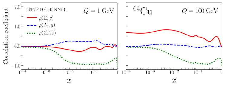
In Sect. 3 we discuss the parameterization of these three nPDFs using neural networks. In Fig. 2.2 we show the results for the correlation coefficient between the nPDFs that are parameterized in the nNNPDF1.0 fit (presented in Sect. 5), specifically the NNLO set for copper () nuclei. The nPDF correlations are computed at both GeV and GeV, the former of which contains experimental data in the region (illustrated in Fig. 2.1). In the data region, there is a strong anticorrelation between and , consistent with Eq. (2.26) which implies that only their weighted sum can be constrained. As a result, we will show in the following sections only results of the combination which can be meaningfully determined given our input experimental data. From Fig. 2.2, one can also observe the strong correlation between and for and GeV, arising from the fact that these two PDFs are coupled via the DGLAP evolution equations as opposed to and where the correlation is very weak.
3 Fitting methodology
In this section we describe the fitting methodology that has been adopted in the nNNPDF1.0 determination of nuclear parton distributions. While much of this methodology follows from previous NNPDF analyses, a number of significant improvements have been implemented in this work. Here we discuss these developments, together with relevant aspects of the NNPDF framework that need to be modified or improved in order to deal with the determination of the nuclear PDFs, such as the parameterization of the dependence or imposing the proton boundary condition.
Following the NNPDF methodology, the uncertainties associated with the nPDFs are estimated using the Monte Carlo replica method, where a large number of replicas of the experimental measurements are generated in a way that they represent a sampling of the probability distribution in the space of data. An independent fit is then performed for each of these replicas, and the resulting ensemble of nPDF samples correspond to a representation of the probability distribution in the space of nPDFs for which any statistical estimator such as central values, variances, correlations, and higher moments can be computed [4].
In order to illustrate the novel ingredients of the present study as compared to the standard NNPDF framework, we display in Fig. 3.1 a schematic representation of the tool-chain adopted to construct the nNNPDF1.0 sets. The items in blue correspond to components of the fitting methodology inherited from the NNPDF code, those in green represent new code modules developed specifically for this project, and those in yellow indicate external tools. As highlighted in Fig. 3.1, the main development is the application of TensorFlow [54], an external machine learning library that allows us access to an extensive number of tools for the efficient determination of the best-fit weights and thresholds of the neural network. The ingredients of Fig. 3.1 will be discussed in more detail in the following and subsequent sections.
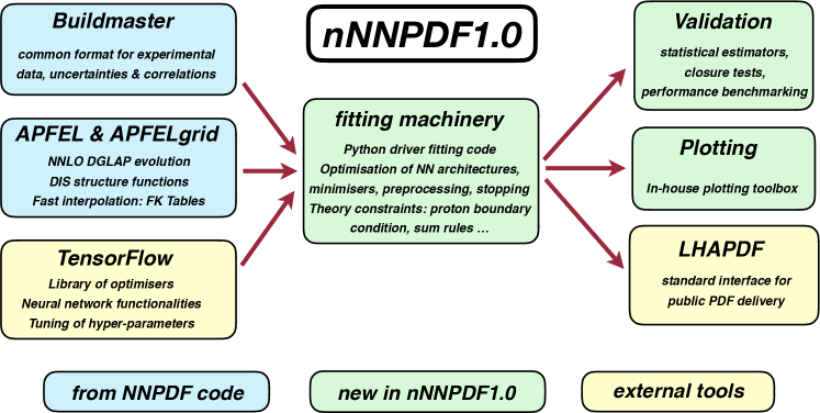
The outline of this section is the following. We start first with a discussion of our strategy for the parameterization of the nPDFs in terms of artificial neural networks. Then we present the algorithm used for the minimization of the cost function, defined to be the , which is based on stochastic gradient descent. We also briefly comment on the performance improvement obtained in this work as compared to previous NNPDF fits.
3.1 Nuclear PDF parameterization
As mentioned in Sect. 2, the non-perturbative distributions that enter the collinear factorization framework in lepton-nucleus scattering are the PDFs of a nucleon within an isoscalar nucleus with atomic mass number , . While the dependence of the nPDFs on the scale is determined by the perturbative DGLAP evolution equations, the dependence on both Bjorken- and the atomic mass number is non-perturbative and needs to be extracted from experimental data through a global analysis.111See [87] for an overview of recent efforts in the first-principle calculations of PDFs by means of lattice QCD. Taking into account the flavor decomposition presented in Sect. 2.4, we are required to parameterize the and dependence of the quark singlet , the quark octet , and the gluon , as indicated by Eq. (2.25) at LO and by Eq. (2.27) for NLO and beyond.
The three distributions listed above are parameterized at the input scale by the output of a neural network NNf multiplied by an -dependent polynomial functional form. In previous NNPDF analyses, a different multi-layer feed-forward neural network was used for each of the parameterized PDFs so that in this case, three independent neural networks would be required:
| (3.1) | |||||
However, in this work we use instead a single artificial neural network consisting of an input layer, one hidden layer, and an output layer. In Fig. 3.2 we display a schematic representation of the architecture of the feed-forward neural network used in the present analysis. The input layer contains three neurons which take as input the values of the momentum fraction , , and atomic mass number , respectively. The subsequent hidden layer contains 25 neurons, which feed into the final output layer of three neurons, corresponding to the three fitted distributions and . A sigmoid activation function is used for the neuron activation in the first two layers, while a linear activation is used for the output layer. This latter choice ensures that the network output will not be bounded and can take any value required to reproduce experimental data. The output from the final layer of neurons is then used to construct the full parameterization:
| (3.2) | |||||
where represent the values of the -th neuron’s activation state in the third and final layer of the neural network.
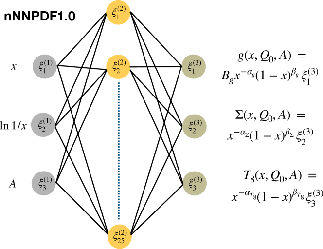
Overall, there are a total of free parameters (weights and thresholds) in the neural network represented in Fig. 3.2. These are supplemented by the normalization coefficient for the gluon nPDF and by the six preprocessing exponents and . The latter are fitted simultaneously with the network parameters, while the former is fixed by the momentum sum rule, described in more detail below. Lastly, the input scale is set to 1 GeV to maintain consistency with the settings of the baseline proton fit, chosen to be the NNPDF3.1 set with perturbative charm.
Sum rules.
Since the nucleon energy must be distributed among its constituents in a way that ensures energy conservation, the PDFs are required to obey the momentum sum rule given by
| (3.3) |
Note that this expression needs only to be implemented at the input scale , since the properties of DGLAP evolution guarantees that it will also be satisfied for any . In this analysis, Eq. (3.3) is applied by setting the overall normalization of the gluon nPDF to
| (3.4) |
where the denominator of Eq. (3.4) is computed using Eq. (3.2) and setting . Since the momentum sum rule requirement must be satisfied for any value of , the normalization factor for the gluon distribution needs to be computed separately for each value of given by the experimental data (see Table 2.1).
In addition to the momentum sum rule, nPDFs must satisfy other sum rules such as those for the valence distributions,
| (3.5) |
as well as
| (3.6) |
given the quark flavor quantum numbers of isoscalar nucleons. These valence sum rules involve quark combinations which are not relevant for the description of neutral-current DIS structure functions, and therefore do not need to be used in the present analysis. However, they will become necessary in future updates of the nNNPDF fits in which, for instance, charged-current DIS measurements are also included.
Preprocessing.
The polynomial preprocessing functions in Eq. (3.2) have long been known to approximate well the general asymptotic behavior of the PDFs at small and large [88]. Therefore, they help to increase the efficiency of parameter optimization since the neural networks have to learn smoother functions. Note that the preprocessing exponents and are independent of , implying that the entire dependence of the input nPDFs will arise from the output of the neural networks.
In previous NNPDF analyses, the preprocessing exponents and were fixed to a randomly chosen value from a range that was determined iteratively. Here instead we will fit their values for each Monte Carlo replica, so that they are treated simultaneously with the weights and thresholds of the neural network. The main advantage of this approach is that one does not need to iterate the fit to find the optimal range for the exponents, since now their best-fit values are automatically determined for each replica.
Based on basic physical requirements, as well as on empirical studies, we impose some additional constraints on the range of allowed values that the exponents and can take. More specifically, we restrict the parameter values to
| (3.7) |
Concerning the large- exponent , the lower limit in Eq. (3.7) guarantees that the nPDFs vanish in the elastic limit ; the upper limit follows from the observation that it is unlikely for the nPDFs to be more strongly suppressed at large . [88]. With respect to the small- exponent , the upper limit follows from the nPDF integrability condition, given that for the momentum integral Eq. (3.3) becomes divergent.
In addition to the conditions encoded in Eq. (3.7), we also set , namely we assume that the two quark distributions and share a similar large- asymptotic behavior. The reason for this choice is two-fold. First, we know that these two distributions are highly (anti-) correlated for neutral-current nuclear DIS observables (see Eq. (2.26)). Secondly, the large- behavior of these distributions is expected to be approximately the same, given that the strange distribution is known to be suppressed at large compared to the corresponding and distributions. In any case, it is important to emphasize that the neural network has the ability to compensate for any deviations in the shape of the preprocessing function, and therefore can in principle distinguish any differences between and in the large- region.
To illustrate the results of fitting the small and large- preprocessing exponents, we display in Fig. 3.3 the probability distributions associated with the and exponents computed using the replicas of the nNNPDF1.0 NLO set, to be discussed in Sect. 5. Here the mean value of each exponent is marked by the solid red line, and the transparent red band describes the 1- deviation. Note that these exponents are restricted to vary only in the interval given by Eq. (3.7). Interestingly, the resulting distributions for each of the and exponents turn out to be quite different, for instance is Gaussian-like while is asymmetric.
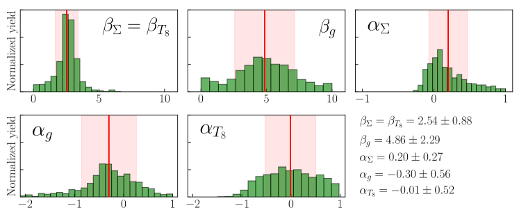
The limit of the nPDFs.
An important physical requirement that must be satisfied by the nPDFs is that they should reproduce the dependence of the PDFs corresponding to isoscalar free nucleons when evaluated at . Therefore, the following boundary conditions needs to be satisfied for all values of and :
| (3.8) |
where and indicate the parton distributions of the free proton and neutron, respectively, and are related by isospin symmetry (which is assumed to be exact). As opposed to other approaches adopted in the literature, we do not implement Eq. (3.8) at the nPDF parameterization level, but rather we impose it as a restriction in the allowed parameter space at the level of minimization, as will be discussed below. Our strategy has the crucial advantage that it assures that both central values and uncertainties of the free-nucleon PDFs will be reproduced by the nNNPDF1.0 nuclear set in the limit.
3.2 Minimization strategy
Having described the strategy for the nPDF parameterization in terms of neural networks, we turn now to discuss how the best-fit values of these parameters, namely the weights and thresholds of the neural network and the preprocessing exponents and , are determined. We also explain how we impose the boundary condition, Eq. (3.8).
In this analysis, the best-fit parameters are determined from the minimization of a function defined as
Here, and stand for the experimental data and the corresponding theoretical predictions for the nuclear ratios, respectively, the latter of which depend on the nPDF fit parameters. The covariance matrix has been defined in Eq. (2.9), and stands for the total number of data points included in the fit. Therefore, the first term above is the same as in previous NNPDF fits. Note that the first row in Eq. (3.2) could also be expressed in terms of shifts to the data or theory allowed by the correlated systematic errors [4].
Reproducing the proton PDF baseline.
The second term in Eq. (3.2) is a new feature in nNNPDF1.0. It corresponds to a quadratic penalty that forces the fit to satisfy the boundary condition in Eq. (3.8), namely that the fitted nPDFs for reproduce the PDFs of an isoscalar free nucleon constructed as the average of the proton and neutron PDFs. In order to impose this constraint in a fully consistent way, it is necessary for the proton PDF baseline to have been determined using theoretical settings and a fitting methodology that best match those of the current nPDF analysis. This requirement is satisfied by the NNPDF3.1 global analysis [71], a state-of-the-art determination of the proton PDFs based on a wide range of hard-scattering processes together with higher-order QCD calculations. Crucially, NNPDF3.1 shares most of the methodological choices of nNNPDF1.0 such as the use of neural networks for the PDF parameterization and of the Monte Carlo replica method for error propagation and estimation.
As can be seen from Eq. (3.2), this constraint is only imposed at the initial scale . This is all that is required, since the properties of DGLAP evolution will result in distributions at that automatically satisfy the constraint. The boundary condition is then constructed with a grid of values of , where 10 points are distributed logarithmically from to and 50 points are linearly distributed from to .
Note that in the low- region the coverage of this constraint is wider than that of the available nuclear data (see Fig. 2.1). Since proton PDF uncertainties, as a result of including HERA structure function data, are more reduced at small than in the corresponding nuclear case, the constraint in Eq. (3.2) introduces highly non-trivial information regarding the shape of the nPDFs within and beyond the experimental data region. Moreover, we have also verified that the constraint can also be applied down to much smaller values of , such as , by taking as a proton baseline one of the NNPDF3.0 sets which include LHCb charm production data [89, 90, 91], as will be demonstrated in Sect. 5.3.
It is important to emphasize that the boundary condition, Eq. (3.8), must be satisfied both for the PDF central values and for the corresponding uncertainties. Since proton PDFs are known to much higher precision than nPDFs, imposing this condition introduces a significant amount of new information that is ignored in most other nPDF analyses. In order to ensure that PDF uncertainties are also reproduced in Eq. (3.8), for each nNNPDF1.0 fit we randomly choose a replica from the NNPDF3.1 proton global fit in Eq. (3.2). Since we are performing a large number of fits to estimate the uncertainties in nNNPDF1.0, the act of randomly choosing a different proton PDF baseline each time guarantees that the necessary information contained in NNPDF3.1 will propagate into the nPDFs. Finally, we fix the hyper-parameter to , which is found to be the optimal setting together with the choice of architecture to yield distributions that best describe the central values and uncertainties of NNPDF3.1.
Optimization procedure.
Having defined our function in Eq. (3.2), we now move to present our procedure to determine the best-fit values of the parameters associated with each Monte Carlo replica. This procedure begins by sampling the initial values of the fit parameters. Concerning the preprocessing exponents and , they are sampled from a uniform prior in the range and for all fitted distributions. Note that these initial ranges are contained within the ranges from Eq. (3.7) in which the exponents are allowed to vary. Since the neural network can accommodate changes in the PDF shapes from the preprocessing exponents, we find the choice of the prior range from which and are initially sampled does not affect the resulting distributions. In the end, the distributions of and do not exhibit flat behavior, as is shown in Fig. (3.3).
Concerning the initial sampling of the neural network parameters, we use Xavier initialization [92], which samples from a normal distribution with a mean of zero and standard deviation that is dependent on the specific architecture of the network. Furthermore, the initial values of the neuron activation are dropped and re-chosen if they are outside two standard deviations. Since a sigmoid activation function is used for the first and second layers, this truncation of the sampling distribution ensures the neuron input to be around the origin where the derivative is largest, allowing for more efficient network training.
As highlighted by Fig. 3.1, the most significant difference between the fitting methodology used in nNNPDF1.0 as compared to previous NNPDF studies is the choice of the optimization algorithm for the minimization. In the most recent unpolarized [71] and polarized [93] proton PDF analysis based on the NNPDF methodology, an in-house Genetic Algorithm (GA) was employed for the minimization, while for the NNFF fits of hadron fragmentation functions [94] the related Covariance Matrix Adaptation - Evolutionary Strategy (CMA-ES) algorithm was used (see also [95]). In both cases, the optimizers require as input only the local values of the function for different points in the parameter space, but never use the valuable information contained in its gradients.
In the nNNPDF1.0 analysis, we utilize for the first time gradient descent with backpropagation, the most widely used training technique for neural networks (see also [43]). The main requirement to perform gradient descent is to be able to efficiently compute the gradients of the cost function Eq. (3.2) with respect to the fit parameters. Such gradients can in principle be computed analytically, by exploiting the fact that the relation between the structure functions and the input nPDFs at can be compactly expressed in terms of a matrix multiplication within the APFELgrid formalism as indicated by Eq. (2.15). One drawback of such approach is that the calculation of the gradients needs to be repeated whenever the structure of the is modified. For instance, different analytical expressions for the gradients are required if uncertainties are treated as uncorrelated and added in quadrature as opposed to the case in which systematic correlations are taken into account.
Rather than following this path, in nNNPDF1.0 we have implemented backpropagation neural network training using reverse-mode automatic differentiation in TensorFlow, a highly efficient and accurate method to automatically compute the gradients of any user-defined cost function. As a result, the use of automatic differentiation makes it significantly easier to explore optimal settings in the model and extend the analysis to include other types of observables in a global analysis.
One of the drawbacks of the gradient descent approach, which is partially avoided by using GA-types of optimizers, is the risk of ending up trapped in local minima. To ensure that such situations are avoided as much as possible, in nNNPDF1.0 we use the Adaptive Moment Estimation (ADAM) algorithm [96] to perform stochastic gradient descent (SGD). The basic idea here is to perform the training on randomly chosen subsets of the input experimental data, which leads to more frequent parameter updates. Moreover, the ADAM algorithm significantly improves SGD by adjusting the learning rate of the parameters using averaged gradient information from previous iterations. As a result, local minima are more easily bypassed in the training procedure, which not only increases the likelihood of ending in a global minima but also significantly reduces the training time.
In this analysis, most of the ADAM hyper-parameters are set to be the default values given by the algorithm, which have been tested on various machine learning problems. This includes the initial learning rate of the parameters, , the exponential decay rate of the averaged squared gradients from past iterations, , and a smoothing parameter . However, we increase the exponential decay rate of the mean of previous gradients, , which can be interpreted more simply as the descent momentum. This choice was observed to improve the performance of the minimization overall, as it exhibited quicker exits from local minima and increased the rate of descent.
Given that our neural-network-based parameterization of the nPDFs, Eq. (3.2), can be shown to be highly redundant for the current input dataset (see also Sect. 5.3), we run the risk of fitting the statistical fluctuations in the data rather than the underlying physical law. To prevent such overfitting, we have implemented the look-back cross-validation stopping criterion presented for the first time in NNPDF fits in Ref. [7]. The basic idea of this algorithm is to separate the input dataset into disjoint training and validation datasets (randomly chosen replica by replica), minimize the training set function, , and stop the training when the validation , , reveals a global minimum. In this analysis, the data is partitioned 50%/50% to construct each of the two sets, except for experiments with 5 points or less which are always included in the training set.
The final fits are chosen to satisfy simultaneously,
| (3.10) | |||
where and are the number of data points in the training and validation sets, respectively, and corresponds to the second term in Eq. 3.2. Upon reaching the above conditions during minimization, checkpoints are saved for every 100 iterations. A fit is then terminated when a smaller value for the validation is not obtained after iterations, or when the fit has proceeded iterations (early stopping). The former is set to allow sufficient time to escape local minima, and the latter is set due to the SGD algorithm, which can fluctuate the parameters around the minimum indefinitely. In either case the fit is considered successful, and the parameters that minimize are selected as the best-fit parameters (look-back).
While automatic differentiation with TensorFlow is the baseline approach used to construct the nNNPDF1.0 sets, during this work we have also developed an alternative C++ fitting framework that uses the ceres-solver optimizer interfaced with analytical calculations of the gradients of the function. The comparison between the analytical and automated differentiation strategies to compute the gradients and to carry out the minimization of Eq. (3.2) will be presented elsewhere [97], together with a comparison of the performance and benchmarking between these two approaches.
Performance benchmarking.
While a detailed and systematic comparison between the performances of the TensorFlow-based stochastic gradient descent optimization used in nNNPDF1.0 and that of the GA and CMA-ES minimizers used in previous NNPDF analyses is beyond the scope of this work, here we provide a qualitative estimate for improvement in performance that has been achieved as a result of using the former strategy.
In order to assess the performance of these two strategies, we have conducted two Level-0 closure tests (see Sect. 4 for more details) on the same computing machine. For the first test, a variant of the nNNPDF1.0 fit was run without the constraint and with the preprocessing exponents fixed to randomly selected values within a specific range. For the second, a variant of the NNPDF3.1 DIS-only fit was run with kinematic cuts adjusted so that they match the value of used in the first fit. Moreover, the preprocessing exponents are fixed in the same manner. To further ensure similar conditions as much as possible with the nNNPDF1.0-like fits, the fitting basis of NNPDF3.1 has been reduced to that composed by only and , while the architecture of the networks has been modified so that the number of fitted free parameters is the same in both cases. While these common settings are suitable for a qualitative comparison between the two optimizers, we want to emphasize that the results should not be taken too literally, as other aspects of the two fits are slightly different.
In Fig. 3.4 we show the results of this benchmark comparison for the performance of the TensorFlow-based stochastic gradient descent optimization with that of the Genetic Algorithm (labelled NGA) used in NNPDF3.1. Within a Level-0 closure test, we monitor the average time it takes each optimizer to reach a given target. We then plot the ratio of the average SGD time with the corresponding GA result. For a conservative target, , the NGA appears to perform better than SGD. This is a well-known property of evolutionary algorithms: they manage to rather quickly bring the parameter space to the vicinity of a minimum of the cost function.
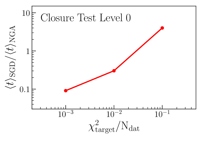
The real power of SGD becomes apparent once a more stringent target is set. As will be described in more detail in the following section, the figure of merit in Level 0 closure tests can be arbitrarily reduced until asymptotically the limit is reached. We find that in this case, the average time for SGD can be significantly smaller than the corresponding NGA time. For , the speed improvement is around an order of magnitude, and from the trend it is apparent that this improvement would continue for new targets. The benchmark comparison of Fig. 3.4 highlights how, with the use of SGD, it becomes possible to explore the vicinity of minima in a more efficient way than NGA, thus bringing in a considerable speed improvement that can reach a factor of 10 or more.
4 Closure Tests
Since a significant amount of the fitting methodology used to construct nNNPDF1.0 has been implemented for the first time in this analysis, it is important to test its performance and demonstrate its reliability using closure tests. The general idea of closure tests is to carry out fits based on pseudo-data generated with a known underlying theory. In this case, an existing nPDF set is used and the fit results are compared with this “true” result using a variety of statistical estimators. In addition, the exercise is performed within a clean environment which is not affected by other possible effects that often complicate global fits, such as limitations of the theory calculations or the presence of internal or external data inconsistencies.
In this section, we briefly outline the different types closure tests that we have performed to validate the nNNPDF1.0 fitting methodology. The nomenclature and settings for the different levels of closure tests follows Ref. [7] (see also [98] for a related discussion in the context of SMEFT analyses).
For all of the closure tests presented in this section, the fitting methodology is identical to that used for the actual nNNPDF1.0 analysis and was described in the previous section. The differences between the different closure fits are then related to the generation of the pseudo-data. The underlying distributions have been chosen to be those from the nCTEQ15 analysis, from which the pseudo-data is constructing by evaluating predictions for the nuclear structure functions using the theoretical formalism in Sect. 2. Furthermore, the deuteron structure functions are constructed from the NNPDF3.1 proton PDF set so that only the numerator is fitted in the ratios. The nPDFs to be determined by the fit are then parameterized at the input scale GeV (rather than 1 GeV) to maintain the consistency with the settings of nCTEQ15. Lastly, we do not impose our boundary condition at , since our aim is not to achieve the smallest possible uncertainties but instead to show that we are able to reproduce the input distributions from nCTEQ15.
4.1 Level 0
We start by presenting the results of the simplest type of closure test, Level 0 (L0), and then discuss how these are modified for the more sophisticated Level 1 (L1) and Level 2 (L2) fits. At Level 0, the pseudo-data is generated from the nCTEQ distributions without any additional statistical fluctuations, and the uncertainties are taken to be the same as the experimental data. The is then defined to be the same as in the fits to real data, taking into account all sources of experimental uncertainties in the covariance matrix Eq. (2.9). Moreover, there are no Monte Carlo replicas, and closure tests are carried out times for different random values of the initial fit parameters. The variance of the fits then defines the PDF uncertainties at this level. By defining the closure test Level 0 in this way, there is guaranteed to exist at least one possible solution for the fit parameters which result in , where the fitted nPDFs coincide with nCTEQ15. Therefore a key advantage of this test is its ability to assess the flexibility of the chosen input functional form and determine whether the shapes of the underlying distributions are able to be reproduced.
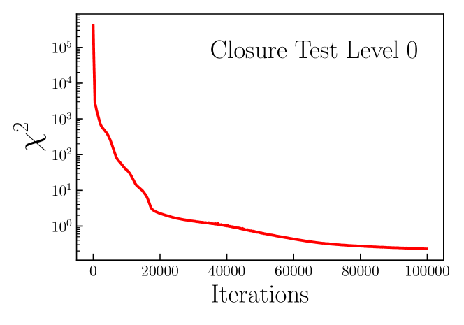
Due to the absence of statistical fluctuations in the pseudo-data, overlearning is not possible. Consequently, the fits are performed without cross-validation and early stopping, and the maximum number of iterations a given fit can progress is a free parameter that can be chosen to be arbitrarily large. Although the value of the total with respect to the number of iterations may flatten as the maximum number of iterations is increased and one is close to the absolute minimum, the should continue to vanish asymptotically provided the optimizer is adequately efficient.
To demonstrate that these expectations are indeed satisfied in our case, we display in Fig. 4.1 the value of the total as a function of the number of iterations proceeded in the minimization process for a specific choice of the initial conditions of the fit parameters. We find the results for other initial conditions are qualitatively similar. For this case, the decreases monotonically with the number of iterations without ever saturating. Note also how the rate of decrease of the is high for low number of iterations, but becomes slower as the number of iterations is increased. This behavior is expected since it is more difficult to find directions in the parameter space close to the minimum that further reduce the cost function. The final results are chosen to satisfy after a maximum number of iterations of .
In Fig. 4.2, we show the resulting nPDFs from a Level 0 closure test. Here the quark combination and the gluon are plotted as a function of at the initial evolution scale GeV for and . We also display the 1- uncertainties computed over the replicas, while for the input nCTEQ distributions only the central values are shown. Since the aim of closure tests is not to reproduce the uncertainties of the prior distributions but rather the central values used to generate the pseudo-data, the nCTEQ uncertainties are not relevant here and therefore we do not show them in any of the results presented in this section.
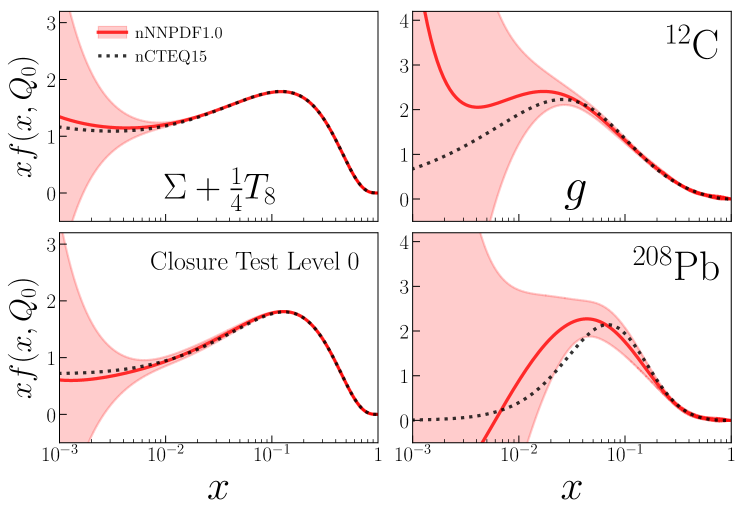
As we can see from the comparison in Fig. 4.2, there is a very good agreement between the central values of both the quark combination and the gluon with the nCTEQ15 prior in the data region. This is especially marked for the quark distribution, given that it is directly constrained by the structure function measurements. Concerning the gluon nPDF, which is only constrained indirectly from data, the agreement is somewhat better for than for for which there are very limited experimental constraints. This behavior can be understood by the fact that the gluon for is much less constrained by the available data than for , and thus even in a perfect L0 closure test, with , one can expect small deviations with respect to the underlying physical distributions. Nevertheless, our results agree overall with the nCTEQ15 central values and the L0 closure test is considered successful.
4.2 Level 1
We continue now to discuss the results of the Level 1 closure tests. In this case, the pseudo-data is generated by adding one layer of statistical fluctuations to the nCTEQ15 predictions. These fluctuations are dictated by the corresponding experimental statistical and systematic uncertainties, and are the same that enter in the covariance matrix Eq. (2.9). In other words, we take the L0 pseudo-data and add random noise by Gaussian smearing each point about the corresponding experimental uncertainties. As in the L0 closure tests, the same pseudo-data set is used to perform an number of fits, each with a different initialization of the fit parameters, and the resulting variance defines the nPDF uncertainties. Due to the Gaussian smearing, however, over-learning is now possible at Level 1 and therefore cross-validation with early stopping is required. As a result, the optimal fit parameters are expected to give instead .
In Fig. 4.3 we show a similar comparison as that of Fig. 4.2 but now for the L1 closure tests. While the level of agreement with the nCTEQ15 prior is similar as in the case of L0 fits, the PDF uncertainties have now increased, especially for the gluon nPDF. This increase at L1 reflects the range of possible solutions for the initial nPDFs at that lead to a similar value of . Therefore, the L1 test not only allows us to verify that the input distributions are reproduced, but also that the added statistical fluctuations at the level of the generated pseudo-data are reflected in the resulting uncertainties.
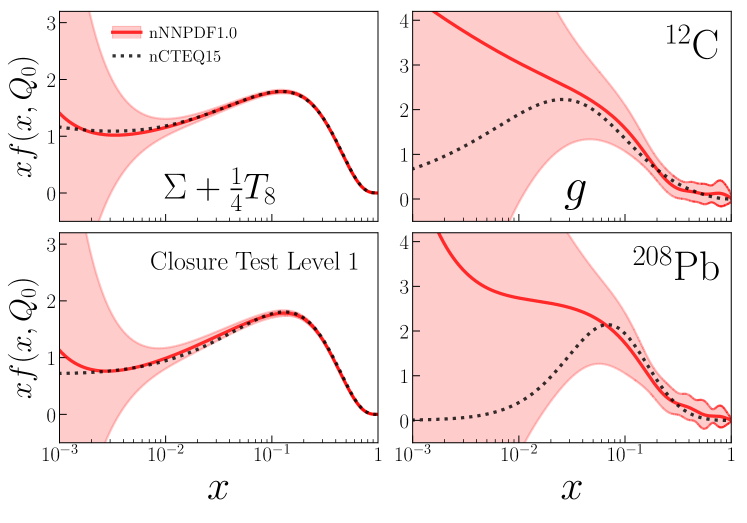
In Table 4.1 we list the averaged values for in the L1 closure test compared with the corresponding values obtained with the prior theory. As expected, we find the values at L1 being close to those of the prior both at the level of the total dataset as well as that of individual experiments. The agreement is particularly good for datasets with a large number of points that carry more weight in the fit. In summary, the comparison in Fig. 4.3 combined with that in Table 4.1 demonstrate the closure tests are also successful at L1.
| Experiment | (L1CT) | (prior) | ||
|---|---|---|---|---|
| SLAC E-139 | 4He/2D | 3 | 0.94 | 2.61 |
| NMC 95, re. | 4He/2D | 13 | 1.83 | 1.17 |
| NMC 95 | 6Li/2D | 12 | 0.97 | 0.87 |
| SLAC E-139 | 9Be/2D | 3 | 0.66 | 0.09 |
| NMC 96 | 9Be/12C | 14 | 1.04 | 0.99 |
| EMC 88, EMC 90 | 12C/2D | 12 | 0.45 | 0.47 |
| SLAC E-139 | 12C/2D | 2 | 0.52 | 0.80 |
| NMC 95, NMC 95, re. | 12C/2D | 26 | 1.79 | 1.79 |
| FNAL E665 | 12C/2D | 3 | 1.07 | 0.84 |
| NMC 95, re. | 12C/6Li | 9 | 0.71 | 0.54 |
| BCDMS 85 | 14N/2D | 9 | 0.81 | 0.77 |
| SLAC E-139 | 27Al/2D | 3 | 2.42 | 3.14 |
| NMC 96 | 27Al/12C | 14 | 1.18 | 1.26 |
| SLAC E-139 | 40Ca/2D | 2 | 1.24 | 1.36 |
| NMC 95, re. | 40Ca/2D | 12 | 2.07 | 1.87 |
| EMC 90 | 40Ca/2D | 3 | 3.18 | 3.23 |
| FNAL E665 | 40Ca/2D | 3 | 0.23 | 0.23 |
| NMC 95, re. | 40Ca/6Li | 9 | 0.46 | 0.41 |
| NMC 96 | 40Ca/12C | 23 | 1.22 | 1.20 |
| EMC 87 | 56Fe/2D | 58 | 0.60 | 0.59 |
| SLAC E-139 | 56Fe/2D | 8 | 0.66 | 0.57 |
| NMC 96 | 56Fe/12C | 14 | 1.35 | 1.05 |
| BCDMS 85, BCDMS 87 | 56Fe/2D | 16 | 0.82 | 0.70 |
| EMC 88, EMC 93 | 64Cu/2D | 27 | 1.32 | 1.38 |
| SLAC E-139 | 108Ag/2D | 2 | 0.33 | 0.28 |
| EMC 88 | 119Sn/2D | 8 | 0.12 | 0.13 |
| NMC 96, dependence | 119Sn/12C | 119 | 0.95 | 0.98 |
| FNAL E665 | 131Xe/2D | 4 | 0.99 | 0.84 |
| SLAC E-139 | 197Au/2D | 3 | 0.21 | 0.31 |
| FNAL E665 | 208Pb/2D | 3 | 1.29 | 1.31 |
| NMC 96 | 208Pb/12C | 14 | 0.98 | 0.90 |
| Total | 451 | 1.03 | 1.00 |
4.3 Level 2
In L2 closure tests, the pseudo-data generated in the L1 case is now used to produce a large number of Monte Carlo replicas. A nuclear PDF fit is then performed for each replica, and look-back cross-validation is again activated to prevent over-fitting. The procedure at L2 therefore matches the one applied to real data to determine the nNNPDF1.0 set of nPDFs, so that the statistical and systematic uncertainties provided by the experimental measurements are propagated into the resulting nPDF uncertainties. By comparing the PDF uncertainties at L2 with those at L1 and L0, one can disentangle the various contributions to the total nPDF error, as we discuss in more detail below.
Given the extra layer of statistical fluctuations introduced by the Monte Carlo replica generation, at L2 the figure of merit for each replica is , where indicates the number of data points in the training (validation) set. In Fig. 4.4, we show a similar plot as in Fig. 4.1 but now for a representative replica from the Level 2 closure test. Here the values from the training and validation samples are plotted separately, and the vertical dashed line indicates the stopping point, defined to be the absolute minimum of , at which the optimal parameters are taken. Since we have and , we find as expected.
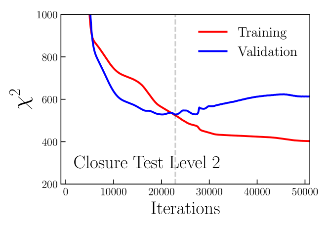
Fig. 4.4 clearly illustrates the importance of cross-validation stopping. For a low number of iterations, both and are similar in size and decrease monotonically: this corresponds to the learning phase. However, beyond a certain point the keeps decreasing while the instead begins to increase, indicating that the statistical fluctuations rather than the underlying distributions are being fitted. As a result of using cross-validation, we are able to avoid over-fitting and ensure that for each replica the minimization is stopped at the optimal number of iterations.
In Fig. 4.5, a similar comparison as that of Fig. 4.2 is shown, where now the nPDFs at the initial parameterization scale GeV obtained from the L0, L1, and L2 closure tests are displayed together. Here the nCTEQ15 prior agrees well with the central values of all the closure tests. Moreover, it is important to note that the nPDF uncertainties are smallest at Level 0 and then increase subsequently with each level. The comparison of the results for the different levels of closure tests can be interpreted following the discussions of [7].
First of all, at L0 the PDF uncertainty within the data region should go to zero as the number of iterations is increased due to the fact that , as illustrated in Fig. 4.1. While the PDF uncertainties will generally decrease with the number of iterations, this may not necessarily be true between data points (interpolation) and outside the data region (extrapolation). The latter is known as the extrapolation uncertainty, and is present even for a perfect fit for which the vanishes. In our fits, the extrapolation region can be assessed from Fig. 2.1, where and are not directly constrained from any measurement in nNNPDF1.0.
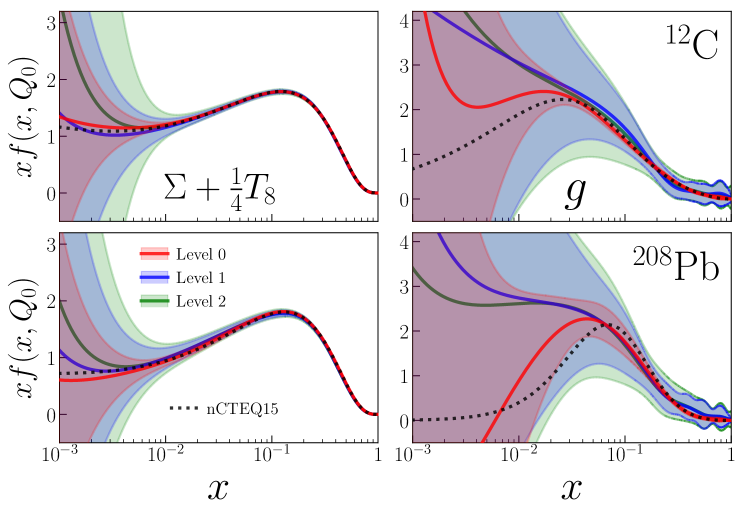
In a L1 fit, the central values of the data have been fluctuated around the theoretical predictions from nCTEQ15. This means that now there can exist many functional forms for the nPDFs at that have equally good values. The difference between the PDF uncertainties at L0 and L1 is thus known as the functional uncertainty. Finally, at L2 one is adding on top of the L1 pseudo-data the Monte Carlo replica generation reflecting the statistical and systematic errors provided by the experimental measurements. This implies that the difference between L1 and L2 uncertainties can be genuinely attributed to the experimental data errors, and is therefore known as the data uncertainty. Comparing the resulting nPDFs for various levels of closure tests, as in Fig. 4.5, allows us to discriminate the relative importance of the extrapolation, function, and data components to the total nNNPDF1.0 uncertainty band.
From the comparison of Fig. 4.5, we see that the extrapolation uncertainty is very small for the quarks except for where indeed experimental data stops. The same applies for the gluon for , while for the extrapolation (L0) uncertainty becomes large already at . Interestingly, there is a big increase in uncertainties when going from L0 to L1 for the gluon distribution: this highlights how functional uncertainties represent by far the dominant component in the PDF uncertainty for most of the relevant kinematic range. Lastly, differences between L1 and L2 are quite small, and therefore the experimental data errors propagated by the MC replicas contributes little to the overall uncertainties. Nevertheless, it is an important component and must be included for a robust estimation of the nPDF uncertainties.
5 Results
In this section we present the main results of our analysis, namely the nNNPDF1.0 sets of nuclear parton distributions. We first assess the quality of our fit by comparing the resulting structure function ratios with experimental data. This is followed by a discussion of the main features of the nNNPDF1.0 sets, as well as a comparison with the recent EPPS16 and nCTEQ15 nPDF analyses. We also assess the stability of our results with respect to the perturbative order, which are generated using NLO and NNLO QCD theories. Finally, the section is concluded by presenting a few methodological validation tests, complementing the closure test studies discussed in Sect. 4. Here we show that our results are stable with respect to variations of the network architecture and quantify the impact of the boundary condition.
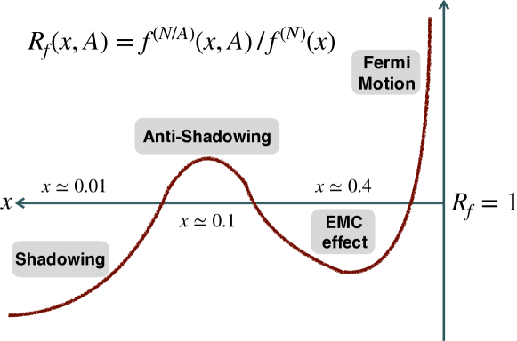
Before moving forward, it is useful to illustrate qualitatively the expected outcome for a nuclear PDF analysis. In Fig. 5.1 we show a schematic representation of different types of nuclear modifications that are assumed to arise in the nPDFs, , when presented as ratios to their free-nucleon counterparts ,
| (5.1) |
The ratio defined here corresponds to the nPDF equivalent of the structure function ratios, Eq. (2.5), where signifies the absence of nuclear modifications. Moving from small to large , a depletion known as shadowing is expected, followed by an enhancement effect known as anti-shadowing. For the region , there is expected to be a suppression related to the original EMC effect, while at larger there should be a sharp enhancement as a result of Fermi motion. In presenting the results of the nNNPDF1.0 PDF sets, the discussion will focus primarily on whether the different nuclear effects shown in Fig. 5.1 are supported by experimental data and how the various effects compare between the quark and gluon distributions.
5.1 Comparison with experimental data
To begin, we list in Table 5.1 the absolute and normalized values of the for each of the input datasets (see Table 2.1) and for the total dataset. The values are given for both the NLO and NNLO fits. In total, there are data points that survive the kinematic cuts and result in the overall value , indicating an excellent agreement between the experimental data and the theory predictions. Moreover, we find that the fit quality is quite similar between the NLO and NNLO results. The fact that we obtain an overall less than one can be attributed to the absence of correlations between experimental systematics, leading to an overestimation of the total error.
| Experiment | NLO | NNLO | ||||
|---|---|---|---|---|---|---|
| SLAC E-139 | 4He/2D | 3 | 1.49 | 0.50 | 1.50 | 0.50 |
| NMC 95, re. | 4He/2D | 13 | 12.81 | 1.0 | 12.79 | 0.98 |
| NMC 95 | 6Li/2D | 12 | 10.96 | 0.91 | 10.50 | 0.88 |
| SLAC E-139 | 9Be/2D | 3 | 2.91 | 0.97 | 2.91 | 0.97 |
| NMC 96 | 9Be/12C | 14 | 4.03 | 0.29 | 4.06 | 0.29 |
| EMC 88, EMC 90 | 12C/2D | 12 | 12.98 | 1.08 | 13.04 | 1.09 |
| SLAC E-139 | 12C/2D | 2 | 0.65 | 0.33 | 0.74 | 0.37 |
| NMC 95, NMC 95, re. | 12C/2D | 26 | 25.12 | 0.97 | 24.81 | 0.95 |
| FNAL E665 | 12C/2D | 3 | 3.13 | 1.04 | 3.13 | 1.04 |
| NMC 95, re. | 12C/6Li | 9 | 6.62 | 0.74 | 6.25 | 0.69 |
| BCDMS 85 | 14N/2D | 9 | 11.10 | 1.23 | 11.16 | 1.24 |
| SLAC E-139 | 27Al/2D | 3 | 0.52 | 0.17 | 0.65 | 0.22 |
| NMC 96 | 27Al/12C | 14 | 4.34 | 0.31 | 4.31 | 0.31 |
| SLAC E-139 | 40Ca/2D | 2 | 2.79 | 1.40 | 2.95 | 1.48 |
| NMC 95, re. | 40Ca/2D | 12 | 11.75 | 0.98 | 11.86 | 0.99 |
| EMC 90 | 40Ca/2D | 3 | 4.11 | 1.37 | 4.09 | 1.36 |
| FNAL E665 | 40Ca/2D | 3 | 5.07 | 1.69 | 4.77 | 1.59 |
| NMC 95, re. | 40Ca/6Li | 9 | 2.18 | 0.24 | 2.05 | 0.23 |
| NMC 96 | 40Ca/12C | 23 | 13.20 | 0.57 | 13.26 | 0.58 |
| EMC 87 | 56Fe/2D | 58 | 36.89 | 0.63 | 37.12 | 0.64 |
| SLAC E-139 | 56Fe/2D | 8 | 11.01 | 1.38 | 11.20 | 1.4 |
| NMC 96 | 56Fe/12C | 14 | 9.21 | 0.66 | 9.00 | 0.64 |
| BCDMS 85, BCDMS 87 | 56Fe/2D | 16 | 9.48 | 0.6 | 9.53 | 0.6 |
| EMC 88, EMC 93 | 64Cu/2D | 27 | 12.56 | 0.47 | 12.63 | 0.47 |
| SLAC E-139 | 108Ag/2D | 2 | 1.04 | 0.52 | 1.04 | 0.52 |
| EMC 88 | 119Sn/2D | 8 | 17.77 | 2.22 | 17.71 | 2.21 |
| NMC 96, dependence | 119Sn/12C | 119 | 59.24 | 0.50 | 58.28 | 0.49 |
| FNAL E665 | 131Xe/2D | 4 | 1.47 | 0.37 | 1.45 | 0.36 |
| SLAC E-139 | 197Au/2D | 3 | 2.46 | 0.82 | 2.33 | 0.78 |
| FNAL E665 | 208Pb/2D | 3 | 4.97 | 1.66 | 5.10 | 1.7 |
| NMC 96 | 208Pb/12C | 14 | 5.23 | 0.37 | 5.61 | 0.4 |
| Total | 451 | 307.1 | 0.68 | 305.82 | 0.68 | |
At the level of individual datasets, we find in most cases a good agreement between the experimental measurements and the corresponding theory calculations, with many both at NLO and at NNLO. The agreement is slightly worse for the ratios Ca/D and Pb/D from FNAL E665, as well as the Sn/D ratio from EMC, all of which have . The apparent disagreement of these datasets can be more clearly understood with the visual comparison between data and theory.
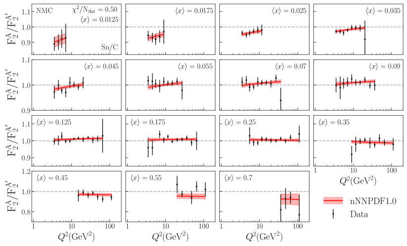
In Fig. 5.2 we display the structure function ratios measured by the EMC and NMC experiments and the corresponding theoretical predictions from the nNNPDF1.0 NLO fit. Furthermore, in Figs. 5.3 and 5.4 we show the corresponding comparisons for the -dependent structure function ratio provided by the NMC experiment, and the data provided by the BCDMS, FNAL E665, and SLAC-E139 experiments, respectively.
In the comparisons shown in Figs. 5.2–5.4, the central values of the experimental data points have been shifted by an amount determined by the multiplicative systematic uncertainties and their nuisance parameters, while uncorrelated uncertainties are added in quadrature to define the total error bar. We also indicate in each panel the value of , which include the quadratic penalty as a result of shifting the data to its corresponding value displayed in the figures. The quoted values therefore coincide with those of Eq. (3.2) without the penalty term. Lastly, the theory predictions are computed at each and bin given by the data, and its width corresponds to the 1- deviation of the observable using the nNNPDF1.0 NLO set with replicas. Note that in some panels, the theory curves (and the corresponding data points) are shifted by an arbitrary factor to improve visibility.
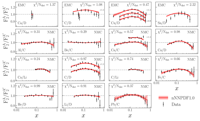
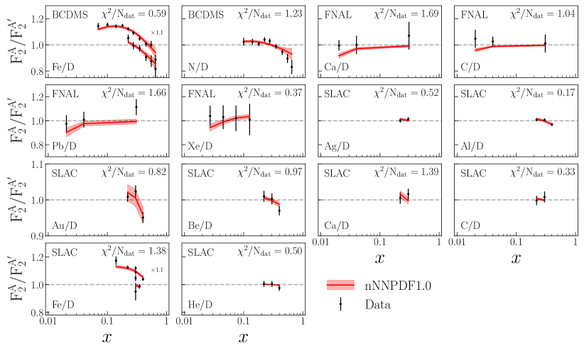
As expected by the values listed in Table 5.1, the experimental measurements agree well with the structure function ratios computed using the nNNPDF1.0 sets, apart from the three observables mentioned previously. For the FNAL data, the disagreement comes from datasets that contain a total of 3 data points with larger uncertainties than other experimental measurements, and therefore do not significantly impact the fit results.
A similar argument can be made for the Sn/D ratio from the EMC experiment, which has . Here the lack of agreement between theory and data can be traced to the low- region of the structure function ratio. Such a deviation can also be seen in the recent nCTEQ and EPPS analyses, and can be attributed to a possible tension with the dependent ratio Sn/C presented in Fig. 5.3. While the comparison here is with carbon and not deuterium, the nuclei are relatively close in mass number and therefore the effects in the ratio are expected to be similar. On the other hand, the data show a roughly difference between EMC’s Sn/D and NMC’s Sn/C at . Since the NMC data have smaller uncertainties than EMC, its influence on the fit is much stronger, driving the disagreement with EMC Sn/D at low . Overall, the agreement with NMC data is excellent, including the dependent Sn/C data presented in Fig. 5.3.
From the data versus theory comparisons, the various nuclear effects encoded in the structure function ratios can clearly be observed. At small the structure functions exhibit shadowing, namely the depletion of compared to its free-nucleon counterpart (or compared to lighter nuclei). At larger the well known EMC effect is visible, resulting in ratios below unity. Between these two regimes, one finds an enhancement of the nuclear structure functions. However, we do not observe the Fermi motion effect, which gives for large and increases rapidly in the limit. This is due simply to the kinematic cut illustrated in Fig. 2.1, which removes much of the large- data. Note that although the three nuclear regimes are visible at the structure function level, such effects may not be reflected at the level of PDF ratios, as we will highlight in the following section.
5.2 The nNNPDF1.0 sets of nuclear PDFs
With the agreement between data and theory established, we present now the results for the NLO nPDF sets. Later, we will assess the perturbative stability of the results by comparing to the corresponding NNLO fit. Unless otherwise indicated, the results presented in this section are generated with Monte Carlo replicas.
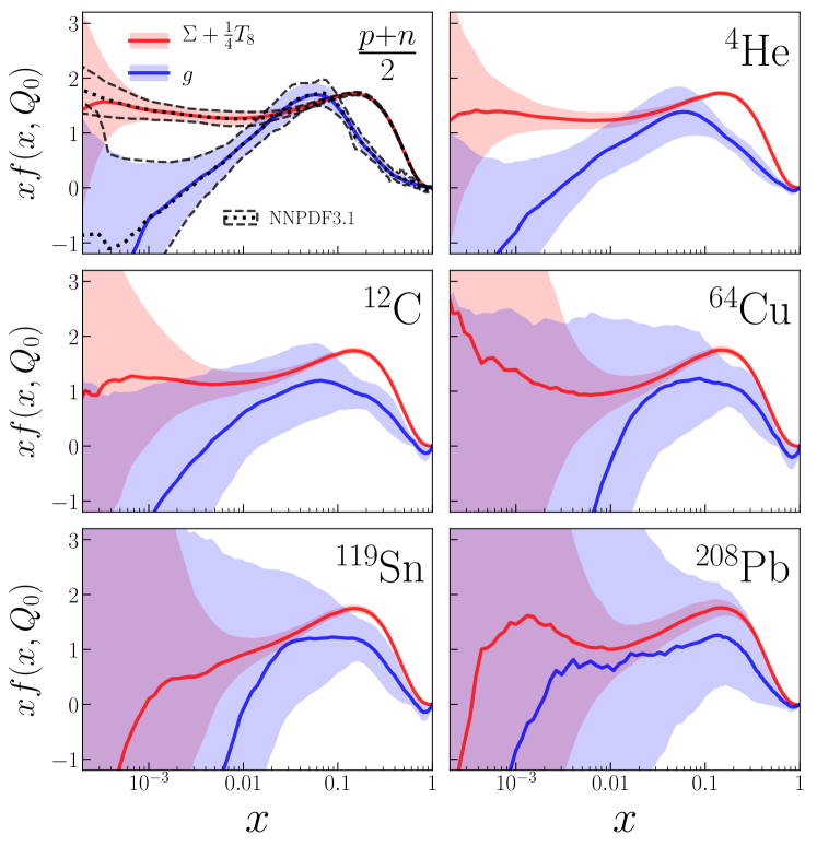
To begin, we show in Fig. 5.5 the nNNPDF1.0 NLO set as a function of at the input scale GeV for different values of . In this figure, the nPDF uncertainty bands are computed as the 90% confidence level intervals, with the central value being taken as the midpoint of the corresponding range. The confidence levels presented here follow that of previous NNPDF studies [49] and are computed in the following way. For a given , , and , we have values of a particular nPDF flavor . The replicas are then ordered such that
| (5.2) |
Finally, we remove symmetrically of the replicas with the highest and lowest values. The resulting interval defines the confidence level for the nPDF for a given value of , , and . In other words, a 90% CL interval (corresponding to a 2- interval for a Gaussian distribution) is obtained by keeping the central 90% replicas, leading to
| (5.3) |
The rationale for estimating the nPDF uncertainties as 90% CL intervals, as opposed to the standard deviation, is that it turns out that the nNNPDF1.0 probability distribution is not well described by a Gaussian, in particular when ratios between different nuclei are taken. Therefore, the variance may not be the best estimator for the level of fluctuations in the distribution. While deviations from the Gaussian approximation in the proton case are moderate, there are several reasons why the nPDFs may behave differently. First of all, there is a limited amount of experimental information, especially for the gluon. Secondly, imposing the boundary condition skews the dependence of the distribution. Lastly, even if the resulting nPDFs do follow a Gaussian distribution, in general their ratio between different values of will not. Therefore, in Fig. 5.5, and in the remaining figures of this analysis, the uncertainties will be presented as the 90% CL defined above.
We also show in Fig. 5.5 the results of the baseline free-nucleon PDF set, NNPDF3.1, compared to the nuclear parton distributions evaluated at . As can be observed, there is an excellent match between both the central values and the PDF uncertainties of nNNPDF1.0 and those of NNPDF3.1 in the region of where the boundary condition is imposed, . This agreement demonstrates that the quadratic penalty in Eq. (3.2) is sufficient to achieve its intended goals. In Sect. 5.3 we will discuss the importance of implementing such a constraint, particularly for light nuclei.
From Fig. 5.5, we can also see that the PDF uncertainties increase as we move towards larger values of , in particular for the gluon nPDF. Recall that the latter is only constrained indirectly from inclusive DIS data via DGLAP evolution effects. On the other hand, the quark combination turns out to be reasonably well constrained for , since this is the combination directly related to the nuclear structure function . For both the gluon and the quark nuclear distributions, the PDF uncertainties diverge in the small- extrapolation region, the beginning of which varies with . For example, the extrapolation region for the quarks in Sn () is found to be , while for the gluon PDF uncertainties become very large already for .
Next, we illustrate in Fig. 5.6 the nNNPDF1.0 PDFs normalized by the distributions. Here the results for He (), Cu (), and Pb () nuclei are shown for GeV2. With this comparison, we can assess whether the different nuclear effects introduced previously are visible at the nPDF level, since Eq. (3.2) is analagous to the structure function ratios displayed in Figs. 5.2–5.4.
When evaluating ratios of nPDFs between different values of , it is important to account for the correlations between the numerator and denominator. These correlations stem from the fact that nPDFs at two values of are related by the common underlying parameterization, Eq. (3.2), and therefore are not independent. This can be achieved by computing the ratio for each of the Monte Carlo replicas of the fit
| (5.4) |
and then evaluating the 90% CL interval following the procedure that leads to Eq. (5.3). Note that a rather different result from that of Eq. (5.4) would be obtained if either the correlations between different values were ignored (and thus the PDF uncertainties in numerator and denominator of Eq. (5.1) are added in quadrature) or if the uncertainties associated to the denominator were not considered. Also, as discussed above, the 90% CL interval for Eq. (5.4) will in general be quite different compared to the range defined by the 2- deviation.
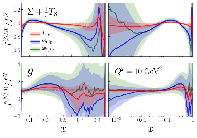
From Fig. 5.6, we can see that for the relevant quark combination in and nuclei, it possible to identify the same three types of nuclear effects that were present at the structure function level. In particular, the anti-shadowing and EMC effects are most evident, where the deviation from unity is outside the 90% CL range. Moreover, shadowing behavior appears briefly in the region , particularly for copper nuclei, before the uncertainties grow quickly in the extrapolation region. On the other hand, the nuclear effects appear to be negligible for all in helium nuclei within the present uncertainties.
The situation is much worse for the nuclear gluons, where the ratio is consistent with one within the uncertainties for all values of . This indicates that using only neutral-current DIS nuclear structure functions, there is limited information that one can extract about the nuclear modifications of the gluon PDF. Here we find no evidence for gluon shadowing, and the ratio is consistent with one for . The only glimpse of a non-trivial nuclear modification of the gluon nPDF is found for Cu (), where between and there appears to be an enhancement reminiscent of the anti-shadowing effect.
The comparisons of Fig. 5.6 demonstrate that, without additional experimental input, we are rather far from being able to probe in detail the nuclear modifications of the quark and gluon PDFs, particularly for the latter case. We will highlight in Sect. 6 how the present situation would be dramatically improved with an Electron Ion Collider, allowing us to pin down nuclear PDFs in a wider kinematic range and with much better precision.
The scale dependence of the nuclear modifications.
In Fig. 5.7, we show a similar comparison as that of Fig. 5.6, but now for the dependence of the nuclear modifications in 64Cu. More specifically, we compare the results of nNNPDF1.0, normalized as before to the distribution, for GeV2, 10 GeV2, and 100 GeV2. We can observe in this case how nPDF uncertainties are reduced when the value of is increased. This effect is particularly dramatic for the gluon in the small- region, but is also visible for the quark distributions. This feature is a direct consequence of the structure of DGLAP evolution, where at small and large the results tend to become insensitive of the specific boundary condition at low scales as a result of double asymptotic scaling [99].
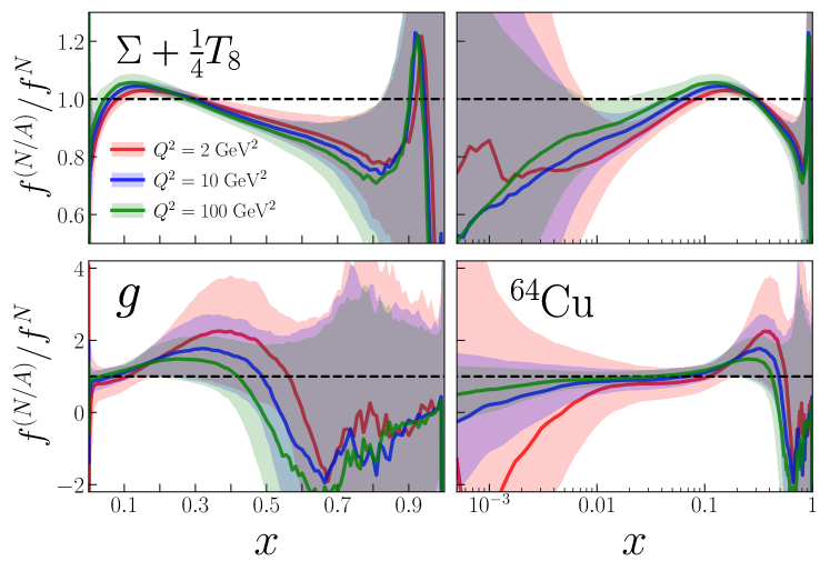
It is important to point out that, by the same token, the sensitivity to nuclear modifications is also reduced when going from low to high in the small- region. Indeed, we can see from Fig. 5.7 that the ratios move closer to one at small as is increased. However, this is not the case for medium and large , where DGLAP evolution effects are milder. Therefore, nuclear effects in this region can be accessible using probes both at low and high momentum transfers. The comparisons in Fig. 5.7 highlight that the best sensitivity for nuclear modifications present in the small- region arises from low-scale observables, while for medium and large- modifications there is also good sensitivity at high scales.
Comparison with EPPS16 and nCTEQ15.
We now turn to compare the nNNPDF1.0 nuclear PDFs with other recent analyses. Here we restrict our comparison to the EPPS16 and nCTEQ15 fits, given that they are the only recent nPDF sets available in LHAPDF. In Fig. 5.8, we display the nNNPDF1.0 NLO distributions together with EPPS16 and nCTEQ15 at GeV2 for three different nuclei: 12C, 64Cu, and 208Pb. The three nPDF sets have all been normalized to the central value of their respective proton PDF baseline to facilitate the comparison. For the nNNPDF1.0 results, the uncertainties are computed as before but without including the correlations with the distribution. Lastly, the PDF uncertainties for EPPS16 and nCTEQ15 correspond to the 90% CL ranges computed using the standard Hessian prescription.
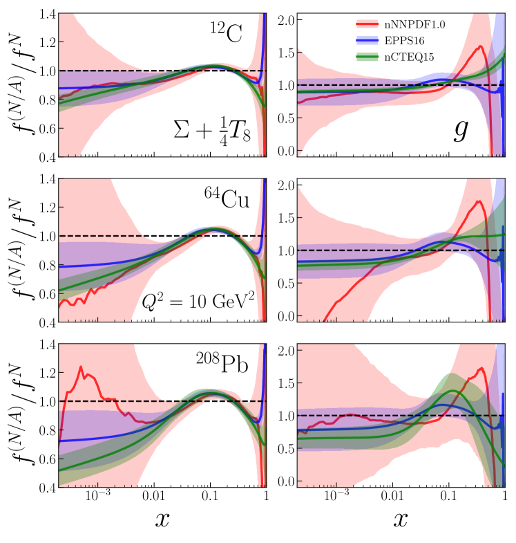
From this comparison, there are a number of interesting similarities and differences between the three nPDF fits. First of all, the three nuclear regimes sketched in Fig. 5.1, namely shadowing, anti-shadowing, and the EMC effect, are visible between the three sets for the quark combination . Interestingly, in the data region the PDF uncertainties for this quark combination are similar between the different analyses. Much larger differences are found in the small- and large- extrapolation regions, particularly for nCTEQ15, where the uncertainties are smaller. Note that the different approaches for uncertainty estimation have noticeable physical consequences. For instance, it would appear that there is rather strong evidence for quark shadowing down to for the nCTEQ15 result, while for nNNPDF1.0, the nuclear modifications are consistent with zero within uncertainties for .
Concerning the nuclear modifications of the gluon PDF, here we can percieve large differences at the level of PDF errors, with nCTEQ15 exhibiting the smallest uncertainties and nNNPDF1.0 the largest. While nCTEQ15 indicates some evidence of small- gluon shadowing, this evidence is absent from both nNNPDF1.0 and EPPS16. Moreover, the three sets find some preference for a mild enhancement of the gluon at large , but the PDF uncertainties prevent making any definite statement. Overall, the various analyses agree well within the large uncertainties for .
While it is beyond the scope of this paper to pin down the origin of the differences between the three nPDF analyses, one known reason is the choice of nPDF parameterization together with the method of imposing the boundary condition. Recall that in nNNPDF1.0 we adopt a model-independent parameterization based on neural networks, Eq. (3.2), with the boundary condition imposed at the optimization level in Eq. (3.2). In the EPPS16 analysis, the bound nucleus PDFs are instead defined relative to a free nucleon baseline (CT14) as
| (5.5) |
where the nuclear modification factors are parameterized at the input evolution scale with piece-wise polynomials that hard-wire some of the theoretical expectations shown in Fig. 5.1. In this approach, the information contained in PDF uncertainties of the free nucleon baseline is not exploited to constrain the nPDFs.
In the nCTEQ15 analysis, the nuclear PDFs are parameterized by a polynomial functional form given by
| (5.6) |
where the coefficients encode all the dependence. During the fit, these coefficients are constrained in a way that for they reproduce the central value of the the CTEQ6.1-like fit of Ref. [100]. Note here that in the nCTEQ15 fit the baseline proton set does not include the experimental measurements that have become available in the last decade, in particular the information provided by the high-precision LHC data and the HERA combined structure functions. Moreover, as in the case of EPPS16, the information about the PDF uncertainties in the free-nucleon case is not exploited to constrain the nPDF errors.
Perturbative stability.
To conclude the discussion of the main properties of the nNNPDF1.0 fits, in Fig. 5.9 we compare the NLO and NNLO nuclear ratios for the same three nuclei as in Fig. 5.8. The ratios are constructed using the distributions from their respective perturbative order PDF set using replicas. In terms of central values, we can see that the NLO and NNLO fit results are consistent within the 90% CL uncertainty band. The regions where the differences between the two perturbative orders are the largest turn out to be the small- and large- extrapolation regions, in particular as is increased.
Another difference between the NLO and NNLO nNNPDF1.0 fits concerns the size of the PDF uncertainty band. We find that for the gluon nPDF, the NNLO fit leads to a slight decrease in uncertainties, perhaps due to the improved overall fit consistency when higher-order theoretical calculations are used. This effect is more distinct for the gluon distribution of and nuclei, while it is mostly absent for . The apparent reduction of uncertainties, together with marginally better values (see Table 5.1), suggests that the NNLO fit is only slightly preferred over the NLO one. That said, the difference is unlikely to have significant phenomenological implications given the current level of uncertainties.
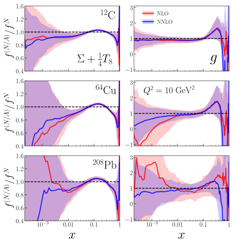
5.3 Methodological studies
We conclude the discussion of the nNNPDF1.0 results by presenting some further studies that demonstrate the robustness of our fitting methodology, complementing those based on the closure tests discussed in Sect. 4. In particular, in the following we discuss the stability of our results with respect to variations of the neural network architecture and the role of the boundary condition in constraining the nPDF uncertainties. For all results presented in this section, we use Monte Carlo replicas.
Stability with respect to the network architecture.
As explained in Sect. 3.1, the nNNPDF1.0 fits are based on a single neural network with the 3-25-3 architecture represented in Fig. 3.2. This architecture is characterized by free parameters, without counting the preprocessing exponents. We have verified that this choice of network architecture is redundant given our input dataset, namely that the nNNPDF1.0 results are stable if neurons are either added or removed from the hidden layer of the network. To illustrate this redundancy, here we compare fit results using the standard 3-25-3 architecture with that using twice as many neurons in the hidden layer, 3-50-3. The latter configuration is characterized by free parameters, which is enlarged by a factor two compared to the baseline fits.
In Fig. 5.10 the nNNPDF1.0 results at the input scale GeV for 12C and 208Pb nuclei are shown with the two different architectures, 3-25-3 (baseline) and 3-50-3. We find that differences are very small and consistent with statistical fluctuations. Given that now there are twice as many free parameters as in the baseline settings, this stability demonstrates that our results are driven by the input experimental data and not by methodological choices such as the specific network architecture. Furthermore, we have also verified that the outcome of the fits is similarly unchanged if a network architecture with a comparable number of parameters but two hidden layers is used.
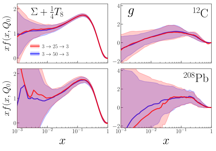
The role of the boundary condition.
Imposing the boundary condition Eq. (3.8) leads to important constraints on both the central values and the uncertainties of nNNPDF1.0 fit, particularly for low values of the atomic mass number . Here we want to quantify this impact by comparing the baseline nNNPDF1.0 results with those of the corresponding fit where this boundary condition has not been imposed. This can be achieved by performing the fits with the hyper-parameter in Eq. (3.2). Note that in this case the behavior of the fitted at nPDFs for is unconstrained, since only experimental data with is included in the fit.
In Fig. 5.11, we show a comparison between the nNNPDF1.0 baseline, which imposes NNPDF3.1 as the boundary condition between and , in addition to a resulting fit where this boundary condition is not implemented. Moreover, we display the gluon and the quark combination at GeV2 for and 64. This comparison demonstrates a significant impact on nNNPDF1.0 resulting from the constraint, especially for helium and carbon nuclei where the PDF uncertainties are increased dramatically if no boundary condition is used. The impact is more distinct for the gluon, where even for relatively heavy nuclei such as 64Cu the boundary condition leads to a reduction of the nPDF uncertainties by up to a factor two. We can thus conclude that imposing consistently the limit using a state-of-the-art proton fit is an essential ingredient of any nPDF analysis.
While the baseline nNNPDF1.0 fits only constrain the distribution between and , one in principle could extend the coverage of the boundary condition down to smaller values of provided a reliable proton PDF baseline is used. Indeed, it is possible to demonstrate that we can impose the constraint down to much smaller values of , e.g. . For this purpose, we perform a fit using instead for the boundary condition the NNPDF3.0+LHCb NLO sets constructed in Ref. [89, 90]. More specifically we use the set based on the , , and normalized distributions of meson production in the forward region at 5, 7, and 13 TeV. The reason is that these sets exhibit reduced quark and gluon PDF uncertainties down to , and therefore are suitable to constrain the small- nPDF uncertainties.
The comparison between the baseline nNNPDF1.0 fit and its LHCb variant is shown in Fig. 5.11. We now find a further reduction of the nPDF uncertainties at small-, again more notably for light nuclei. In this case, the reduction of uncertainties is more distinct for the quarks, which benefit from the very accurate determination of the proton’s quark sea at small- in NNPDF3.0+LHCb. Note that, in turn, the improved nPDF errors at small- might lead to increased sensitivity to effects such as shadowing and evidence for non-linear evolution corrections.
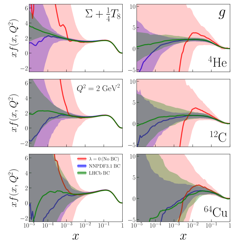
6 Nuclear PDFs at the Electron-Ion Collider
As illustrated by Fig. 2.1, the kinematic reach in is rather limited for the available lepton-nucleus deep-inelastic scattering data. As a consequence, nPDF analyses based on these measurements will exhibit large uncertainties for , as was shown in Sect. 5. However, the coverage at small and large can be improved with measurements in proton-ion scattering, in particular from the p+Pb collisions provided by the LHC. There, small- gluon shadowing can be studied with meson production [105] and direct photon production [106, 107] in the forward region. Furthermore, quark-flavor separation at can be disentangled using the rapidity distributions in and production [31]. On the other hand, access to these extended kinematic regions is desirable also with lepton-nucleus scattering, since leptons represent significantly cleaner probes in scattering processes, as was extensively demonstrated by the HERA collider [108].
Such a machine would be realized by an Electron-Ion Collider (EIC) [109, 110], currently under active discussion in the U.S. The EIC would collide electrons with protons and nuclei using a range of different beam energy configurations and nucleon species, pinning down nuclear modifications of the free-nucleon PDFs down to . Such a machine would therefore significantly improve our understanding of the strong interaction in the nuclear medium, in a similar way as it would with the spin structure of the nucleons [111, 112, 113]. Another option in discussion is the Large Hadron electron Collider (LHeC) [114], which would operate concurrently with the High-Luminosity LHC and would further extend the low- coverage of lepton-nucleus reactions down to . Both options for future high-energy lepton-nucleus colliders have demonstrated their potential to constrain the nuclear PDFs [115, 116, 13].
In this section, we quantify the constraints that future EIC measurements of inclusive nuclear structure functions would impose on the nNNPDF1.0 nuclear PDFs. To achieve this, we generate EIC pseudo-data following Ref. [13], where it was subsequently interpreted in the framework of the EPPS16 analysis of nPDFs. The projections used here are constructed instead with the central value of the nNNPDF1.0 NLO set for different scenarios of the lepton and nucleon beam energies, which are then added to the input data of this analysis listed in Table 2.1 .
The simulated EIC pseudo-data from Ref. [13] is available for both carbon ( and ) and gold ( and ) nuclei. We assume that the latter would be corrected for non-isoscalarity effects, and therefore treat gold as an isoscalar nucleus with (see also Sect. 2). The nuclear structure functions for carbon and gold nuclei are then normalized by the deuteron structure functions following Eq. (2.5).
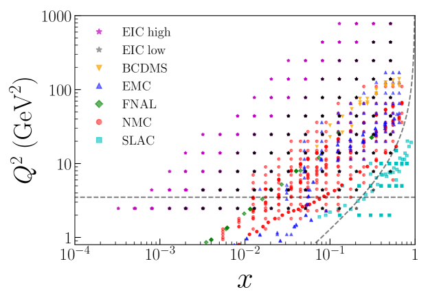
The different scenarios for the lepton and nucleon beam energies of the EIC pseudo-data that are considered here are listed in Table 6.1. As in Ref. [13], we denote the “low energy” EIC scenario the one that consists of measurements taken with electron beams with energy GeV, whereas the “high energy” EIC scenario corresponds to measurements taken with GeV electrons. We also indicate in Table 6.1 the atomic mass number , the nucleus (per nucleon) energy, the maximum and minimum values of and of the pseudo-data, respectively, and the number of pseudo-data points . Here we restrict ourselves again to the inclusive structure functions and do not include EIC pseudo-data on charm structure functions.
| Scenario | ||||||
|---|---|---|---|---|---|---|
| eRHIC_5x50C | 12 | 5 GeV | 50 GeV | 440 GeV2 | 0.003 | 50 |
| eRHIC_5x75C | 12 | 5 GeV | 75 GeV | 440 GeV2 | 0.002 | 57 |
| eRHIC_5x100C | 12 | 5 GeV | 100 GeV | 780 GeV2 | 0.001 | 64 |
| eRHIC_5x50Au | 197 | 5 GeV | 50 GeV | 440 GeV2 | 0.003 | 50 |
| eRHIC_5x75Au | 197 | 5 GeV | 75 GeV | 440 GeV2 | 0.002 | 57 |
| eRHIC_5x100Au | 197 | 5 GeV | 100 GeV | 780 GeV2 | 0.001 | 64 |
| eRHIC_20x50C | 12 | 20 GeV | 50 GeV | 780 GeV2 | 0.0008 | 75 |
| eRHIC_20x75C | 12 | 20 GeV | 75 GeV | 780 GeV2 | 0.0005 | 79 |
| eRHIC_20x100C | 12 | 20 GeV | 100 GeV | 780 GeV2 | 0.0003 | 82 |
| eRHIC_20x50Au | 197 | 20 GeV | 50 GeV | 780 GeV2 | 0.0008 | 75 |
| eRHIC_20x75Au | 197 | 20 GeV | 75 GeV | 780 GeV2 | 0.0005 | 79 |
| eRHIC_20x100Au | 197 | 20 GeV | 100 GeV | 780 GeV2 | 0.0003 | 82 |
In Fig. 6.1, we display the kinematic coverage of the EIC pseudo-data compared to the existing lepton-nucleus scattering measurements. Here we can see that the EIC would significantly extend the sensitivity to nPDFs both in the small- and in the large- regions. This is particularly marked for the higher energy scenario with GeV and GeV, where the kinematic coverage at small in the perturbative region GeV would be increased by a factor 20.
In this exercise, we assume that the “true” central value of the EIC pseudo-data is the central value of the nNNPDF1.0 NLO fit, which is then fluctuated according to the corresponding experimental uncertainties. Given that we also use NLO QCD theory for the fits including EIC data, by construction the resulting fits are expected to have . Concerning the projected experimental uncertainties for the EIC pseudo-data, we assume the same total relative uncertainty as in Ref. [115], which is taken to be uncorrelated among different bins. Moreover, each of the scenarios listed in Table 6.1 are assumed to have a normalization uncertainty, not included in the total uncertainty mentioned above. This normalization error is taken to be fully correlated among each scenario but uncorrelated among the different scenarios. Note that the different nucleus energies in Table 6.1 are statistically independent, so they can be added simultaneously to the same nPDF fit without any double counting.
The results of the fits are given in Fig. 6.2, where a comparison between the nNNPDF1.0 NLO fit and the corresponding fit including the different EIC pseudo-dataset scenarios is shown. We show results at GeV2 for 12C and 197Au, the two nuclei for which pseudo-data is available. Since by construction the central values of the nNNPDF1.0 and nNNPDF1.0+EIC fits will coincide, the most pertinent information is the relative reduction of the nPDF uncertainties. In all cases, we have verified that is obtained.
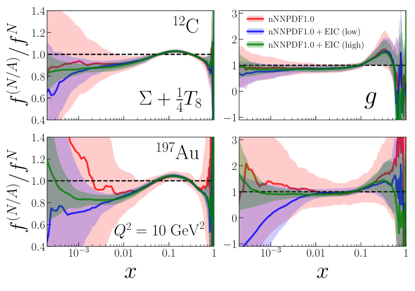
From the comparisons in Fig. 6.2, one finds that the EIC measurements would lead to a significant reduction in the PDF uncertainties both for the gluon and for the quark combination. The effect is especially visible for gold (), given that the constraint from the proton boundary condition is much smaller there than for a lighter nuclei such as carbon (). Here, the improvement can be up to an order of magnitude for as compared to the current situation. Therefore it is clear that such improvement will allow the EIC to carefully study important dynamics such as the quark and gluon shadowing in addition to the possible onset of saturation effects down to .
From Fig. 6.2 we can also observe that the “high energy” scenario would constrain the nPDFs down to smaller values of better than the “low energy” one, again more notably for heavier nuclei such as gold. For instance, the uncertainty for the gluon distribution in the region would be around three times larger in the lower energy case compared to the higher scenario. Given that saturation effects are expected to scale by , these results demonstrate that the “high energy” scenario would provide a rather sharper probe of small- QCD dynamics that the lower energy option.
7 Summary and outlook
In this work, we have presented a first determination of the parton distribution functions of nucleons bound within nuclei using the NNPDF methodology. Using as experimental input all available measurements on neutral-current deep-inelastic nuclear structure functions, we have determined the nuclear gluon , the quark singlet , and the quark octet for a range of atomic mass numbers from to . We find an excellent overall agreement with the fitted experimental data, with stable results with respect to the order of the perturbative QCD calculations. While the quark distributions are reasonably well constrained for , the nuclear gluon PDFs are affected by large uncertainties, in particular for heavy nuclei.
From the methodological point of view, the main improvement with respect to previous NNPDF fits has been the implementation of TensorFlow to perform stochastic gradient descent with reverse-mode automatic differentiation. The application of SGD for the minimization has lead to a marked performance improvement as compared to the evolutionary-type algorithms used so far in NNPDF. Two other related developments in this study have been the use of a single neutral network to parameterize the nPDFs rather than multiple networks, and the fitting of the preprocessing exponents rather than their determination from an iterative procedure.
As opposed to other nPDF analyses, the nNNPDF1.0 set is determined with the boundary condition imposed at the minimization level so that the baseline proton PDFs (NNPDF3.1) are reproduced both in terms of their central values and, more importantly, their uncertainties. Moreover, we have applied this constraint in a fully consistent way, since the proton PDF baseline has been determined using the same fitting methodology and theoretical settings. We have shown that this constraint results in a significant reduction of the nPDF uncertainties, especially for low- nuclei, and therefore represents a vital ingredient for any nPDF analysis.
By using nNNPDF1.0 as a baseline, we have also quantified the impact of future e+A measurements from an Electron-Ion Collider by exploiting the projections generated in Ref. [13]. We have demonstrated that the EIC measurements of inclusive nuclear structure functions would constrain the quark and gluon nuclear PDFs down to , opening a new window to study the nuclear modification of the proton substructure in the small- region. With future EIC measurments, it will therefore be possible to construct a reliable nPDF set based on collinear factorization that can identify and isolate the onset of novel QCD regimes such as non-linear evolution effects or small- resummation.
The main limitations of the present work are the lack of a reliable separation between the quark flavors, which is not possible from neutral-current DIS measurements alone, as well as the large uncertainties that affect the nuclear gluon PDFs. This implies that the possible phenomenological applications of nNNPDF1.0 are restricted to processes that do not require a complete quark flavor separation, such as the analysis of EIC structure functions in Sect. 6, or meson production in p+Pb collisions [105]. To bypass these limitations, we plan to extend the present nPDF analysis to a global dataset including neutrino-induced charged-current deep-inelastic structure functions as well as inclusive jets and dijets, photons, electroweak boson production, and heavy quark production from proton-ion collisions from RHIC and the LHC.
The results of this work, namely the nNNPDF1.0 NLO and NNLO sets for different values of , are available via the LHAPDF library [117], and have also been linked to the NNPDF website:
http://nnpdf.mi.infn.it/for-users/nuclear-pdf-sets/
These LHAPDF grid files contains replicas each, which are fully correlated between different values of as discussed in Sect. 5.
Moreover, due to the lack of a complete quark flavour separation, additional assumptions might be required when the nNNPDF1.0 sets are used, in particular for phenomenological applications in heavy-ion collisions. To comply with the LHAPDF format, we have assumed that and that , namely a symmetric quark sea. With this convention, the only meaningfully constrained quark combinations can be reconstructed using the flavour basis PDFs by means of and .
Acknowledgements
We are grateful to our colleagues of the NNPDF collaboration for illuminating discussions. We thank Nathan Hartland and Carlota Andrés Casas for collaboration in the initial stages of this work. We are grateful to Alexander Kusina and Hannu Paukkunen for information about the nCTEQ15 and EPPS16 nuclear sets. We thank Hannu Paukkunen and Pia Zurita for sharing with us their projections for the EIC pseudo-data. J. R. is partially supported by the European Research Council Starting Grant “PDF4BSM”. R. A..K., J. E., and J. R. are supported by the Netherlands Organization for Scientific Research (NWO).
References
- [1] European Muon Collaboration, J. J. Aubert et al., The ratio of the nucleon structure functions for iron and deuterium, Phys. Lett. 123B (1983) 275–278.
- [2] P. Zurita, Recent progress in Nuclear Parton Distributions, in 13th Conference on the Intersections of Particle and Nuclear Physics (CIPANP 2018) Palm Springs, California, USA, May 29-June 3, 2018, 2018. arXiv:1810.00099.
- [3] H. Paukkunen, Nuclear PDFs Today, in 9th International Conference on Hard and Electromagnetic Probes of High-Energy Nuclear Collisions: Hard Probes 2018 (HP2018) Aix-Les-Bains, Savoie, France, October 1-5, 2018, 2018. arXiv:1811.01976.
- [4] J. Gao, L. Harland-Lang, and J. Rojo, The Structure of the Proton in the LHC Precision Era, Phys. Rept. 742 (2018) 1–121, [arXiv:1709.04922].
- [5] N. Armesto, N. Borghini, S. Jeon, U. A. Wiedemann, S. Abreu, V. Akkelin, J. Alam, J. L. Albacete, A. Andronic, D. Antonov, et al., Heavy Ion Collisions at the LHC - Last Call for Predictions, J. Phys. G35 (2008) 054001, [arXiv:0711.0974].
- [6] STAR Collaboration, J. Adams et al., Experimental and theoretical challenges in the search for the quark gluon plasma: The STAR Collaboration’s critical assessment of the evidence from RHIC collisions, Nucl. Phys. A757 (2005) 102–183, [nucl-ex/0501009].
- [7] NNPDF Collaboration, R. D. Ball et al., Parton distributions for the LHC Run II, JHEP 04 (2015) 040, [arXiv:1410.8849].
- [8] S. Dulat, T.-J. Hou, J. Gao, M. Guzzi, J. Huston, P. Nadolsky, J. Pumplin, C. Schmidt, D. Stump, and C. P. Yuan, New parton distribution functions from a global analysis of quantum chromodynamics, Phys. Rev. D93 (2016), no. 3 033006, [arXiv:1506.07443].
- [9] L. A. Harland-Lang, A. D. Martin, P. Motylinski, and R. S. Thorne, Parton distributions in the LHC era: MMHT 2014 PDFs, Eur. Phys. J. C75 (2015) 204, [arXiv:1412.3989].
- [10] S. Alekhin, J. Blümlein, S. Moch, and R. Placakyte, Parton distribution functions, , and heavy-quark masses for LHC Run II, Phys. Rev. D96 (2017), no. 1 014011, [arXiv:1701.05838].
- [11] NNPDF Collaboration, R. D. Ball, E. R. Nocera, and R. L. Pearson, Nuclear Uncertainties in the Determination of Proton PDFs, arXiv:1812.09074.
- [12] The NNPDF Collaboration, R. D. Ball et al., Precision determination of electroweak parameters and the strange content of the proton from neutrino deep-inelastic scattering, Nucl. Phys. B823 (2009) 195–233, [arXiv:0906.1958].
- [13] E. C. Aschenauer, S. Fazio, M. A. C. Lamont, H. Paukkunen, and P. Zurita, Nuclear Structure Functions at a Future Electron-Ion Collider, Phys. Rev. D96 (2017), no. 11 114005, [arXiv:1708.05654].
- [14] LHeC Study Group Collaboration, J. Abelleira Fernandez et al., A Large Hadron Electron Collider at CERN: Report on the Physics and Design Concepts for Machine and Detector, J.Phys. G39 (2012) 075001, [arXiv:1206.2913].
- [15] I. Helenius, H. Paukkunen, and N. Armesto, nPDF constraints from the Large Hadron Electron Collider, in Proceedings, 24th International Workshop on Deep-Inelastic Scattering and Related Subjects (DIS 2016): Hamburg, Germany, April 11-25, 2016, 2016. arXiv:1606.09003.
- [16] R. D. Ball, V. Bertone, M. Bonvini, S. Marzani, J. Rojo, and L. Rottoli, Parton distributions with small-x resummation: evidence for BFKL dynamics in HERA data, Eur. Phys. J. C78 (2018), no. 4 321, [arXiv:1710.05935].
- [17] K. J. Eskola, H. Paukkunen, and C. A. Salgado, EPS09 - a New Generation of NLO and LO Nuclear Parton Distribution Functions, arXiv:0902.4154.
- [18] D. de Florian and R. Sassot, Nuclear parton distributions at next to leading order, Phys. Rev. D69 (2004) 074028, [hep-ph/0311227].
- [19] M. Hirai, S. Kumano, and T. H. Nagai, Determination of nuclear parton distribution functions and their uncertainties at next-to-leading order, Phys. Rev. C76 (2007) 065207, [arXiv:0709.3038].
- [20] K. Kovarik et al., nCTEQ15 - Global analysis of nuclear parton distributions with uncertainties in the CTEQ framework, Phys. Rev. D93 (2016), no. 8 085037, [arXiv:1509.00792].
- [21] D. de Florian, R. Sassot, P. Zurita, and M. Stratmann, Global Analysis of Nuclear Parton Distributions, Phys. Rev. D85 (2012) 074028, [arXiv:1112.6324].
- [22] H. Khanpour and S. Atashbar Tehrani, Global Analysis of Nuclear Parton Distribution Functions and Their Uncertainties at Next-to-Next-to-Leading Order, Phys. Rev. D93 (2016), no. 1 014026, [arXiv:1601.00939].
- [23] ALICE Collaboration, J. Adam et al., Measurement of charged jet production cross sections and nuclear modification in p-Pb collisions at TeV, Phys. Lett. B749 (2015) 68–81, [arXiv:1503.00681].
- [24] ALICE Collaboration, J. Adam et al., Multiplicity dependence of charged pion, kaon, and (anti)proton production at large transverse momentum in p-Pb collisions at = 5.02 TeV, Phys. Lett. B760 (2016) 720–735, [arXiv:1601.03658].
- [25] ALICE Collaboration, J. Adam et al., Measurement of dijet in p–Pb collisions at =5.02 TeV, Phys. Lett. B746 (2015) 385–395, [arXiv:1503.03050].
- [26] ATLAS Collaboration, G. Aad et al., Transverse momentum, rapidity, and centrality dependence of inclusive charged-particle production in TeV p+Pb collisions measured by the ATLAS experiment, arXiv:1605.06436.
- [27] CMS Collaboration, S. Chatrchyan et al., Studies of dijet transverse momentum balance and pseudorapidity distributions in pPb collisions at TeV, Eur. Phys. J. C74 (2014), no. 7 2951, [arXiv:1401.4433].
- [28] ALICE Collaboration, J. Zhu, Measurement of w-boson production in p–pb collisions at = 5.02 tev with alice at the lhc, Journal of Physics: Conference Series 612 (2015), no. 1 012009.
- [29] ATLAS Collaboration, G. Aad et al., Measurement of production in +Pb collision at TeV with ATLAS detector at the LHC, ATLAS-CONF-2015-056.
- [30] ATLAS Collaboration, G. Aad et al., boson production in Pb collisions at TeV measured with the ATLAS detector, Phys. Rev. C92 (2015), no. 4 044915, [arXiv:1507.06232].
- [31] CMS Collaboration, V. Khachatryan et al., Study of Z boson production in pPb collisions at =5.02TeV, Phys. Lett. B759 (2016) 36–57, [arXiv:1512.06461].
- [32] CMS Collaboration, V. Khachatryan et al., Study of W boson production in pPb collisions at 5.02 TeV, Phys. Lett. B750 (2015) 565–586, [arXiv:1503.05825].
- [33] CMS Collaboration, S. Chatrchyan et al., Charm-tagged jet production in pPb collisions at 5.02 TeV and pp collisions at 2.76 TeV, CMS-PAS-HIN-15-012.
- [34] ALICE Collaboration, J. Adam et al., Measurement of D-meson production versus multiplicity in p-Pb collisions at TeV, JHEP 08 (2016) 078, [arXiv:1602.07240].
- [35] ALICE Collaboration, J. Adam et al., Measurement of electrons from heavy-flavour hadron decays in p-Pb collisions at 5.02 TeV, Phys. Lett. B754 (2016) 81–93, [arXiv:1509.07491].
- [36] ALICE Collaboration, B. B. Abelev et al., Measurement of prompt -meson production in collisions at = 5.02 TeV, Phys. Rev. Lett. 113 (2014), no. 23 232301, [arXiv:1405.3452].
- [37] CMS Collaboration, V. Khachatryan et al., Transverse momentum spectra of inclusive b jets in pPb collisions at 5.02 TeV, Phys. Lett. B754 (2016) 59, [arXiv:1510.03373].
- [38] CMS Collaboration, V. Khachatryan et al., Study of B Meson Production in pPb Collisions at 5.02 TeV Using Exclusive Hadronic Decays, Phys. Rev. Lett. 116 (2016), no. 3 032301, [arXiv:1508.06678].
- [39] LHCb Collaboration, R. Aaij et al., Study of prompt D0 meson production in Pb collisions at TeV, JHEP 10 (2017) 090, [arXiv:1707.02750].
- [40] LHCb Collaboration, R. Aaij et al., Measurement of , and production in collisions at , Phys. Rev. D99 (2019), no. 5 052011, [arXiv:1902.05599].
- [41] K. J. Eskola, P. Paakkinen, H. Paukkunen, and C. A. Salgado, EPPS16: Nuclear parton distributions with LHC data, Eur. Phys. J. C77 (2017), no. 3 163, [arXiv:1612.05741].
- [42] A. Kusina, F. Lyonnet, D. B. Clark, E. Godat, T. Jezo, K. Kovarik, F. I. Olness, I. Schienbein, and J. Y. Yu, Vector boson production in pPb and PbPb collisions at the LHC and its impact on nCTEQ15 PDFs, Eur. Phys. J. C77 (2017), no. 7 488, [arXiv:1610.02925].
- [43] S. Forte, L. Garrido, J. I. Latorre, and A. Piccione, Neural network parametrization of deep-inelastic structure functions, JHEP 05 (2002) 062, [hep-ph/0204232].
- [44] The NNPDF Collaboration, L. Del Debbio, S. Forte, J. I. Latorre, A. Piccione, and J. Rojo, Unbiased determination of the proton structure function f2(p) with estimation, JHEP 03 (2005) 080, [hep-ph/0501067].
- [45] The NNPDF Collaboration, L. Del Debbio, S. Forte, J. I. Latorre, A. Piccione, and J. Rojo, Neural network determination of parton distributions: The nonsinglet case, JHEP 03 (2007) 039, [hep-ph/0701127].
- [46] The NNPDF Collaboration, R. D. Ball et al., A determination of parton distributions with faithful uncertainty estimation, Nucl. Phys. B809 (2009) 1–63, [arXiv:0808.1231].
- [47] The NNPDF Collaboration, J. Rojo et al., Update on Neural Network Parton Distributions: NNPDF1.1, arXiv:0811.2288.
- [48] The NNPDF Collaboration, R. D. Ball et al., Fitting Parton Distribution Data with Multiplicative Normalization Uncertainties, JHEP 05 (2010) 075, [arXiv:0912.2276].
- [49] The NNPDF Collaboration, R. D. Ball et al., A first unbiased global NLO determination of parton distributions and their uncertainties, Nucl. Phys. B838 (2010) 136, [arXiv:1002.4407].
- [50] The NNPDF Collaboration, R. D. Ball et al., Impact of Heavy Quark Masses on Parton Distributions and LHC Phenomenology, Nucl. Phys. B849 (2011) 296, [arXiv:1101.1300].
- [51] The NNPDF Collaboration, R. D. Ball et al., Unbiased global determination of parton distributions and their uncertainties at NNLO and at LO, Nucl.Phys. B855 (2012) 153, [arXiv:1107.2652].
- [52] R. D. Ball et al., Parton distributions with LHC data, Nucl.Phys. B867 (2013) 244, [arXiv:1207.1303].
- [53] S. Forte, E. Laenen, P. Nason, and J. Rojo, Heavy quarks in deep-inelastic scattering, Nucl. Phys. B834 (2010) 116–162, [arXiv:1001.2312].
- [54] M. Abadi et al., TensorFlow: Large-scale machine learning on heterogeneous systems, 2015. Software available from tensorflow.org.
- [55] European Muon Collaboration, J. J. Aubert et al., Measurements of the nucleon structure functions in deep inelastic muon scattering from deuterium and comparison with those from hydrogen and iron, Nucl. Phys. B293 (1987) 740–786.
- [56] European Muon Collaboration, J. Ashman et al., Measurement of the Ratios of Deep Inelastic Muon - Nucleus Cross-Sections on Various Nuclei Compared to Deuterium, Phys. Lett. B202 (1988) 603–610.
- [57] European Muon Collaboration, M. Arneodo et al., Measurements of the nucleon structure function in the range and in deuterium, carbon and calcium, Nucl. Phys. B333 (1990) 1–47.
- [58] European Muon Collaboration, J. Ashman et al., A Measurement of the ratio of the nucleon structure function in copper and deuterium, Z.Phys. C57 (1993) 211–218.
- [59] New Muon Collaboration, P. Amaudruz et al., A Reevaluation of the nuclear structure function ratios for D, He, Li-6, C and Ca, Nucl.Phys. B441 (1995) 3–11, [hep-ph/9503291].
- [60] New Muon Collaboration, M. Arneodo et al., The Structure Function ratios F2(li) / F2(D) and F2(C) / F2(D) at small x, Nucl.Phys. B441 (1995) 12–30, [hep-ex/9504002].
- [61] New Muon Collaboration, M. Arneodo et al., The A dependence of the nuclear structure function ratios, Nucl.Phys. B481 (1996) 3–22.
- [62] New Muon Collaboration, M. Arneodo et al., The dependence of the structure function ratio in deep inelastic muon scattering, Nucl.Phys. B481 (1996) 23–39.
- [63] J. Gomez et al., Measurement of the dependence of deep-inelastic electron scattering, Phys. Rev. D49 (1994) 4348.
- [64] New Muon Collaboration, P. Amaudruz et al., Measurements of R(d) - R(p) and R(Ca) - R(C) in deep inelastic muon scattering, Phys. Lett. B294 (1992) 120–126.
- [65] S. Dasu et al., Measurement of the Difference in R = l / t and (a) / ) in Deep Inelastic , Fe and Au Scattering, Phys. Rev. Lett. 60 (1988) 2591.
- [66] J. Gomez et al., Measurement of the A-dependence of deep inelastic electron scattering, Phys. Rev. D49 (1994) 4348–4372.
- [67] E665 Collaboration, M. R. Adams et al., Shadowing in inelastic scattering of muons on carbon, calcium and lead at low x(Bj), Z. Phys. C67 (1995) 403–410, [hep-ex/9505006].
- [68] D. M. Alde et al., Nuclear dependence of dimuon production at 800-GeV. FNAL-772 experiment, Phys. Rev. Lett. 64 (1990) 2479–2482.
- [69] BCDMS Collaboration, A. C. Benvenuti et al., Nuclear Effects in Deep Inelastic Muon Scattering on Deuterium and Iron Targets, Phys. Lett. B189 (1987) 483–487.
- [70] Fermilab E665 Collaboration, M. R. Adams et al., Shadowing in the muon xenon inelastic scattering cross-section at 490-GeV, Phys. Lett. B287 (1992) 375–380.
- [71] NNPDF Collaboration, R. D. Ball et al., Parton distributions from high-precision collider data, Eur. Phys. J. C77 (2017), no. 10 663, [arXiv:1706.00428].
- [72] G. D’Agostini, Bayesian reasoning in data analysis: A critical introduction. World Scientific, 2003.
- [73] L. Del Debbio, N. P. Hartland, and S. Schumann, MCgrid: projecting cross section calculations on grids, Comput.Phys.Commun. 185 (2014) 2115–2126, [arXiv:1312.4460].
- [74] V. Bertone, R. Frederix, S. Frixione, J. Rojo, and M. Sutton, aMCfast: automation of fast NLO computations for PDF fits, JHEP 1408 (2014) 166, [arXiv:1406.7693].
- [75] T. Carli et al., A posteriori inclusion of parton density functions in NLO QCD final-state calculations at hadron colliders: The APPLGRID Project, Eur.Phys.J. C66 (2010) 503, [arXiv:0911.2985].
- [76] fastNLO Collaboration, M. Wobisch, D. Britzger, T. Kluge, K. Rabbertz, and F. Stober, Theory-Data Comparisons for Jet Measurements in Hadron-Induced Processes, arXiv:1109.1310.
- [77] V. Bertone, S. Carrazza, and N. P. Hartland, APFELgrid: a high performance tool for parton density determinations, Comput. Phys. Commun. 212 (2017) 205–209, [arXiv:1605.02070].
- [78] V. Bertone, S. Carrazza, and J. Rojo, APFEL: A PDF Evolution Library with QED corrections, Comput.Phys.Commun. 185 (2014) 1647, [arXiv:1310.1394].
- [79] Particle Data Group Collaboration, M. Tanabashi et al., Review of Particle Physics, Phys. Rev. D98 (2018), no. 3 030001.
- [80] NNPDF Collaboration, R. D. Ball, S. Carrazza, L. Del Debbio, S. Forte, Z. Kassabov, J. Rojo, E. Slade, and M. Ubiali, Precision determination of the strong coupling constant within a global PDF analysis, Eur. Phys. J. C78 (2018), no. 5 408, [arXiv:1802.03398].
- [81] A. Verbytskyi, A. Banfi, A. Kardos, P. F. Monni, S. Kluth, G. Somogyi, Z. Szőr, Z. Trócsányi, Z. Tulipánt, and G. Zanderighi, High precision determination of from a global fit of jet rates, arXiv:1902.08158.
- [82] ALPHA Collaboration, M. Bruno, M. Dalla Brida, P. Fritzsch, T. Korzec, A. Ramos, S. Schaefer, H. Simma, S. Sint, and R. Sommer, QCD Coupling from a Nonperturbative Determination of the Three-Flavor Parameter, Phys. Rev. Lett. 119 (2017), no. 10 102001, [arXiv:1706.03821].
- [83] S. Zafeiropoulos, P. Boucaud, F. De Soto, J. Rodríguez-Quintero, and J. Segovia, The strong running coupling from the gauge sector of Domain Wall lattice QCD with physical quark masses, Phys. Rev. Lett. 122 (2019), no. 16 162002, [arXiv:1902.08148].
- [84] A. Pich, J. Rojo, R. Sommer, and A. Vairo, Determining the strong coupling: status and challenges, in 13th Conference on Quark Confinement and the Hadron Spectrum (Confinement XIII) Maynooth, Ireland, July 31-August 6, 2018, 2018. arXiv:1811.11801.
- [85] LHC Higgs Cross Section Working Group Collaboration, D. de Florian et al., Handbook of LHC Higgs Cross Sections: 4. Deciphering the Nature of the Higgs Sector, arXiv:1610.07922.
- [86] NNPDF Collaboration, R. D. Ball, V. Bertone, M. Bonvini, S. Carrazza, S. Forte, A. Guffanti, N. P. Hartland, J. Rojo, and L. Rottoli, A Determination of the Charm Content of the Proton, Eur. Phys. J. C76 (2016), no. 11 647, [arXiv:1605.06515].
- [87] H.-W. Lin et al., Parton distributions and lattice QCD calculations: a community white paper, Prog. Part. Nucl. Phys. 100 (2018) 107–160, [arXiv:1711.07916].
- [88] R. D. Ball, E. R. Nocera, and J. Rojo, The asymptotic behaviour of parton distributions at small and large , Eur. Phys. J. C76 (2016), no. 7 383, [arXiv:1604.00024].
- [89] R. Gauld, J. Rojo, L. Rottoli, and J. Talbert, Charm production in the forward region: constraints on the small-x gluon and backgrounds for neutrino astronomy, JHEP 11 (2015) 009, [arXiv:1506.08025].
- [90] R. Gauld and J. Rojo, Precision determination of the small- gluon from charm production at LHCb, Phys. Rev. Lett. 118 (2017), no. 7 072001, [arXiv:1610.09373].
- [91] V. Bertone, R. Gauld, and J. Rojo, Neutrino Telescopes as QCD Microscopes, JHEP 01 (2019) 217, [arXiv:1808.02034].
- [92] X. Glorot and Y. Bengio, Understanding the difficulty of training deep feedforward neural networks, in JMLR W&CP: Proceedings of the Thirteenth International Conference on Artificial Intelligence and Statistics (AISTATS 2010), vol. 9, pp. 249–256, May, 2010.
- [93] NNPDF Collaboration Collaboration, E. R. Nocera, R. D. Ball, S. Forte, G. Ridolfi, and J. Rojo, A first unbiased global determination of polarized PDFs and their uncertainties, Nucl.Phys. B887 (2014) 276, [arXiv:1406.5539].
- [94] NNPDF Collaboration, V. Bertone, N. P. Hartland, E. R. Nocera, J. Rojo, and L. Rottoli, Charged hadron fragmentation functions from collider data, Eur. Phys. J. C78 (2018), no. 8 651, [arXiv:1807.03310].
- [95] J. Rojo, Machine Learning tools for global PDF fits, in 13th Conference on Quark Confinement and the Hadron Spectrum (Confinement XIII) Maynooth, Ireland, July 31-August 6, 2018, 2018. arXiv:1809.04392.
- [96] D. P. Kingma and J. Ba, Adam: A method for stochastic optimization, CoRR abs/1412.6980 (2014) [arXiv:1412.6980].
- [97] R. Abdul Khalek and V. Bertone, Analytical neural network gradients, .
- [98] N. P. Hartland, F. Maltoni, E. R. Nocera, J. Rojo, E. Slade, E. Vryonidou, and C. Zhang, A Monte Carlo global analysis of the Standard Model Effective Field Theory: the top quark sector, arXiv:1901.05965.
- [99] R. D. Ball and S. Forte, Double asymptotic scaling at hera, Phys. Lett. B335 (1994) 77–86, [hep-ph/9405320].
- [100] J. F. Owens et al., The Impact of new neutrino DIS and Drell-Yan data on large-x parton distributions, Phys. Rev. D75 (2007) 054030, [hep-ph/0702159].
- [101] J. Butterworth et al., PDF4LHC recommendations for LHC Run II, J. Phys. G43 (2016) 023001, [arXiv:1510.03865].
- [102] R. D. Ball, S. Carrazza, L. Del Debbio, S. Forte, J. Gao, et al., Parton Distribution Benchmarking with LHC Data, JHEP 1304 (2013) 125, [arXiv:1211.5142].
- [103] M. Botje et al., The PDF4LHC Working Group Interim Recommendations, arXiv:1101.0538.
- [104] S. Alekhin et al., The PDF4LHC Working Group Interim Report, arXiv:1101.0536.
- [105] A. Kusina, J.-P. Lansberg, I. Schienbein, and H.-S. Shao, Gluon Shadowing in Heavy-Flavor Production at the LHC, Phys. Rev. Lett. 121 (2018), no. 5 052004, [arXiv:1712.07024].
- [106] J. M. Campbell, J. Rojo, E. Slade, and C. Williams, Direct photon production and PDF fits reloaded, Eur. Phys. J. C78 (2018), no. 6 470, [arXiv:1802.03021].
- [107] ALICE Collaboration, T. Peitzmann, Forward photon measurements in ALICE as a probe for low-x gluons, in 9th International Conference on Hard and Electromagnetic Probes of High-Energy Nuclear Collisions: Hard Probes 2018 (HP2018) Aix-Les-Bains, Savoie, France, October 1-5, 2018, 2018. arXiv:1812.07246.
- [108] M. Klein and R. Yoshida, Collider Physics at HERA, arXiv:0805.3334.
- [109] A. Accardi et al., Electron Ion Collider: The Next QCD Frontier, Eur. Phys. J. A52 (2016), no. 9 268, [arXiv:1212.1701].
- [110] D. Boer, M. Diehl, R. Milner, R. Venugopalan, W. Vogelsang, et al., Gluons and the quark sea at high energies: Distributions, polarization, tomography, arXiv:1108.1713.
- [111] NNPDF Collaboration, R. D. Ball, S. Forte, A. Guffanti, E. R. Nocera, G. Ridolfi, and J. Rojo, Polarized Parton Distributions at an Electron-Ion Collider, Phys. Lett. B728 (2014) 524–531, [arXiv:1310.0461].
- [112] R. D. Ball and A. Deshpande, The Proton Spin, Semi-Inclusive processes, and a future Electron Ion Collider, 2018. arXiv:1801.04842.
- [113] E. C. Aschenauer, S. Fazio, J. H. Lee, H. Mantysaari, B. S. Page, B. Schenke, T. Ullrich, R. Venugopalan, and P. Zurita, The electron–ion collider: assessing the energy dependence of key measurements, Rept. Prog. Phys. 82 (2019), no. 2 024301, [arXiv:1708.01527].
- [114] J. L. Abelleira Fernandez et al., A Large Hadron Electron Collider at CERN, in CERN Council Open Symposium on European Strategy for Particle Physics (ESPP2012) Cracow, Poland, September 10-12, 2012, 2012. arXiv:1211.4831.
- [115] LHeC study Group Collaboration, H. Paukkunen, An update on nuclear PDFs at the LHeC, PoS DIS2017 (2018) 109, [arXiv:1709.08342].
- [116] I. Helenius, H. Paukkunen, and N. Armesto, Electron-Ion Physics with the LHeC, PoS DIS2015 (2015) 226, [arXiv:1509.02802].
- [117] A. Buckley, J. Ferrando, S. Lloyd, K. Nordström, B. Page, et al., LHAPDF6: parton density access in the LHC precision era, Eur.Phys.J. C75 (2015) 132, [arXiv:1412.7420].