Towards Characterizing Divergence in Deep Q-Learning
Abstract
Deep Q-Learning (DQL), a family of temporal difference algorithms for control, employs three techniques collectively known as the ‘deadly triad’ in reinforcement learning: bootstrapping, off-policy learning, and function approximation. Prior work has demonstrated that together these can lead to divergence in Q-learning algorithms, but the conditions under which divergence occurs are not well-understood. In this note, we give a simple analysis based on a linear approximation to the Q-value updates, which we believe provides insight into divergence under the deadly triad. The central point in our analysis is to consider when the leading order approximation to the deep-Q update is or is not a contraction in the sup norm. Based on this analysis, we develop an algorithm which permits stable deep Q-learning for continuous control without any of the tricks conventionally used (such as target networks, adaptive gradient optimizers, or using multiple Q functions). We demonstrate that our algorithm performs above or near state-of-the-art on standard MuJoCo benchmarks from the OpenAI Gym.
1 Introduction
Deep Q-Learning (DQL), a family of reinforcement learning algorithms that includes Deep Q-Network (DQN) (Mnih et al., 2013, 2015) and its continuous-action variants (Lillicrap et al., 2016; Fujimoto et al., 2018b; Haarnoja et al., 2018b), is often successful at training deep neural networks for control. In DQL, a function approximator (a deep neural network) learns to estimate the value of each state-action pair under the optimal policy (the -function), and a control policy selects actions with the highest values according to the current -function approximator. DQL algorithms have been applied fruitfully in video games (Mnih et al., 2015), robotics (Kalashnikov et al., 2018; Haarnoja et al., 2018a), and user interactions on social media (Gauci et al., 2018).
However, despite the high-profile empirical successes, these algorithms possess failure modes that are poorly understood and arise frequently in practice. The most common failure mode is divergence, where the -function approximator learns to ascribe unrealistically high values to state-action pairs, in turn destroying the quality of the greedy control policy derived from (van Hasselt et al., 2018). Divergence in DQL is often attributed to three components common to all DQL algorithms, which are collectively considered the ‘deadly triad’ of reinforcement learning (Sutton, 1988; Sutton & Barto, 2018):
-
•
function approximation, in this case the use of deep neural networks,
-
•
off-policy learning, the use of data collected on one policy to estimate the value of another policy,
-
•
and bootstrapping, where the -function estimator is regressed towards a function of itself.
Well-known examples (Baird, 1995; Tsitsiklis & Roy, 1997) demonstrate the potential of the deadly triad to cause divergence in approximate -learning. However, actionable descriptions of divergence in the general case remain elusive, prompting algorithm designers to attack the triad with an increasingly wide variety of heuristic solutions. These include target networks (Mnih et al., 2015), entropy regularization (Fox et al., 2016; Haarnoja et al., 2018b), n-step learning (Hessel et al., 2017), and approximate double-Q learning (van Hasselt et al., 2016).
The absence of theoretical characterization for divergence in DQL makes it challenging to reliably deploy DQL on new problems. To make progress toward such a characterization, we give an analysis inspired by Gordon (1995), who studied the behavior of approximate value learning algorithms in value space. We examine how -values change under a standard DQL update, and derive the leading order approximation to the DQL update operator. The approximate update turns out to have a simple form that disentangles and clarifies the contributions from the components of the deadly triad, and allows us to identify the important role played by the neural tangent kernel (NTK) (Jacot et al., 2018) of the approximator. We consider conditions under which the approximate update is or isn’t a contraction map in the sup norm, based on the intuition that when it is a contraction DQL should behave stably, and when it is an expansion we should expect divergence.
Based on our analysis, we design an algorithm which is intended to approximately ensure that the -function update is non-expansive. Our algorithm, which we call Preconditioned Q-Networks (PreQN) is computationally expensive but theoretically simple: it works by preconditioning the TD-errors in minibatch gradient updates, using the inverse of a matrix of inner products of -function gradients. We demonstrate that PreQN is stable and performant on a standard slate of MuJoCo benchmarks from the OpenAI Gym (Brockman et al., 2016), despite using none of the tricks typically associated with DQL. We also find a neat connection between PreQN and natural gradient (Amari, 1998) methods, where under some slightly restricted conditions, the PreQN update is equivalent to a natural gradient Q-learning update. This connection explains a result noted by Knight & Lerner (2018): that natural gradient Q-learning appeared to be stable without target networks.
2 Preliminaries
2.1 Contraction Maps and Fixed Points
We begin with a brief mathematical review. Let be a vector space with norm , and a function from to . If , satisfies
| (1) |
with , then is called a contraction map with modulus . If satisfies Eq 1 but with , then is said to be a non-expansion.
By the Banach fixed-point theorem, if is a contraction, there is a unique fixed-point such that , and it can be obtained by the repeated application of : for any point , if we define a sequence of points such that , .
2.2 Q Functions and TD-Learning
DQL algorithms learn control policies in the reinforcement learning (RL) setting with the infinite-horizon discounted return objective. They attempt to learn an approximator to the optimal action-value function , which is known to satisfy the optimal Bellman equation:
| (2) |
Here, and are states, and are actions, is the transition kernel for the environment, is the reward function, and is the discount factor. The optimal policy can be obtained as the policy which is greedy with respect to : . Thus, DQL algorithms approximate the optimal policy as the policy which is greedy with respect to the -approximator.
Let be the operator on Q functions with given by the RHS of Eq 2; then Eq 2 can be written as . The operator is called the optimal Bellman operator, and it is a contraction in the sup norm with modulus . When the -function can be represented as a finite table and the reward function and transition kernel are fully known, can be computed exactly and can be obtained by value iteration: . The convergence of value iteration from any initial point is guaranteed by the Banach fixed-point theorem.
When the reward function and transition kernel are not fully known, it is still possible to learn in the tabular setting via -learning (Watkins & Dayan, 1992). -learning updates the -values of state-action pairs as they are visited by some exploration policy according to:
| (3) |
where is a sample estimate for using the reward and next state obtained from the environment while exploring. Under mild conditions on state-action visitation (all pairs must be visited often enough) and learning rates (they must all gradually go to zero and always lie in ), -learning converges to . -learning is called a temporal difference (TD) algorithm because the updates to -values are based on the temporal difference error:
3 Towards Characterizing Divergence in Deep Q-Learning
Deep Q-Learning (DQL) algorithms are based on the generalization of Eq 3 to the function approximation setting:
| (4) |
where is a differentiable function approximator with parameters , and are the parameters after an update. Note that when is a table, Eq 4 reduces exactly to Eq 3.
Typically, DQL algorithms make use of experience replay (Lin, 1992) and minibatch gradient descent (Mnih et al., 2013), resulting in an expected update:
| (5) |
where is the distribution of experience in the replay buffer at the time of the update. For stability, it is conventional to replace the bootstrap, the term, with one based on a slowly-updated target network: , where the parameters are either infrequently copied from (Mnih et al., 2013) or obtained by Polyak averaging (Lillicrap et al., 2016). However, we will omit target networks from our analysis.
Unlike Q-learning, DQL in its standard form currently has no known convergence guarantees, although some convergence results (Yang et al., 2019) have been obtained for a closely-related algorithm called Neural-Fitted Q Iteration (Riedmiller, 2005) when used with deep ReLU networks.
3.1 Taylor Expansion Analysis of Q
To gain a deeper understanding of the behavior of DQL, we study the change in Q-values following an update based on Eq 5, by examining the Taylor expansion of around at a state-action pair . The Taylor expansion is
| (6) |
and by plugging Eq 5 into Eq 6, we obtain:
| (7) | ||||
| (8) |
where
| (9) |
is the neural tangent kernel (NTK) (Jacot et al., 2018), and . It is instructive to look at Eq 8 for the case of finite state-action spaces, where we can consider its matrix-vector form.
Theorem 1.
For Q-learning with nonlinear function approximation based on the update in Eq 5, when the state-action space is finite and the function is represented as a vector in , the -values before and after an update are related by:
| (10) |
where is the matrix of entries given by Eq 9, and is a diagonal matrix with entries given by , the distribution from the replay buffer.
Although extremely simple, we believe that Eq 10 is illuminating because it shows the connection between the deadly triad and the thing we really care about: the -values themselves. At leading order,
-
•
the term is the contribution from function approximation, with its off-diagonal terms creating generalization across state-action pairs,
-
•
the term is the contribution from the off-policy data distribution,
-
•
the term is the contribution from bootstrapping,
and these terms interact by multiplication. The form of Eq 10 suggests that a useful way to think about the stability and convergence of deep Q-learning is to reason about whether the leading-order update operator with values
| (11) |
is or is not a contraction on . In what follows, we will develop an intuition for such conditions by considering a sequence of operators that incrementally introduce the components of . After building intuition for failure modes, we will consider how prior methods try to repair or mitigate them. We contend that prior work in DQL predominantly focuses on the data distribution or the bootstrap, with limited exploration of the contribution from to instability. This analysis inspires PreQN, our new algorithm which attempts to repair divergence issues by cancelling out within-batch generalization errors created by .
3.2 Building Intuition for Divergence
The aim of this section is to understand how the update given by Eq 11 can give rise to instability in deep Q-learning, and how that instability might be repaired. To begin with, consider the operator given by
| (12) |
Lemma 1.
For , given by Eq 12 is a contraction on in the sup norm, and its fixed-point is .
Proof for this and all other results in appendix. With sampling, would be essentially the same operator as used in tabular Q-learning (Watkins & Dayan, 1992), and it would benefit from similar performance guarantees. This gives us intuition point 1:
Intuition 1: When more closely resembles , we should expect deep Q-learning to behave more stably.
Next, we consider the operator given by
| (13) |
where is a diagonal matrix with entries , a probability mass function on state-action pairs.
Lemma 2.
If for all and where , then given by Eq 13 is a contraction in the sup norm and its fixed-point is . If there are any such that and , however, it is a non-expansion in and not a contraction.
By considering , we see how the data distribution can have an impact: as long as the exploration policy touches all state-action pairs often enough, behaves well, but missing data poses a problem. The -values for missing state-action pairs will never change from their initial values, and bootstrapping will cause those erroneous values to influence the -values for ‘downstream’ state-action pairs. This leads us to our second point of intuition:
Intuition 2: When data is scarce, deep Q-learning may struggle, and initial conditions will matter more.
Data is scarcest at the beginning of training; empirical results from van Hasselt et al. (2018) suggest that this is when DQL is most susceptible to divergence.
Next, we consider the operator given by
| (14) |
where is a constant symmetric, positive-definite matrix. Interestingly, corresponds exactly to the expected update for the case of linear function approximation, which we make precise in the next lemma:
Lemma 3.
We now consider when is a contraction in the sup norm.
Theorem 2.
Let indices , refer to state-action pairs. Suppose that and satisfy the conditions:
| (16) | ||||
| (17) |
Then is a contraction on in the sup norm, with fixed-point .
To frame this discussion, we’ll note that the condition in Eq. 17 is extremely restrictive. It requires that everywhere, and that the off-diagonal terms of are very small relative to the on-diagonal terms (for typical choices of , eg ). As a result, an analysis of this kind may not suffice to explain the success of linear TD-learning in typical use cases. But we nonetheless find this useful in motivating the following point of intuition:
Intuition 3: The stability of -learning is tied to the generalization properties of the -approximator. Approximators with more aggressive generalization (larger off-diagonal terms in ) are less likely to demonstrate stable learning.
So far, we have reasoned about several individual update operators, but we have not made explicit reference to the full dynamics of training with nonlinear function approximators. In deep Q-learning, both the kernel and the data distribution change between update steps. Thus, each step can be viewed as applying a different update operator. It is important to ask if our intuitions so far have any bearing in this setting; this is the subject of our next result.
Theorem 3.
Consider a sequence of updates , with each Lipschitz continuous, with Lipschitz constant , with respect to a norm . Furthermore, suppose all share a common fixed-point, . Then for any initial point , the sequence of iterates produced by satisfies:
| (18) |
Furthermore, if there is an iterate such that , the sequence converges to .
Roughly speaking, this theorem says that if you sequentially apply different contraction maps with the same fixed-point, you will attain that fixed-point.
In DQL, the common fixed-point between all update operators based on Eq. 5 is . For neural network approximators commonly used in practice, such update operators are unlikely to be contractions and convergence to is out of reach (especially considering that may not even be expressible in the approximator class). Nonetheless, we view Theorem 3 as motivating our final point of intuition:
Intuition 4: Although the DQL update operator varies between steps, intuitions from the constant-update setting can provide useful guidance for understanding and repairing divergence issues in DQL.
To sum up, we enumerate and discuss the failure modes for DQL that appear likely based on our analysis so far.
Failure Mode 1: Linearization breaks. The learning rate is too high, second-order terms in Eq. 10 are large, and updates do not correlate with Bellman updates in any meaningful way. (Based on Theorem 1.)
Failure Mode 2: Overshooting. The learning rate is small enough for the linearization to approximately hold, but is large enough that from Eq. 11 is sometimes an expansion. (Based on Theorem 2, Eq 16.)
Failure Mode 3: Over-generalization. The kernel matrix has large off-diagonal terms, causing the function to generalize too aggressively and making sometimes an expansion. (Based on Theorem 2, Eq 17.)
Failure Mode 4: Extrapolation error. The data distribution used for the update is inadequate. -values for missing (or under-represented) state-action pairs are adjusted solely or primarily by generalization, which sometimes produces errors. Bootstrapping then propagates those errors through the -values for all other state-action pairs. (Based on Lemma 2.) This failure mode was previously identified, named, and studied empirically by (Fujimoto et al., 2018a).
It is important to note that these failure modes may not present in clearly-distinguishable ways: indeed, they can cascade into each other, creating feedback loops that lead to divergence. For instance, consider the interaction between over-generalization and extrapolation error. A network with limited generalization would keep the -values for missing state-action pairs close to their initial values. This would lead to inaccurate, but not necessarily divergent, downstream -values. On the other hand, a network that over-generalizes will significantly alter the -values for missing state-action pairs. A slight positive bias (where all of those -values increase) will get propagated to downstream -values due to extrapolation error, making them optimistic. But this reinforces the positive bias in the generalization to missing state-action pair -values—creating a feedback loop, and ultimately divergence.
3.3 Interpreting Prior Work
A substantial body of prior work on stabilizing DQL focuses on modifying either the data distribution or the TD-errors.
Data distribution-based methods include massive-scale experience collection, as in Gorila-DQN (Nair et al., 2015), Ape-X (Horgan et al., 2018), and R2D2 (Kapturowski et al., 2019), and methods for improved exploration, like entropy regularization (Haarnoja et al., 2018b). We speculate that such methods improve stability in DQL primarily by mitigating extrapolation error, by reducing the number of missing state-action pairs. As an alternative to improved data collection, BCQ (Fujimoto et al., 2018a) mitigates extrapolation error by simply preventing missing state-action pairs from being used to form the Bellman backup.
TD error-based methods include target networks (Mnih et al., 2015), clipped TD errors (Mnih et al., 2015) (commonly implemented via the Huber loss function (Sidor & Schulman, 2017)), double DQN (van Hasselt et al., 2016), n-step backups (Sutton, 1988; Hessel et al., 2017), transformed Bellman operators (Pohlen et al., 2018), and clipped double-Q learning (Fujimoto et al., 2018b). These methods do not directly attack specific failure modes, but we speculate that they interfere with error propagation by preventing bad updates from quickly spreading to downstream -values. This allows more time for bad updates to get averaged out, or for missing data to be collected.
Relatively little work focuses on over-generalization. Ape-X DQfD (Pohlen et al., 2018) uses an auxilliary temporal consistency (TC) loss to prevent the -values of target state-action pairs from changing; ablation analysis suggested that the TC loss was critical to performance. Similarly, (Durugkar & Stone, 2017) proposed Constrained Q-Learning, which uses a constraint to prevent the average target value from changing after an update; however, (Pohlen et al., 2018) did not find evidence that this technique worked on complex problems.
To the best of our knowledge, no prior work addresses the root cause of overshooting or over-generalization failures in DQL: the neural tangent kernel, . Work in this direction would either modify network architecture to result in a more favorable to stability, or modify the update rule in a way which controls the influence of on generalization. Dueling DQN (Wang et al., 2016) does modify network architecture in a way which is known to improve training on Atari games, but there is currently no known theoretical explanation for its benefits. We speculate that an analysis based on may prove insightful, though we have not yet found a clear result on this despite preliminary effort. The general absence of work on DQL stability via is the inspiration for our algorithmic contributions.
4 Preconditioned Q-Networks
In this section, we will introduce Preconditioned Q-Networks (PreQN), an algorithm which is intended to approximately ensure that the -function update is a non-expansion. The core idea is to alter the DQL update so that it behaves as much as possible like Eq. 12 in -value space.
Concretely, let denote the matrix whose columns are . To first order, what we have is
| (19) |
and what we want is an update which results in
| (20) |
for some . If were invertible, then the update
| (21) |
would attain Eq 20. This update is like a normal DQL update where the TD-errors have been replaced with preconditioned TD-errors, where is the preconditioner. In practice, there are three obstacles to directly implementing Eq 21:
-
•
For large or continuous state or action spaces (as in many problems of interest), it would be intractable or impossible to form and invert .
-
•
If the number of state-action pairs is greater than the number of parameters, will be rank deficient and thus not invertible.
-
•
For nonlinear function approximators (as in DQL), step sizes must be selected to keep higher-order terms small.
To handle these issues, we propose a minibatch-based approximation to the algorithm in Eq 21. Like in standard DQL, we maintain a replay buffer filled with past experiences. Each time we sample a minibatch from the replay buffer to compute an update, we form for the minibatch, find the least-squares solution to
| (22) |
for the minibatch, and then compute a proposed update
| (23) |
Finally, to ensure that the higher-order terms are small, we use a linesearch that starts at Eq 23 and backtracks (by exponential decay) to . The acceptance criterion for the linesearch is
| (24) |
where is a hyperparameter (close to, but less than, ). That is, a proposed update is only accepted if the resulting change in -values for the minibatch is well-aligned with its TD-errors. We refer to this algorithm as Preconditioned Q-Networks (PreQN).
In our experiments, we consider the variant of PreQN styled after DDPG (Lillicrap et al., 2016), where a separate actor network is trained to allow efficient computation of . We give the complete pseudocode as Algorithm 1. Note the omission of target networks: we hypothesize that the design of the algorithm makes instability less likely and thus makes target networks unnecessary.
4.1 Connection to Natural Gradients
As it turns out, PreQN is equivalent to natural gradient Q-learning (NGQL) when the same samples are used to form both the gradient and the Fisher information matrix. To recap, the update for NGQL is
| (25) |
where is the gradient from Eq 5 and
| (26) |
is the Fisher information matrix for a gaussian distribution, . When using sample estimates of the expectations, we can write the NGQL update in terms of the matrix (the matrix with columns ) and the vector of TD-errors as:
| (27) |
where is the pseudoinverse of . Similarly, the PreQN update as described by Eqs 22 and 23 can be written as
| (28) |
By the following lemma, the two updates in Eqs 27 and 28 are equivalent:
Lemma 4.
.
The connection between NGQL and approximately non-expansive -update operators may explain the finding by (Knight & Lerner, 2018) that NGQL did not require target networks to remain stable. A related observation was made by (Schulman et al., 2017), who showed that a natural policy gradient could be viewed as approximately applying a version of Eq 12 for entropy-regularized Q-learning. They also demonstrated a version of DQL that could learn stably without target networks.
5 Experiments
In our experiments, we investigated the following questions:
-
1.
What insights can we obtain about the neural tangent kernel in the context of RL? Can we exploit empirical analyses of to make better decisions about neural network architecture?
- 2.
-
3.
To what degree does a standard DQL update push -values towards their targets? How does this change with architecture? How should we interpret PreQN results in light of this?
5.1 Neural Tangent Kernel Analysis
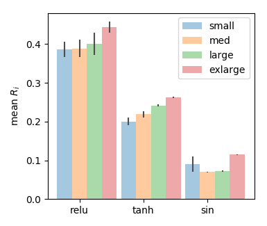
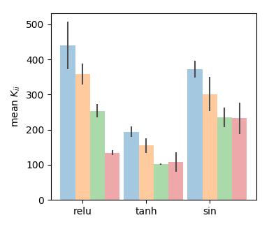
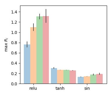
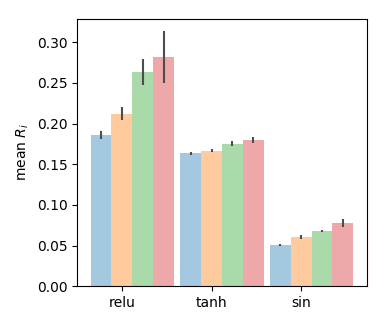
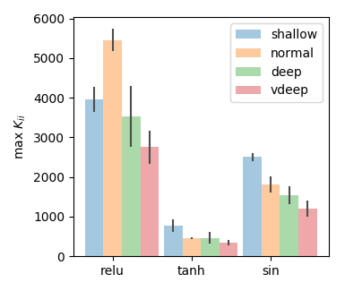
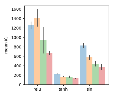
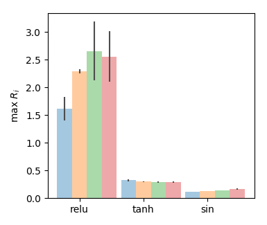
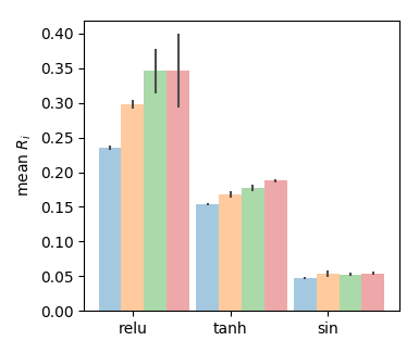
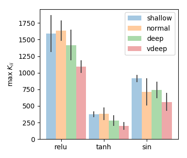
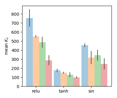
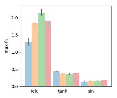
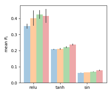
Based on Theorem 2, we are motivated to empirically evaluate two properties of the neural tangent kernel that appear relevant to stability in DQL: the magnitudes of diagonal elements, and the degree of off-diagonalness. To measure the latter, we consider the ratio of the average off-diagonal row entry to the on-diagonal entry, :
where is the size of the square matrix . We refer to this quantity as the ‘row ratio.’
We evaluate the standard neural networks used in DQL for continuous control: namely, feedforward multi-layer perceptrons with between 1 and 4 hidden layers, and between 32 and 256 hidden units, with either tanh, relu, or sin activations. (See, eg, (Lillicrap et al., 2016; Fujimoto et al., 2018b; Haarnoja et al., 2018b; Rajeswaran et al., 2017) for examples where networks in this range have previously been used.) Because divergence typically occurs near the beginning of training (van Hasselt et al., 2018) and the NTK is known to converge to a constant in the infinite-width limit (Jacot et al., 2018), we focus only on the properties of at initialization in these experiments.
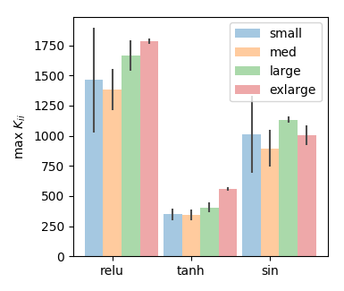
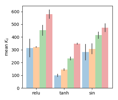
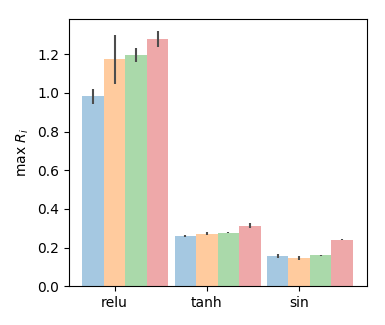
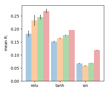
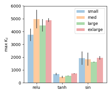
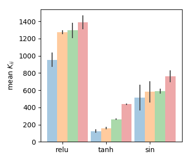
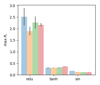
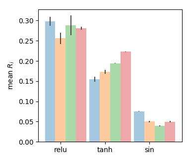
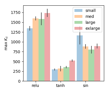
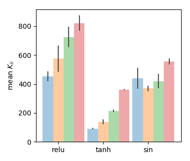
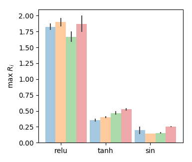
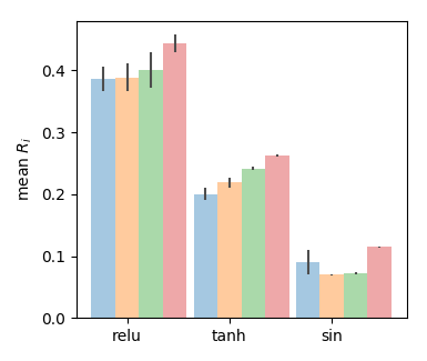
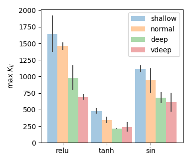
For each of three Gym environments (HalfCheetah-v2, Walker2d-v2, and Ant-v2), we sampled a dataset of 1000 state-action pairs using a “rails-random” policy: . We then randomly initialized neural networks of various sizes and activation functions, computed for each using the state-action pairs in , and evaluated their on-diagonal elements and average row ratios. We show partial results in Figure 1, complete results in Appendix C, and summarize findings here:
-
•
Diagonal elements tend to increase with width and decrease with depth, across activation functions.
-
•
Row ratios tend to increase with depth across activation functions, and do not clearly correlate with width.
-
•
Relu nets commonly have the largest on-diagonal elements and row ratios (so they should learn quickly and generalize aggressively).
-
•
Sin networks appear to be in a “sweet spot” of high on-diagonal elements and low off-diagonal elements. This analysis suggests sin activations may be more useful for DQL than has been previously realized.
Based on these results, as we will detail in subsequent sections, we experimented with using sin activations for TD3, SAC, and PreQN.
5.2 Benchmarking PreQN
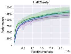
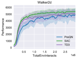
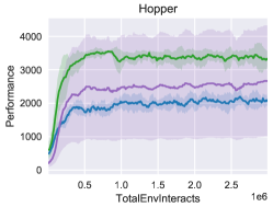
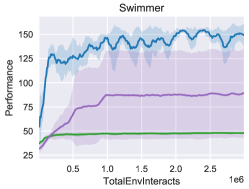
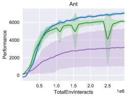
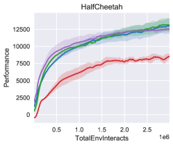
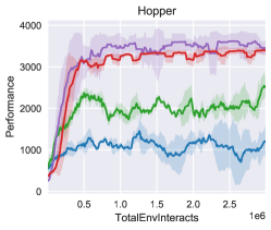
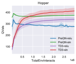
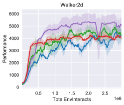
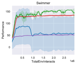
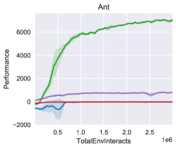
We benchmarked PreQN on five environments from the OpenAI Gym, comparing to TD3 and fixed-temperature SAC, and we present results in Figure 2. For each algorithm, we experimented with using relu and sin activations, and we found that PreQN performed best with sin activations, while TD3 and SAC performed best with relu activations. (As a result, we report results in our benchmark for PreQN-sin, TD3-relu, and SAC-relu.) However, we did not do any hyperparameter tuning for TD3 and SAC to specifically accomodate the sin activations, and instead relied on hyperparameters based on the literature which were well-tuned for relus. Hyperparameters for all experiments are given in Appendix B.
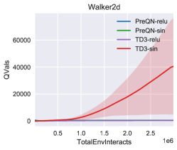
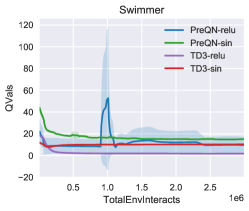
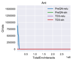
In general, PreQN is stable and performant, comparing favorably with the baseline algorithms. In some cases it outperforms (eg Swimmer and Ant) and in some cases it underperforms (eg Hopper). We find this outcome interesting and exciting because PreQN represents a different development path for DQL algorithms than is currently standard: it lacks target networks, only uses a single Q-function instead of multiple, makes no modifications to the bootstrap, and uses vanilla gradient steps for Q-learning instead of adaptive or momentum-based optimizers like Adam (Kingma & Ba, 2015). However (as we will shortly discuss), we found that it did not fully avert divergence when combined with relu networks.
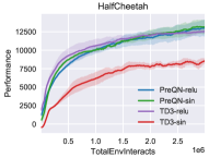
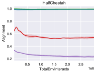
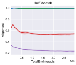
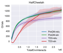
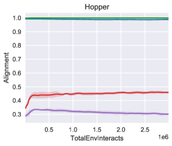
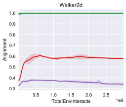
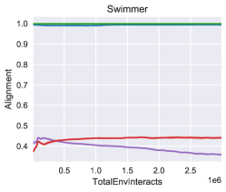
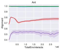
To measure how well DQL updates push -values towards their targets, we evaluated an alignment measure given by , where is the target for the algorithm ( in PreQN, and in TD3, where are the parameters of the slowly-changing target network). We show partial results in Figure 3 and complete results in Appendix D. We compared PreQN to TD3, because these two algorithms are equivalent except for the -learning component. While PreQN produces high alignment regardless of architecture by design, TD3 with the sin function (TD3-sin) produces updates that are better-aligned with their targets than TD3 with the relu function (TD3-relu). This accords well with our empirical analysis of the NTK: for sin networks, the NTK is closer to diagonal, so is closer to . Perhaps surprisingly, performance for TD3-sin was generally weaker than performance for TD3-relu, but we did not retune any of the hyperparameters from TD3-relu for TD3-sin; we speculate that better performance with TD3-sin may be achievable with a target network that updates more quickly. Performance for PreQN-relu was generally weaker than PreQN-sin, primarily due to occasional divergence; this result suggests that cancelling within-batch generalization is not a universal solution to divergence issues, and favorable architecture choices may be useful. However, in experiments not included in this report, we found that divergence issues with PreQN-relu were straightforwardly resolved by decreasing the learning rate (at a nontrivial cost to performance).
We are intrigued by the fact that empirical analysis of the NTK successfully predicts how the cosine alignment of a DQL update changes with architecture in the TD3 experiments. It has been observed that architecture changes can have a significant effect on performance in deep RL (for example, see Henderson et al. (2018)), but to the best of our knowledge, no one has previously proposed any method for predicting how the behavior of a given algorithm might change with architecture. Based on our results, we are cautiously optimistic that the NTK is the correct object of study for such predictions, and we recommend a more rigorous empirical analysis relating NTK measurements, architectures, and hyperparameter choices in DQL to performance.
5.3 Remarks on Computational Cost
Our implementation of PreQN was significantly slower than our implementation of SAC (by more than 50%), due to the requirement of calculating backward passes separately for each state-action pair in the batch, and solving the system of equations . However, we consider it plausible that many adjustments could be made to reduce computational cost from our basic code. (For instance: we did not reuse the gradients from computing for forming the update, , and this redundancy can be eliminated.)
6 Other Related Work
Previously, Melo et al. (2008) proved sufficient conditions for the convergence of -learning with linear function approximators. Their conditions were fairly restrictive, essentially requiring that the algorithm behave as if it were on-policy—removing one of the components of the triad. We see an interesting parallel to our results for the linear approximation case (Theorem 2), which also effectively remove a component of the triad by requiring the algorithm to behave as if it were tabular.
Concurrently to our work, (Bhatt et al., 2019) developed CrossNorm, a variant of DDPG that uses a careful application of BatchNorm (Ioffe & Szegedy, 2015) to achieve stable learning without target networks. Also concurrently, Fu et al. (2019) performed a rigorous empirical study of Fitted Q-Iteration (FQI) (Riedmiller, 2005) to gain insight into divergence issues in DQL, and ultimately proposed an algorithm based on data distribution modifications to improve performance.
7 Conclusions
In this work, we examined how -values change under a DQL update in order to understand how divergence might arise. We used our insights to develop a practical algorithm, called PreQN, which attacks one of the root causes of divergence: the generalization properties of the -function approximator, as quantified by the neural tangent kernel (Jacot et al., 2018). Our experiments show that PreQN, with appropriate design choices, is stable and performant on various high-dimensional continuous control tasks.
Intriguingly, theoretical and empirical work shows that the NTK converges to a constant (independent of network parameters) in the limit of wide networks (Jacot et al., 2018); this result makes it possible to study the evolution of neural network functions through their linearization around the starting point (Lee et al., 2019). In this regime, through the correspondence in Lemma 3, DQL should behave quite closely to linear TD-learning. We consider the detailed analysis of this connection to be an interesting avenue for potential future work.
References
- Amari (1998) Amari, S. I. Natural Gradient Works Efficiently in Learning. Neural Computation, 10(2):251–276, 1998. ISSN 08997667. doi: 10.1162/089976698300017746.
- Baird (1995) Baird, L. C. Residual Algorithms: Reinforcement Learning with Function Approximation. Proceedings of the Machine Learning Conference, pp. 30–37, 1995. ISSN 1098-6596. doi: 10.1017/CBO9781107415324.004. URL http://leemon.com/papers/1995b.pdf.
- Bhatt et al. (2019) Bhatt, A., Argus, M., Amiranashvili, A., and Brox, T. CrossNorm: Normalization for Off-Policy TD Reinforcement Learning. feb 2019. URL http://arxiv.org/abs/1902.05605.
- Brockman et al. (2016) Brockman, G., Cheung, V., Pettersson, L., Schneider, J., Schulman, J., Tang, J., and Zaremba, W. OpenAI Gym. 2016. URL http://arxiv.org/abs/1606.01540.
- Durugkar & Stone (2017) Durugkar, I. and Stone, P. TD Learning With Constrained Gradients. Deep Reinforcement Learning Symposium, NIPS 2017, 2017. URL https://openreview.net/pdf?id=Bk-ofQZRb.
- Fox et al. (2016) Fox, R., Pakman, A., and Tishby, N. Taming the Noise in Reinforcement Learning via Soft Updates. In Uncertainty in Artificial Intelligence, 2016. URL http://arxiv.org/abs/1512.08562.
- Fu et al. (2019) Fu, J., Kumar, A., Soh, M., and Levine, S. Diagnosing Bottlenecks in Deep Q-learning Algorithms. Technical report, 2019. URL http://arxiv.org/abs/1902.10250.
- Fujimoto et al. (2018a) Fujimoto, S., Meger, D., and Precup, D. Off-Policy Deep Reinforcement Learning without Exploration. Technical report, dec 2018a. URL http://arxiv.org/abs/1812.02900.
- Fujimoto et al. (2018b) Fujimoto, S., van Hoof, H., and Meger, D. Addressing Function Approximation Error in Actor-Critic Methods. In International Conference on Machine Learning, feb 2018b. URL http://arxiv.org/abs/1802.09477.
- Gauci et al. (2018) Gauci, J., Conti, E., Liang, Y., Virochsiri, K., He, Y., Kaden, Z., Narayanan, V., and Ye, X. Horizon: Facebook’s Open Source Applied Reinforcement Learning Platform. Technical report, 2018. URL http://arxiv.org/abs/1811.00260.
- Gordon (1995) Gordon, G. J. Stable Function Approximation in Dynamic Programming. In Proceedings of the International Conference on Machine Learning, 1995. ISBN 9781558603776. doi: 10.1016/B978-1-55860-377-6.50040-2. URL https://www.sciencedirect.com/science/article/pii/B9781558603776500402.
- Haarnoja et al. (2018a) Haarnoja, T., Zhou, A., Ha, S., Tan, J., Tucker, G., and Levine, S. Learning to Walk via Deep Reinforcement Learning. Technical report, dec 2018a. URL http://arxiv.org/abs/1812.11103.
- Haarnoja et al. (2018b) Haarnoja, T., Zhou, A., Hartikainen, K., Tucker, G., Ha, S., Tan, J., Kumar, V., Zhu, H., Gupta, A., Abbeel, P., and Levine, S. Soft Actor-Critic Algorithms and Applications. Technical report, dec 2018b. URL http://arxiv.org/abs/1812.05905.
- Henderson et al. (2018) Henderson, P., Islam, R., Bachman, P., Pineau, J., Precup, D., and Meger, D. Deep Reinforcement Learning that Matters. In Thirty-Second AAAI Conference On Artificial Intelligence (AAAI), 2018. URL http://arxiv.org/abs/1709.06560.
- Hessel et al. (2017) Hessel, M., Modayil, J., van Hasselt, H., Schaul, T., Ostrovski, G., Dabney, W., Horgan, D., Piot, B., Azar, M., and Silver, D. Rainbow: Combining Improvements in Deep Reinforcement Learning. oct 2017. URL http://arxiv.org/abs/1710.02298.
- Horgan et al. (2018) Horgan, D., Quan, J., Budden, D., Barth-Maron, G., Hessel, M., van Hasselt, H., and Silver, D. Distributed Prioritized Experience Replay. In International Conference on Learning Representations, 2018. URL http://arxiv.org/abs/1803.00933.
- Ioffe & Szegedy (2015) Ioffe, S. and Szegedy, C. Batch Normalization: Accelerating Deep Network Training by Reducing Internal Covariate Shift. Technical report, 2015. URL http://arxiv.org/abs/1502.03167.
- Jacot et al. (2018) Jacot, A., Gabriel, F., and Hongler, C. Neural Tangent Kernel: Convergence and Generalization in Neural Networks. Technical report, jun 2018. URL http://arxiv.org/abs/1806.07572.
- Kalashnikov et al. (2018) Kalashnikov, D., Irpan, A., Pastor, P., Ibarz, J., Herzog, A., Jang, E., Quillen, D., Holly, E., Kalakrishnan, M., Vanhoucke, V., and Levine, S. QT-Opt: Scalable Deep Reinforcement Learning for Vision-Based Robotic Manipulation. In Conference on Robot Learning, 2018. URL http://arxiv.org/abs/1806.10293.
- Kapturowski et al. (2019) Kapturowski, S., Ostrovski, G., Quan, J., Munos, R., and Dabney, W. Recurrent Experience Replay in Distributed Reinforcement Learning. International Conference on Learning Representation, 2019.
- Kingma & Ba (2015) Kingma, D. P. and Ba, J. Adam: A Method for Stochastic Optimization. In International Conference for Learning Representations, 2015. URL http://arxiv.org/abs/1412.6980.
- Knight & Lerner (2018) Knight, E. and Lerner, O. Natural Gradient Deep Q-learning. Technical report, 2018. URL https://arxiv.org/pdf/1803.07482.pdf.
- Lee et al. (2019) Lee, J., Xiao, L., Schoenholz, S. S., Bahri, Y., Sohl-Dickstein, J., and Pennington, J. Wide Neural Networks of Any Depth Evolve as Linear Models Under Gradient Descent. Technical report, 2019. URL https://arxiv.org/abs/1902.06720.
- Lillicrap et al. (2016) Lillicrap, T. P., Hunt, J. J., Pritzel, A., Heess, N., Erez, T., Tassa, Y., Silver, D., and Wierstra, D. Continuous control with deep reinforcement learning. In International Conference on Learning Representations, 2016. URL http://arxiv.org/abs/1509.02971.
- Lin (1992) Lin, L.-J. Self-Improving Reactive Agents Based On Reinforcement Learning, Planning and Teaching. Machine Learning, 8:293–321, 1992. URL http://www.incompleteideas.net/lin-92.pdf.
- Melo et al. (2008) Melo, F. S., Meyn, S. P., and Ribeiro, M. I. An Analysis of Reinforcement Learning with Function Approximation. In International Conference on Machine Learning, 2008. URL http://icml2008.cs.helsinki.fi/papers/652.pdf.
- Mnih et al. (2013) Mnih, V., Silver, D., and Riedmiller, M. Playing Atari with Deep Q Learning. Technical report, 2013.
- Mnih et al. (2015) Mnih, V., Kavukcuoglu, K., Silver, D., Rusu, A. A., Veness, J., Bellemare, M. G., Graves, A., Riedmiller, M., Fidjeland, A. K., Ostrovski, G., Petersen, S., Beattie, C., Sadik, A., Antonoglou, I., King, H., Kumaran, D., Wierstra, D., Legg, S., and Hassabis, D. Human-level control through deep reinforcement learning. Nature, 518(7540):529–533, feb 2015. ISSN 0028-0836. doi: 10.1038/nature14236. URL http://www.nature.com/articles/nature14236.
- Nair et al. (2015) Nair, A., Srinivasan, P., Blackwell, S., Alcicek, C., Fearon, R., De Maria, A., Panneershelvam, V., Suleyman, M., Beattie, C., Petersen, S., Legg, S., Mnih, V., Kavukcuoglu, K., and Silver, D. Massively Parallel Methods for Deep Reinforcement Learning. Technical report, 2015. URL http://arxiv.org/abs/1507.04296.
- Pohlen et al. (2018) Pohlen, T., Piot, B., Hester, T., Azar, M. G., Horgan, D., Budden, D., Barth-Maron, G., van Hasselt, H., Quan, J., Večerík, M., Hessel, M., Munos, R., and Pietquin, O. Observe and Look Further: Achieving Consistent Performance on Atari. Technical report, 2018. URL http://arxiv.org/abs/1805.11593.
- Rajeswaran et al. (2017) Rajeswaran, A., Lowrey, K., Todorov, E., and Kakade, S. Towards Generalization and Simplicity in Continuous Control. In Neural Information Processing Systems, 2017. URL http://arxiv.org/abs/1703.02660.
- Riedmiller (2005) Riedmiller, M. Neural Fitted Q Iteration. Lecture Notes in Computer Science (including subseries Lecture Notes in Artificial Intelligence and Lecture Notes in Bioinformatics), 3720 LNAI:317–328, 2005. ISSN 03029743. doi: 10.1007/11564096˙32.
- Schulman et al. (2017) Schulman, J., Chen, X., and Abbeel, P. Equivalence Between Policy Gradients and Soft Q-Learning. 2017. URL http://arxiv.org/abs/1704.06440.
- Sidor & Schulman (2017) Sidor, S. and Schulman, J. OpenAI Baselines: DQN, 2017. URL https://blog.openai.com/openai-baselines-dqn/.
- Sutton & Barto (2018) Sutton, R. and Barto, A. G. Reinforcement Learning: An Introduction. MIT Press, 2018. URL http://incompleteideas.net/book/the-book.html.
- Sutton (1988) Sutton, R. S. Learning to predict by the methods of temporal differences. Machine Learning, 3(1):9–44, aug 1988. ISSN 0885-6125. doi: 10.1007/BF00115009. URL http://link.springer.com/10.1007/BF00115009.
- Tsitsiklis & Roy (1997) Tsitsiklis, J. N. and Roy, B. V. An Analysis of Temporal-Difference Learning with Function Approximation. Technical Report 5, 1997. URL http://www.mit.edu/{~}jnt/Papers/J063-97-bvr-td.pdf.
- van Hasselt et al. (2016) van Hasselt, H., Guez, A., and Silver, D. Deep Reinforcement Learning with Double Q-learning. In AAAI, 2016. URL http://arxiv.org/abs/1509.06461.
- van Hasselt et al. (2018) van Hasselt, H., Doron, Y., Strub, F., Hessel, M., Sonnerat, N., and Modayil, J. Deep Reinforcement Learning and the Deadly Triad. Technical report, dec 2018. URL http://arxiv.org/abs/1812.02648.
- Wang et al. (2016) Wang, Z., Schaul, T., Hessel, M., van Hasselt, H., Lanctot, M., and de Freitas, N. Dueling Network Architectures for Deep Reinforcement Learning. In International Conference on Machine Learning, 2016. URL http://arxiv.org/abs/1511.06581.
- Watkins & Dayan (1992) Watkins, C. J. C. H. and Dayan, P. Q-learning. Machine Learning, 8(3-4):279–292, 1992. ISSN 0885-6125. doi: 10.1007/BF00992698. URL http://link.springer.com/10.1007/BF00992698.
- Yang et al. (2019) Yang, Z., Xie, Y., and Wang, Z. A Theoretical Analysis of Deep Q-Learning. Technical report, jan 2019. URL http://arxiv.org/abs/1901.00137.
Appendix A Proofs
See 1
Proof.
To establish that is a contraction, we compute:
Thus contracts with modulus . That is the fixed-point follows immediately from .
∎
See 2
Proof.
First, we observe that for any , we have:
Then, by taking the max over on both sides (first the right, and then the left), we obtain:
where . If (which is equivalent to the condition ), then the modulus and is a contraction. That its fixed-point is follows from .
However, if , we merely have an upper bound on and that alone is not sufficient to demonstate that is a not a contraction. This is easy to demonstrate without resorting to inequalities, though: for any with , it is straightforward to see that —that is, leaves that -value unchanged. Thus there are choices of such that and is a non-expansion. ∎
See 3
Proof.
For the linear function approximation case, , and the NTK (Eq. 9) therefore has components
which are independent of . Thus .
Furthermore, for all and all , so all higher-order terms are zero. ∎
See 2
Proof.
Using index notation instead of tracking state-action pairs,
Thus we can obtain a modulus as . We’ll break it up into on-diagonal and off-diagonal parts, and assume that :
A guarantee that can then be obtained by requiring that
We note that this is a quite restrictive condition, since for high, will be quite large, and the LHS has a sum over all off-diagonal terms in a row.
∎
See 3
Proof.
First, to obtain Eq. 18:
| Iterate sequence and fixed-point assumption | ||||
| Definition of Lipschitz continuity | ||||
| Repeated application of above |
That the sequence converges to follows from
when . ∎
See 4
Proof.
Let have rank and a singular value decomposition given by , with . Recall that . Then and , and:
∎
Appendix B Methods for PreQN Benchmark
We used the following hyperparameters for our PreQN benchmark experiments:
| Hyperparameter | Value | |
|---|---|---|
| Discount factor | ||
| Batch size | ||
| Network size | ||
| Actor learning rate | ||
| Actor optimizer | Adam | |
| Critic learning rate | for TD3 and SAC, | for PreQN |
| Update frequency | ||
| Update after | ||
| Start steps | ||
| Alignment threshold (PreQN only) | ||
| Action noise (TD3 and PreQN) | ||
| Target network polyak averaging (TD3 and SAC) | ||
| Entropy regularization coefficient (SAC only) |
Here, ‘update frequency’ refers to the number of environment steps that would elapse between occasions of updating the networks. During each update, there would be as many gradient descent steps (and target network polyak-averaging steps, if applicable) as environment steps had elapsed since the last update (so that for the overall training run, the ratio of gradient steps to env steps would be 1:1).
‘Update after’ refers to the number of steps that would elapse at the beginning of training before any gradient descent steps would take place (to allow time for filling the replay buffer).
For improved exploration, at the beginning of training agents would spend ‘start steps’ number of steps acting under a uniform random policy.
TD3 hyperparameters for target policy smoothing and policy delay were taken from (Fujimoto et al., 2018b) without modification.
Appendix C Extended Results for Neural Tangent Kernel Analysis
C.1 Experiments with Network Width
C.2 Experiments with Network Depth
Appendix D Extended Results for Alignment Experiment with Architecture Ablation
