Fair sampling of ground-state configurations of binary optimization problems
Abstract
Although many efficient heuristics have been developed to solve binary optimization problems, these typically produce correlated solutions for degenerate problems. Most notably, transverse-field quantum annealing—the heuristic employed in current commercially available quantum annealing machines—has been shown to often be exponentially biased when sampling the solution space. Here we present an approach to sample ground-state (or low-energy) configurations for binary optimization problems. The method samples degenerate states with almost equal probability and is based on a combination of parallel tempering Monte Carlo with isoenergetic cluster moves. We illustrate the approach using two-dimensional Ising spin glasses, as well as spin glasses on the D-Wave Systems quantum annealer chimera topology. In addition, a simple heuristic to approximate the number of solutions of a degenerate problem is introduced.
pacs:
75.50.Lk, 75.40.Mg, 05.50.+q, 64.60.-iI Introduction
Quantum annealing Finnila et al. (1994); Kadowaki and Nishimori (1998); Brooke et al. (1999); Farhi et al. (2001); Santoro et al. (2002); Das and Chakrabarti (2005); Santoro and Tosatti (2006); Das and Chakrabarti (2008); Morita and Nishimori (2008) and, in particular, quantum annealing machines have ignited an ever-increasing interest in algorithms used in statistical physics to solve hard combinatorial industrial optimization problems, as well as related applications. While there has been an extensive body of work attempting to discern if the D-Wave Systems special-purpose quantum annealing machine can outperform algorithms on conventional CMOS hardware Dickson et al. (2013); Pudenz et al. (2014); Smith and Smolin (2013); Boixo et al. (2013); Albash et al. (2015a); Rønnow et al. (2014); Katzgraber et al. (2014); Lanting et al. (2014); Santra et al. (2014); Shin et al. (2014); Boixo et al. (2014); Albash et al. (2015b, a); Katzgraber et al. (2015); Martin-Mayor and Hen (2015); Pudenz et al. (2015); Hen et al. (2015); Venturelli et al. (2015); Vinci et al. (2015); Zhu et al. (2016); Mandrà et al. (2016); Mandrà and Katzgraber (2017); Mandrá and Katzgraber (2018), there have been only a few studies Boixo et al. (2013); Albash et al. (2014); King et al. (2016); Mandrà et al. (2017); Könz et al. (2018) attempting to characterize the sampling ability of quantum annealing. Initial studies Matsuda et al. (2009); Mandrà et al. (2017) suggested that transverse-field quantum annealing with stoquastic drivers result in biased solution distributions for degenerate problems. However, more recently, it was shown Könz et al. (2018) that even with high-order drivers the sampling bias can be removed only in special cases.
Many industrial applications rely more on a broad solution pool then on the minimum of the cost function, with some prominent examples being propositional model counting and related problems Jerrum et al. (1986); Gomes et al. (2008); Gopalan et al. (2011), SAT-based probabilistic membership filters Weaver et al. (2014); Schaefer (1978); Douglass et al. (2015); Herr et al. (2017), machine learning applications Hinton (2002); Eslami et al. (2014), or simply estimating the ground-state entropy of a degenerate system. In addition, having multiple solutions to a given problem might allow for the inclusion of constraints in a post-processing step. Here we demonstrate that Monte Carlo methods paired with cluster updates can result in algorithms that asymptotically sample ground-states fairly.
Classical Monte Carlo heuristics based on thermal annealing are known to almost uniformly sample all ground-state and low-lying excited state configurations Moreno et al. (2003); Wang et al. (2015). Studies of three-dimensional diluted Ising antiferromagnets in a field and three-dimensional Ising spin glasses show that parallel tempering Monte Carlo Hukushima and Nemoto (1996) is more efficient than simulated annealing Kirkpatrick et al. (1983) at finding spin-glass ground-state configurations with near-equal probability Moreno et al. (2003); com (a). Isoenergetic cluster moves (ICM) Zhu et al. (2015), related to Houdayer’s cluster updates Houdayer (2001), introduced for Ising spin glasses significantly speed up thermalization on quasi-two-dimensional topologies, such as D-Wave’s Chimera graph. The combination of low-temperature parallel tempering (PT) Monte Carlo and the rejection-free isoenergetic cluster moves (PT+ICM) allow for a wide-spread sampling of search space and help escape local minima separated by large energy barriers. Here we demonstrate that isoenergetic cluster moves paired with parallel tempering Monte Carlo (PT+ICM) enhance the fair sampling of ground-state configurations for spin-glass problems better than the previous PT gold standard. We illustrate the approach using two-dimensional Ising spin glasses on a square lattice, as well as the Chimera graph. Higher-dimensional problems can be embedded in lower-dimensional graphs where PT+ICM is more efficient via, e.g., minor embedding Choi (2008, 2011).
The paper is organized as follows. In Sec. II we introduce a quality metric for fair sampling, as well as a detailed description of a fair-sampling algorithm using ICM. Following that, we present numerical results in Sec. III for both PT, as well as PT+ICM, and introduce an algorithm to approximate the number of degenerate states for highly-degenerate problems. We conclude with a discussion of our results.
II Model and Algorithm
To illustrate the improved sampling of PT+ICM over PT, we start with an Ising spin-glass model on a nonplanar Chimera graph Bunyk et al. (2014). Its nonplanar topology makes finding ground states of random Ising spin glasses worst-case NP-hard. The Hamiltonian for the spin-glass model is given by
| (1) |
where are Ising spins and the couplers are drawn for this study from three discrete distributions: , and ). The couplers are selected based on the range of ground-state degeneracy we can handle with our high-performance computing cluster; i.e., the less symmetries between the different coupler values, the smaller the ground-state degeneracy.
II.1 Assessing optimal sampling
Suppose is the total number of times that ground states are found for an instance with ground-state degeneracy . The probability distribution for finding any particular ground-state configuration follows a binomial distribution. For theoretically perfect sampling, if is the probability of finding a state and is the probability of failure in a given trial, then the expected number of successes in trials is and the variance of the binomial distribution is . Therefore, the theoretical relative standard deviation given by sampling a finite set of random uncorrelated numbers is given by
| (2) |
Assuming that the states are uncorrelated (which is a safe assumption for large ), an algorithm is said to be optimal (sampling fairly) if the numerical relative standard deviation of the frequency of ground-state configurations determined experimentally is close or equal to the theoretical value (or ). In practice, for any algorithm is almost always greater than the theoretical value , due to a limited number of measurements via e.g., limited computing resources.
II.2 PT+ICM for fair sampling
Our implementation of PT+ICM for sampling purposes can be summarized as follows:
-
1.
Run replicas of the system at a range of temperatures {}, with each set consisting of copies of the system at the same temperature, thus copies of the system with the same disorder are randomly initialized.
-
2.
iterations are performed, each iteration consisting of one Monte Carlo sweep, a parallel tempering update, and an isoenergetic cluster move (for the lowest temperatures).
-
3.
For the first iterations, keep track of the lowest energies for the four replicas at the lowest temperatures.
-
4.
After iterations, the lowest energies , , , and for the four replicas with the lowest temperatures are compared, and if , the ground-state energy has been found with high confidence. Once this is the case, configurations at this energy are recorded, as well as their frequency for the remaining /2 updates.
There is no guarantee that any solution obtained by this heuristic method is the true optimum, or that we have found all configurations that minimize the Hamiltonian. However, we choose to make sure each configuration achieves a minimum number of hits in order to increase our confidence that all accessible ground states have been found. The simulation parameters are shown in Table 1.
| Topology | Couplers | |||||||
| 2D | ||||||||
| 2D | ||||||||
| 2D | ||||||||
| 2D | ||||||||
| 2D | ||||||||
| Chimera | ||||||||
| Chimera | ||||||||
| Chimera | ||||||||
| Chimera | ||||||||
| Chimera | ||||||||
| Chimera |
III Numerical results
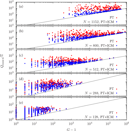
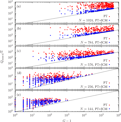
To test whether PT+ICM can sample ground-state configurations with near-equal probabilities, we multiply the numerical relative standard deviation by and plot as a function of the ground-state degeneracy . Note that is the square root of the ground-state degeneracy , and therefore the function is a straight line in logarithmic scale for both the horizontal axis () and the vertical axis ().
Figure 1 shows and as a function of the ground-state degeneracy for different spin-glass instances on a Chimera graph. As mentioned in the previous paragraph, the quantity is almost always greater than due to limited computational resources com (b). However, an algorithm samples optimally if the data from the numerical relative standard deviation are close to the theoretical line. It is clear that the data for PT+ICM (blue/darker color) are closer to a straight line than the data for PT (red/lighter color), and the discrepancy between PT+ICM and PT seems to become greater as the system size increases.
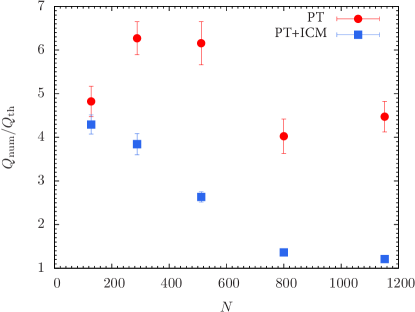
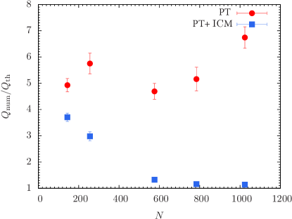
In Fig. 2 we plot the median ratio as a function of the system size for spin-glass problems on a Chimera lattice. We emphasize that when the ratio becomes unity an algorithm samples optimally. The data show that PT+ICM (blue squares) performs better than PT (red circles) and that the improvement is more significant with increasing system size. In this work the temperature set for the simulation is specifically optimized for . Large median ratios for smaller system sizes are due to the choice of temperature set. The statistical error bars are determined by a bootstrap analysis using the following procedure: For each system size and disorder realizations, a randomly selected bootstrap sample of the disorder realizations is generated. The median ratio is computed with this random sample. We repeat this procedure times for each system size to obtain an average and error bar using these data points.
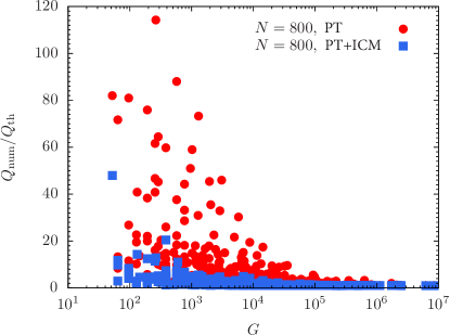
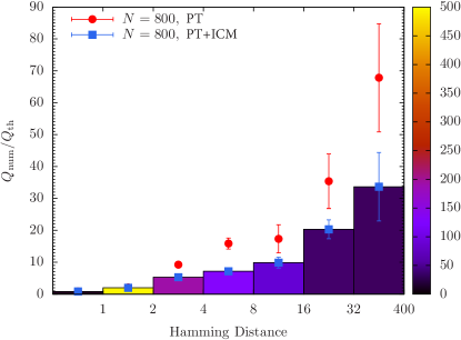
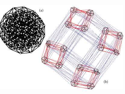
In addition to studying how fair sampling behaves with increasing system size, we also investigate how the quality of fair sampling is related to ground-state degeneracy and plot as a function of ground-state degeneracy for variables. Figure 3 suggests that the more ground-state configurations, the easier to sample all ground-state configurations with near-equal probabilities. This is not surprising because a large ground-state manifold makes the algorithm easier to explore the configuration space. We do emphasize, however, that in cases where the ground-state degeneracy is exponentially large and with limited resources only a subset of minimizing configurations is accessible, and for these the sampling improves, the more configurations are present. Furthermore, careful examination of instances with the same system size and ground-state degeneracy suggests that the ratio is closely related to the Hamming distances between ground-state configurations. It is shown in Fig. 4 that the Sidon instances Katzgraber et al. (2015); Zhu et al. (2016) where with large Hamming distances between the ground-state configurations tend to have a high ratio compared to those with small Hamming distances between the states. Here, PT+ICM achieves more equiprobable sampling with large Hamming distances. Figure 5 shows two examples of ground-state configurations with different Hamming distances on a Chimera graph with . PT+ICM’s cluster updates allow nonlocal moves in the energy landscape, therefore reducing for instances with large Hamming distances between the ground-state configurations.
Figure 6 shows and as a function of the ground-state degeneracy for different spin-glass instances on a two-dimensional square lattice. Similar to the Chimera graph case, the data using PT+ICM (blue/dark color) are closer to the theoretical optimality line than the data using PT (red/light color), and the discrepancy between PT+ICM and PT becomes larger as the system size increases. In Fig. 7, the median ratio again demonstrates that PT+ICM is superior to PT in this case for square lattices.
III.1 Estimating the ground-state degeneracy
We also develop an approximate method to count the number of ground-state configurations based on the fair sampling capabilities of PT+ICM and compare the results to exact methods Galluccio et al. (2000) for a handful of configurations. Counting problems Gomes et al. (2008) typically ask how many solutions exist for a given instance and belong to complexity class of #P. This approximate method exploits the fact that if one can sample ground states uniformly then one can obtain a reasonable order-of-magnitude estimate of the ground-state degeneracy. Our renormalization-inspired approach works as follows:
-
1.
Compute the ground-state energy for a fixed number of Monte Carlo sweeps (see above).
-
2.
Sample the number of ground states for the full system for a fixed number of Monte Carlo sweeps.
-
3.
Iteratively restrict the number of free variables (i.e., those that are not restricted) and estimate the ratio
for a fixed number of Monte Carlo sweeps.
-
4.
Repeat until the system size is small enough to be able to compute the number of ground state configurations exactly, e.g., via enumeration.
-
5.
Multiply the product of ratios by the exact count of ground-state configurations to estimate the number of ground states for the full system via
We compare results of this approximate method to exact counts on a two-dimensional square lattice with bimodal coupling constants . Simulation parameters and results are shown in Table 2. The renormalization-based estimates agree with the exact ground-state degeneracy within error bars.
| Instance | error | % error | ||
|---|---|---|---|---|
IV Conclusions
We have demonstrated that PT+ICM—parallel tempering Monte Carlo with isoenergetic cluster moves—samples ground-state configurations fairly and is an ideal method for applications where a pool of diverse solutions is needed. We also find that degeneracy and Hamming distances between different ground-state configurations are closely related to the relative standard deviation of frequency with which the ground states are found, namely: ground states with large degeneracy and small Hamming distances have a lower relative standard deviation of frequency. It will be interesting to exploit near-uniform sampling for model counting Wei and Selman (2005) and SAT filter construction Weaver et al. (2014); Douglass et al. (2015) in the future.
Acknowledgements.
We would like to thank Ruben S. Andrist, Hamid Khoshbakht, Martin Weigel and Salvatore Mandrà for fruitful discussions. We especially thank Martin Weigel for providing the exact number of ground-state configurations on two-dimensional square lattices using the Vondrak code, and Ruben S. Andrist for rendering Fig. 5. H.G.K. acknowledges support from the National Science Foundation (Grant No. DMR-1151387) and would like to thank Banh Mi for providing the necessary motivation for this research. We thank the Texas Advanced Computing Center (TACC) at The University of Texas at Austin and Texas A&M University for providing HPC resources. Part of this research is based upon work supported in part by the Office of the Director of National Intelligence (ODNI), Intelligence Advanced Research Projects Activity (IARPA), via MIT Lincoln Laboratory Air Force Contract No. FA8721-05-C-0002. The views and conclusions contained herein are those of the authors and should not be interpreted as necessarily representing the official policies or endorsements, either expressed or implied, of ODNI, IARPA, or the U.S. Government. The U.S. Government is authorized to reproduce and distribute reprints for Governmental purposes notwithstanding any copyright annotation thereon.References
- Finnila et al. (1994) A. B. Finnila, M. A. Gomez, C. Sebenik, C. Stenson, and J. D. Doll, Chem. Phys. Lett. 219, 343 (1994).
- Kadowaki and Nishimori (1998) T. Kadowaki and H. Nishimori, Phys. Rev. E 58, 5355 (1998).
- Brooke et al. (1999) J. Brooke, D. Bitko, T. F. Rosenbaum, and G. Aepli, Science 284, 779 (1999).
- Farhi et al. (2001) E. Farhi, J. Goldstone, S. Gutmann, J. Lapan, A. Lundgren, and D. Preda, Science 292, 472 (2001).
- Santoro et al. (2002) G. Santoro, E. Martoňák, R. Tosatti, and R. Car, Science 295, 2427 (2002).
- Das and Chakrabarti (2005) A. Das and B. K. Chakrabarti, Quantum Annealing and Related Optimization Methods (Edited by A. Das and B.K. Chakrabarti, Lecture Notes in Physics 679, Berlin: Springer, 2005).
- Santoro and Tosatti (2006) G. E. Santoro and E. Tosatti, J. Phys. A 39, R393 (2006).
- Das and Chakrabarti (2008) A. Das and B. K. Chakrabarti, Rev. Mod. Phys. 80, 1061 (2008).
- Morita and Nishimori (2008) S. Morita and H. Nishimori, J. Math. Phys. 49, 125210 (2008).
- Dickson et al. (2013) N. G. Dickson, M. W. Johnson, M. H. Amin, R. Harris, F. Altomare, A. J. Berkley, P. Bunyk, J. Cai, E. M. Chapple, P. Chavez, et al., Nat. Commun. 4, 1903 (2013).
- Pudenz et al. (2014) K. L. Pudenz, T. Albash, and D. A. Lidar, Nat. Commun. 5, 3243 (2014).
- Smith and Smolin (2013) G. Smith and J. A. Smolin, Physics 6, 105 (2013).
- Boixo et al. (2013) S. Boixo, T. Albash, F. M. Spedalieri, N. Chancellor, and D. A. Lidar, Nat. Commun. 4, 2067 (2013).
- Albash et al. (2015a) T. Albash, T. F. Rønnow, M. Troyer, and D. A. Lidar, Eur. Phys. J. Spec. Top. 224, 111 (2015a).
- Rønnow et al. (2014) T. F. Rønnow, Z. Wang, J. Job, S. Boixo, S. V. Isakov, D. Wecker, J. M. Martinis, D. A. Lidar, and M. Troyer, Science 345, 420 (2014).
- Katzgraber et al. (2014) H. G. Katzgraber, F. Hamze, and R. S. Andrist, Phys. Rev. X 4, 021008 (2014).
- Lanting et al. (2014) T. Lanting, A. J. Przybysz, A. Y. Smirnov, F. M. Spedalieri, M. H. Amin, A. J. Berkley, R. Harris, F. Altomare, S. Boixo, P. Bunyk, et al., Phys. Rev. X 4, 021041 (2014).
- Santra et al. (2014) S. Santra, G. Quiroz, G. Ver Steeg, and D. A. Lidar, New J. Phys. 16, 045006 (2014).
- Shin et al. (2014) S. W. Shin, G. Smith, J. A. Smolin, and U. Vazirani (2014), (arXiv:1401.7087).
- Boixo et al. (2014) S. Boixo, T. F. Rønnow, S. V. Isakov, Z. Wang, D. Wecker, D. A. Lidar, J. M. Martinis, and M. Troyer, Nat. Phys. 10, 218 (2014).
- Albash et al. (2015b) T. Albash, W. Vinci, A. Mishra, P. A. Warburton, and D. A. Lidar, Phys. Rev. A 91, 042314 (2015b).
- Katzgraber et al. (2015) H. G. Katzgraber, F. Hamze, Z. Zhu, A. J. Ochoa, and H. Munoz-Bauza, Phys. Rev. X 5, 031026 (2015).
- Martin-Mayor and Hen (2015) V. Martin-Mayor and I. Hen, Nature Scientific Reports 5, 15324 (2015).
- Pudenz et al. (2015) K. L. Pudenz, T. Albash, and D. A. Lidar, Phys. Rev. A 91, 042302 (2015).
- Hen et al. (2015) I. Hen, J. Job, T. Albash, T. F. Rønnow, M. Troyer, and D. A. Lidar, Phys. Rev. A 92, 042325 (2015).
- Venturelli et al. (2015) D. Venturelli, S. Mandrà, S. Knysh, B. O’Gorman, R. Biswas, and V. Smelyanskiy, Phys. Rev. X 5, 031040 (2015).
- Vinci et al. (2015) W. Vinci, T. Albash, G. Paz-Silva, I. Hen, and D. A. Lidar, Phys. Rev. A 92, 042310 (2015).
- Zhu et al. (2016) Z. Zhu, A. J. Ochoa, F. Hamze, S. Schnabel, and H. G. Katzgraber, Phys. Rev. A 93, 012317 (2016).
- Mandrà et al. (2016) S. Mandrà, Z. Zhu, W. Wang, A. Perdomo-Ortiz, and H. G. Katzgraber, Phys. Rev. A 94, 022337 (2016).
- Mandrà and Katzgraber (2017) S. Mandrà and H. G. Katzgraber, Quantum Sci. Technol. 2, 038501 (2017).
- Mandrá and Katzgraber (2018) S. Mandrá and H. G. Katzgraber, Quantum Sci. Technol. 3, 04LT01 (2018).
- Albash et al. (2014) T. Albash, T. F. Rønnow, M. Troyer, and D. A. Lidar (2014), (arXiv:1409.3827).
- King et al. (2016) A. D. King, E. Hoskinson, T. Lanting, E. Andriyash, and M. H. Amin, Phys. Rev. A 93, 052320 (2016).
- Mandrà et al. (2017) S. Mandrà, Z. Zhu, and H. G. Katzgraber, Phys. Rev. Lett. 118, 070502 (2017).
- Könz et al. (2018) M. S. Könz, G. Mazzola, A. J. Ochoa, H. G. Katzgraber, and M. Troyer (2018), (arXiv:quant-ph/1806.06081), eprint 1806.06081.
- Matsuda et al. (2009) Y. Matsuda, H. Nishimori, and H. G. Katzgraber, New J. Phys. 11, 073021 (2009).
- Jerrum et al. (1986) M. R. Jerrum, L. G. Valiant, and V. V. Vazirani, Theoretical Computer Science 43, 169 (1986).
- Gomes et al. (2008) C. P. Gomes, A. Sabharwal, and B. Selman, in Handbook of Satisfiability, edited by A. Biere, M. Heule, H. van Maaren, and T. Walsch (IOS Press, 2008).
- Gopalan et al. (2011) P. Gopalan, A. Klivans, R. Meka, D. Stefankovic, S. Vempala, and E. Vigoda, in Foundations of Computer Science (FOCS), 2011 IEEE 52nd Annual Symposium on (IEEE, Palm Springs CA, 2011), p. 817.
- Weaver et al. (2014) S. A. Weaver, K. J. Ray, V. W. Marek, A. J. Mayer, and A. K. Walker, Journal on Satisfiability, Boolean Modeling and Computation (JSAT) 8, 129 (2014).
- Schaefer (1978) T. J. Schaefer, in Proceedings of the Tenth Annual ACM Symposium on Theory of Computing (ACM, New York, NY, USA, 1978), STOC ’78, p. 216.
- Douglass et al. (2015) A. Douglass, A. D. King, and J. Raymond, in Theory and Applications of Satisfiability Testing – SAT 2015 (Springer, Austin TX, 2015), pp. 104–120.
- Herr et al. (2017) D. Herr, M. Troyer, M. Azinović, B. Heim, and E. Brown, SciPost Physics 2, 013 (2017).
- Hinton (2002) G. E. Hinton, Neural Comput. 14, 1771 (2002).
- Eslami et al. (2014) S. M. A. Eslami, N. Heess, C. K. I. Williams, and J. Winn, Int. J. of Computer Vision 107, 155 (2014).
- Moreno et al. (2003) J. J. Moreno, H. G. Katzgraber, and A. K. Hartmann, Int. J. Mod. Phys. C 14, 285 (2003).
- Wang et al. (2015) W. Wang, J. Machta, and H. G. Katzgraber, Phys. Rev. E 92, 013303 (2015).
- Hukushima and Nemoto (1996) K. Hukushima and K. Nemoto, J. Phys. Soc. Jpn. 65, 1604 (1996).
- Kirkpatrick et al. (1983) S. Kirkpatrick, C. D. Gelatt, Jr., and M. P. Vecchi, Science 220, 671 (1983).
- com (a) Note that population annealing and parallel tempering Monte Carlo are comparably efficient Wang et al. (2015) solvers.
- Zhu et al. (2015) Z. Zhu, A. J. Ochoa, and H. G. Katzgraber (2015), (cond-mat/1501.05630).
- Houdayer (2001) J. Houdayer, Eur. Phys. J. B. 22, 479 (2001).
- Choi (2008) V. Choi, Quantum Inf. Process. 7, 193 (2008).
- Choi (2011) V. Choi, Quantum Inf. Process. 10, 343 (2011).
- Bunyk et al. (2014) P. Bunyk, E. Hoskinson, M. W. Johnson, E. Tolkacheva, F. Altomare, A. J. Berkley, R. Harris, J. P. Hilton, T. Lanting, and J. Whittaker, IEEE Trans. Appl. Supercond. 24, 1 (2014).
- com (b) Note that for most instances the ratio is indeed greater than one, However, there are a few exceptions with small system size and ground-state degeneracy where is less than one. These disparities are due to the limited CPU resources, because in theory all ground-state configurations are supposed to be found with the same probabilities at long-time limit.
- Galluccio et al. (2000) A. Galluccio, M. Loebl, and J. Vondrak, Phys. Rev. Lett. 84, 5924 (2000).
- Wei and Selman (2005) W. Wei and B. Selman, in Theory and Applications of Satisfiability Testing (Springer, 2005), p. 324.