Domain Generalization by Solving Jigsaw Puzzles
Abstract
Human adaptability relies crucially on the ability to learn and merge knowledge both from supervised and unsupervised learning: the parents point out few important concepts, but then the children fill in the gaps on their own. This is particularly effective, because supervised learning can never be exhaustive and thus learning autonomously allows to discover invariances and regularities that help to generalize. In this paper we propose to apply a similar approach to the task of object recognition across domains: our model learns the semantic labels in a supervised fashion, and broadens its understanding of the data by learning from self-supervised signals how to solve a jigsaw puzzle on the same images. This secondary task helps the network to learn the concepts of spatial correlation while acting as a regularizer for the classification task. Multiple experiments on the PACS, VLCS, Office-Home and digits datasets confirm our intuition and show that this simple method outperforms previous domain generalization and adaptation solutions. An ablation study further illustrates the inner workings of our approach.
1 Introduction
In the current gold rush towards artificial intelligent systems it is becoming more and more evident that there is little intelligence without the ability to transfer knowledge and generalize across tasks, domains and categories [11]. A large portion of computer vision research is dedicated to supervised methods that show remarkable results with convolutional neural networks in well defined settings, but still struggle when attempting these types of generalizations. Focusing on the ability to generalize across domains, the community has attacked this issue so far mainly by supervised learning processes that search for semantic spaces able to capture basic data knowledge regardless of the specific appearance of input images. Existing methods range from decoupling image style from the shared object content [3], to pulling data of different domains together and imposing adversarial conditions [28, 29], up to generating new samples to better cover the space spanned by any future target [40, 47]. With the analogous aim of getting general purpose feature embeddings, an alternative research direction has been recently pursued in the area of unsupervised learning. The main techniques are based on the definition of tasks useful to learn visual invariances and regularities captured by spatial co-location of patches [36, 10, 38], counting primitives [37], image coloring [50], video frame ordering [33, 48] and other self-supervised signals.
Since unlabeled data are largely available and by their very nature are less prone to bias (no labeling bias issue [45]), they seem the perfect candidate to provide visual information independent from specific domain styles. Despite their large potential, the existing unsupervised approaches often come with tailored architectures that need dedicated finetuning strategies to re-engineer the acquired knowledge and make it usable as input for a standard supervised training process [38]. Moreover, this knowledge is generally applied on real-world photos and has not been challenged before across large domain gaps with images of other nature like paintings or sketches.
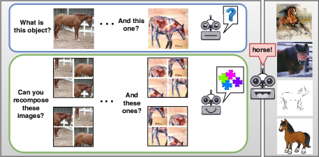
This clear separation between learning intrinsic regularities from images and robust classification across domains is in contrast with the visual learning strategies of biological systems, and in particular of the human visual system. Indeed, numerous studies highlight that infants and toddlers learn both to categorize objects and about regularities at the same time [2]. For instance, popular toys for infants teach to recognize different categories by fitting them into shape sorters; jigsaw puzzles of animals or vehicles to encourage learning of object parts’ spatial relations are equally widespread among 12-18 months old. This type of joint learning is certainly a key ingredient in the ability of humans to reach sophisticated visual generalization abilities at an early age [16].
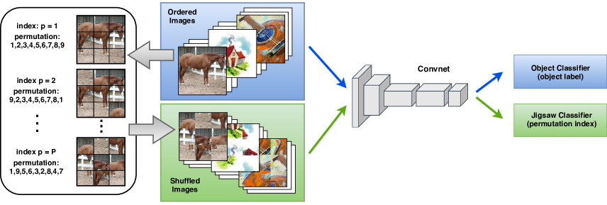
Inspired by this, we propose the first end-to-end architecture that learns simultaneously how to generalize across domains and about spatial co-location of image parts (Figure 1, 2). In this work we focus on the unsupervised task of recovering an original image from its shuffled parts, also known as solving jigsaw puzzles. We show how this popular game can be re-purposed as a side objective to be optimized jointly with object classification over different source domains and improve generalization with a simple multi-task process [7]. We name our Jigsaw puzzle based Generalization method JiGen. Differently from previous approaches that deal with separate image patches and recombine their features towards the end of the learning process [36, 10, 38], we move the patch re-assembly at the image level and we formalize the jigsaw task as a classification problem over recomposed images with the same dimension of the original one. In this way object recognition and patch reordering can share the same network backbone and we can seamlessly leverage over any convolutional learning structure as well as several pretrained models without the need of specific architectural changes.
We demonstrate that JiGen allows to better capture the shared knowledge among multiple sources and acts as a regularization tool for a single source. In the case unlabeled samples of the target data are available at training time, running the unsupervised jigsaw task on them contributes to the feature adaptation process and shows competing results with respect to state of the art unsupervised domain adaptation methods.
2 Related Work
Solving Jigsaw Puzzles
The task of recovering an original image from its shuffled parts is a basic pattern recognition problem that is commonly identified with the jigsaw puzzle game. In the area of computer science and artificial intelligence it was first introduced by [17], which proposed a 9-piece puzzle solver based only on shape information and ignoring the image content. Later, [23] started to make use of both shape and appearance information. The problem has been mainly cast as predicting the permutations of a set of squared patches with all the challenges related to number and dimension of the patches, their completeness (if all tiles are/aren’t available) and homogeneity (presence/absence of extra tiles from other images). The application field for algorithms solving jigsaw puzzles is wide, from computer graphics and image editing [8, 41] to re-compose relics in archaeology [4, 39], from modeling in biology [32] to unsupervised learning of visual representations [15, 36, 10]. Existing assembly strategies can be broadly classified into two main categories: greedy methods and global methods. The first ones are based on sequential pairwise matches, while the second ones search for solutions that directly minimize a global compatibility measure over all the patches. Among the greedy methods, [18] proposed a minimum spanning tree algorithm which progressively merges components while respecting the geometric consistent constraint. To eliminate matching outliers, [42] introduced loop constraints among the patches. The problem can be also formulated as a classification task to predict the relative position of a patch with respect to another as in [15]. Recently, [39] expressed the patch reordering as the shortest path problem on a graph whose structure depends on the puzzle completeness and homogeneity. The global methods consider all the patches together and use Markov Random Field formulations [9], or exploit genetic algorithms [41]. A condition on the consensus agreement among neighbors is used in [43], while [36] focuses on a subset of possible permutations involving all the image tiles and solves a classification problem. The whole set of permutations is instead considered in [10] by approximating the permutation matrix and solving a bi-level optimization problem to recover the right ordering.
Regardless of the specific approach and application, all the most recent deep-learning jigsaw-puzzle solvers tackle the problem by dealing with the separate tiles and then finding a way to recombine them. This implies designing tile-dedicated network architectures then followed by some specific process to transfer the collected knowledge in more standard settings that manage whole image samples.
Domain Generalization and Adaptation
The goal of domain generalization (DG) is that of learning a system that can perform uniformly well across multiple data distributions. The main challenge is being able to distill the most useful and transferrable general knowledge from samples belonging to a limited number of population sources. Several works have reduced the problem to the domain adaptation (DA) setting where a fully labeled source dataset and an unlabeled set of examples from a different target domain are available [11]. In this case the provided target data is used to guide the source training procedure, that however has to run again when changing the application target. To get closer to real world conditions, recent work has started to focus on cases where the source data are drawn from multiple distributions [31, 49] and the target covers only a part of the source classes [5, 1]. For the more challenging DG setting with no target data available at training time, a large part of the previous literature presented model-based strategies to neglect domain specific signatures from multiple sources. They are both shallow and deep learning methods that build over multi-task learning [22], low-rank network parameter decomposition [27] or domain specific aggregation layers [14]. Alternative solutions are based on source model weighting [30], or on minimizing a validation measure on virtual tests defined from the available sources [26]. Other feature-level approaches search for a data representation able to capture information shared among multiple domains. This was formalized with the use of deep learning autoencoders in [20, 28], while [34] proposed to learn an embedding space where images of same classes but different sources are projected nearby. The recent work of [29] adversarially exploits class-specific domain classification modules to cover the cases where the covariate shift assumption does not hold and the sources have different class conditional distributions. Data-level methods propose to augment the source domain cardinality with the aim of covering a larger part of the data space and possibly get closer to the target. This solution was at first presented with the name of domain randomization [44] for samples from simulated environments whose variety was extended with random renderings. In [40] the augmentation is obtained with domain-guided perturbations of the original source instances. Even when dealing with a single source domain, [47] showed that it is still possible to add adversarially perturbed samples by defining fictitious target distributions within a certain Wasserstein distance from the source.
Our work stands in this DG framework, but proposes an orthogonal solution with respect to previous literature by investigating the importance of jointly exploiting supervised and unsupervised inherent signals from the images.
3 The JiGen Approach
Starting from the samples of multiple source domains, we wish to learn a model that can perform well on any new target data population covering the same set of categories. Let us assume to observe domains, with the -th domain containing labeled instances , where indicates the -th image and is its class label. The first basic objective of JiGen is to minimize the loss that measures the error between the true label and the label predicted by the deep model function , parametrized by and . These parameters define the feature embedding space and the final classifier, respectively for the convolutional and fully connected parts of the network. Together with this objective, we ask the network to satisfy a second condition related to solving jigsaw puzzles. We start by decomposing the source images using a regular grid of patches, which are then shuffled and re-assigned to one of the grid positions. Out of the possible permutations we select a set of elements by following the Hamming distance based algorithm in [36], and we assign an index to each entry. In this way we define a second classification task on labeled instances , where indicates the recomposed samples and the related permutation index, for which we need to minimize the jigsaw loss . Here the deep model function has the same structure used for object classification and shares with that the parameters . The final fully connected layer dedicated to permutation recognition is parametrized by . Overall we train the network to obtain the optimal model through
| (1) |
where both and are standard cross-entropy losses. We underline that the jigsaw loss is also calculated on the ordered images. Indeed, the correct patch sorting corresponds to one of the possible permutations and we always include it in the considered subset . On the other way round, the classification loss is not influenced by the shuffled images, since this would make object recognition tougher. At test time we use only the object classifier to predict on the new target images.
Extension to Unsupervised Domain Adaptation
Thanks to the unsupervised nature of the jigsaw puzzle task, we can always extend JiGen to the unlabeled samples of target domain when available at training time. This allows us to exploit the jigsaw task for unsupervised domain adaptation. In this setting, for the target ordered images we minimize the classifier prediction uncertainty through the empirical entropy loss , while for the shuffled target images we keep optimizing the jigsaw loss .
Implementation Details
Overall JiGen 111Code available at https://github.com/fmcarlucci/JigenDG has two parameters related to how we define the jigsaw task, and three related to the learning process. The first two are respectively the grid size used to define the image patches and the cardinality of the patch permutation subset . As we will detail in the following section, JiGen is robust to these values and for all our experiments we kept them fixed, using patch grids and . The remaining parameters are the weights of the jigsaw loss, and assigned to the entropy loss when included in the optimization process for unsupervised domain adaptation. The final third parameter regulates the data input process: the shuffled images enter the network together with the original ordered ones, hence each image batch contains both of them. We define a data bias parameter to specify their relative ratio. For instance means that for each batch, of the images are ordered, while the remaining are shuffled. These last three parameters were chosen by cross validation on a subset of the source images for each experimental setting.
We designed the JiGen network making it able to leverage over many possible convolutional deep architectures. Indeed it is sufficient to remove the existing last fully connected layer of a network and substitute it with the new object and jigsaw classification layers. JiGen is trained with SGD solver, epochs, batch size , learning rate set to and stepped down to after of the training epochs. We used a simple data augmentation protocol by randomly cropping the images to retain between and randomly applied horizontal flipping. Following [38] we randomly ( probability) convert an image tile to grayscale.
4 Experiments
Datasets
To evaluate the performance of JiGen when training over multiple sources we considered three domain generalization datasets. PACS [27] covers object categories and domains (Photo, Art Paintings, Cartoon and Sketches). We followed the experimental protocol in [27] and trained our model considering three domains as source datasets and the remaining one as target. VLCS [45] aggregates images of object categories shared by the PASCAL VOC 2007, LabelMe, Caltech and Sun datasets which are considered as separated domains. We followed the standard protocol of [20] dividing each domain into a training set () and a test set () by random selection from the overall dataset. The Office-Home dataset [46] contains 65 categories of daily objects from 4 domains: Art, Clipart, Product and Real-World. In particular Product images are from vendor websites and show a white background, while Real-World represents object images collected with a regular camera. For this dataset we used the same experimental protocol of [14]. Note that Office-Home and PACS are related in terms of domain types and it is useful to consider both as test-beds to check if JiGen scales when the number of categories changes from 7 to 65. Instead VLCS offers different challenges because it combines object categories from Caltech with scene images of the other domains.
To understand if solving jigsaw puzzles supports generalization even when dealing with a single source, we extended our analysis to digit classification as in [47]. We trained a model on 10k digit samples of the MNIST dataset [25] and evaluated on the respective test sets of MNIST-M [19] and SVHN [35]. To work with comparable datasets, all the images were resized to treated as RGB.
| PACS | art_paint. | cartoon | sketches | photo | Avg. | |
| CFN - Alexnet | ||||||
| J-CFN-Finetune | 47.23 | 62.18 | 58.03 | 70.18 | 59.41 | |
| J-CFN-Finetune++ | 51.14 | 58.83 | 54.85 | 73.44 | 59.57 | |
| C-CFN-Deep All | 59.69 | 59.88 | 45.66 | 85.42 | 62.66 | |
| C-CFN-JiGen | 60.68 | 60.55 | 55.66 | 82.68 | 64.89 | |
| Alexnet | ||||||
| [27] | Deep All | 63.30 | 63.13 | 54.07 | 87.70 | 67.05 |
| TF | 62.86 | 66.97 | 57.51 | 89.50 | 69.21 | |
| [29] | Deep All | 57.55 | 67.04 | 58.52 | 77.98 | 65.27 |
| DeepC | 62.30 | 69.58 | 64.45 | 80.72 | 69.26 | |
| CIDDG | 62.70 | 69.73 | 64.45 | 78.65 | 68.88 | |
| [26] | Deep All | 64.91 | 64.28 | 53.08 | 86.67 | 67.24 |
| MLDG | 66.23 | 66.88 | 58.96 | 88.00 | 70.01 | |
| [14] | Deep All | 64.44 | 72.07 | 58.07 | 87.50 | 70.52 |
| D-SAM | 63.87 | 70.70 | 64.66 | 85.55 | 71.20 | |
| Deep All | 66.68 | 69.41 | 60.02 | 89.98 | 71.52 | |
| JiGen | 67.63 | 71.71 | 65.18 | 89.00 | 73.38 | |
| Resnet-18 | ||||||
| [14] | Deep All | 77.87 | 75.89 | 69.27 | 95.19 | 79.55 |
| D-SAM | 77.33 | 72.43 | 77.83 | 95.30 | 80.72 | |
| Deep All | 77.85 | 74.86 | 67.74 | 95.73 | 79.05 | |
| JiGen | 79.42 | 75.25 | 71.35 | 96.03 | 80.51 | |
 |
 |
 |
|
Patch-Based Convolutional Models for Jigsaw Puzzles
We start our experimental analysis by evaluating the application of existing jigsaw related patch-based convolutional architectures and models to the domain generalization task. We considered two recent works that proposed a jigsaw puzzle solver for 9 shuffled patches from images decomposed by a regular grid. Both [36] and [38] use a Context-Free Network (CFN) with 9 siamese branches that extract features separately from each image patch and then recompose them before entering the final classification layer. Specifically, each CFN branch is an Alexnet [24] up to the first fully connected layer () and all the branches share their weights. Finally, the branches’ outputs are concatenated and given as input to the following fully connected layer (). The jigsaw puzzle task is formalized as a classification problem on a subset of patch permutations and, once the network is trained on a shuffled version of Imagenet [12], the learned weights can be used to initialize the layers of a standard Alexnet while the rest of the network is trained from scratch for a new target task. Indeed, according to the original works, the learned representation is able to capture semantically relevant content from the images regardless of the object labels. We followed the instructions in [36] and started from the pretrained Jigsaw CFN (J-CFN) model provided by the authors to run finetuning for classification on the PACS dataset with all the source domain samples aggregated together. In the top part of Table 1 we indicate with J-CFN-Finetune the results of this experiment using the jigsaw model proposed in [36], while with J-CFN-Finetune++ the results from the advanced model proposed in [38]. In both cases the average classification accuracy on the domains is lower than what can be obtained with a standard Alexnet model pre-trained for object classification on Imagenet and finetuned on all the source data aggregated together. We indicate this baseline approach with Deep All and we can use as reference the corresponding values in the following central part of Table 1. We can conclude that, despite its power as an unsupervised pretext task, completely disregarding the object labels when solving jigsaw puzzles induces a loss of semantic information that may be crucial for generalization across domains.
To demonstrate the potentialities of the CFN architecture, the authors of [36] used it also to train a supervised object Classification model on Imagenet (C-CFN) and demonstrated that it can produce results analogous to the standard Alexnet. With the aim of further testing this network to understand if and how much its peculiar siamese-ennead structure can be useful to distill shared knowledge across domains, we considered it as the main convolutional backbone for JiGen. Starting from the C-CFN model provided by the authors, we ran the obtained C-CFN-JiGen on PACS data, as well as its plain object classification version with the jigsaw loss disabled () that we indicate as C-CFN-Deep All. From the obtained recognition accuracy we can state that combining the jigsaw puzzle with the classification task provides an average improvement in performance, which is the first result to confirm our intuition. However, C-CFN-Deep All is still lower than the reference results obtained with standard Alexnet.
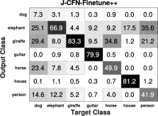
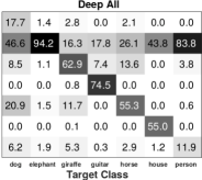
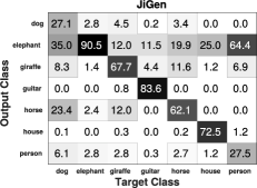
For all the following experiments we consider the convolutional architecture of JiGen built with the same main structure of Alexnet or Resnet, using always the image as a whole (ordered or shuffled) instead of relying on separate patch-based network branches. A detailed comparison of per-class results on the challenging sketches domain for J-CFN-Finetune++ and JiGen based on Alexnet reveals that for four out of seven categories, J-CFN-Finetune++ is actually doing a good job, better than Deep All. With JiGen we improve over Deep All for the same categories by solving jigsaw puzzles at image level and we keep the advantage of Deep All for the remaining categories.
Multi-Source Domain Generalization
We compare the performance of JiGen against several recent domain generalization methods. TF is the low-rank parametrized network that was presented together with the dataset PACS in [27]. CIDDG is the conditional invariant deep domain generalization method presented in [29] that trains for image classification with two adversarial constraints: one that maximizes the overall domain confusion following [19] and a second one that does the same per-class. In the DeepC variant, only this second condition is enabled. MLDG [26] is a meta-learning approach that simulates train/test domain shift during training and exploit them to optimize the learning model. CCSA [34] learns an embedding subspace where mapped visual domains are semantically aligned and yet maximally separated. MMD-AAE [28] is a deep method based on adversarial autoencoders that learns an invariant feature representation by aligning the data distributions to an arbitrary prior through the Maximum Mean Discrepancy (MMD). SLRC [13] is based on a single domain invariant network and multiple domain specific ones and it applies a low rank constraint among them. D-SAM [14] is a method based on the use of domain-specific aggregation modules combined to improve model generalization: it provides the current sota results on PACS and Office-Home. For each of these methods, the Deep All baseline indicates the performance of the corresponding network when all the introduced domain adaptive conditions are disabled.
| VLCS | Caltech | Labelme | Pascal | Sun | Avg. | |
| Alexnet | ||||||
| [29] | Deep All | 85.73 | 61.28 | 62.71 | 59.33 | 67.26 |
| DeepC | 87.47 | 62.60 | 63.97 | 61.51 | 68.89 | |
| CIDDG | 88.83 | 63.06 | 64.38 | 62.10 | 69.59 | |
| [34] | Deep All | 86.10 | 55.60 | 59.10 | 54.60 | 63.85 |
| CCSA | 92.30 | 62.10 | 67.10 | 59.10 | 70.15 | |
| [13] | Deep All | 86.67 | 58.20 | 59.10 | 57.86 | 65.46 |
| SLRC | 92.76 | 62.34 | 65.25 | 63.54 | 70.97 | |
| [27] | Deep All | 93.40 | 62.11 | 68.41 | 64.16 | 72.02 |
| TF | 93.63 | 63.49 | 69.99 | 61.32 | 72.11 | |
| [28] | MMD-AAE | 94.40 | 62.60 | 67.70 | 64.40 | 72.28 |
| [14] | Deep All | 94.95 | 57.45 | 66.06 | 65.87 | 71.08 |
| D-SAM | 91.75 | 56.95 | 58.59 | 60.84 | 67.03 | |
| Deep All | 96.93 | 59.18 | 71.96 | 62.57 | 72.66 | |
| JiGen | 96.93 | 60.90 | 70.62 | 64.30 | 73.19 | |
| Office-Home | Art | Clipart | Product | Real-World | Avg. | |
|---|---|---|---|---|---|---|
| Resnet-18 | ||||||
| [14] | Deep All | 55.59 | 42.42 | 70.34 | 70.86 | 59.81 |
| D-SAM | 58.03 | 44.37 | 69.22 | 71.45 | 60.77 | |
| Deep All | 52.15 | 45.86 | 70.86 | 73.15 | 60.51 | |
| JiGen | 53.04 | 47.51 | 71.47 | 72.79 | 61.20 | |
 |
 |
 |
 |
The central and bottom parts of Table 1 show the results of JiGen on the dataset PACS when using as backbone architecture Alexnet and Resnet-18222With Resnet18, to put JiGen on equal footing with D-SAM we follow the same data augmentation protocol in [14] and enabled color jittering.. On average JiGen produces the best result when using Alexnet and it is just slightly worse than the D-SAM reference for Resnet-18. Note however, that in this last case, JiGen outperforms D-SAM in three out of four target cases and the average advantage of D-SAM originate only from its result on sketches. On average, JiGen outperforms also the competing methods on the VLCS and on the Office-Home datasets (see respectively Table 2 and 3). In particular we remark that VLCS is a tough setting where the most recent works have only presented small gain in accuracy with respect to the corresponding Deep All baseline (e.g. TF). Since [14] did not present the results of D-SAM on the VLCS dataset, we used the code provided by the authors to run these experiments. The obtained results show that, although generally able to close large domain gaps across images of different styles as in PACS and Office-Home, when dealing with domains all coming from real-world images, the use of aggregative modules does not support generalization.
 |
 |
Ablation
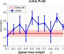
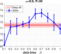
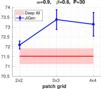
We focus on the Alexnet-PACS DG setting for an ablation analysis on the respective roles of the jigsaw and of the object classification task in the learning model. For these experiments we kept the jigsaw hyperparameters fixed with a patch grid and jigsaw classes. means that the jigsaw task is off, and the data batches contain only original ordered images, which corresponds to Deep All. The value assigned to the data bias drives the overall training: it moves the focus from jigsaw when using low values () to object classification when using high values (). By setting the data bias to we feed the network with more ordered than shuffled images, thus keeping the classification as the primary goal of the network. In this case, when changing the jigsaw loss weight in , we observe results which are always either statistically equal or better than the Deep All baseline as shown in the first plot of Figure 4. The second plot indicates that, for high values of , tuning has a significant effect on the overall performance. Indeed means that jigsaw task is on and highly relevant in the learning process, but we are feeding the network only with ordered images: in this case the jigsaw task is trivial and forces the network to recognize always the same permutation class which, instead of regularizing the learning process, may increase the risk of data memorization and overfitting. Further experiments confirm that, for but lower values, JiGen and Deep All perform equally well. Setting means feeding the network only with shuffled images. For each image we have variants, only one of which has the patches in the correct order and is allowed to enter the object classifier, resulting in a drastic reduction of the real batch size. In this condition the object classifier is unable to converge, regardless of whether the jigsaw classifier is active () or not (). In those cases the accuracy is very low (), so we do not show it in the plots to ease the visualization.
Jigsaw hyperparameter tuning
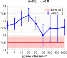
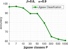
By using the same experimental setting of the previous paragraph, the third plot in Figure 4 shows the change in performance when the number of jigsaw classes varies between 5 and 1000. We started from a low number, with the same order of magnitude of the number of object classes in PACS, and we grew till 1000 which is the number used for the experiments in [36]. We observe an overall variation of 1.5 percentage points in the accuracy which still remains (almost always) higher than the Deep All baseline. Finally, we ran a test to check the accuracy when changing the grid size and consequently the patch number. Even in this case, the range of variation is limited when passing from a to a grid, confirming the conclusions of robustness already obtained for this parameter in [36] and [10]. Moreover all the results are better than the Deep All reference.
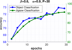
It is also interesting to check whether the jigsaw classifier is producing meaningful results per-se, besides supporting generalization for the object classifier. We show its recognition accuracy when testing on the same images used to evaluate the object classifier but with shuffled patches. In Figure 5, the first plot shows the accuracy over the learning epochs for the object and jigsaw classifiers indicating that both grows simultaneously (on different scales). The second plot shows the jigsaw recognition accuracy when changing the number of permutation classes : of course the performance decreases when the task becomes more difficult, but overall the obtained results indicate that the jigsaw model is always effective in reordering the shuffled patches.
Single Source Domain Generalization
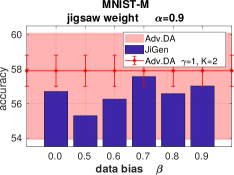
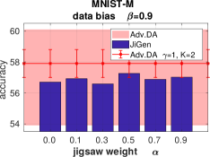
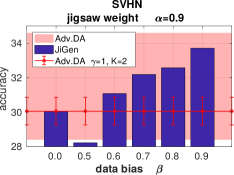
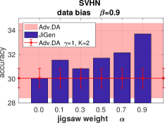
The generalization ability of a model depends both on the chosen learning process and on the used training data. To investigate the former and better evaluate the regularization effect provided by the jigsaw task, we consider the case of training data from a single source domain. For these experiments we compare against the generalization method based on adversarial data augmentation (Adv.DA) recently presented in [47]. This work proposes an iterative procedure that perturbs the samples to make them hard to recognize under the current model and then combine them with the original ones while solving the classification task. We reproduced the experimental setting used in [47] and adopt a similar result display style with bar plots for experiments on the MNIST-M and SVHN target datasets when training on MNIST. In Figure 6 we show the performance of JiGen when varying the data bias and the jigsaw weight . With the red background shadow we indicate the overall range covered by Adv.DA results when changing its parameters333The whole set of results is provided as supplementary material of [47]., while the horizontal line is the reference Adv.DA results around which the authors of [47] ran their parameter ablation analysis. The figure indicates that, although Adv.DA can reach high peak values, it is also very sensitive to the chosen hyperparameters. On the other hand, JiGen is much more stable and it is always better than the lower accuracy value of Adv.DA with a single exception for SVHN and data bias 0.5, but we know from the ablation analysis, that this corresponds to a limit case for the proper combination of object and jigsaw classification. Moreover, JiGen gets close to Adv.DA reference results for MNIST-M and significantly outperform it for SVHN.
| PACS-DA | art_paint. | cartoon | sketches | photo | Avg. | |
| Resnet-18 | ||||||
| [31] | Deep All | 74.70 | 72.40 | 60.10 | 92.90 | 75.03 |
| Dial | 87.30 | 85.50 | 66.80 | 97.00 | 84.15 | |
| DDiscovery | 87.70 | 86.90 | 69.60 | 97.00 | 85.30 | |
| Deep All | 77.85 | 74.86 | 67.74 | 95.73 | 79.05 | |
| JiGen | 84.88 | 81.07 | 79.05 | 97.96 | 85.74 | |
| JiGen | 85.58 | 82.18 | 78.61 | 98.26 | 86.15 | |
| JiGen | 85.08 | 81.28 | 81.50 | 97.96 | 86.46 | |
| JiGen | 85.73 | 82.58 | 78.34 | 98.10 | 86.19 | |
| JiGen | 85.32 | 80.56 | 79.93 | 97.63 | 85.86 | |
Unsupervised Domain Adaptation
When unlabeled target samples are available at training time we can let the jigsaw puzzle task involve these data. Indeed patch reordering does not need image labels and running the jigsaw optimization process on both source and target data may positively influence the source classification model for adaptation. To verify this intuition we considered again the PACS dataset and used it in the same unsupervised domain adaptation setting of [31]. This previous work proposed a method to first discover the existence of multiple latent domains in the source data and then differently adapt their knowledge to the target depending on their respective similarity. It has been shown that this domain discovery (DDiscovery) technique outperforms other powerful adaptive approaches as Dial [6] when the source actually includes multiple domains. Both these methods exploit the minimization of the entropy loss as an extra domain alignment condition: in this way the source model when predicting on the target samples is encouraged to assign maximum prediction probability to a single label rather than distributing it over multiple class options. For a fair comparison we also turned on the entropy loss for JiGen with weight . Moreover, we considered two cases for the jigsaw loss: either keeping the weight already used for the PACS-Resnet-18 DG experiments for both the source and target data (), or treating the domain separately with a dedicated weight for the jigsaw target loss (, ). The results for this setting are summarized in Table 4. The obtained accuracy indicates that JiGen outperforms the competing methods on average and in particular on the difficult task of recognizing sketches. Furthermore, the advantage remains true regardless of the specific choice of the target jigsaw loss weight.
5 Conclusions
In this paper we showed for the first time that generalization across visual domains can be achieved effectively by learning to classify and learning intrinsic image invariances at the same time. We focused on learning spatial co-location of image parts, and proposed a simple yet powerful framework that can accommodate a wide spectrum of pre-trained convolutional architectures. Our method JiGen can be seamlessly and effectively used for domain adaptation and generalization as shown by the experimental results.
We see this paper as opening the door to a new research thread in domain adaptation and generalization. While here we focused on a specific type of invariance, several other regularities could be learned possibly leading to an even stronger benefit. Also, the simplicity of our approach calls for testing its effectiveness in applications different from object categorization, like semantic segmentation and person re-identification, where the domain shift effect strongly impact the deployment of methods in the wild.
Acknowledgments
This work was supported by the ERC grant 637076 RoboExNovo and a NVIDIA Academic Hardware Grant.
Appendix A Appendix
We provide here some further analysis and experimental results on using jigsaw puzzle and other self-supervised tasks as auxiliary objectives to improve generalization across visual domains.
Visual explanation and Failure cases
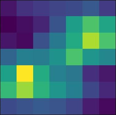
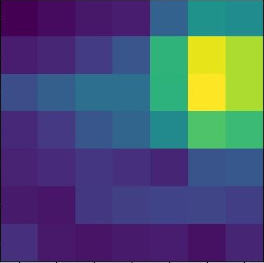
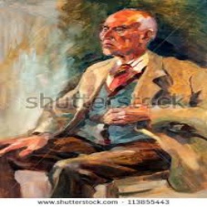
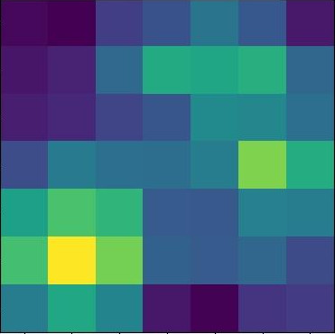
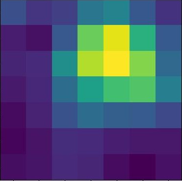
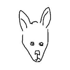
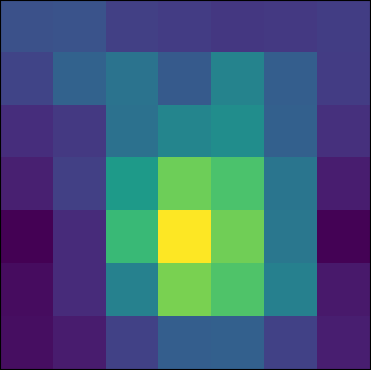
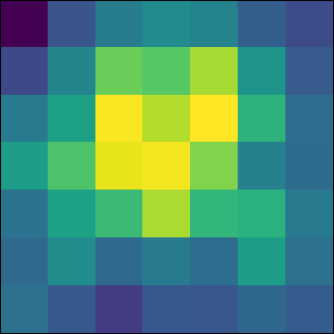
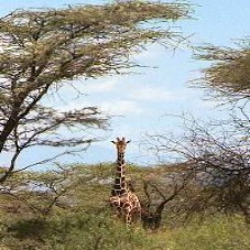
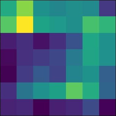
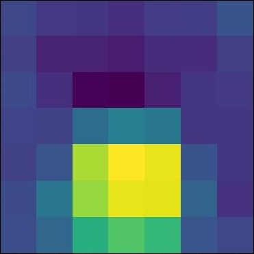
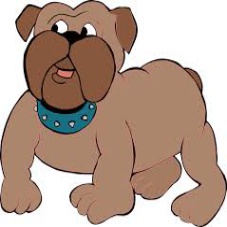
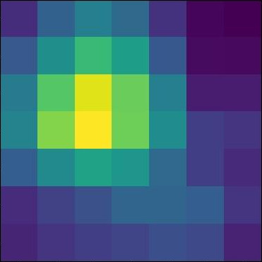
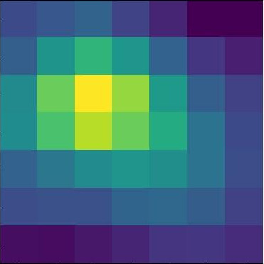
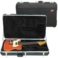
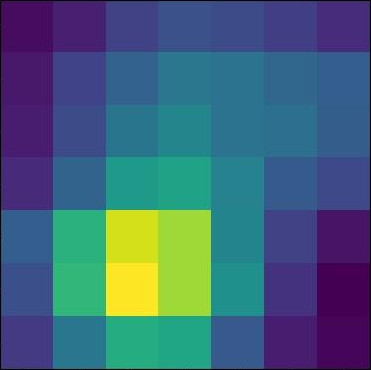
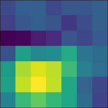
The relative position of each image patch with respect to the others captures visual regularities which are at the same time shared among domains and discriminative with respect to the object classes. Thus, by solving jigsaw puzzles we encourage the network to localize and re-join relevant object sub-parts regardless of the visual domain. This helps to focus on the most informative image areas. For an in-depth analysis of the learned model we adopted the Class Activation Mapping (CAM, [51]) method on ResNet-18, with which we produced the activation maps in Figure 7 for the PACS dataset. The first two rows show that JiGen is better at localizing the object class with respect to Deep All. The last row indicates that the mistakes are related to some flaw in data interpretation, while the localization remains correct.
Self-supervision by predicting image rotations
Reordering image patches to solve jigsaw puzzle is not the only self-supervised approach that can be combined with supervised learning for domain generalization. We ran experiments by using as auxiliary self-supervised task the rotation classifier (four classes ) proposed in [21]. We focused on the PACS dataset with the Alexnet-based architecture, following the same protocol used for JiGen. The obtained accuracy (Table 5) is higher than the Deep All baseline, but still lower than what obtained with our method. Indeed object 2d orientation provides useful semantic information when dealing with real photos, but it becomes less critical for cartoons and sketches.
| Deep All ✗ | JiGen ✓ | Deep All ✗ | JiGen ✓ | ||
 |
 |
 |
 |
 |
 |
 |
 |
 |
 |
 |
 |
| Deep All ✓ | JiGen ✗ | Deep All ✓ | JiGen ✗ | ||
 |
 |
 |
 |
 |
 |
| PACS | art_paint. | cartoon | sketches | photo | Avg. | |
|---|---|---|---|---|---|---|
| Alexnet | ||||||
| Deep All | 66.68 | 69.41 | 60.02 | 89.98 | 71.52 | |
| Rotation | 67.67 | 69.83 | 61.04 | 89.98 | 72.13 | |
| JiGen | 67.63 | 71.71 | 65.18 | 89.00 | 73.38 | |
![[Uncaptioned image]](/html/1903.06864/assets/figures_map/pic_167.jpg) |
![[Uncaptioned image]](/html/1903.06864/assets/figures_map/pic_314.jpg) |
![[Uncaptioned image]](/html/1903.06864/assets/figures_map/pic_346.jpg) |
![[Uncaptioned image]](/html/1903.06864/assets/figures_map/7370.png) |
![[Uncaptioned image]](/html/1903.06864/assets/figures_map/n02503517_1852-1.png) |
![[Uncaptioned image]](/html/1903.06864/assets/figures_map/12087.png) |
References
- [1] Gabriele Angeletti, Barbara Caputo, and Tatiana Tommasi. Adaptive deep learning through visual domain localization. In International Conference on Robotic Automation (ICRA), 2018.
- [2] Jeffrey Bisanz, Gay L. Bisanz, and Robert Kail, editors. Learning in Children: Progress in Cognitive Development Research. Springer-Verlag, 1983.
- [3] Konstantinos Bousmalis, George Trigeorgis, Nathan Silberman, Dilip Krishnan, and Dumitru Erhan. Domain Separation Networks. In Neural Information Processing Systems (NIPS), 2016.
- [4] Benedict J. Brown, Corey Toler-Franklin, Diego Nehab, Michael Burns, David Dobkin, Andreas Vlachopoulos, Christos Doumas, Szymon Rusinkiewicz, and Tim Weyrich. A system for high-volume acquisition and matching of fresco fragments: Reassembling Theran wall paintings. ACM Transactions on Graphics (Proc. SIGGRAPH), 27(3), Aug. 2008.
- [5] Zhangjie Cao, Lijia Ma, Mingsheng Long, and Jianmin Wang. Partial adversarial domain adaptation. In Europeran Conference on Computer Vision (ECCV), 2018.
- [6] Fabio Maria Carlucci, Lorenzo Porzi, Barbara Caputo, Elisa Ricci, and Samuel Rota Bulò. Just dial: domain alignment layers for unsupervised domain adaptation. In International Conference on Image Analysis and Processing (ICIAP), 2017.
- [7] Rich Caruana. Multitask learning. Mach. Learn., 28(1):41–75, 1997.
- [8] Taeg Sang Cho, Shai Avidan, and William T. Freeman. The patch transform. IEEE Transactions on Pattern Analysis & Machine Intelligence, 32:1489–1501, 2009.
- [9] Taeg Sang Cho, Shai Avidan, and William T. Freeman. A probabilistic image jigsaw puzzle solver. In Computer Vision and Pattern Recognition (CVPR), 2010.
- [10] Rodrigo Santa Cruz, Basura Fernando, Anoop Cherian, and Stephen Gould. Visual permutation learning. In Computer Vision and Pattern Recognition (CVPR), 2017.
- [11] Gabriela Csurka, editor. Domain Adaptation in Computer Vision Applications. Advances in Computer Vision and Pattern Recognition. Springer, 2017.
- [12] Jia Deng, Wei Dong, Richard Socher, Li jia Li, Kai Li, and Li Fei-Fei. Imagenet: A large-scale hierarchical image database. In Conference on Computer Vision and Pattern Recognition (CVPR), 2009.
- [13] Zhengming Ding and Yun Fu. Deep domain generalization with structured low-rank constraint. IEEE Transactions on Image Processing, 27:304–313, 2017.
- [14] Antonio D’Innocente and Barbara Caputo. Domain generalization with domain-specific aggregation modules. In German Conference on Pattern Recognition (GCPR), 2018. Code available at https://github.com/VeloDC/D-SAM_public.
- [15] Carl Doersch, Abhinav Gupta, and Alexei A. Efros. Unsupervised visual representation learning by context prediction. In International Conference on Computer Vision (ICCV), 2015.
- [16] Brock Ferguson, Steven L. Franconeri, and Sandra R. Waxman. Very young infants learn abstract rules in the visual modality. PLOS ONE, 13(1):1–14, 01 2018.
- [17] Herbert Freeman and L. Garder. Apictorial jigsaw puzzles: The computer solution of a problem in pattern recognition. IEEE Trans. Electronic Computers, 13(2):118–127, 1964.
- [18] Andrew C. Gallagher. Jigsaw puzzles with pieces of unknown orientation. In Computer Vision and Pattern Recognition (CVPR), 2012.
- [19] Yaroslav Ganin, Evgeniya Ustinova, Hana Ajakan, Pascal Germain, Hugo Larochelle, François Laviolette, Mario Marchand, and Victor Lempitsky. Domain-adversarial training of neural networks. J. Mach. Learn. Res., 17(1):2096–2030, 2016.
- [20] Muhammad Ghifary, W. Bastiaan Kleijn, Mengjie Zhang, and David Balduzzi. Domain generalization for object recognition with multi-task autoencoders. In International Conference on Computer Vision, (ICCV), 2015.
- [21] Spyros Gidaris, Praveer Singh, and Nikos Komodakis. Unsupervised representation learning by predicting image rotations. In International Conference on Learning Representations (ICLR), 2018.
- [22] Aditya Khosla, Tinghui Zhou, Tomasz Malisiewicz, Alexei Efros, and Antonio Torralba. Undoing the damage of dataset bias. In European Conference on Computer Vision (ECCV), 2012.
- [23] David A. Kosiba, Pierre M. Devaux, Sanjay Balasubramanian, Tarak Gandhi, and Rangachar Kasturi. An automatic jigsaw puzzle solver. In International Conference on Pattern Recognition (ICPR), 1994.
- [24] Alex Krizhevsky, Ilya Sutskever, and Geoffrey E Hinton. Imagenet classification with deep convolutional neural networks. In Advances in Neural Information Processing Systems (NIPS), 2012.
- [25] Yann LeCun, Léon Bottou, Yoshua Bengio, and Patrick Haffner. Gradient-based learning applied to document recognition. Proceedings of the IEEE, 86(11):2278–2324, 1998.
- [26] Da Li, Yongxin Yang, Yi-Zhe Song, and Timothy M. Hospedales. Learning to generalize: Meta-learning for domain generalization. In Conference of the Association for the Advancement of Artificial Intelligence (AAAI), 2018.
- [27] Da Li, Yongxin Yang, Yi-Zhe Song, and Timothy M. Hospedales. Deeper, broader and artier domain generalization. In International Conference on Computer Vision (ICCV), 2017.
- [28] Haoliang Li, Sinno Jialin Pan, Shiqi Wang, and Alex C. Kot. Domain generalization with adversarial feature learning. In Computer Vision and Pattern Recognition (CVPR), 2018.
- [29] Ya Li, Xinmei Tian, Mingming Gong, Yajing Liu, Tongliang Liu, Kun Zhang, and Dacheng Tao. Deep domain generalization via conditional invariant adversarial networks. In The European Conference on Computer Vision (ECCV), September 2018.
- [30] Massimiliano Mancini, Samuel Rota Bulo, Barbara Caputo, and Elisa Ricci. Robust place categorization with deep domain generalization. IEEE Robotics and Automation Letters, 2018.
- [31] Massimilano Mancini, Lorenzo Porzi, Samuel Rota Bulò, Barbara Caputo, and Elisa Ricci. Boosting domain adaptation by discovering latent domains. In Computer Vision and Pattern Recognition (CVPR), 2018.
- [32] William Marande and Gertraud Burger. Mitochondrial dna as a genomic jigsaw puzzle. Science, 318(5849):415–415, 2007.
- [33] Ishan Misra, C. Lawrence Zitnick, and Martial Hebert. Shuffle and Learn: Unsupervised Learning using Temporal Order Verification. In European Conference on Computer Vision (ECCV), 2016.
- [34] Saeid Motiian, Marco Piccirilli, Donald A. Adjeroh, and Gianfranco Doretto. Unified deep supervised domain adaptation and generalization. In International Conference on Computer Vision (ICCV), 2017.
- [35] Yuval Netzer, Tao Wang, Adam Coates, Alessandro Bissacco, Bo Wu, and Andrew Y. Ng. Reading digits in natural images with unsupervised feature learning. In NIPS workshop on deep learning and unsupervised feature learning, 2011.
- [36] Mehdi Noroozi and Paolo Favaro. Unsupervised learning of visual representations by solving jigsaw puzzles. In European Conference on Computer Vision (ECCV), 2016.
- [37] Mehdi Noroozi, Hamed Pirsiavash, and Paolo Favaro. Representation learning by learning to count. In International Conference on Computer Vision (ICCV), 2017.
- [38] Mehdi Noroozi, Ananth Vinjimoor, Paolo Favaro, and Hamed Pirsiavash. Boosting self-supervised learning via knowledge transfer. In Conference on Computer Vision and Pattern Recognition (CVPR), 2018.
- [39] Marie-Morgane Paumard, David Picard, and Hedi Tabia. Image reassembly combining deep learning and shortest path problem. In European Conference on Computer Vision (ECCV), 2018.
- [40] Shiv Shankar, Vihari Piratla, Soumen Chakrabarti, Siddhartha Chaudhuri, Preethi Jyothi, and Sunita Sarawagi. Generalizing across domains via cross-gradient training. In International Conference on Learning Representations (ICLR), 2018.
- [41] Dror Sholomon, Omid E. David, and Nathan S. Netanyahu. A generalized genetic algorithm-based solver for very large jigsaw puzzles of complex types. In Conference on Artificial Intelligence (AAAI), 2014.
- [42] Kilho Son, James Hays, and David B. Cooper. Solving square jigsaw puzzles with loop constraints. In European Conference on Computer Vision (ECCV), 2014.
- [43] Kilho Son, Daniel Moreno, James Hays, and David B. Cooper. Solving small-piece jigsaw puzzles by growing consensus. In Computer Vision and Pattern Recognition (CVPR), 2016.
- [44] Joshua Tobin, Rachel Fong, Alex Ray, Jonas Schneider, Wojciech Zaremba, and Pieter Abbeel. Domain randomization for transferring deep neural networks from simulation to the real world. In International Conference on Intelligent Robots and Systems (IROS), 2017.
- [45] Antonio Torralba and Alexei A. Efros. Unbiased look at dataset bias. In Conference on Computer Vision and Pattern Recognition (CVPR), 2011.
- [46] Hemanth Venkateswara, Jose Eusebio, Shayok Chakraborty, and Sethuraman Panchanathan. Deep hashing network for unsupervised domain adaptation. In Conference on Computer Vision and Pattern Recognition (CVPR), 2017.
- [47] Riccardo Volpi, Hongseok Namkoong, Ozan Sener, John Duchi, Vittorio Murino, and Silvio Savarese. Generalizing to unseen domains via adversarial data augmentation. In Neural Information Processing Systems (NIPS), 2018.
- [48] Xiaolong Wang and Abhinav Gupta. Unsupervised learning of visual representations using videos. In International Conference on Computer Vision (ICCV), 2015.
- [49] Ruijia Xu, Ziliang Chen, Wangmeng Zuo, Junjie Yan, and Liang Lin. Deep cocktail network: Multi-source unsupervised domain adaptation with category shift. In Computer Vision and Pattern Recognition (CVPR), 2018.
- [50] Richard Zhang, Phillip Isola, and Alexei A Efros. Colorful image colorization. In European Conference on Computer Vision (ECCV), 2016.
- [51] Bolei Zhou, Aditya Khosla, Agata Lapedriza, Aude Oliva, and Antonio Torralba. Learning deep features for discriminative localization. In Conference on Computer Vision and Pattern Recognition (CVPR), 2016.