Learning Super-resolution 3D Segmentation of Plant Root MRI Images from Few Examples

Abstract

Analyzing plant roots is crucial to understand plant performance in different soil environments. While magnetic resonance imaging (MRI) can be used to obtain 3D images of plant roots, extracting the root structural model is challenging due to highly noisy soil environments and low-resolution of MRI images. To improve both contrast and resolution, we adapt the state-of-the-art method RefineNet for 3D segmentation of the plant root MRI images in super-resolution. The networks are trained from few manual segmentations that are augmented by geometric transformations, realistic noise, and other variabilities. The resulting segmentations contain most root structures, including branches not extracted by the human annotator.

1 Introduction

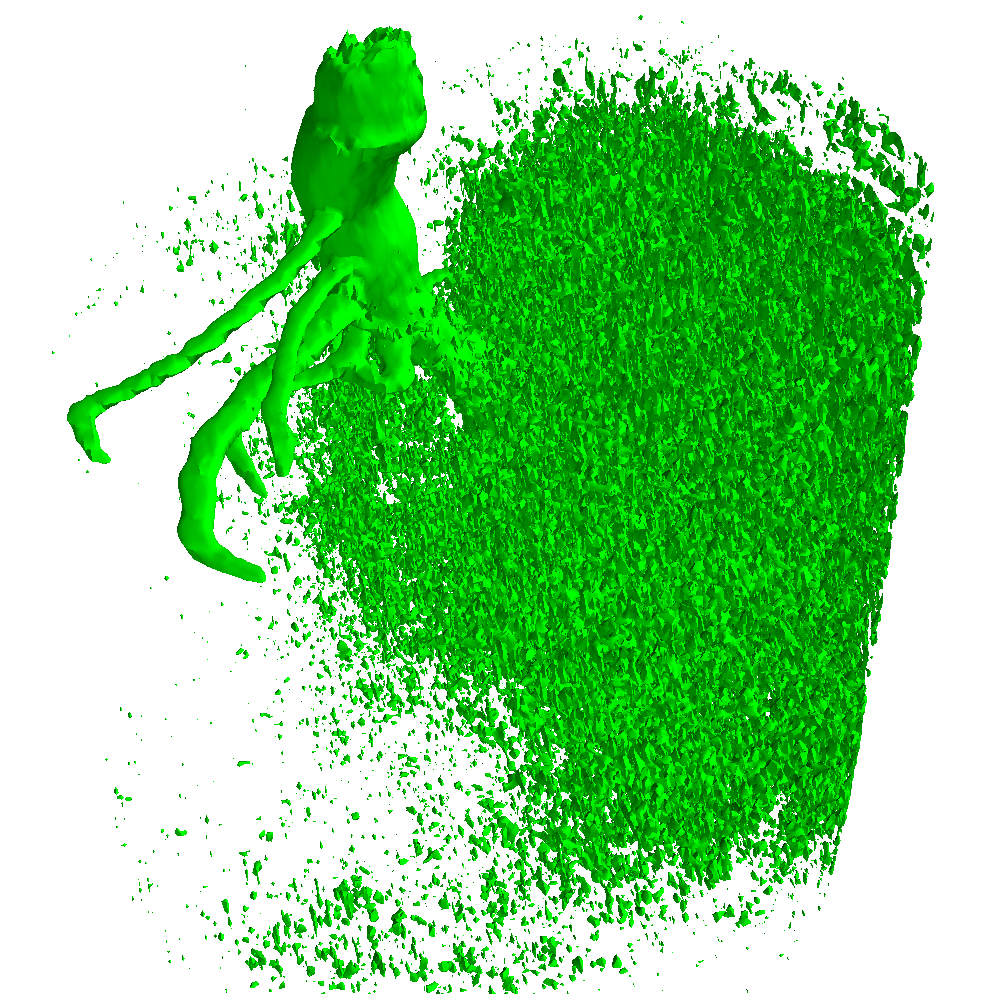
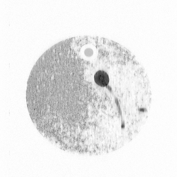
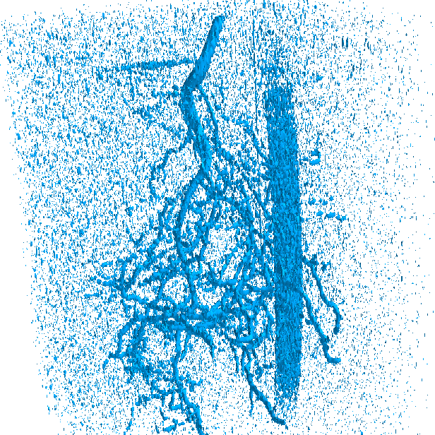
Plant roots have been a long-standing research topic due to their crucial role for plants [1]. Their analysis requires extracting the root structural model. To that end, 3D measurements of plant roots in opaque soil are obtained with MRI (Figure 1) for use in root model extraction algorithms [1, 2, 3]. Often, the soil is noisy and the resolution of MRI images is too low to capture thin roots with precision, resulting in low signal-to-noise ratio (SNR). With low SNR, automated extraction of root structural models is challenging [2], requiring a preprocessing step to reduce the noise and increase the resolution artificially. In recent years, deep learning methods have shown great success with many computer vision tasks such as image classification [4], action detection [5], and semantic segmentation [6]. To improve both contrast and resolution of MRI, we adapt the state-of-the-art transfer learning method RefineNet [6] for 3D, super-resolution segmentation of plant root MRI images as root vs non-root. Since the original data we were provided with is insufficient for training, we generate our own synthetic training data from reconstructed root structures.

Figure 1: First two images depict the 3D visualization and a single slice from Root 1. Third and fourth images depict the 3D visualization and a single slice (contrast enhanced & magnified) from Root 2.

2 Related Work

Recent deep learning methods define the state-of-the-art results for semantic segmentation [6, 7]. Using a technique known as transfer learning, the features learned from large data sets are leveraged to initialize training on a small, related data set, resulting in shorter training times and less need for training data.

Despite extensive work on semantic segmentation for 3D medical data, the use of 3D CNNs remains limited due to high memory and computational power requirements of training. For example, a 3D CNN is proposed by [8] [8] for skull stripping from MRI images. However, the dataset is rather small and the resulting segmentations have lower resolution than the network input.

2D CNNs can also be utilized for segmentation of 3D data. A 2D CNN by [9] [9] achieves comparable results to the state-of-the-art results at brain tumor segmentation from MRI images.

In addition to semantic segmentation, deep learning methods also define state-of-the-art results for super-resolution. Usually, the mapping from low-resolution to a higher resolution is done by incorporating upsampling [10], transposed convolutional layers [11], or serialization [12].

[1, 2] [1, 2] introduce algorithms for automated structural model extraction from MRI root images, yet, these algorithms do not perform well on MRI images with low SNR. Using 3D CNNs, an attempt to increase the SNR by 3D segmentation of MRI images has been made by [13] [13]. While accurate results can be obtained, higher memory consumption and longer training times prevent the construction of deep architectures. Moreover, training is difficult as the networks are highly volatile to parameterizations of learning rate, kernel size, number of channels, and number of layers.

3 Segmentation Method

To increase the resolution, we target super-resolution factor $k=2$, i.e., mapping from an input image $I\in\mathbb{R}^{x\times y\times z}$ to a binary segmentation $S\in B^{2x\times 2y\times 2z}$. The non-root and root voxels are denoted with 0 and 1, respectively. We label the axis that follows the plant root from top to the bottom as $z$ while the other two axes are labeled with $x$ and $y$. A layer is referred to a single slice of 1 voxel thickness on the $z$ axis.

It has been reported that 2D CNNs can generate accurate segmentations of 3D data [9]. Encouraged by the benefits of transfer learning [14] and state-of-the-art results of the RefineNet [6], we adapt 2D RefineNet for 3D segmentation of plant root MRI images in super-resolution. We apply 2D segmentation on each layer of the MRI image and obtain two consecutive segmented layers on the $z$ axis that have twice the resolution of the input in both $x$ and $y$ axes.

3.1 RefineNet

RefineNet [6] exploits both high and low-level features of the pretrained networks by introducing RefineNet blocks. Through these blocks, feature maps with different resolutions are fused together to produce high-resolution outputs. [6] [6] cascade RefineNet blocks for best performance. We extend the original 4-Cascade RefineNet architecture [6] to construct 7-Cascade RefineNet (Figure 2) for image segmentation.

Figure 2: 7-Cascade RefineNet. Includes figures from [6] [6].

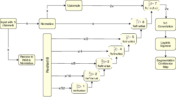
We apply the segmentations layer-wise. Since 3D information must also be exploited, for segmentation of each single layer, we use the layer itself and its four neighboring layers. Extracting features from ResNet requires 2D RGB images, thus, these five layers must be mapped to three channels. To compress the data into three channels while retaining maximum information, PCA is used. The first, second, and the third components of PCA are mapped to green, red, and blue respectively; according to the contribution of each channel into image luminance.

The cascaded RefineNet blocks are shown in Figure 2. As in the original 4-Cascade RefineNet [6], the resolution on both $x$ and $y$ axes are increased by a factor of two at each block. To achieve a super-resolution factor of two, we add three more blocks. Features that are extracted from five different stages of ResNet are fed to blocks 1–5. The remaining blocks 6 & 7 operate on the original and super-resolution inputs. As they do not use the activations of ResNet, mapping to RGB is skipped; the original five layers of input are utilized directly by interpreting these layers as the channels of the network input. The 7th RefineNet block is followed by a $1\times 1$ convolutional layer outputting two channels. Through the use of the logistic sigmoid function, the two channels are interpreted as two consecutive predicted layers where the voxel values denote the confidence of the network that the voxel belongs to a root.

3.2 Data Augmentation and Training

We were provided with four MRI root images and their manual root structure reconstruction. From the root structure, ground truth for the MRI images can be generated by voxelization. As the generated root voxels do not align well with the root structures in the MRI images, we cannot use real MRI images for training with the generated ground truth, though. We address this issue by generating artificial MRI images with perfectly aligned ground truth. Variety is introduced with transformations such as thickness adjustment, rotation, mirroring etc. Modeled after the MRI images in Fig. 1, we generate soil noise in different intensity scales using Perlin noise, uniformly and normally distributed noise for artificial MRI images. We use 384 artificial MRI–ground truth pairs for training and 384 for validation. The network is trained for 100 epochs with learning rate 6e-4 and gradient clipping 0.01 on artificial training pairs.

3.3 Evaluation

Only a small fraction of the number of voxels actually contain root, thus, F1-Score is used as a metric for robustness against class imbalance. On augmented data, we calculate the average F1-Score on the whole validation set. Moreover, the overall F1-Score for a given SNR range is also calculated.

The provided manual root annotations often contain misalignments with the real MRI images. We introduce a Distance Tolerant F1-Score for robustness against such small differences. To this end, we define distance tolerant precision $p^{\prime}$ and recall $r^{\prime}$ as follows:

$$p^{\prime}=\frac{\sum_{i,j,k=0}^{\hat{x},\hat{y},\hat{z}}dilate(G,d)^{i,j,k}\cdot S^{i,j,k}}{\sum_{i,j,k=0}^{\hat{x},\hat{y},\hat{z}}S^{i,j,k}}\text{,} r^{\prime}=\frac{\sum_{i,j,k=0}^{\hat{x},\hat{y},\hat{z}}{G}^{i,j,k}\cdot dilate({S},d)^{i,j,k}}{\sum_{i,j,k=0}^{\hat{x},\hat{y},\hat{z}}G^{i,j,k}}$$

where $G,S\in\mathbb{B}^{\hat{x},\hat{y},\hat{z}}$ are ground truth and predicted segmentation, respectively. Given a distance tolerance $d$, $dilate(I,d)$ refers to a morphological dilation of binary image $I$ by $d$ voxels. Using $p^{\prime}$ and $r^{\prime}$, F1-Score is calculated as usual.

Figure 3: Segmentation performance on the augmented data validation set.

4 Results

We evaluate our method on both synthetic (validation set) and real (test set) MRI data. The results on the validation set are presented in Fig. 3. Compared to the mean F1-Score 0.84 of [13] [13], ours is much better: 0.95. We further train a RefineNet architecture with the transfer learning layers removed; the average F1-Score drops from 0.95 to 0.91. For SNR lower than 3.16, the average F1-Score is 0.84 compared to 0.89 of the original; the remaining SNR ranges do not show much difference. The network is further tested on two real root MRI images using distance tolerant F1-Score (Figure 4). The results indicate that most roots are reconstructed correctly. The super-resolution contours of the segmented roots are detailed and smooth. Our method even detects additional roots not reconstructed by the human annotator, which are counted as false positives. For Root 2, our method is sensitive to elongated MRI artifacts, which have not been present in the synthetic training data.

Root 1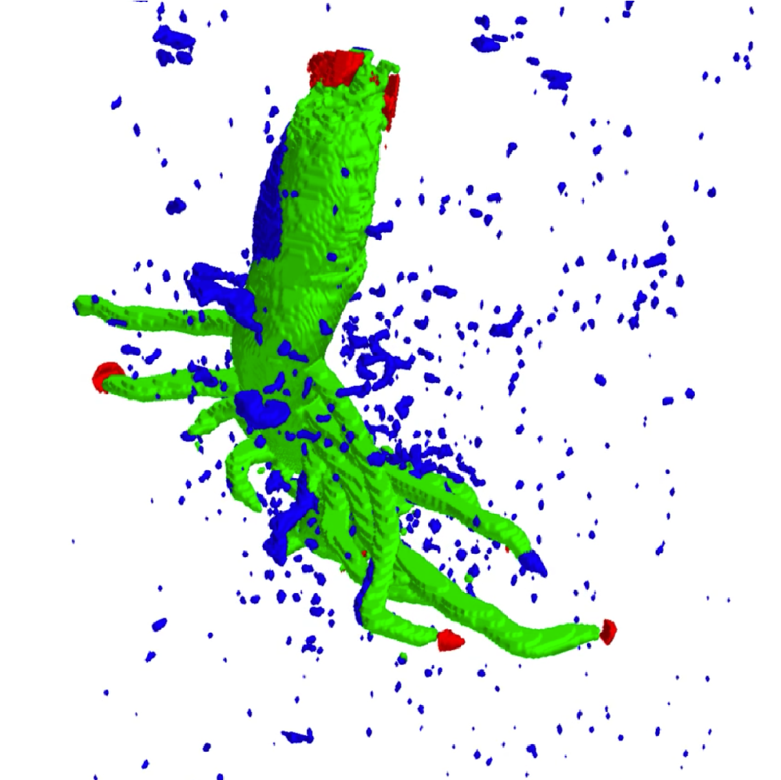 

Root 2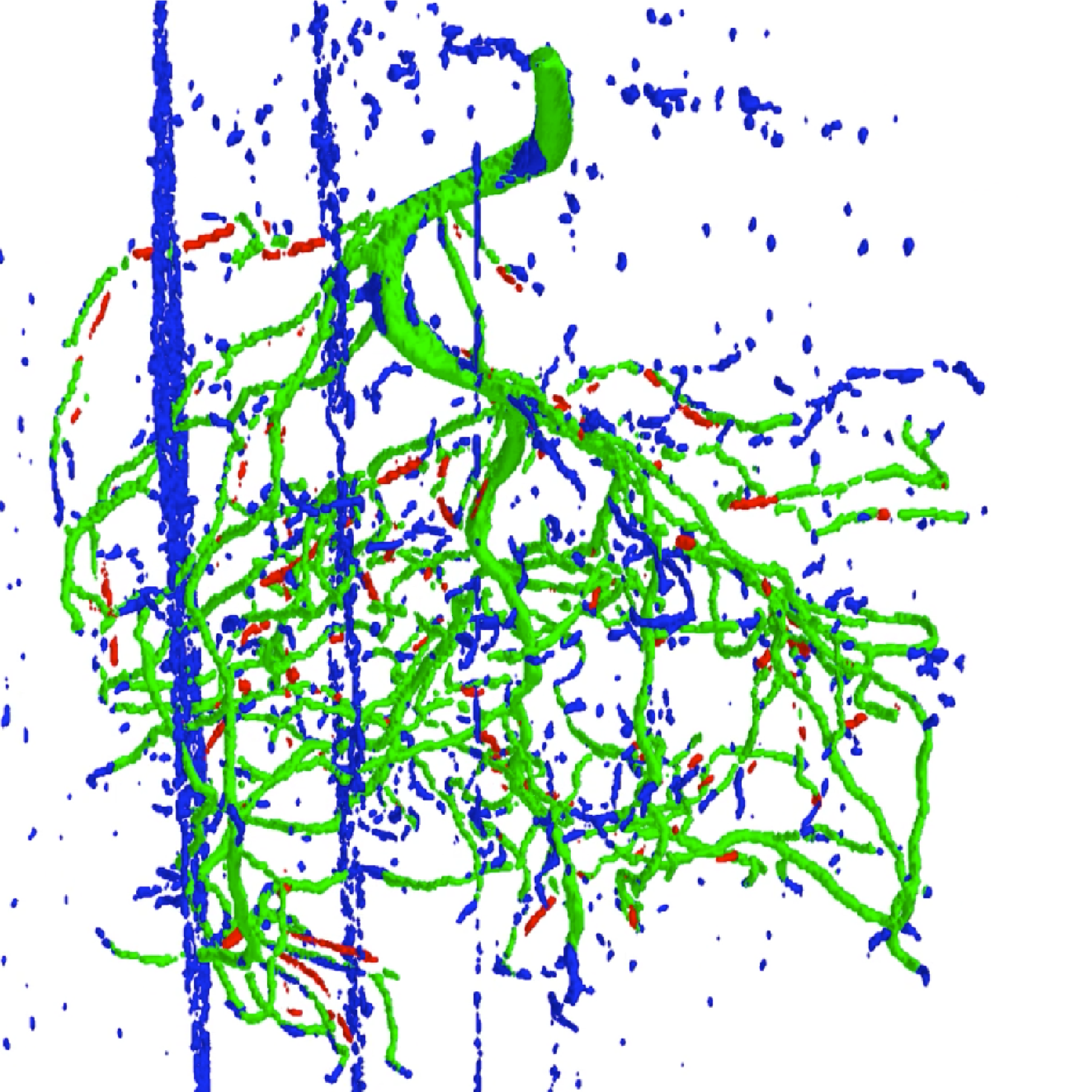 

Figure 4: Performance on real MRI. The bottom row shows segmentations with distance tolerance of 5 voxels (best viewed in color). Green, red and blue represent true positives, false negatives, and false positives, respectively. Root 1 contains minor false positives and almost no false negatives. Root 2 contains minor disconnectivities and MRI artifacts as false positive.

5 Conclusion

We developed a 2D CNN for 3D segmentation of plant root MRI images in super-resolution. As the data we were provided with was too small to train a neural network, we used a transfer learning architecture and generated synthetic training data. With the exception of some extreme cases where the roots are extremely thin, our network performs well on the augmented data. On real data, we successfully detect most of the root structures; including some that are missing in the manual annotations. MRI artifacts introduce false positives in our predictions, which could be mitigated by including these in data augmentation. In future work, the utility of root-thickness dependent losses, data from different growth stages, and additional MRI channels might be investigated.

References

- [1] Dagmar Dusschoten, Ralf Metzner, Johannes Kochs, Johannes A Postma, Daniel Pflugfelder, Jonas Bühler, Ulrich Schurr and Siegfried Jahnke “Quantitative 3D Analysis of Plant Roots growing in Soil using Magnetic Resonance Imaging” In Plant Physiology 170.3 Am Soc Plant Biol, 2016, pp. 1176–1188
- [2] Hannes Schulz, Johannes A Postma, Dagmar Van Dusschoten, Hanno Scharr, Sven Behnke, G Csurka and J Braz “3D Reconstruction of Plant Roots from MRI Images” In Proc. of the International Conference on Computer Vision Theory and Applications (VISAPP), 2012
- [3] Laura Stingaciu, Hannes Schulz, Andreas Pohlmeier, Sven Behnke, Herwig Zilken, Mathieu Javaux and Harry Vereecken “In situ root system architecture extraction from magnetic resonance imaging for water uptake modeling” In Vadose Zone Journal 12.1, 2013
- [4] Kaiming He, Xiangyu Zhang, Shaoqing Ren and Jian Sun “Deep Residual Learning for Image Recognition” In Computer Vision and Pattern Recognition (CVPR), 2016
- [5] J. Carreira and A. Zisserman “Quo Vadis, Action Recognition? A New Model and the Kinetics Dataset” In ArXiv e-prints, 2017 arXiv:1705.07750
- [6] Guosheng Lin, Anton Milan, Chunhua Shen and Ian D Reid “RefineNet: Multi-path Refinement Networks for High-Resolution Semantic Segmentation.” In CVPR, 2017
- [7] L.-C. Chen, G. Papandreou, F. Schroff and H. Adam “Rethinking Atrous Convolution for Semantic Image Segmentation” In ArXiv e-prints, 2017 arXiv:1706.05587
- [8] Jens Kleesiek, Gregor Urban, Alexander Hubert, Daniel Schwarz, Klaus Maier-Hein, Martin Bendszus and Armin Biller “Deep MRI brain extraction: a 3D convolutional neural network for skull stripping” In NeuroImage 129 Elsevier, 2016, pp. 460–469
- [9] Sérgio Pereira, Adriano Pinto, Victor Alves and Carlos A Silva “Brain tumor segmentation using convolutional neural networks in MRI images” In IEEE Tr. on Medical Imaging,, 2016
- [10] Chi-Hieu Pham, Aurélien Ducournau, Ronan Fablet and François Rousseau “Brain MRI super-resolution using deep 3D convolutional networks” In Int. Symp. on Biomedical Imaging, 2017
- [11] Christian Ledig, Lucas Theis, Ferenc Huszár, Jose Caballero, Andrew Cunningham, Alejandro Acosta, Andrew P Aitken, Alykhan Tejani, Johannes Totz, Zehan Wang and Wenzei Shi “Photo-Realistic Single Image Super-Resolution Using a Generative Adversarial Network.” In CVPR, 2017
- [12] Sven Behnke “Learning Iterative Image Reconstruction in the Neural Abstraction Pyramid” In International Journal of Computational Intelligence and Applications World Scientific, 2001
- [13] Jannis Horn “Superresolution 3D Image Segmentation for Plant Root MRI”, 2018
- [14] Jason Yosinski, Jeff Clune, Yoshua Bengio and Hod Lipson “How transferable are features in deep neural networks?” In Advances in Neural Information Processing Systems,, 2014