Calibration of Asynchronous Camera Networks: CALICO

Abstract

Camera network and multi-camera calibration for external parameters is a necessary step for a variety of contexts in computer vision and robotics, ranging from three-dimensional reconstruction to human activity tracking. This paper describes CALICO, a method for camera network and/or multi-camera calibration suitable for challenging contexts: the cameras may not share a common field of view and the network may be asynchronous. The calibration object required is one or more rigidly attached planar calibration patterns, which are distinguishable from one another, such as aruco or charuco patterns.

We formulate the camera network and/or multi-camera calibration problem using rigidity constraints, represented as a system of equations, and an approximate solution is found through a two-step process. Simulated and real experiments, including an asynchronous camera network, multicamera system, and rotating imaging system, demonstrate the method in a variety of settings. Median reconstruction accuracy error was less than $0.41$ mm² for all datasets. This method is suitable for novice users to calibrate a camera network, and the modularity of the calibration object also allows for disassembly, shipping, and the use of this method in a variety of large and small spaces.

1 Introduction

Camera network calibration is necessary for a variety of activities, from human activity detection and recognition to reconstruction tasks. Internal parameters can typically be computed by waving a calibration target in front of cameras, and then using Zhang’s algorithm [1] to calibrate individual cameras. However, determining the external parameters, or the relationships between the cameras in the network, may be a more difficult problem as methods for computing these relationships depend strongly on characteristics of the hardware and the arrangement of the cameras. For instance, the cameras’ shared field of view and level of synchronization strongly influence the ease of camera network calibration.

In this work, we describe a method, CALICO, for camera network calibration assuming that the network is asynchronous. Our method uses calibration objects based on planar aruco or charuco patterns [3] and allows significant implementation flexibility. The datasets and code described in this paper are provided at [4] and https://doi.org/10.5281/zenodo.3520866. A datasheet describing the dataset [5] is in the Supplementary Materials 8.

(a) Datasets Net-1, Net-2

(b) Dataset Mult-1

(c) Dataset Mult-2

Figure 1: Best viewed in color. Cameras and patterns for two types of experiments: asynchronous camera network (top), and multicamera system experiments (bottom). In the top figure, there are 12 cameras. The pattern rig is moved within the workspace, and cameras acquire an image for every move. The bottom row shows a multicamera system, in (b) only two cameras are used while in (c) all four cameras are used. In the multicamera system, the multicamera system is moved and the patterns are stationary. CALICO approximately solves the set of constraints resulting from the camera, pattern, and time relationships in such datasets.

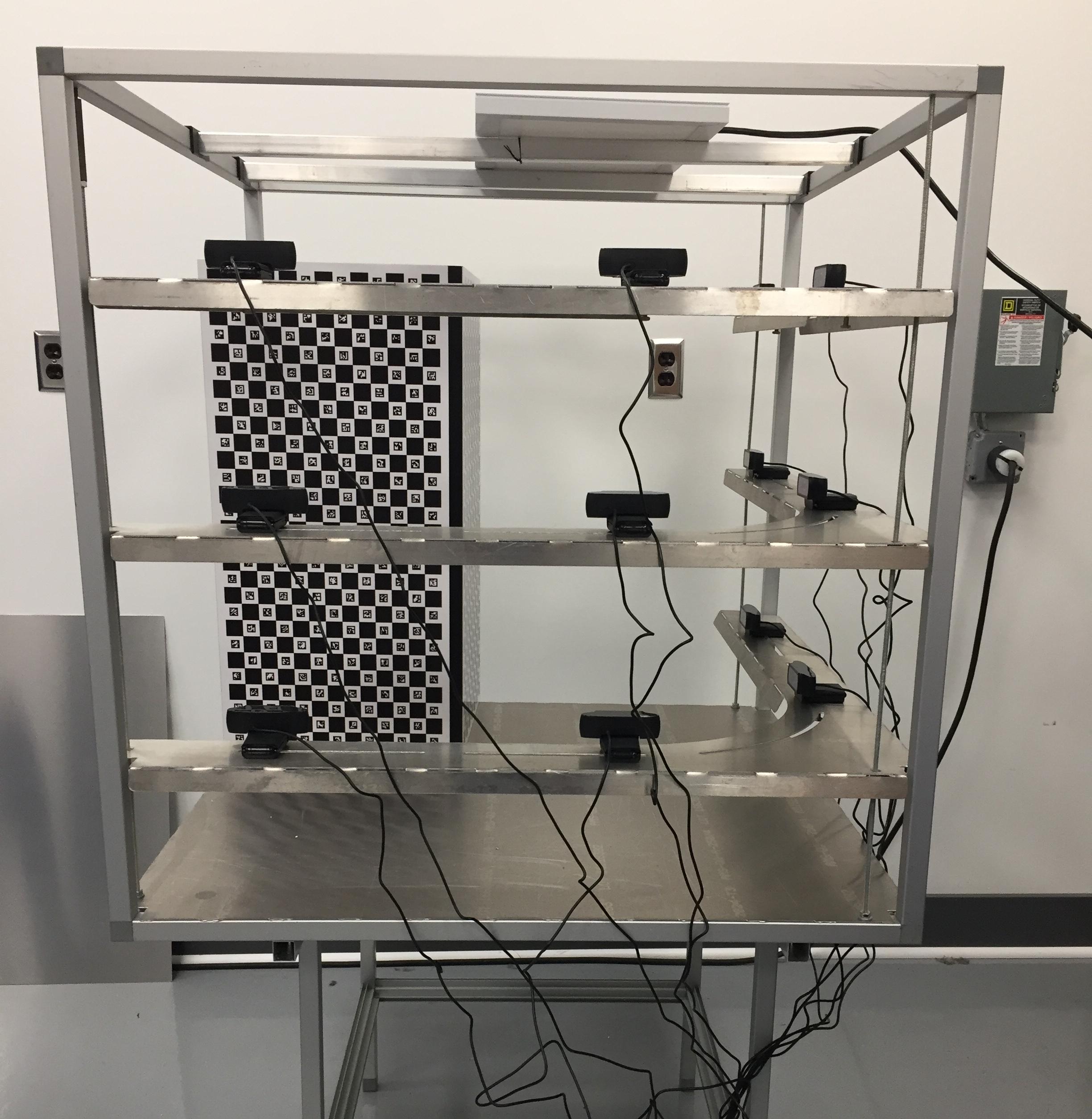
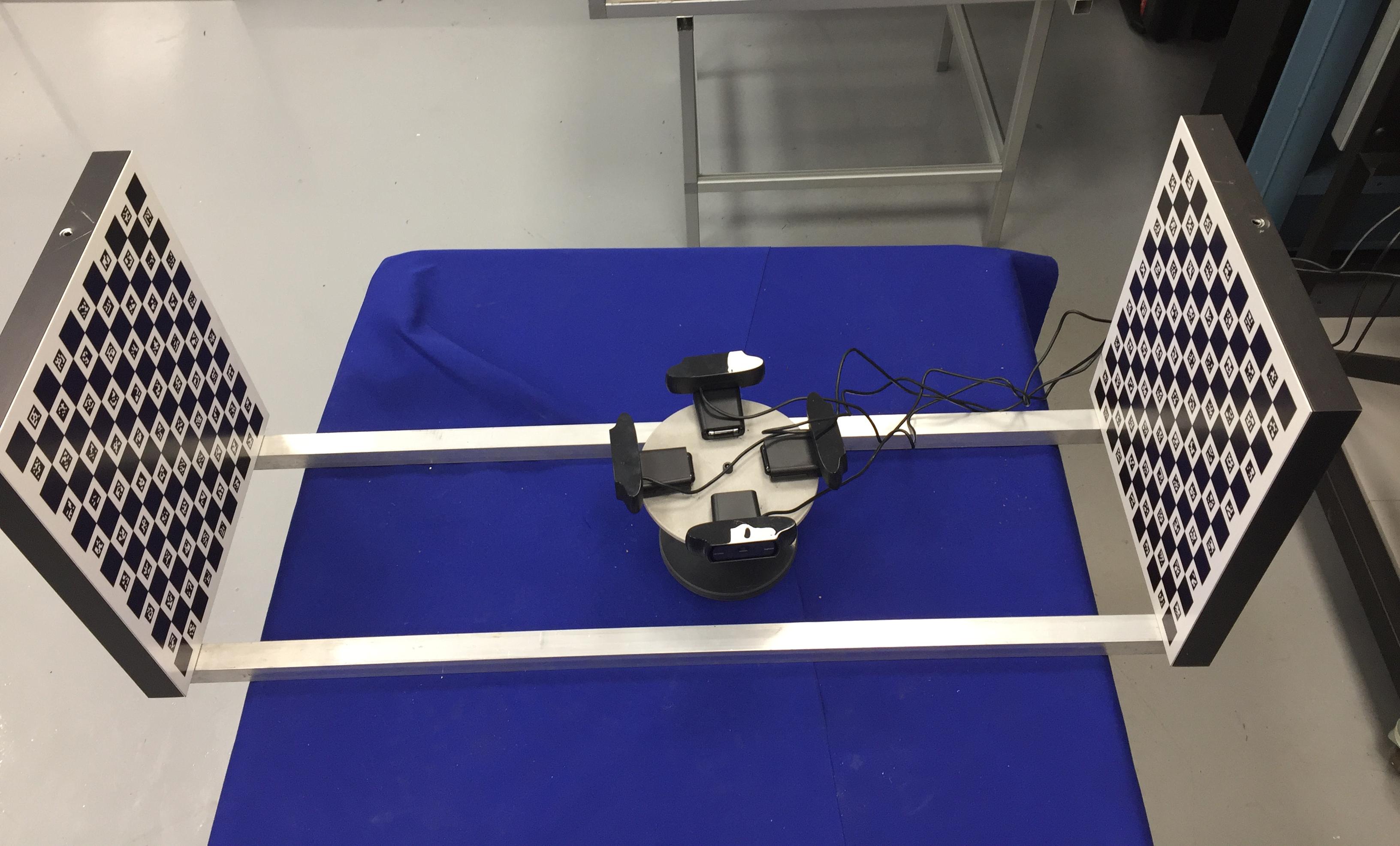
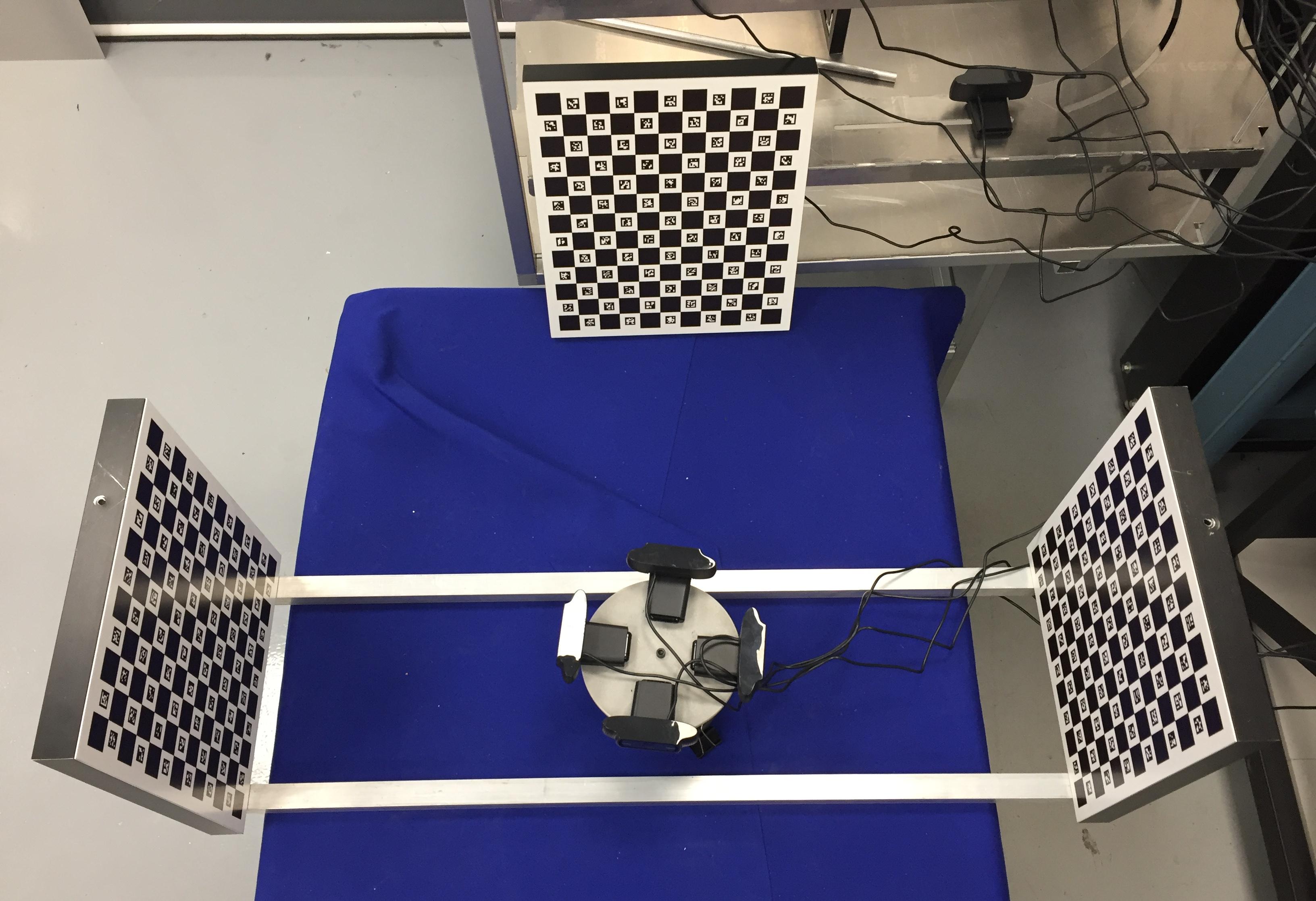
Our motivating application is a low-cost system for densely reconstructing small objects. In multi-view stereo, accurate camera calibration is an important element in the success of such systems [6]. In the context of this work, the objects of interest are from the agricultural domain, reconstructed for plant phenotyping purposes. One of the experiments we use to illustrate this paper consists of a camera network distributed across two sides of a box and pointed generally towards the center, for the reconstruction of small plants. We require that in our future work, camera networks of this type will be constructed, deconstructed, shipped, rebuilt, calibrated, and operated by collaborators in biological laboratories. Consequently, the ultimate aim of this work is a method that allows for the calibration of networks with basic materials, the provision of the code that accompanies the camera-ready version of this paper, and low-cost and interchangeable components.

We will now clarify our use of the ‘camera network’ terminology for camera systems where the camera positions are static. Camera networks usually involve communication between nodes. However, in the literature, multiple-camera systems typically refer to mobile units of cameras, such as stereo heads, or multi-directional clusters of cameras (such as FLIR’s Bumblebee), etc. It is for this reason that we term camera networks those systems that are not mobile, and multicamera systems that are mobile. CALICO may be used in both cases.

Given these preliminaries, our contributions to the state-of-the-art consist of:

1. A method, CALICO, for calibrating camera networks that does not depend on synchronized cameras or common fields of view. CALICO uses images of a simple calibration artifact as input data and can be employed by users without a computer vision background.

2. A formulation of the camera network calibration problem as a set of rigidity constraints imposed by the transformations between cameras, calibration patterns, and movement of the calibration rig, between time instants.

3. The camera network calibration problem is solved efficiently by iteratively solving for variables using closed-form methods, followed by minimization of network-wide reprojection error.

2 Related Work

Camera network calibration: point targets. Synchronized camera networks, such as those used for motion capture and kinematic experiments, have long made use of a protocol of waving a wand, where illuminated LEDs are spaced at known intervals, in front of each camera. These LEDs serve as the world coordinate system. After collecting a large number of images from each camera, structure from motion techniques are used to estimate camera parameters [7, 8, 9, 10].

Multi-camera calibration or asynchronous camera networks. Liu et al. [11] used a two-step approach to calibrate a variety of configurations, including multi-camera contexts, by using robot hand-eye calibration to generate an initial solution, and then minimize reprojection error. The user is required to specify the relationships of camera rig to patterns via a kinematic tree. Joo et al. [12], working with an asynchronous camera network, used patterns projected onto white cloth to calibrate via bundle adjustment.

Robot-camera calibration. The hand-eye calibration problem, and robot-world, hand-eye calibration problem are two formulations of robot-camera calibration using camera and robot pose estimates as data. There has been interest in solving this problem optimally for reconstruction purposes. Tabb and Ahmad Yousef [13, 14] showed that nonlinear minimization of algebraic error, followed by minimization for reprojection error, produced reconstruction-appropriate results for multi-camera, one robot settings. Wei et al. [15] used bundle adjustment to refine initial calibration estimates without a calibration target. Recently, Koide and Menegatti [16] formulated the robot-world, hand-eye calibration problem as a pose-graph optimization problem, which allows for non-pinhole camera models.

CNNs and deep learning. Convolutional neural networks (CNNs) and deep learning have been employed in multiple contexts to predict camera pose. For instance, [17] designed CNNs to predict relative pose in stereo images. Peretroukhin and Kelly [18], in a visual odometry context, use classical geometric and probabilistic approaches, with deep networks used as a corrector [18]. Other works focused on appropriate loss functions for camera pose localization in the context of monocular cameras [19].

Structure from Motion (SfM). CALICO has some similarities with modern SfM pipelines [20, 21] in that local structure is exploited to solve iteratively for cameras; usually this is termed resection. Additionally, there is refinement of the camera pose and scene structure via Levenberg-Marquardt minimization. Since in CALICO the problem is formulated as a set of rigidity constraints, different solving techniques than those used for SfM must be employed.

3 Camera network calibration

The camera network calibration problem consists of determining the relative homogeneous transformation matrices (HTMs) between cameras. First, we will describe the data acquisition design in Section 3.1, which influences the problem formulation for CALICO in Section 3.2.

3.1 Hardware configuration and data acquisition

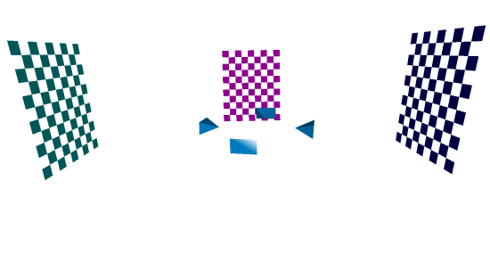
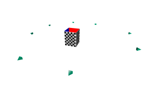
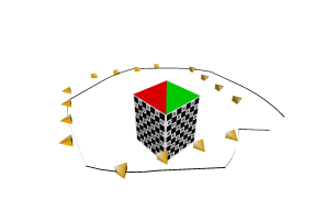
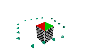
In our implementation, we used a set of two or more planar calibration targets created with chessboard-type aruco tags ([3] and generated with OpenCV [22]), which are referred to as charuco patterns. A four-pattern system, with an eight-camera network, is shown in Figure 2. These patterns are convenient in that we had them printed on aluminum, which can be used outdoors and washed, and their frames can be rigidly attached to one another and then disassembled for shipment. The particular arrangement, and orientation, of the patterns is computed automatically by the algorithm; we refer to the collection of rigidly attached patterns as the calibration rig. As long as a particular calibration pattern’s orientation can be detected, and its pattern index also detected, there is no restriction on the type of pattern used so long as the connections between individual calibration patterns is rigid. For example, one could mount patterns on walls to satisfy the rigidity requirements.

The process of data acquisition is as follows. First, multiple images are acquired per camera to allow for internal parameter calibration, or it is assumed that the cameras are already internally calibrated. Then, the user places the calibration rig in view of at least one camera. Then they indicate that this is time point $t_{0}$ and acquire an image from all cameras. Then, the calibration rig is moved such that at least one or more cameras view a pattern, the user indicates that the current time is time point $t_{1}$ and images are written from all of the cameras. This process is continued until $t_{m}$; minimum specifications on visibility of patterns and cameras and $t_{m}$ is given in Section 4.2.

Although it is important that the cameras and patterns be stationary during image acquisition at a particular time $t$, the use of ‘time $t_{0}$’ does not imply that the cameras are synchronized, but instead that the images be captured and labeled with the same time tag for the same position of the calibration rig. A mechanism for doing so may be implemented through a user interface that allows the user to indicate that all cameras should acquire images, assign them a common time tag, and report to the user when the capture is concluded.

Once images are captured for all $t_{m}$ time steps, camera calibration for internal parameters is performed for each of the cameras independently. Individual patterns are uniquely identified through aruco or charuco tags [3]; cameras’ extrinsic parameters (rotation and translation) are computed with respect to the coordinate systems defined by the patterns recognized in the images. If two (or more) patterns are recognized in the same image, that camera will have two (or more) extrinsic transformations defined for that time instant, one for each of the patterns recognized.

(a) Left: Sim-1 ground truth, Right: Sim-1 result.

(b) Left: Sim-2 ground truth, Right: Sim-2 result.

Figure 2: Best viewed in color. Sim-1 and Sim-2 datasets. The left side of the subfigures shows the ground truth camera poses represented as pyramids, relative to the four charuco patterns. The left side also shows a track of the camera motion relative to the patterns for one camera. The right side of the subfigures shows the camera pose generated by CALICO.

3.2 Problem Formulation

Given the data acquisition procedure outlined in previous sections, our formulation of the camera network calibration problem involves three categories of HTMs: camera $\mathbf{C}$, pattern $\mathbf{P}$ and time $\mathbf{T}$ transformations.

When camera $c$ observes pattern $p$ at time $t$, the HTM relating the coordinate systems of pattern $p$ to camera $c$ can be computed using conventional extrinsic camera calibration methods. We denote this transformation as the HTM ${}^{c}\mathbf{A}_{p}^{t}$. Each HTM is composed of an orthogonal rotation matrix, a translation vector of three elements, and a row of constant terms:

$${}^{c}\mathbf{A}_{p}^{t}=\begin{bmatrix}[l]\mathbf{R}&\mathbf{t}\\ 0^{T}&1\end{bmatrix}.$$ (1)

Suppose a world coordinate system exists, and the calibration rig has its own coordinate system. Then let ${}^{c}\mathbf{C}$ represent the world to camera transformation for camera $c$, ${}^{p}\mathbf{P}$ represent the calibration rig to pattern transformation $p$, and $\mathbf{T}^{t}$ correspond to the world coordinate system to calibration rig coordinate system transformation at time $t$. There is a foundational relationship (FR) between the unknown HTMs ${}^{c}\mathbf{C}$, ${}^{p}\mathbf{P}$, $\mathbf{T}^{t}$, and the known HTMs ${}^{c}\mathbf{A}_{p}^{t}$.

$${}^{c}\mathbf{C}={}^{c}\mathbf{A}_{p}^{t}{}^{p}\mathbf{P}{}\mathbf{T}^{t}.$$ (2)

Each detection of a calibration pattern results in one FR represented by equation Eq. 2. That is, let $\mathbb{C}=\left\{c_{0},c_{1},\ldots,c_{n}\right\}$ be the set of cameras, $\mathbb{T}_{p,c}$ be the set of time instants when pattern $p$ is observed by camera $c$, and $\mathbb{P}_{t,c}$ be the set of patterns observed by camera $c$ at time $t$. Then, the set of foundational relationships is given by

$$\mathbb{FR}=\left\{\right({}^{c}\mathbf{C},{}^{c}\mathbf{A}_{p}^{t},{}^{p}\mathbf{P},\mathbf{T}^{t}\left)\middle|\forall c\in\mathbb{C},\forall t\in\mathbb{T}_{p,c},\forall p\in\mathbb{P}_{t,c}\right\},$$ (3)

where ${}^{c}\mathbf{A}_{p}^{t}$ is known and the other HTMs ${}^{c}\mathbf{C},{}^{p}\mathbf{P},\mathbf{T}^{t}$ are unknown.

For instance, assume camera $c_{0}$ detects pattern $p_{0}$ at times $t_{0}$ and $t_{1}$, and pattern $p_{1}$ at time $t_{1}$, and camera $c_{1}$ detects pattern $p_{1}$ at time $t_{1}$, the set of foundational relationships is equivalent to the following relationships:

$${}^{0}\mathbf{C}={}^{c_{0}}\mathbf{A}_{p_{0}}^{t_{0}}{}^{p_{0}}\mathbf{P}{}\mathbf{T}^{t_{0}}$$ (4)

$${}^{0}\mathbf{C}={}^{c_{0}}\mathbf{A}_{p_{0}}^{t_{1}}{}^{p_{0}}\mathbf{P}{}\mathbf{T}^{t_{1}}$$ (5)

$${}^{0}\mathbf{C}={}^{c_{0}}\mathbf{A}_{p_{1}}^{t_{1}}{}^{p_{1}}\mathbf{P}{}\mathbf{T}^{t_{1}}$$ (6)

$${}^{1}\mathbf{C}={}^{c_{1}}\mathbf{A}_{p_{1}}^{t_{1}}{}{{}^{p_{1}}\mathbf{P}}{}\mathbf{T}^{t_{1}}$$ (7)

Each element of $\mathbb{FR}$ corresponds to one observation for the estimation of the unknown HTMs. We describe the estimation process in Section 4.

The world coordinate system is defined by the coordinate system of a reference pattern $p^{*}$ observed at a reference time $t^{*}$. Hence, ${}^{p^{*}}\mathbf{P}=\mathbf{I}_{4}$ and $\mathbf{T}^{t^{*}}=\mathbf{I}_{4}$, where $\mathbf{I}_{4}$ is an identity matrix of size four. We specify how $p^{*}$ and $t^{*}$ are chosen in Section 4.3. A graphical representation of a foundational relationship is shown in Figure 3.

Figure 3: Graphical representation of the foundational relationship.

4 Estimation of the unknown transformations

Our method to find the unknown transformations consists of five steps, which are summarized in Alg. 1. Each step is described in detail below.

Algorithm 1 CALICO: Camera network calibration algorithm.

1:Set of foundational relationships $\mathbb{FR}$.

2:Set of solutions $\mathbb{V}=\{({}^{c}\mathbf{C},{}^{p}\mathbf{P},\mathbf{T}^{t})|\forall c\in\mathbb{C},\forall t\in\mathbb{T}_{p,c},\forall p\in\mathbb{P}_{t,c}\}$.

3:Determine intrinsic and extrinsic camera parameters with respect to visible patterns at all time instants, 4.1.

4:Verify that the network can be calibrated using FR connectivity test, 4.2.

5:Choose reference pattern $p^{*}$ and time $t^{*}$ and substitute the corresponding HTMs in the set $\mathbb{FR}$ where they appear, 4.3.

6:Find the initial solution set $\mathbb{V}_{0}$ by iteratively solving first individual, and then pairwise uninitialized variables found at prior iterations, 4.4.

7:Find the final solution set $\mathbb{V}$ by refining the estimated HTMs through reprojection error minimization, 4.5.

4.1 Step 1: Intrinsic calibration of individual cameras

Step 1 is a standard component of camera calibration procedures: calibrate cameras for intrinsic and extrinsic camera calibration parameters. Each pattern detection triggers the generation of one FR in Eq. 3. Note that some images may detect more than one pattern for one time instant. Suppose two patterns are detected in one image. Then two FR’s will be generated. We use OpenCV’s implementation of Zhang’s calibration algorithm [22, 1] for this step.

4.2 Step 2: Calibration condition test

To determine if the camera network can be calibrated, we construct an interaction graph of the variables and compute the number of connected components. If there is one connected component, the entire camera network can be calibrated with CALICO.

The nodes of the interaction graph are the variables $\{\mathbb{C}\cup\mathbb{T}_{p,c}\cup\mathbb{P}_{t,c}\}$. Walk through the set $\mathbb{FR}$. For each FR, create an edge between the variables in that FR. Figure 4 illustrate an interaction graph for a small dataset.

If the interaction graph consists of a single connected component, then the entire network may be calibrated with CALICO. If the graph consists of multiple connected components, then the cameras corresponding to each component can be calibrated with respect to each other in the connected component but not with respect to the cameras in a different connected component.

Figure 4: The interaction graph for Dataset Mult-1. Edges connected to Camera ${}^{0}\mathbf{C}$ are blue, those connected to Camera ${}^{1}\mathbf{C}$ are grey. $\mathbf{T}^{0}=t^{*}$ and ${}^{0}\mathbf{P}=p^{*}$ in this dataset.

4.3 Step 3: Reference pattern and time selection

The reference pattern and time are chosen such that the greatest numbers of variables can be initialized. From the list of foundational relationships, the time and pattern combination with the greatest frequency is chosen as the reference pair. That is, the reference pattern is given by

$$p^{*}=\underset{p}{\arg\max}\sum_{c}\left|\mathbb{T}_{p,c}\right|,$$ (8)

which corresponds to the pattern that has been observed the most times by all the cameras. The reference time is given by

$$t^{*}=\underset{t\in\mathbb{T}_{p^{*},c}}{\arg\max}\sum_{c}\left|\mathbb{P}_{t,c}\right|,$$ (9)

which is the time corresponding to the highest number of observations of pattern $p^{*}$. This reference pair is substituted into the list of foundational relationships, ${}^{p^{*}}\mathbf{P}=\mathbf{I}_{4}$ and $\mathbf{T}^{t^{*}}=\mathbf{I}_{4}$.

4.4 Step 4: Initial solution computation

We initialize the set of approximate solutions $\mathbb{V}_{0}=\{({}^{c}\mathbf{C},{}^{p}\mathbf{P},\mathbf{T}^{t})|\forall c\in\mathbb{C},\forall t\in\mathbb{T}_{p,c},\forall p\in\mathbb{P}_{t,c}\}$ by identifying all the elements of $\mathbb{FR}$ for which $p=p^{*}$ and $t=t^{*}$ and computing the corresponding HTM ${}^{c}\mathbf{C}$ for all the cameras that observe the reference pair. At this stage, $|\mathbb{V}_{0}|\geq 3$ since at least one camera transformation can be determined from the reference pair with frequency at least one, and ${}^{p^{*}}\mathbf{P}$, $\mathbf{T}^{t^{*}}\in\mathbb{V}_{0}$.

The solutions in $\mathbb{V}_{0}$ are then substituted into the corresponding elements of $\mathbb{FR}$, and the elements of $\mathbb{FR}$ for which all the variables have initial values are removed from the set. Out of the remaining elements of $\mathbb{FR}$, those with only one unknown variable are then solved and the corresponding solutions are included in $\mathbb{V}_{0}$. If $\mathbb{FR}\neq\emptyset$ and there are no FRs with only one unknown variable, we solve for pairs of variables that interact in elements of $\mathbb{FR}$ using methods for robot-world, hand-eye calibration and add those solutions to the initial solutions set $\mathbb{V}_{0}$. The process of iteratively solving for single or pairs of variables continues until $\mathbb{FR}=\emptyset$.

4.4.1 Solving the relationship equations for a single variable

Let $\mathbb{FR}^{(i)}$ be the set of elements of $\mathbb{FR}$ for which only one HTM variable $\mathbf{X^{(i)}}$ is unknown (at a given iteration, $\mathbf{X}^{(i)}$ could be either ${}^{c}\mathbf{C}$, ${}^{p}\mathbf{P}$, or $\mathbf{T}^{t}$). We solve Eq. 2 for $\mathbf{X}^{(i)}$ by rearranging the terms of the relationship in $\mathbb{FR}^{(i)}$ to the form

$$\mathbf{X^{(i)}}\mathcal{A}=\mathcal{B},,$$ (10)

where $\mathcal{A}$ and $\mathcal{B}$ are the known HTMs and $\mathbf{X^{(i)}}$ is the unknown transformation. If $|\mathbb{FR}^{(i)}|=1$, we simply compute $\mathbf{X^{(i)}}=(\mathcal{A})^{-1}\mathcal{B}$. Otherwise, we combine all the relations in $\mathbb{FR}^{(i)}$ and solve for $\mathbf{X^{(i)}}$ using Shah’s closed-form method for registering two sets of six degree-of-freedom data [23].

4.4.2 Solving the relationship equation for pairs of variables

Similarly, let $\mathbb{FR}^{(i)}$ be the set of elements of $\mathbb{FR}$ for which the HTMs $\mathbf{X^{(i)}}$ and $\mathbf{Z^{(i)}}$ are unknown. We can rearrange Eq. 2, when there are only two unknowns into the form of the robot-world, hand-eye calibration problem

$$\mathcal{A}\mathbf{X^{(i)}}=\mathbf{Z^{(i)}}\mathcal{B},$$ (11)

where $\mathcal{A}$ and $\mathcal{B}$ are known HTMs. We solve for the unknown variables using Shah’s closed-form method for the robot-world, hand-eye problem [24]. Note that $\mathcal{A}$ or $\mathcal{B}$ may be identity matrices in some cases.

4.4.3 Relationship solution order

At each iteration of the process, it may be possible to solve Eq. 3 for more than one transformation. We determine the solution order using a heuristic approach that prioritizes transformations that satisfy the highest number of constraints. That is, we select the HTM $\mathbf{X^{(i)}}$ that maximizes $\left|\mathbb{FR}^{(i)}\right|$. Ties are broken by choosing transformations in the order ${}^{c}\mathbf{C}$, ${}^{p}\mathbf{P}$, $\mathbf{T}^{t}$, and breaking further ties by choosing the transformation with the smallest index first.

We first solve for all of the single variables possible before solving for pairs. Then, we use a similar strategy, that is that ties are broken first with the largest number of $\left|\mathbb{FR}^{(i)}\right|$, and next with the smallest indices.

4.5 Step 5: Reprojection error minimization

Once initial values for all the HTMs are estimated, they are refined by minimizing the reprojection error. Similarly to  [13, 14] in the robot-world, hand-eye calibration problem, the projection matrix ${}^{c}\hat{\mathbf{A}}_{p}^{t}$ can be represented by

$${}^{c}\hat{\mathbf{A}}_{p}^{t}={}^{c}\mathbf{C}\left({\mathbf{T}^{t}}\right)^{-1}{{}^{p}\mathbf{P}}^{-1},$$ (12)

and the relationship between a three-dimensional point $X$ on a calibration pattern and the corresponding two-dimensional point $x$ in the image is

$$x={}^{c}\hat{\mathbf{A}}_{p}^{t}X.$$ (13)

Supposing that the detected image point that corresponds to $X$ is $\tilde{x}$, its reprojection error is $\left\|{x-\tilde{x}}\right\|^{2}$ or, using Eqs. 12 and 13,

$$\left\|{}^{c}\mathbf{C}\left({\mathbf{T}^{t}}\right)^{-1}{{}^{p}\mathbf{P}}^{-1}X-\tilde{x}\right\|{}^{2}.$$ (14)

The total reprojection error is then given by

$$re=\sum_{f\in\mathbb{FR}}\sum_{\left(X,x\right)\in\mathbb{X}_{f}}\left\|{}^{c}\mathbf{C}\left({\mathbf{T}^{t}}\right)^{-1}\left({{}^{p}\mathbf{P}}\right)^{-1}X-{x}\right\|^{2},$$ (15)

where $\mathbb{X}_{f}$ is the set of calibration pattern point pairs $(X,x)$ observed in the computation of the HTM ${}^{c}{A}_{p}^{t}$ corresponding to the FR $f=\left({}^{c}\mathbf{C},{}^{c}\mathbf{A}_{p}^{t},{}^{p}\mathbf{P},\mathbf{T}^{t}\right)\in\mathbb{FR}$.

We minimize Eq. 15 for all the HTMs, except those corresponding to the reference pair $p^{*}$, $t^{*}$, using the Levenberg-Marquardt algorithm. The elements of $\mathbb{V}_{0}$ are used as the initial solution.

4.6 Choosing number of images in real calibration scenarios

While the above sections describe CALICO in very general terms, for calibrating networks in practical scenarios we offer the following details concerning number of images. From Section 4.2, the minimal requirement is that the interaction graph be one connected component, but beyond that, larger values of $t_{m}$ produce better quality initial solutions than smaller values of $t_{m}$. The reason for this, generally, is that the quality of the initial solution (Section 4.4) benefits from additional constraints between variables. The solution quality produced with CALICO can be assessed via the error metrics we will introduce in future sections; if the error is too high, one can acquire more images, add them to the dataset, and recalibrate.

5 Experiments

The method was evaluated in simulated as well as real-world experiments. First, we introduce three evaluation metrics in Section 5.1, and then describe datasets and results in Sections 5.2 and 5.3, respectively. More figures of the results are available in the Supplementary Materials.

We use the implementation of the Levenberg-Marquardt method found in the software package Ceres [25]. The results shown in this paper were generated on a workstation with one 8-core 3.20GHz processor. OpenCV [22] was used to compute the camera calibration parameters.

5.1 Evaluation

We used three metrics to evaluate the accuracy of CALICO: algebraic error, reprojection root mean squared error, and reconstruction accuracy error.

5.1.1 Algebraic error

The algebraic error represents the fit of the estimated HTMs to $\mathbb{FR}$. It is given by

$$ae=\frac{1}{|\mathbb{FR}|}\sum_{f\in\mathbb{FR}}\left\|{}^{c}\mathbf{C}-{}^{c}\mathbf{A}_{p}^{t}{{}^{p}\mathbf{P}}{\mathbf{T}^{t}}\right\|^{2}_{{F}},$$ (16)

where $f=\left({}^{c}\mathbf{C},{}^{c}\mathbf{A}_{p}^{t},{}^{p}\mathbf{P},\mathbf{T}^{t}\right)$ is a FR, and $\left\|\cdot\right\|_{F}$ denotes the Frobenius norm.

5.1.2 The Reprojection Root Mean Squared Error (rrmse)

The reprojection root mean squared error is simply

$$rrmse=\sqrt{\frac{1}{N}re},$$ (17)

where $N=\sum_{f\in\mathbb{FR}}{\left|\mathbb{X}_{f}\right|}$ is the total number of points observed and $re$ is reprojection error from Equation 15.

5.1.3 Reconstruction Accuracy Error

The reconstruction accuracy error, $rae$, is used here in a similar way as in [14], to assess the method’s ability to reconstruct the three-dimensional location of the calibration pattern points. Given detections of a pattern point in images over all cameras and times, the three-dimensional point that generated those pattern points is estimated. The difference between estimated and ground truth world points represents reconstruction accuracy ($rae$). The ground truth consists of the coordinate system defined by the calibration pattern, so it is known even in real settings. A more formal definition follows.

The three-dimensional point $X$ that generated the corresponding image points $x$ can be found by solving the following minimization problem

$$\hat{\mathcal{Y}}=\operatorname*{argmin}\limits_{X}\sum_{f\in\mathbb{FR}}\left\|{}^{c}\mathbf{C}\left({\mathbf{T}^{t}}\right)^{-1}\left({{}^{p}\mathbf{P}}\right)^{-1}X-{x}\right\|^{2}.$$ (18)

$\hat{\mathcal{Y}}$ is found for all calibration pattern points found in two or more FRs, generating the set $\mathbb{Y}$. Then, the reconstruction accuracy error ($rae$) is the squared Euclidean distance between the estimated $\hat{\mathcal{Y}}_{j}$ points and corresponding calibration object points $X_{j}$, where $j$ is the index of $\hat{\mathcal{Y}}$ in set $\mathbb{Y}$. We use the median $rae$ value over the set $\mathbb{Y}$.

$$rae=\operatorname*{median}\limits_{{\mathcal{Y}}_{j}\in\mathbb{Y}}\Big{\{}\left\|\hat{\mathcal{Y}}_{j}-{X}_{j}\right\|^{2}\Big{\}}.$$ (19)

5.2 Datasets

We used four types of datasets: simulated, camera network, multicamera, and a rotating camera setup. They are abbreviated as ‘Sim- ’, ‘Net- ’, ‘Mult- ’, ‘Rot- ’, etc. The datasets are described in terms of numbers of cameras, patterns, and times in Table 1.

Table 1: Description of the datasets.

Dataset	$|\mathbb{FR}|$	cameras	patterns	times ($t_{m}$)
Sim-1	87	8	4	43
Sim-2	472	16	4	37
Net-1	107	12	2	10
Net-2	211	12	2	20
Mult-1	20	2	2	10
Mult-2	20	2	2	10
Mult-3	72	4	3	24
Rot-1	162	1	8	61
Rot-2	163	1	8	62

5.2.1 Simulated experiments

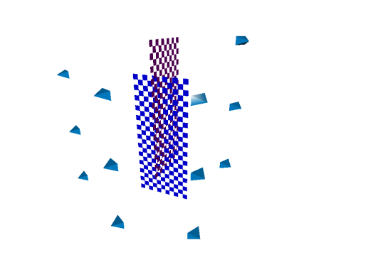
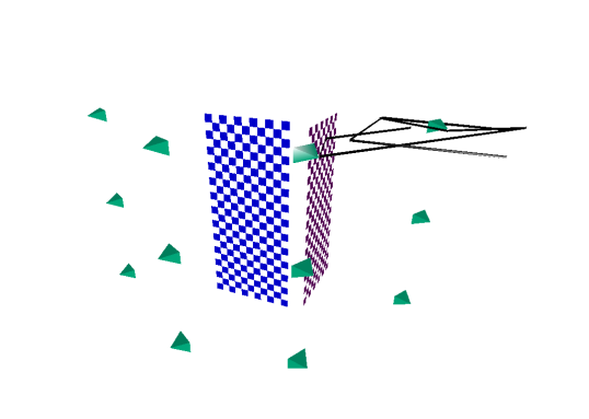
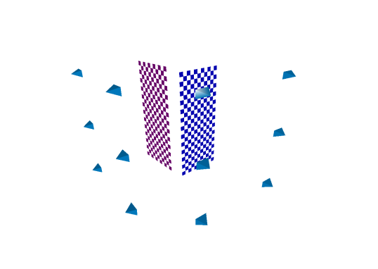
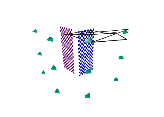
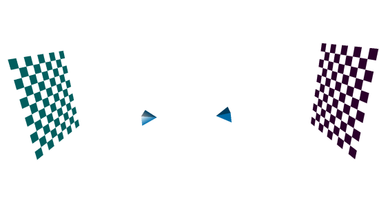
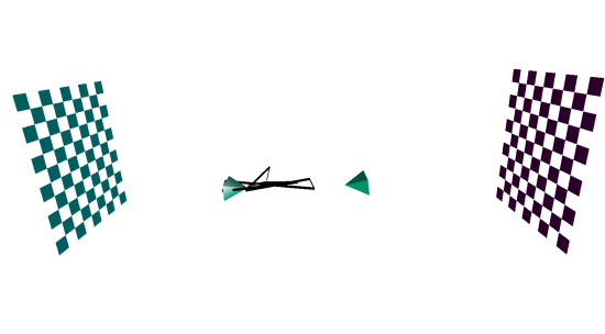
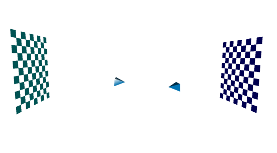
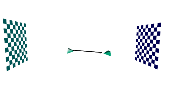
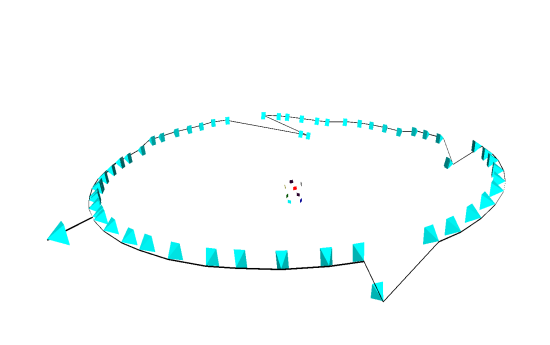
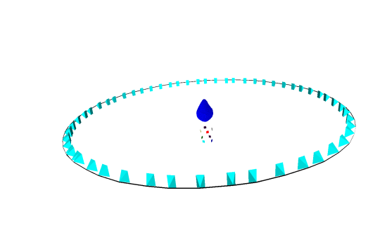
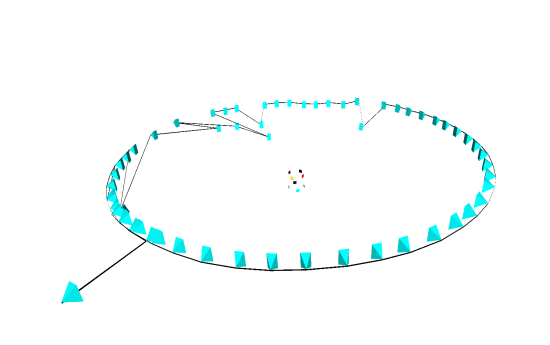
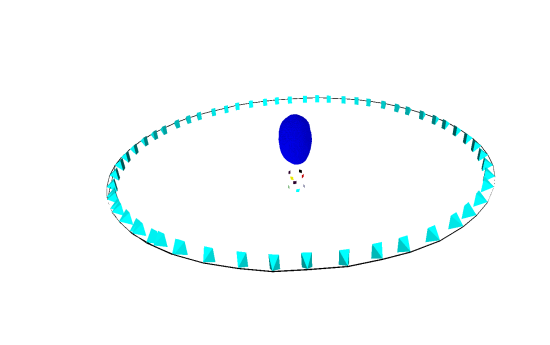
There are two simulated datasets, Sim-1 and Sim-2. OpenGL was used to generate images of charuco patterns from cameras with known parameters. The arrangements of the cameras are shown in Figure 2. Both experiments represent arrangements similar to those used in motion-capture experiments, where cameras are mounted on the wall around a room. They differ in terms of camera density, numbers of cameras, distance from the pattern, and the resulting number of foundational relationships.

5.2.2 Camera network

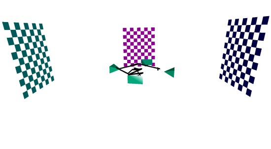
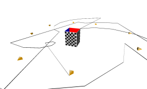
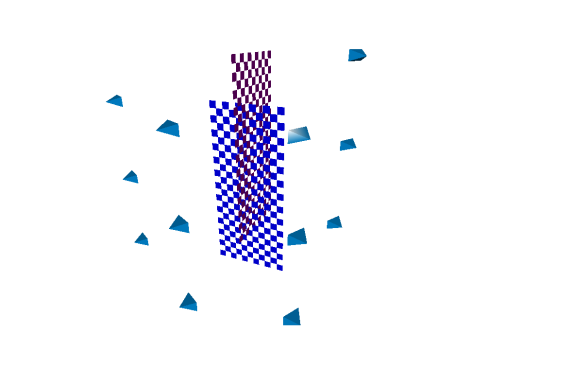
A camera network was constructed using low cost webcameras, and arranged on two sides of a metal rectangular prism, as shown in Figure 1a(a). The calibration rig is constructed of two charuco patterns rigidly attached to each other. To create datasets Net-1 and Net-2, the calibration rig was moved within the workspace. Computed camera positions for Net-1 are shown in Figure 5. Results for Net-2 are shown in the Supplementary Materials.

Figure 5: Best viewed in color. Asynchronous camera network calibration experiment Net-1. Left: initial solution. Right: final solution and track of one camera.

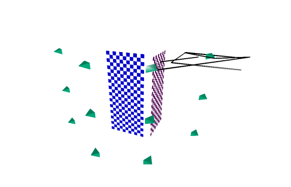
5.2.3 Multicamera rig

Three multicamera datasets were created from four cameras facing away from each other, as in Figure 1b(b-c). In the first two datasets, Mult-1 and Mult-2, only two cameras facing back-to-back from each other were used for data acquisition. In the Mult-1 dataset, each camera in the multicamera rig acquired from only one pattern. In Mult-2, the multicamera rig was rotated half-way through. Doing so created different sets of constraints. Mult-3 uses all four cameras, and uses three calibration patterns. Visualization of the results is shown in the Supplementary Materials.

5.2.4 Rotating object system

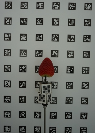
As mentioned previously, the method can be applied to other data acquisition contexts, such as where the goal is to reconstruct an object that is rotating and observed by one camera. In this application, the eventual goal is to phenotype the shape of fruit, such as strawberry.

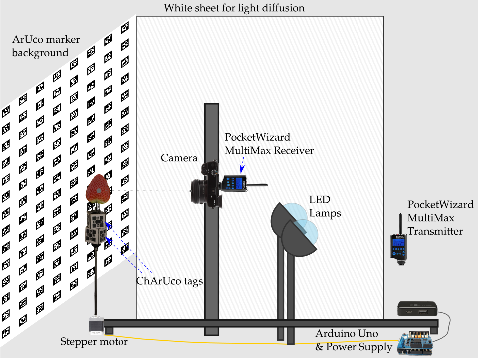
In this experiment, the object was mounted on a spindle. A program triggers the spindle to turn via a stepper motor, as well as to acquire approximately $60$ images from one consumer-grade DSLR camera. On the spindle are two three-dimensional printed cubes, which are rotated from each other by 45 degrees. A charuco pattern is mounted on each visible cube face, totalling $8$ patterns. The experimental setup is shown in the Supplementary Materials and more details available from [26].

CALICO is applied to the rotating experimental design by interpreting each image acquisition of the camera as a time step. The camera is focused between samples, so the background aruco tag image, coupled with exiftag information, is used to calibrate robustly for internal camera parameters.

Following the estimation of the unknown variables for the one camera, eight patterns, and approximately $60$ times, virtual camera positions are generated for each image acquisition relative to the reference pattern and time. In Equation 20, ${}^{0}\mathbf{C}\in\mathbb{V}$ is the HTM representing the sole camera’s pose. For all times $t$, virtual cameras are generated using Eq. 20.

$${{}^{t}\mathbf{C}}={}^{0}\mathbf{C}\left(\mathbf{T}^{t}\right)^{-1}$$ (20)

Results show the distribution of the virtual camera positions over a circle, as expected. Using the method of Tabb [27], the shape of the object is reconstructed. See the Supplementary Materials for these results. Two datasets of this type were used in these experiments, one with strawberry, and another with potato, named Rot-1 and Rot-2.

5.3 Results and discussion

Table 2: Results of using CALICO to compute camera pose for nine datasets. $ae$ has no units, $rrmse$’s units are pixels, median $rae$ is reported, and units are mm². Run time is in seconds.

Dataset	$ae$		$rrmse$		$rae$		run time (s)
	Step 4	Step 5	Step 4	Step 5	Step 4	Step 5
Sim-1	125.221	43.24	15.264	0.428	0.137	0.0188	25.9
Sim-2	791.641	226.52	2.84	0.373	0.190	0.00139	17.9
Net-1	4.559e+06	3.188e+06	428.687	7.603	3.059e+15	0.409	8.9
Net-2	8405.23	9080.08	96.19	0.881	783.56	0.106	12.9
Mult-1	0.363	0.835	3.905	0.406	0.171	0.22	1.6
Mult-2	26.487	3.729	28.173	0.551	1506.67	0.242	1.8
Mult-3	36.494	7.249	20.935	0.725	160.93	0.191	3.4
Rot-1	4550.26	6806.21	140.01	0.256	76.657	0.00188	5.1
Rot-2	4116.67	6241.99	39.137	0.263	4.476	0.00257	6.5

CALICO was used to calibrate the two simulated, two camera network, three multicamera, and two rotating style datasets. Quantitative results are shown in Table 2, and again we refer the reader to the Supplementary Materials for visualizations of the results. Results in terms of the three metrics, algebraic error ($ae$), reprojection root mean squared error ($rrmse$), reconstruction accuracy error ($rae$), and run time. Note that the median $rae$ is more representative than the average, so we report the median in Table 2.

Qualitatively, we found that similarly to SfM, there can be significant drift in the initial solution (Step 4); the quality of this solution depends highly on the poses of the patterns relative to the cameras, and the number of images in the dataset. An example of poor initial solution quality is the Net-1 dataset, where the $ae$ is greater than 1e6 and $rrmse$ is greater than 400. Despite the variety in dataset configurations and numbers of images, CALICO produced camera poses that matched expected positions.

Quantitatively, the camera poses found with CALICO in terms of $rrmse$ were at subpixel values excepting dataset Net-1. The higher $rrmse$ value of that experiment versus the others is perhaps explained by that experiment’s small number of time instants versus a comparably larger number of cameras.

For all of the datasets, CALICO produced a median less than $1$ mm² reconstruction accuracy error, which was surprising. For datasets with many high quality views of the calibration rig, such as the rotating-style datasets, these values are very low ($<0.0026$ mm² or $0.05$ mm).

From Table 2, the algebraic error seems not well related to the quality of results that are important to reconstruction tasks. While algebraic error is used in step 4 to generate initial solutions, algebraic error may be high for views of the calibration patterns where the estimation of the pattern to camera transformation ${}^{c}\mathbf{A}_{p}^{t}$ is not reliable. The rotating-style datasets have a high proportion of images in this category, so we hypothesize that this is why the algebraic error is so high for those datasets.

Minimizing reprojection error, step 5, is the most time-consuming step of the process. Large numbers of foundational relationships also heavily influences run time. Our run time calculations only include the time to compute the camera network calibration portions of the method; in other words, it is assumed that charuco patterns have been detected and cameras calibrated for internal and external parameters (Step 1). Given that, the low run time of CALICO from our experiments is desirable for using this method is a variety of settings.

Application to synchronized camera calibration network. While CALICO was developed for asynchronous networks, it could also be used in synchronized camera network contexts. In these contexts, such as a Vicom or Optitrak systems, the current practice is to wave wand-mounted LEDs in front of each camera. This does not take much time, but calibration data acquisition could be faster by walking through the space with two calibration patterns rigidly attached to each other. Since these systems have an extremely high frame rate, a small subset of images could be chosen to perform the calibration so as not to create an unreasonably large dataset.

6 Conclusions

We presented CALICO, a method for the calibration of asynchronous camera networks, that is suitable for a range of different experimental settings. The performance of the method was demonstrated on nine datasets.

Future work includes incorporating ideas to increase robustness in a range of scenarios. For instance, we wish to explore resection pipelines similar to SfM, where subsets of initial solutions (Step 4) are refined by minimization of reprojection error (Step 5), before solving for more variables.

Other future work includes extending the calibration method to distributed camera networks. For instance, in distributed or asynchronous camera networks, the manual triggering of data acquisition could be automated by monitoring the relative pose between the calibration patterns and the individual cameras at every frame. Once the pose differences stabilize below the expected pose estimation error, the object can be considered stationary, triggering image capture across all the cameras.

7 Supplementary Materials

8 Dataset Datasheet

All of the datasets used in this paper are included in a dataset release at https://doi.org/10.5281/zenodo.3520866 [4]. This section explains the creation of the dataset and other salient details, using the methodology of Gebru et al.2018 [5].

8.1 Motivation for dataset creation

8.1.1 Why was the dataset created?

(e.g., were there specifictasks in mind, or a specific gap that needed to be filled?

8.1.2 What (other) tasks could the dataset be used for?

Arethere obvious tasks for which it shouldnotbe used?Has the dataset been used for any tasks already?If so,where are the results so others can compare (e.g., links topublished papers)?

8.1.3 Who funded the creation of the dataset?

A. Tabb was supported by USDA-ARS National Program 305, Crop Production. M.J. Feldmann’s work is supported in part by grants to Steve J. Knapp from the USDA National Institute of Food and Agriculture Specialty Crops Research Initiative (#2017-51181-26833) and California Strawberry Commission.

8.2 Dataset Composition

8.2.1 What are the instances?

In this collection, there are four types of datasets in general. At the top level, there are two main configurations: network or rotating style data acquisition scenarios. Within that designation, there are two simulated network datasets, and two network datasets from real data. There are three multicamera datasets that fit within the network paradigm, but the cameras move instead of the calibration rig. These are acquired from real data. Finally, there are two rotating-style datasets from real data. The datasets are described in Section 5.2.

8.2.2 Are relationships between instances made explicit in the data?

Yes. Each zipped file represents experiment from the paper and is labeled appropriately.

Image files are .png for all experiments except for ‘Rot-1’ and ‘Rot-2’, where the file format is .JPG. Three-dimensional model files are in .ply format.

8.3 Data collection process

8.3.1 Who was involved in the data collection process?

Amy Tabb collected the data for the ‘Sim-1’, ‘Sim-2’, ‘Net-1’, ‘Net-2’, ‘Mult-1’, ‘Mult-2’, ‘Mult-3’, datasets. Mitchell Feldmann collected the data for the ‘Rot-1’ and ‘Rot-2’ datasets.

8.3.2 Over what time-frame was the data collected?

The ‘Sim-1’, ‘Sim-2’ datasets were collected in September 2019, while ‘Net-1’, ‘Net-2’, ‘Mult-1’, ‘Mult-2’, ‘Mult-3’ were acquired in October 2019. The ‘Rot-1’ and ‘Rot-2’ datasets were acquired in January 2019.

8.3.3 How was the data associated with each instance acquired?

The ‘Sim-1’, ‘Sim-2’ datasets were acquired by a program written in C++ and OpenGL to create a simulated camera network; written by Amy Tabb. The ‘Net-1’, ‘Net-2’, ‘Mult-1’, ‘Mult-2’, ‘Mult-3’ datasets were acquired by a C++ program that acquired images from a network of USB webcameras (Logitech c920 HD Pro Webcameras) using a Gstreamer interface, also written by Amy Tabb. The ‘Rot-1’ and ‘Rot-2’ datasets use a data acquisition environment shown in Figure 8 and described in Feldmann et al.[26]. An Arduino Uno triggers a stepper motor to turn, while a PocketWizard MultiMax Transmitter triggers the camera to acquire images in burst mode and write them to disk. This data acquisition environment was designed by Mitchell Feldmann.

8.3.4 Are there any known errors, sources of noise, or redundancies in the data?

For those datasets with a ground truth, the computation of the projection matrices ${}^{c}\mathbf{A}_{p@t}$ is based on the detection of pattern points in the images. There is less error for the computation of ${}^{c}\mathbf{A}_{p@t}$ when patterns are parallel to the image plane versus perpendicular to it. For this reason, ${}^{c}\mathbf{A}_{p@t}$ contains the types of errors that are common working with real-world imagery. Our intent was compare our method’s performance using the ground truth’s image’s versus the projection matrices from the ground truth.

8.4 Data Preprocessing

8.4.1 What preprocessing/cleaning was done?

No preprocessing was done.

8.5 Data distribution

8.5.1 How is the dataset distributed?

The dataset is stored and distributed via Zenodo. It is available at DOI 10.5281/zenodo.3520866 and has citation [4].

8.5.2 When will the dataset be released/first distributed?

This dataset will first be released in November, 2019.

8.5.3 What license (if any) is it distributed under?

The MIT license is used, and the authors request that at a minimum the corresponding paper be cited.

8.5.4 Are there any fees or access/export restrictions?

There are no fees, but the terms of the MIT license hold, primarily, that the dataset is provided without warranty of any kind.

9 Dataset Maintenance

9.0.1 Who is supporting/hosting/maintaining the dataset?

The dataset is hosted at Zenodo.org and Amy Tabb is maintaining. Comments or requests can be sent to her at amy.tabb@usda.gov.

9.0.2 Will the dataset be updated?

There are not currently plans to update the dataset.

10 Legal and Ethical Considerations

This dataset does contain images of Amy Tabb in the ‘Net-1’ dataset. She is aware and gives her consent to include the data in the dataset.

The maintainers and their institutions are exempt from any liability, judicial or extrajudicial, for any losses or damages arising from the use of the data contained in the image database. The dataset has a the MIT license.

10.1 $\mathbb{FR}$ for Mult-1

Below is the state of the $\mathbb{FR}$ set after step 3. $\mathbf{T}^{0}=t^{*}$ and ${}^{0}\mathbf{P}=p^{*}$, and ${}^{1}\mathbf{C}$ has been initialized.

$${}^{0}\mathbf{C}= {}^{c_{0}}\mathbf{A}_{p_{1}@t_{0}^{*}}{{}^{1}\mathbf{P}}$$ (21)

$${}^{0}\mathbf{C}= {}^{c_{0}}\mathbf{A}_{p_{1}@t_{1}}{{}^{1}\mathbf{P}}{{}^{1}\mathbf{T}}$$ (22)

$${}^{0}\mathbf{C}= {}^{c_{0}}\mathbf{A}_{p_{1}@t_{2}}{{}^{1}\mathbf{P}}{{}^{2}\mathbf{T}}$$ (23)

$${}^{0}\mathbf{C}= {}^{c_{0}}\mathbf{A}_{p_{1}@t_{3}}{{}^{1}\mathbf{P}}{{}^{3}\mathbf{T}}$$ (24)

$${}^{0}\mathbf{C}= {}^{c_{0}}\mathbf{A}_{p_{1}@t_{4}}{{}^{1}\mathbf{P}}{{}^{4}\mathbf{T}}$$ (25)

$${}^{0}\mathbf{C}= {}^{c_{0}}\mathbf{A}_{p_{1}@t_{5}}{{}^{1}\mathbf{P}}{{}^{5}\mathbf{T}}$$ (26)

$${}^{0}\mathbf{C}= {}^{c_{0}}\mathbf{A}_{p_{1}@t_{6}}{{}^{1}\mathbf{P}}{{}^{6}\mathbf{T}}$$ (27)

$${}^{0}\mathbf{C}= {}^{c_{0}}\mathbf{A}_{p_{1}@t_{7}}{{}^{1}\mathbf{P}}{{}^{7}\mathbf{T}}$$ (28)

$${}^{0}\mathbf{C}= {}^{c_{0}}\mathbf{A}_{p_{1}@t_{8}}{{}^{1}\mathbf{P}}{{}^{8}\mathbf{T}}$$ (29)

$${}^{0}\mathbf{C}= {}^{c_{0}}\mathbf{A}_{p_{1}@t_{9}}{{}^{1}\mathbf{P}}{{}^{9}\mathbf{T}}$$ (30)

$${}^{1}\mathds{C}= {}^{c_{1}}\mathbf{A}_{p_{0}^{*}@t_{0}^{*}}$$ (31)

$${}^{1}\mathds{C}= {}^{c_{1}}\mathbf{A}_{p_{0}^{*}@t_{1}}{{}^{1}\mathbf{T}}$$ (32)

$${}^{1}\mathds{C}= {}^{c_{1}}\mathbf{A}_{p_{0}^{*}@t_{2}}{{}^{2}\mathbf{T}}$$ (33)

$${}^{1}\mathds{C}= {}^{c_{1}}\mathbf{A}_{p_{0}^{*}@t_{3}}{{}^{3}\mathbf{T}}$$ (34)

$${}^{1}\mathds{C}= {}^{c_{1}}\mathbf{A}_{p_{0}^{*}@t_{4}}{{}^{4}\mathbf{T}}$$ (35)

$${}^{1}\mathds{C}= {}^{c_{1}}\mathbf{A}_{p_{0}^{*}@t_{5}}{{}^{5}\mathbf{T}}$$ (36)

$${}^{1}\mathds{C}= {}^{c_{1}}\mathbf{A}_{p_{0}^{*}@t_{6}}{{}^{6}\mathbf{T}}$$ (37)

$${}^{1}\mathds{C}= {}^{c_{1}}\mathbf{A}_{p_{0}^{*}@t_{7}}{{}^{7}\mathbf{T}}$$ (38)

$${}^{1}\mathds{C}= {}^{c_{1}}\mathbf{A}_{p_{0}^{*}@t_{8}}{{}^{8}\mathbf{T}}$$ (39)

$${}^{1}\mathds{C}= {}^{c_{1}}\mathbf{A}_{p_{0}^{*}@t_{9}}{{}^{9}\mathbf{T}}$$ (40)

Initialized variables: ${}^{1}\mathbf{C}$ ${{}^{0}\mathbf{P}}$ ${{}^{0}\mathbf{T}}$

Uninitialized variables: ${}^{0}\mathbf{C}$ ${{}^{1}\mathbf{P}}$ ${{}^{1}\mathbf{T}}$ ${{}^{2}\mathbf{T}}$ ${{}^{3}\mathbf{T}}$ ${{}^{4}\mathbf{T}}$ ${{}^{5}\mathbf{T}}$ ${{}^{6}\mathbf{T}}$ ${{}^{7}\mathbf{T}}$ ${{}^{8}\mathbf{T}}$ ${{}^{9}\mathbf{T}}$

10.2 Additional figures

[t]

(a) Net-1

(b) Net-2

Figure 6: Best viewed in color. CALICO results for the asynchronous camera network calibration experiments Net-1, Net-2. Left: Visualization of camera poses and pattern locations for the initial solution; a track for one camera is shown. Right: camera poses and pattern locations for the result, with a track for one camera shown.

(a) Mult-1 results

(b) Mult-2 results

(c) Mult-3 results

Figure 7: Best viewed in color. CALICO results for the multicamera datasets. Left: Visualization of camera poses and pattern locations for the initial solution. Right: camera poses and pattern locations for the result, with a track for one camera shown.

(a) Rot-1, Rot-2 hardware

(b) Raw image

(c) Rot-1 initial solution and result

(d) Rot-2 initial solution and result

Figure 8: Best viewed in color Illustration of a rotating-style data acquisition environment for shape phenotyping of fruit. (a): data acquisition schematic. (b): images from a consumer-model DLSR camera. Aruco patterns in the background are used to aid calibration for internal parameters. (c) and (d), left: Visualization of camera poses and pattern locations for the initial solution; a track for one camera is shown. (c) and (d), right: camera poses and pattern locations for the result, with a track for one camera shown.

References

- [1] Z. Zhang, “A flexible new technique for camera calibration,” Pattern Analysis and Machine Intelligence, IEEE Transactions on, vol. 22, no. 11, pp. 1330–1334, Nov. 2000. [Online]. Available: https://doi.org/10.1109/34.888718
- [2] B. A. Cook, “ACRONYM: Acronym CReatiON for You and Me,” arXiv:1903.12180 [astro-ph], Mar. 2019, arXiv: 1903.12180. [Online]. Available: http://arxiv.org/abs/1903.12180
- [3] S. Garrido-Jurado, R. Muñoz-Salinas, F. Madrid-Cuevas, and M. Marín-Jiménez, “Automatic generation and detection of highly reliable fiducial markers under occlusion,” Pattern Recognition, vol. 47, no. 6, pp. 2280–2292, Jun. 2014. [Online]. Available: https://doi.org/10.1016/j.patcog.2014.01.005
- [4] A. Tabb and M. J. Feldmann, “Data and Code from: Calibration of Asynchronous Camera Networks: CALICO.” Zenodo, Nov. 2019. [Online]. Available: https://doi.org/10.5281/zenodo.3520866
- [5] T. Gebru, J. Morgenstern, B. Vecchione, J. Wortman Vaughan, H. Wallach, H. Daumé III, and K. Crawford, “Datasheets for datasets,” in 5th Workshop on Fairness, Accountability, and Transparency in Machine Learning, Stockholm, Sweden, PMLR 80, 2018., July 2018. [Online]. Available: https://www.microsoft.com/en-us/research/publication/datasheets-for-datasets/
- [6] Y. Furukawa and C. Hernández, “Multi-View Stereo: A Tutorial,” Foundations and Trends® in Computer Graphics and Vision, vol. 9, no. 1-2, pp. 1–148, 2015. [Online]. Available: http://dx.doi.org/10.1561/0600000052
- [7] P. Baker and Y. Aloimonos, “Complete calibration of a multi-camera network.” IEEE Comput. Soc, 2000, pp. 134–141. [Online]. Available: https://doi.org/10.1109/OMNVIS.2000.853820
- [8] N. A. Borghese, P. Cerveri, and P. Rigiroli, “A fast method for calibrating video-based motion analysers using only a rigid bar,” Medical & Biological Engineering & Computing, vol. 39, no. 1, pp. 76–81, Jan. 2001. [Online]. Available: https://doi.org/10.1007/BF02345269
- [9] L. Chiari, U. D. Croce, A. Leardini, and A. Cappozzo, “Human movement analysis using stereophotogrammetry: Part 2: Instrumental errors,” Gait & Posture, vol. 21, no. 2, pp. 197–211, Feb. 2005. [Online]. Available: https://doi.org/10.1016/j.gaitpost.2004.04.004
- [10] R. Summan, S. G. Pierce, C. N. Macleod, G. Dobie, T. Gears, W. Lester, P. Pritchett, and P. Smyth, “Spatial calibration of large volume photogrammetry based metrology systems,” Measurement, vol. 68, pp. 189–200, May 2015. [Online]. Available: https://doi.org/10.1016/j.measurement.2015.02.054
- [11] A. Liu, S. Marschner, and N. Snavely, “Caliber: Camera Localization and Calibration Using Rigidity Constraints,” International Journal of Computer Vision, vol. 118, no. 1, pp. 1–21, May 2016. [Online]. Available: https://doi.org/10.1007/s11263-015-0866-1
- [12] H. Joo, T. Simon, X. Li, H. Liu, L. Tan, L. Gui, S. Banerjee, T. S. Godisart, B. Nabbe, I. Matthews, T. Kanade, S. Nobuhara, and Y. A. Sheikh, “Panoptic Studio: A Massively Multiview System for Social Interaction Capture,” IEEE Transactions on Pattern Analysis and Machine Intelligence, pp. 1–1, 2018. [Online]. Available: http://doi.org/10.1109/TPAMI.2017.2782743
- [13] A. Tabb and K. M. Ahmad Yousef, “Parameterizations for reducing camera reprojection error for robot-world hand-eye calibration,” in 2015 IEEE/RSJ International Conference on Intelligent Robots and Systems (IROS), Sep. 2015, pp. 3030–3037. [Online]. Available: http://doi.org/10.1109/IROS.2015.7353795
- [14] A. Tabb and K. M. Ahmad Yousef, “Solving the robot-world hand-eye(s) calibration problem with iterative methods,” Machine Vision and Applications, vol. 28, no. 5, pp. 569–590, Aug. 2017. [Online]. Available: https://doi.org/10.1007/s00138-017-0841-7
- [15] W. Li, M. Dong, N. Lu, X. Lou, and P. Sun, “Simultaneous robot–world and hand–eye calibration without a calibration object,” Sensors, vol. 18, no. 11, 2018. [Online]. Available: https://doi.org/10.3390/s18113949
- [16] K. Koide and E. Menegatti, “General Hand–Eye Calibration Based on Reprojection Error Minimization,” IEEE Robotics and Automation Letters, vol. 4, no. 2, pp. 1021–1028, Apr. 2019. [Online]. Available: https://doi.org/10.1109/LRA.2019.2893612
- [17] I. Melekhov, J. Ylioinas, J. Kannala, and E. Rahtu, “Relative Camera Pose Estimation Using Convolutional Neural Networks,” in Advanced Concepts for Intelligent Vision Systems, ser. Lecture Notes in Computer Science, J. Blanc-Talon, R. Penne, W. Philips, D. Popescu, and P. Scheunders, Eds. Springer International Publishing, 2017, pp. 675–687. [Online]. Available: https://doi.org/10.1007/978-3-319-70353-4_57
- [18] V. Peretroukhin and J. Kelly, “DPC-Net: Deep Pose Correction for Visual Localization,” IEEE Robotics and Automation Letters, vol. 3, no. 3, pp. 2424–2431, Jul. 2018. [Online]. Available: https://doi.org/10.1109/LRA.2017.2778765
- [19] A. Kendall and R. Cipolla, “Geometric Loss Functions for Camera Pose Regression with Deep Learning,” in 2017 IEEE Conference on Computer Vision and Pattern Recognition (CVPR), Jul. 2017, pp. 6555–6564. [Online]. Available: https://doi.org/10.1109/CVPR.2017.694
- [20] J. L. Schonberger and J.-M. Frahm, “Structure-from-Motion Revisited,” in 2016 IEEE Conference on Computer Vision and Pattern Recognition (CVPR). Las Vegas, NV, USA: IEEE, Jun. 2016, pp. 4104–4113. [Online]. Available: https://doi.org/10.1109/CVPR.2016.445
- [21] N. Snavely, S. M. Seitz, and R. Szeliski, “Photo Tourism: Exploring Photo Collections in 3d,” in ACM SIGGRAPH 2006 Papers, ser. SIGGRAPH ’06. New York, NY, USA: ACM, 2006, pp. 835–846, event-place: Boston, Massachusetts. [Online]. Available: http://doi.acm.org/10.1145/1179352.1141964
- [22] G. Bradski, “The OpenCV Library,” Dr. Dobb’s Journal of Software Tools, 2000.
- [23] M. Shah, “Comparing two sets of corresponding six degree of freedom data,” Computer Vision and Image Understanding, vol. 115, no. 10, pp. 1355–1362, Oct. 2011. [Online]. Available: https://doi.org/10.1016/j.cviu.2011.05.007
- [24] ——, “Solving the Robot-World/Hand-Eye Calibration Problem Using the Kronecker Product,” Journal of Mechanisms and Robotics, vol. 5, no. 3, p. 031007, Jun. 2013. [Online]. Available: https://doi.org/10.1115/1.4024473
- [25] S. Agarwal, K. Mierle, and Others, “Ceres solver,” http://ceres-solver.org.
- [26] M. J. Feldmann, A. Tabb, and S. J. Knapp, “Cost-effective, high-throughput 3d reconstruction method for fruit phenotyping,” in CVPPP 2019: Workshop on Computer Vision Problems in Plant Phenotyping, 2019.
- [27] A. Tabb, “Shape from Silhouette Probability Maps: Reconstruction of Thin Objects in the Presence of Silhouette Extraction and Calibration Error,” in 2013 IEEE Conference on Computer Vision and Pattern Recognition, Jun. 2013, pp. 161–168. [Online]. Available: https://doi.org/10.1109/CVPR.2013.28