A combined first and second order model for a junction with ramp buffer

Jennifer Weißen111University of Mannheim, Department of Mathematics, 68131 Mannheim, Germany (jennifer.weissen@uni-mannheim.de, {kolb,goettlich}@uni-mannheim.de).,   Oliver Kolb11footnotemark: 1,   Simone Göttlich11footnotemark: 1
Abstract

Second order macroscopic traffic flow models are able to reproduce the so-called capacity drop effect, i.e., the phenomenon that the outflow of a congested region is substantially lower than the maximum achievable flow. Within this work, we propose a first order model for a junction with ramp buffer that is solely modified at the intersection so that the capacity drop is captured. Theoretical investigations motivate the new choice of coupling conditions and illustrate the difference to purely first and second order models. The numerical example considering the optimal control of the onramp merging into a main road highlights that the combined model generates similar results as the second order model.

AMS subject classifications: 65M08, 90C30

Keywords: traffic flow, numerical analysis, ramp metering control

1 Introduction

Starting with the pioneering works on the Lighthill-Whitham-Richards (LWR) model [36, 41], traffic flow models based on scalar conservation laws, i.e., macroscopic traffic models, have received considerable attention in the academic literature over the past decades. Macroscopic models are mainly distinguished in first order models, which consist of a scalar conservation law for the traffic density, and second order models, using a system of two conservation or balance laws with an additional equation for the mean traffic speed. The first order LWR model describes the time evolution of the traffic density ρ𝜌\rho. The main drawback of the LWR model is the direct link of the velocity and flux to the traffic density, which does not allow for a correct description of traffic instabilities. Second order models have been developed aiming to improve traffic descriptions. Aw, Rascle and Zhang  [4, 45] introduced the second order ARZ model which is capable to capture traffic instabilities and additionally overcame the drawbacks of earlier developed second order models, see [12]. They introduced a pressure function p(ρ)𝑝𝜌p(\rho) in the dynamics. The pressure function represents an anticipation factor, which takes into account the reaction of drivers to the traffic in front of them [18]. It defines the relation between the density ρ𝜌\rho and the speed v𝑣v in the fundamental diagram via a Lagrangian marker w𝑤w. In comparison to the LWR model, the second order model enables to portray more important traffic phenomena [44]. Greenberg [21] extended the ARZ model with a relaxation term towards a preferred velocity. This extension in turn was further generalized by [42]. Since then, the extension to traffic flow on road networks has been investigated intensively, see for example [7, 10, 23, 28, 29, 17, 19, 20, 31]. The crucial point at intersections is the definition of suitable coupling conditions, i.e., conservation of mass and possibly momentum in the case of second order models.

Many interesting effects within traffic dynamics related to congestion and traffic jams have been investigated for microscopic, mesoscopic and macroscopic traffic models, see [25]. Among these effects, the so-called capacity drop phenomenon is of interest [24, 38, 23, 20, 35]. The capacity drop is the phenomenon that the outflow of a congested region is significantly lower than the maximum achievable flow in this region. A capacity drop is observed when the traffic volume upstream of a bottleneck increases, but the discharge flow leaving the bottleneck decreases in comparison to the flow measured prior to the increase in traffic volume [9]. Studies conducted on freeways showed that the discharge flow diminishes with the onset of upstream queues [22, 5, 8]. This results in a flow lower than the maximum one. The traffic jams arising from the capacity drop at bottlenecks can even become permanent [24].

Specifically, in case of an onramp at a freeway, the capacity drop is explained by the fact that drivers mutually impede each other, when too many vehicles try to access the main road [38]. Additionally, drivers at the incoming road upstream from the onramp entry are impacted and might break and slow down. While vehicles can decelerate fast, the acceleration process takes substantially longer [34].

The capacity drop has major influence on the traffic flow and is especially important in the consideration of traffic control. In general, the observational findings indicate that approaches to control the traffic density are promising for increasing bottleneck discharge flows [9].

Here, we completely stick to the LWR model to describe the dynamics on the roads. To mirror the capacity drop effect, we put special emphasis on the intersections, where the velocities and Lagrangian markers are incorporated to describe the dynamics. The capacity drop is achieved by a flow reduction derived from second order dynamics rather than by an adaption of the fundamental diagram. We therefore consider a first order macroscopic model on the roads and we merely apply adapted coupling conditions of a second order macroscopic model at the junctions. This combination then allows to model the capacity drop effect. A similar approach has been considered in [27], where the LWR model was coupled to a kinetic model at the junctions. Comparable to [27], the combined model is also able to cover the capacity drop phenomenon. As in [13], our model is a first order model with a point constraint at the junction. In both models, the supply function of the outgoing road incorporates information of the upstream traffic conditions. The junction constraint in this work is motivated by the second order ARZ model and combines the first order approach with some second order information. Using the combined model, we apply a discrete optimization approach for the control of the onramp, see e.g. [19, 20, 40]. The combined model serves as a suitable substitute model for a second order model when investigating optimal control strategies for ramp metering.

The paper is organized as follows: In Section 2, we briefly recall the LWR and ARZ model. Section 3.1 discusses the capacity drop. We construct our combined model in Section 3.2 with specific emphasis on the respective demand and supply functions, which determine the flux at the junction. The supply function is analyzed intensively in Section 3.3. In Section 4, we present a numerical comparison for several Riemann problems in the LWR and the combined model based on the discretization in Section 4.1 and Section 4.2. The ability to capture the capacity drop is illustrated in Table 2. Section 4.3 presents a comparison of the combined model with second order models. The numerical discretization for second order models is introduced in Section 4.3.1 and comparisons of the combined model with second order models are drawn in Section 4.3.2. The paper concludes with numerical results for an optimal control problem for ramp metering in Section 4.3.3.

2 Models and notations for traffic flow

We consider a directed graph G=(𝒱,)𝐺𝒱G=(\mathcal{V},\mathcal{E}) with a finite number of roads eE𝑒𝐸e\in E and junctions k𝒱𝑘𝒱k\in\mathcal{V}. The roads e𝑒e are modeled by intervals (ae,be)subscript𝑎𝑒subscript𝑏𝑒(a_{e},b_{e}) with (possibly infinite) lengths Le=beaesubscript𝐿𝑒subscript𝑏𝑒subscript𝑎𝑒L_{e}=b_{e}-a_{e}. Vehicles are treated as a continuum with density ρ𝜌\rho and velocity v𝑣v. We shortly introduce two well-known first and second order macroscopic approaches for traffic flow on networks and explain how they model a junction with ramp buffer.

2.1 The LWR model

Given an initial density ρe(x,0)subscript𝜌𝑒𝑥0\rho_{e}(x,0) and denoting ρe=ρe(x,t)subscript𝜌𝑒subscript𝜌𝑒𝑥𝑡\rho_{e}=\rho_{e}(x,t), the dynamics of the LWR model are given by

tρe+x(ρeV(ρe))=0,(x,t)(ae,be)×0,formulae-sequencesubscript𝑡subscript𝜌𝑒subscript𝑥subscript𝜌𝑒𝑉subscript𝜌𝑒0𝑥𝑡subscript𝑎𝑒subscript𝑏𝑒subscriptabsent0\partial_{t}\rho_{e}+\partial_{x}\left(\rho_{e}V(\rho_{e})\right)=0,\qquad(x,t)\in(a_{e},b_{e})\times\mathbb{R}_{\geq 0}, (1)

on each road e𝑒e. Here, we choose for each road e𝑒e the linear velocity function

V(ρe)=vmax(1ρeρmax),𝑉subscript𝜌𝑒superscript𝑣1subscript𝜌𝑒superscript𝜌V(\rho_{e})=v^{\max}\left(1-\frac{\rho_{e}}{\rho^{\max}}\right), (2)

with maximum velocity vmaxsuperscript𝑣v^{\max} and maximum density ρmaxsuperscript𝜌\rho^{\max} as for example described in [17]. We denote the concave flux function f(ρe)=ρeV(ρe)𝑓subscript𝜌𝑒subscript𝜌𝑒𝑉subscript𝜌𝑒f(\rho_{e})=\rho_{e}V(\rho_{e}). It holds that f(0)=f(ρmax)=0𝑓0𝑓superscript𝜌0f(0)=f(\rho^{\max})=0 and the density ρmax/2superscript𝜌2\nicefrac{{\rho^{\max}}}{{2}} maximizes the flux in the interval [0,ρmax]0superscript𝜌[0,\rho^{\max}]. Traffic flow f𝑓f and velocity V𝑉V are directly coupled to the traffic density ρ𝜌\rho.

Refer to caption

Figure 1: 1-to-1 junction with an onramp

In this work, we are especially interested in the dynamics at a junction with ramp buffer. Figure 1 illustrates the 1-to-1 junction with an onramp at the node ramp, which is examined in the following. For simplicity, we assume as prescribed in (1) that the roads e=1,2𝑒12e=1,2 have the same parameters ρmaxsuperscript𝜌\rho^{\max}, vmaxsuperscript𝑣v^{\max}. At the onramp traffic is allowed to enter the outgoing road e=2𝑒2e=2 and the parameter β𝛽\beta describes the mixture of incoming traffic from road e=1𝑒1e=1 and from the onramp. The quantity l(t)𝑙𝑡l(t) describes the length of the queue at the ramp buffer and is modeled by the following ordinary differential equation (ODE):

dl(t)dt=forin(t)qor(t),t0,formulae-sequenced𝑙𝑡d𝑡superscriptsubscript𝑓orin𝑡subscript𝑞or𝑡𝑡subscriptabsent0\displaystyle\frac{\mathrm{d}l(t)}{\mathrm{d}t}=f_{\operatorname*{or}}^{\operatorname*{in}}(t)-q_{\operatorname*{or}}(t),\qquad t\in\mathbb{R}_{\geq 0}, (3)

where forinsuperscriptsubscript𝑓orinf_{\operatorname*{or}}^{\operatorname*{in}} denotes a (possibly) time–dependent flux that enters the onramp from outside of the network and qorsubscript𝑞orq_{\operatorname*{or}} is the flux that exits from the onramp to the outgoing road e=2𝑒2e=2.

To define an initial value problem for this particular network structure, we consider Riemann data on the incoming and outgoing road, i.e., ρe(x,0)=ρe0subscript𝜌𝑒𝑥0superscriptsubscript𝜌𝑒0\rho_{e}(x,0)=\rho_{e}^{0}, e=1,2𝑒12e=1,2 and a fixed inflow forin>0superscriptsubscript𝑓orin0f_{\operatorname*{or}}^{\operatorname*{in}}>0 from the onramp. The end of the incoming road is set to b1=0subscript𝑏10b_{1}=0 and the beginning of the outgoing road to a2=0subscript𝑎20a_{2}=0, such that the junction is located at x=0𝑥0x=0. Then, the (half-) Riemann problem for the roads and the evolution of the queue length at the junction reads

{tρe+x(ρeV(ρe))=0,(x,t)(ae,be)×0,e=1,2,ρe(x,0)=(ρe+ for x>0ρe for x0.),x(ae,be),e=1,2,dl(t)dt=forinqor(t),t0,l(0)=l0.casessubscript𝑡subscript𝜌𝑒subscript𝑥subscript𝜌𝑒𝑉subscript𝜌𝑒0formulae-sequence𝑥𝑡subscript𝑎𝑒subscript𝑏𝑒subscriptabsent0𝑒12subscript𝜌𝑒𝑥0matrixsuperscriptsubscript𝜌𝑒 for 𝑥0superscriptsubscript𝜌𝑒 for 𝑥0formulae-sequence𝑥subscript𝑎𝑒subscript𝑏𝑒𝑒12d𝑙𝑡d𝑡superscriptsubscript𝑓orinsubscript𝑞or𝑡𝑡subscriptabsent0𝑙0superscript𝑙0otherwise\displaystyle\begin{cases}\partial_{t}\rho_{e}+\partial_{x}\left(\rho_{e}V(\rho_{e})\right)=0,&\qquad(x,t)\in(a_{e},b_{e})\times\mathbb{R}_{\geq 0},~{}e=1,2,\\ \rho_{e}(x,0)=\begin{pmatrix}\rho_{e}^{+}&\mbox{ for }x>0\\ \rho_{e}^{-}&\mbox{ for }x\leq 0.\end{pmatrix},&\qquad x\in(a_{e},b_{e}),~{}e=1,2,\\ \frac{\mathrm{d}l(t)}{\mathrm{d}t}=f_{\operatorname*{or}}^{\operatorname*{in}}-q_{\operatorname*{or}}(t),&\qquad t\in\mathbb{R}_{\geq 0},\\ l(0)=l^{0}.&\end{cases} (4)

Here, l00superscript𝑙00l^{0}\geq 0 indicates the initial buffer load. Depending on whether the road is incoming or outgoing, only one of the Riemann data ρe,ρe+superscriptsubscript𝜌𝑒superscriptsubscript𝜌𝑒\rho_{e}^{-},\rho_{e}^{+} is defined for t=0𝑡0t=0. In particular, for road e=1𝑒1e=1 entering the junction ρ1=ρ10superscriptsubscript𝜌1superscriptsubscript𝜌10\rho_{1}^{-}=\rho_{1}^{0}, and for the road e=2𝑒2e=2 exiting the junction ρ2+=ρ20superscriptsubscript𝜌2superscriptsubscript𝜌20\rho_{2}^{+}=\rho_{2}^{0}. The other datum as well as the flux qor(t)subscript𝑞or𝑡q_{\operatorname*{or}}(t) exiting the onramp is defined by the solution through some suitable coupling conditions at the junction. This will be the focus of this work. We fix a priority parameter β𝛽\beta and define the mixture rule:

(M1)

In case that not all cars can enter the outgoing road, let q𝑞q be the flux that can enter the outgoing road. Then βq𝛽𝑞\beta q comes from the incoming road e=1𝑒1e=1 and (1β)q1𝛽𝑞(1-\beta)q comes from the onramp. In case that the amounts βq𝛽𝑞\beta q (resp. (1β)q1𝛽𝑞(1-\beta)q) cannot be served from the incoming road (resp. onramp), we allow that the missing amount is filled up by the onramp (resp. incoming road).

We define solutions to (4) in the following, compare also [14].

Definition 1.

A triple (ρ1,ρ2,l)subscript𝜌1subscript𝜌2𝑙(\rho_{1},\rho_{2},l) is called an admissible weak solution to (4) if the following holds:

  • The densities ρe:(ae,be)×[0,)[0,ρmax]:subscript𝜌𝑒subscript𝑎𝑒subscript𝑏𝑒00superscript𝜌\rho_{e}\colon(a_{e},b_{e})\times[0,\infty)\rightarrow[0,\rho^{\max}], e=1,2𝑒12e=1,2 are weak solutions such that

    0aebe(ρetϕe+f(ρe)xϕe)dxdt=0,e=1,2,formulae-sequencesuperscriptsubscript0superscriptsubscriptsubscript𝑎𝑒subscript𝑏𝑒subscript𝜌𝑒subscript𝑡subscriptitalic-ϕ𝑒𝑓subscript𝜌𝑒subscript𝑥subscriptitalic-ϕ𝑒differential-d𝑥differential-d𝑡0𝑒12\displaystyle\int_{0}^{\infty}\int_{a_{e}}^{b_{e}}\left(\rho_{e}\partial_{t}\phi_{e}+f(\rho_{e})\partial_{x}\phi_{e}\right)\mathrm{d}x\mathrm{d}t=0,\qquad e=1,2,

    for every test function ϕe:(ae,be)×0:subscriptitalic-ϕ𝑒subscript𝑎𝑒subscript𝑏𝑒subscriptabsent0\phi_{e}:(a_{e},b_{e})\times\mathbb{R}_{\geq 0}\rightarrow\mathbb{R} with compact support.

  • The densities ρesubscript𝜌𝑒\rho_{e}, e=1,2𝑒12e=1,2 satisfy the Kruzhkov entropy condition [32]. I.e., for z𝑧z\in\mathbb{R} and ϕe:(ae,be)×0:subscriptitalic-ϕ𝑒subscript𝑎𝑒subscript𝑏𝑒subscriptabsent0\phi_{e}\colon(a_{e},b_{e})\times\mathbb{R}_{\geq 0}\rightarrow\mathbb{R} smooth, positive with compact support, we have that

    0aebe(|ρez|tϕe+sign(ρez)(f(ρe)f(z))xϕe)dxdt+aebe|ρe0z|ϕe(x,0)dx0,e=1,2.\displaystyle\begin{split}\int_{0}^{\infty}\int_{a_{e}}^{b_{e}}\big{(}\lvert\rho_{e}-z\rvert\partial_{t}\phi_{e}+\operatorname{sign}(\rho_{e}-z)&\left(f(\rho_{e})-f(z)\right)\partial_{x}\phi_{e}\big{)}\mathrm{d}x\mathrm{d}t\\ ~{}&+\int_{a_{e}}^{b_{e}}\lvert\rho_{e}^{0}-z\rvert\phi_{e}(x,0)\mathrm{d}x\geq 0,\qquad e=1,2.\end{split} (5)
  • The Rankine Hugoniot condition at the junction, ensuring conservation of mass, is fulfilled

    f(ρ1(0,t)):=q1+qor(t)=f(ρ2(0,t)):=q2.subscript𝑓subscript𝜌10𝑡assignabsentsubscript𝑞1subscript𝑞or𝑡subscript𝑓subscript𝜌20𝑡assignabsentsubscript𝑞2\displaystyle\underbrace{f\left(\rho_{1}(0,t)\right)}_{:=q_{1}}+q_{\operatorname*{or}}(t)=\underbrace{f\left(\rho_{2}(0,t)\right)}_{:=q_{2}}.
  • The flux entering the outgoing road is maximal subject to the mixture rule (M1).

  • The queue length l𝑙l is a solution of (3) for almost every t0𝑡subscriptabsent0t\in\mathbb{R}_{\geq 0}.

Let q1subscript𝑞1q_{1}, qorsubscript𝑞orq_{\operatorname*{or}} denote the initially unknown mass flux coming from the incoming road and the onramp. The total flux has to exit into the outgoing road such that q2=q1+qorsubscript𝑞2subscript𝑞1subscript𝑞orq_{2}=q_{1}+q_{\operatorname*{or}}. In agreement with the literature [10, 35], we employ the widely used demand and supply formulation for admissible flux values. The fluxes at the junction are bounded by demand and supply

0q1DLWR(ρ1),0qorDor(l),0q2SLWR(ρ2).formulae-sequence0subscript𝑞1superscript𝐷LWRsubscript𝜌10subscript𝑞orsuperscript𝐷or𝑙0subscript𝑞2superscript𝑆LWRsubscript𝜌2\displaystyle 0\leq q_{1}\leq D^{\operatorname*{LWR}}(\rho_{1}),\qquad 0\leq q_{\operatorname*{or}}\leq D^{\operatorname*{or}}(l),\qquad 0\leq q_{2}\leq S^{\operatorname*{LWR}}(\rho_{2}).

These are used to determine the flux at the junction and allow for an appropriate description of the coupling and boundary conditions [35]. The demand DLWR(ρ1)superscript𝐷LWRsubscript𝜌1D^{\operatorname*{LWR}}(\rho_{1}) of the incoming road and the supply SLWR(ρ2)superscript𝑆LWRsubscript𝜌2S^{\operatorname*{LWR}}(\rho_{2}) of the outgoing road are defined as follows:

DLWR(ρ1)={ρ1V(ρ1) if ρ1ρmax2,fmax if ρ1>ρmax2,SLWR(ρ2)={fmax if ρ2ρmax2,ρ2V(ρ2) if ρ2>ρmax2,formulae-sequencesuperscript𝐷LWRsubscript𝜌1casessubscript𝜌1𝑉subscript𝜌1 if subscript𝜌1superscript𝜌2superscript𝑓 if subscript𝜌1superscript𝜌2superscript𝑆LWRsubscript𝜌2casessuperscript𝑓 if subscript𝜌2superscript𝜌2subscript𝜌2𝑉subscript𝜌2 if subscript𝜌2superscript𝜌2\displaystyle D^{\operatorname*{LWR}}(\rho_{1})=\begin{cases}\rho_{1}V(\rho_{1})&\text{ if }\rho_{1}\leq\frac{\rho^{\max}}{2},\\ f^{\max}&\text{ if }\rho_{1}>\frac{\rho^{\max}}{2},\end{cases}\qquad S^{\operatorname*{LWR}}(\rho_{2})=\begin{cases}f^{\max}&\text{ if }\rho_{2}\leq\frac{\rho^{\max}}{2},\\ \rho_{2}V(\rho_{2})&\text{ if }\rho_{2}>\frac{\rho^{\max}}{2},\end{cases} (6)

where fmax=f(ρmax/2)superscript𝑓𝑓superscript𝜌2f^{\max}=f(\nicefrac{{\rho^{\max}}}{{2}}). Moreover, the demand of the onramp is modeled by

Dor(l)={formax if l>0,min{forin(t),formax} otherwise,superscript𝐷or𝑙casessubscriptsuperscript𝑓or if 𝑙0superscriptsubscript𝑓orin𝑡subscriptsuperscript𝑓or otherwise,\displaystyle D^{\operatorname*{or}}(l)=\begin{cases}f^{\max}_{\operatorname*{or}}&\text{ if }l>0,\\ \min\{f_{\operatorname*{or}}^{\operatorname*{in}}(t),f^{\max}_{\operatorname*{or}}\}&\text{ otherwise,}\end{cases} (7)

where formaxsubscriptsuperscript𝑓orf^{\max}_{\operatorname*{or}} denotes the maximum flux which is allowed to enter from the onramp into the outgoing road, i.e., a physical restriction on the number of cars per time unit that can exit from the onramp. Collecting together equations (6)-(7) and the mixture rule (M1), we can formulate the mass fluxes at the 1-to-1 junction with onramp in the compact form

q1subscript𝑞1\displaystyle q_{1} =min{DLWR(ρ1),max{βSLWR(ρ2),SLWR(ρ2)Dor(l)}},absentsuperscript𝐷LWRsubscript𝜌1𝛽superscript𝑆LWRsubscript𝜌2superscript𝑆LWRsubscript𝜌2superscript𝐷or𝑙\displaystyle=\min\{D^{\operatorname*{LWR}}(\rho_{1}),\max\{\beta S^{\operatorname*{LWR}}(\rho_{2}),S^{\operatorname*{LWR}}(\rho_{2})-D^{\operatorname*{or}}(l)\}\},
qorsubscript𝑞or\displaystyle q_{\operatorname*{or}} =min{Dor(l),max{(1β)SLWR(ρ2),SLWR(ρ2)DLWR(ρ1)}},absentsuperscript𝐷or𝑙1𝛽superscript𝑆LWRsubscript𝜌2superscript𝑆LWRsubscript𝜌2superscript𝐷LWRsubscript𝜌1\displaystyle=\min\{D^{\operatorname*{or}}(l),\max\{(1-\beta)S^{\operatorname*{LWR}}(\rho_{2}),S^{\operatorname*{LWR}}(\rho_{2})-D^{\operatorname*{LWR}}(\rho_{1})\}\},
q2subscript𝑞2\displaystyle q_{2} =q1+qor,absentsubscript𝑞1subscript𝑞or\displaystyle=q_{1}+q_{\operatorname*{or}},

see also [19]. The above expression clarifies that the fluxes at the junction are obtained from the densities on incoming and outgoing road as well as the queue length at the onramp. It is a first order approach where velocity and flux at the junction are directly linked to the traffic densities ρ1,ρ2subscript𝜌1subscript𝜌2\rho_{1},\rho_{2}. The demand is obtained purely from the density on the incoming road ρ1subscript𝜌1\rho_{1} and the supply purely from the density on the outgoing road ρ2subscript𝜌2\rho_{2}. All in all, it is a simple and robust model to describe traffic flow [35]. Although the LWR model can predict some traffic situations rather well, the model exhibits various deficits [12]. In general, the model cannot portray traffic instabilities, which include growing traffic waves and so-called capacity drops [44].

2.2 The ARZ and the Greenberg model

In the second order ARZ model, the traffic density ρe=ρe(x,t)subscript𝜌𝑒subscript𝜌𝑒𝑥𝑡\rho_{e}=\rho_{e}(x,t) and velocity ve=ve(x,t)subscript𝑣𝑒subscript𝑣𝑒𝑥𝑡v_{e}=v_{e}(x,t) are not directly coupled, but evolve according to a system of conservation laws

t(ρeρewe)+x(ρeveρevewe)=0,(x,t)(ae,be)×0.formulae-sequencesubscript𝑡subscript𝜌𝑒subscript𝜌𝑒subscript𝑤𝑒subscript𝑥subscript𝜌𝑒subscript𝑣𝑒subscript𝜌𝑒subscript𝑣𝑒subscript𝑤𝑒0𝑥𝑡subscript𝑎𝑒subscript𝑏𝑒subscriptabsent0\partial_{t}\left(\begin{array}[]{c}\rho_{e}\\ \rho_{e}w_{e}\end{array}\right)+\partial_{x}\left(\begin{array}[]{c}\rho_{e}v_{e}\\ \rho_{e}v_{e}w_{e}\end{array}\right)=0,\qquad(x,t)\in(a_{e},b_{e})\times\mathbb{R}_{\geq 0}. (8)

The first equation describes the conservation of mass and the second equation includes the evolution of the vehicle speed. The Lagrangian marker wesubscript𝑤𝑒w_{e} for each road in (8) is defined by the relation

we=ve+p(ρe),subscript𝑤𝑒subscript𝑣𝑒𝑝subscript𝜌𝑒w_{e}=v_{e}+p(\rho_{e}), (9)

where we assume for simplicity that the pressure function p(ρe)𝑝subscript𝜌𝑒p(\rho_{e}) is identical on all roads. The ARZ model is hyperbolic with eigenvalues λ1=veρep(ρe)λ2=vesubscript𝜆1subscript𝑣𝑒subscript𝜌𝑒superscript𝑝subscript𝜌𝑒subscript𝜆2subscript𝑣𝑒\lambda_{1}=v_{e}-\rho_{e}p^{\prime}(\rho_{e})\leq\lambda_{2}=v_{e} and Riemann invariants wesubscript𝑤𝑒w_{e} and vesubscript𝑣𝑒v_{e}, see [4]. In this case, the Lagrangian marker wesubscript𝑤𝑒w_{e} travels with the velocity vesubscript𝑣𝑒v_{e} of the cars. It can be seen as a driver attribute describing the empty road velocity of drivers.

The pressure function p(ρe)ρeγsimilar-to𝑝subscript𝜌𝑒superscriptsubscript𝜌𝑒𝛾p(\rho_{e})\sim\rho_{e}^{\gamma} with γ=2𝛾2\gamma=2 is the prototype function in traffic flow [4, 16] from which the Lagrangian marker (9) is computed. Here, we consider the pressure function from [20, 38, 23] given by

p(ρe)=vmax2(ρeρmax)2,𝑝subscript𝜌𝑒superscript𝑣2superscriptsubscript𝜌𝑒superscript𝜌2p(\rho_{e})=\frac{v^{\max}}{2}\left(\frac{\rho_{e}}{\rho^{\max}}\right)^{2}, (10)

which was derived from microscopic considerations [3]. The pressure function satisfies p(ρe)>0superscript𝑝subscript𝜌𝑒0p^{\prime}(\rho_{e})>0 and ρep′′(ρe)+2p(ρe)>0subscript𝜌𝑒superscript𝑝′′subscript𝜌𝑒2superscript𝑝subscript𝜌𝑒0\rho_{e}p^{\prime\prime}(\rho_{e})+2p^{\prime}(\rho_{e})>0 for all ρesubscript𝜌𝑒\rho_{e}. The former property ensures that the pressure function is strictly increasing and the latter ensures the existence of a point σ(we)𝜎subscript𝑤𝑒\sigma(w_{e}) that maximizes the flux ρeve=ρe(wep(ρe))subscript𝜌𝑒subscript𝑣𝑒subscript𝜌𝑒subscript𝑤𝑒𝑝subscript𝜌𝑒\rho_{e}v_{e}=\rho_{e}(w_{e}-p(\rho_{e})) for a given value of wesubscript𝑤𝑒w_{e}. The inverse function of the pressure function is given by

p1(y)=ρmax(2yvmax)12,superscript𝑝1𝑦superscript𝜌superscript2𝑦superscript𝑣12p^{-1}(y)=\rho^{\max}\left(\frac{2y}{v^{\max}}\right)^{\frac{1}{2}}, (11)

and σ(we)𝜎subscript𝑤𝑒\sigma(w_{e}) can also be computed explicitly

σ(we)=argmaxρe[0,ρmax]ρe(wep(ρe))=ρmax(2we3vmax)12.𝜎subscript𝑤𝑒subscriptargmaxsubscript𝜌𝑒0superscript𝜌subscript𝜌𝑒subscript𝑤𝑒𝑝subscript𝜌𝑒superscript𝜌superscript2subscript𝑤𝑒3superscript𝑣12\sigma(w_{e})=\operatorname*{argmax}_{\rho_{e}\in[0,\rho^{\max}]}\rho_{e}(w_{e}-p(\rho_{e}))=\rho^{\max}\left(\frac{2w_{e}}{3v^{\max}}\right)^{\frac{1}{2}}. (12)

The (half-)Riemann problem for the ARZ model at the 1-to-1 junction with onramp located at x=0𝑥0x=0 reads:

{t(ρeρewe)+x(ρeveρeweve)=0,(x,t)(ae,be)×0e=1,2,(ρe,we)=((ρe+,we+) for x>0(ρe,we) for x0),x(ae,be),e=1,2,dl(t)dt=forinqor(t),t0,l(0)=l0.casessubscript𝑡subscript𝜌𝑒subscript𝜌𝑒subscript𝑤𝑒subscript𝑥subscript𝜌𝑒subscript𝑣𝑒subscript𝜌𝑒subscript𝑤𝑒subscript𝑣𝑒0formulae-sequence𝑥𝑡subscript𝑎𝑒subscript𝑏𝑒subscriptabsent0𝑒12subscript𝜌𝑒subscript𝑤𝑒matrixsuperscriptsubscript𝜌𝑒superscriptsubscript𝑤𝑒 for 𝑥0superscriptsubscript𝜌𝑒superscriptsubscript𝑤𝑒 for 𝑥0formulae-sequence𝑥subscript𝑎𝑒subscript𝑏𝑒𝑒12d𝑙𝑡d𝑡superscriptsubscript𝑓orinsubscript𝑞or𝑡𝑡subscriptabsent0𝑙0superscript𝑙0otherwise\displaystyle\begin{cases}\partial_{t}\left(\begin{array}[]{c}\rho_{e}\\ \rho_{e}w_{e}\end{array}\right)+\partial_{x}\left(\begin{array}[]{c}\rho_{e}v_{e}\\ \rho_{e}w_{e}v_{e}\end{array}\right)=0,&\qquad(x,t)\in(a_{e},b_{e})\times\mathbb{R}_{\geq 0}$,~{}$e=1,2,\\ (\rho_{e},w_{e})=\begin{pmatrix}(\rho_{e}^{+},w_{e}^{+})&\mbox{ for }x>0\\ (\rho_{e}^{-},w_{e}^{-})&\mbox{ for }x\leq 0\end{pmatrix},&\qquad x\in(a_{e},b_{e}),~{}e=1,2,\\ \frac{\mathrm{d}l(t)}{\mathrm{d}t}=f_{\operatorname*{or}}^{\operatorname*{in}}-q_{\operatorname*{or}}(t),&\qquad t\in\mathbb{R}_{\geq 0},\\ l(0)=l^{0}.&\end{cases} (13)

As for the first order model, we formulate the admissible fluxes at the junction through a demand and supply framework. Following [29, 20], the demand and supply functions for the ARZ model are given by

DARZ(ρ,w)={ρ(wp(ρ)) if ρσ(w),σ(w)(wp(σ(w))) if ρ>σ(w),superscript𝐷ARZ𝜌𝑤cases𝜌𝑤𝑝𝜌 if 𝜌𝜎𝑤𝜎𝑤𝑤𝑝𝜎𝑤 if 𝜌𝜎𝑤\displaystyle D^{\operatorname*{ARZ}}(\rho,w)=\begin{cases}\rho(w-p(\rho))&\text{ if }\rho\leq\sigma(w),\\ \sigma(w)(w-p(\sigma(w)))&\text{ if }\rho>\sigma(w),\end{cases} (14)
SARZ(ρ,w)={σ(w)(wp(σ(w))) if ρσ(w),ρ(wp(ρ)) if ρ>σ(w).superscript𝑆ARZ𝜌𝑤cases𝜎𝑤𝑤𝑝𝜎𝑤 if 𝜌𝜎𝑤𝜌𝑤𝑝𝜌 if 𝜌𝜎𝑤\displaystyle S^{\operatorname*{ARZ}}(\rho,w)=\begin{cases}\sigma(w)(w-p(\sigma(w)))&\text{ if }\rho\leq\sigma(w),\\ \rho(w-p(\rho))&\text{ if }\rho>\sigma(w).\end{cases} (15)

Without entering the discussion in detail, by knowledge on the Riemann solution of the hyperbolic second order model, see e.g. [33, 6], we know that the Riemann problem for (8) on the whole line x𝑥x\in\mathbb{R} with traffic state UL=(ρL,ρLwL)subscript𝑈𝐿subscript𝜌𝐿subscript𝜌𝐿subscript𝑤𝐿U_{L}=(\rho_{L},\rho_{L}w_{L}) on the left (x0𝑥0x\leq 0) and UR=(ρR,ρRwR)subscript𝑈𝑅subscript𝜌𝑅subscript𝜌𝑅subscript𝑤𝑅U_{R}=(\rho_{R},\rho_{R}w_{R}) on the right (x>0𝑥0x>0), is solved by a 1-wave connecting UL,U~subscript𝑈𝐿~𝑈U_{L},\tilde{U} and a 2-contact-discontinuity connecting U~,UR~𝑈subscript𝑈𝑅\tilde{U},U_{R}, see also [4]. The intermediate state is given by U~=(ρ~,ρ~wL)~𝑈~𝜌~𝜌subscript𝑤𝐿\tilde{U}=(\tilde{\rho},\tilde{\rho}w_{L}) and satisfies v(U~)=vR𝑣~𝑈subscript𝑣𝑅v(\tilde{U})=v_{R}, i.e., the second order velocity is given by the velocity of the density on the right.

This can be transferred to define solutions to the (half-) Riemann problem in (13). We follow the approach of [20] to define the Riemann solver at the 1-to-1 junction with onramp: We choose to rewrite the supply function (15) at the 1-to-1 junction with onramp depending on the traffic states left and right from the junction

SARZ(ρ1,ρ2,w1,v2)={σ(w1)(w1p(σ(w1))) if ρ~σ(w1),ρ~(w1p(ρ~)) if ρ~>σ(w1).superscript𝑆ARZsubscript𝜌1subscript𝜌2subscript𝑤1subscript𝑣2cases𝜎subscript𝑤1subscript𝑤1𝑝𝜎subscript𝑤1 if ~𝜌𝜎subscript𝑤1~𝜌subscript𝑤1𝑝~𝜌 if ~𝜌𝜎subscript𝑤1S^{\operatorname*{ARZ}}(\rho_{1},\rho_{2},w_{1},v_{2})=\begin{cases}\sigma(w_{1})(w_{1}-p(\sigma(w_{1})))&\text{ if }\tilde{\rho}\leq\sigma(w_{1}),\\ \tilde{\rho}(w_{1}-p(\tilde{\rho}))&\text{ if }\tilde{\rho}>\sigma(w_{1}).\end{cases} (16)

The mass flux at the interface x=0𝑥0x=0 is determined by the intermediate density value ρ~~𝜌\tilde{\rho} where ρ~=ρ~(ρ1,ρ2,w1,v2)~𝜌~𝜌subscript𝜌1subscript𝜌2subscript𝑤1subscript𝑣2\tilde{\rho}=\tilde{\rho}(\rho_{1},\rho_{2},w_{1},v_{2}) is the density of the state U~~𝑈\tilde{U} such that w(U~)=v1+p(ρ1)𝑤~𝑈subscript𝑣1𝑝subscript𝜌1w(\tilde{U})=v_{1}+p(\rho_{1}) and v(U~)=v2𝑣~𝑈subscript𝑣2v(\tilde{U})=v_{2}. By assumption on the pressure function, there exists at most one state with ρ~0~𝜌0\tilde{\rho}\neq 0 satisfying these conditions111We remark that the approach in [20] works with a fixed pressure function p𝑝p. There are also Riemann solvers considering a change in the pressure function after merge type junctions [29, 28]. . The mass fluxes for the 1-to-1 junction with onramp are then given by

q1=min{DARZ(ρ1,w1),max{βSARZ,SARZDor(l)}},qor=min{Dor(l),max{(1β)SARZ,SARZDARZ(ρ1,w1)}},q2=q1+qor,formulae-sequencesubscript𝑞1superscript𝐷ARZsubscript𝜌1subscript𝑤1𝛽superscript𝑆ARZsuperscript𝑆ARZsuperscript𝐷or𝑙formulae-sequencesubscript𝑞orsuperscript𝐷or𝑙1𝛽superscript𝑆ARZsuperscript𝑆ARZsuperscript𝐷ARZsubscript𝜌1subscript𝑤1subscript𝑞2subscript𝑞1subscript𝑞or\displaystyle\begin{split}q_{1}&=\min\bigg{\{}D^{\operatorname*{ARZ}}(\rho_{1},w_{1}),\max\Big{\{}\beta S^{\operatorname*{ARZ}},S^{\operatorname*{ARZ}}-D^{\operatorname*{or}}(l)\Big{\}}\bigg{\}},\\ q_{\operatorname*{or}}&=\min\bigg{\{}D^{\operatorname*{or}}(l),\max\Big{\{}(1-\beta)S^{\operatorname*{ARZ}},S^{\operatorname*{ARZ}}-D^{\operatorname*{ARZ}}(\rho_{1},w_{1})\Big{\}}\bigg{\}},\\ q_{2}&=q_{1}+q_{\operatorname*{or}},\end{split} (17)

where SARZ=SARZ(ρ1,ρ2,w1,v2)superscript𝑆ARZsuperscript𝑆ARZsubscript𝜌1subscript𝜌2subscript𝑤1subscript𝑣2S^{\operatorname*{ARZ}}=S^{\operatorname*{ARZ}}(\rho_{1},\rho_{2},w_{1},v_{2}). One weakness of the ARZ model as pointed out by Greenberg [21] is that drivers travelling at speed vesubscript𝑣𝑒v_{e} in traffic with local density ρesubscript𝜌𝑒\rho_{e} never try to adjust their speed to a maximum allowable speed V(ρe)𝑉subscript𝜌𝑒V(\rho_{e}). The ARZ model was extended by Greenberg [21] with a relaxation term on the right-hand side of the second equation to correct this weakness. Given initial densities and velocities, the traffic dynamics are governed by the equations

t(ρeρewe)+x(ρeveρeweve)=(0ρeveV(ρe)τ),(x,t)(ae,be)×0.formulae-sequencesubscript𝑡subscript𝜌𝑒subscript𝜌𝑒subscript𝑤𝑒subscript𝑥subscript𝜌𝑒subscript𝑣𝑒subscript𝜌𝑒subscript𝑤𝑒subscript𝑣𝑒0subscript𝜌𝑒subscript𝑣𝑒𝑉subscript𝜌𝑒𝜏𝑥𝑡subscript𝑎𝑒subscript𝑏𝑒subscriptabsent0\displaystyle\partial_{t}\left(\begin{array}[]{c}\rho_{e}\\ \rho_{e}w_{e}\end{array}\right)+\partial_{x}\left(\begin{array}[]{c}\rho_{e}v_{e}\\ \rho_{e}w_{e}v_{e}\end{array}\right)=\left(\begin{array}[]{c}0\\ -\rho_{e}\frac{v_{e}-V(\rho_{e})}{\tau}\end{array}\right),\qquad(x,t)\in(a_{e},b_{e})\times\mathbb{R}_{\geq 0}. (24)

The relaxation term on the right-hand side includes that drivers tend to adopt an equilibrium (or preferential) speed V(ρe)𝑉subscript𝜌𝑒V(\rho_{e}). The factor τ>0𝜏0\tau>0 is interpreted as relaxation time towards an equilibrium speed V(ρe)𝑉subscript𝜌𝑒V(\rho_{e}). In the numerical examples, we use the Greenberg model with the LWR velocity given by (2) as equilibrium velocity. The model therefore possibly contains a relaxation towards the LWR model. For τ=𝜏\tau=\infty, we obtain the original ARZ model. For any value τ(0,)𝜏0\tau\in(0,\infty), we obtain the relaxed model to which we will refer to as ”Greenberg model”. The Greenberg model was mathematically derived from car following models in [3]. A generalization with a more flexible source term where the relaxation depends on the density and velocity is considered in [42, 43]. For an analytical convergence analysis of the Greenberg model for τ0𝜏0\tau\rightarrow 0, we refer to [39, 3]. Moreover, some numerical experiments comparing the Greenberg model with the LWR model are discussed in [20].

Remark 1.

The source term in the Greenberg model (24) is relevant for the road dynamics but is neglected when considering Riemann problems at intersections [43]. Coupling conditions for the Greenberg model and the 1-to-1 junction with ramp buffer are therefore also given by (17).

3 Capacity drop and introduction of the combined model

First, we introduce the capacity drop. Then, we establish a new modeling approach, which combines first and second order traffic models at junction points leading to new coupling conditions.

3.1 The capacity drop

Several traffic network models which equip the first order LWR model with coupling conditions at the junction [10, 26, 30] do not reproduce the capacity drop, see also the discussion in [24]. Lebacque [35] introduced an additional new state variable for the junction in the LWR model. Using this modification, the model is able to represent the capacity drop. Haut et al. [24] triggered a capacity drop by considering a g¯¯𝑔\overline{g}-capacity drop function g¯(𝒵)¯𝑔𝒵\overline{g}(\mathcal{Z}) at the junction. If the sum of incoming demands 𝒵𝒵\mathcal{Z} is above the maximum flux fmaxsuperscript𝑓f^{\max} of the outgoing road, the discharge flow at the junction is reduced. The shape of the flow reduction is prescribed by the g¯¯𝑔\overline{g}-capacity drop function. Nonlocal point constraints limiting the discharging flow at the junction by averaging the density conditions upstream are considered in [1]. The constraint function at the junction x=0𝑥0x=0 depends on the solution itself in an upstream neighborhood x<0𝑥0x<0. They analyzed the capacity drop in the model and further extended the nonlocal point constraint to the ARZ model [2].

Within the second order traffic network models, the capacity drop is included more naturally. The junction model by Haut and Bastin [23] is able to reproduce the capacity drop without the introduction of any new parameters compared to those of the single road model (8). Parzani and Buisson [38] study the model from [23] in a traffic scenario where the bottleneck is caused by an onramp. Furthermore, the Riemann solver in [20] for the junction with onramp, which we recalled in Section 2, shows that the Greenberg model is able to portray the capacity drop and can be applied within traffic control strategies.

In general, traffic control strategies aim to reduce the total time drivers spend in a traffic network. Drivers enter highways at onramps on several locations and controlling these entry points by ramp metering approaches can decrease the total travel time in comparison to the uncontrolled case [5]. For example, a control strategy for ramp metering that can manage to sustain high flows at the sources of the network leads to a decrease of the total time spent in the network [37]. A model covering the capacity drop is therefore an essential requirement for the development of traffic control strategies.

3.2 Construction of the combined model

We begin to develop a junction model for the 1-to-1 junction with ramp buffer covering the capacity drop. The junction model (17) of the Greenberg model includes the capacity drop, see [31]. However considering the second order dynamics, it comes at increased computational cost in comparison to the LWR model. The sharp analysis of second order models by Daganzo [12] states that the traffic for low densities is free and similar to the dynamics of the LWR model. We therefore represent the traffic on the incoming and outgoing road by the LWR model, which gives a good description for low densities. Our idea is now to customize the coupling conditions of the LWR model in case of increasing densities upstream of the junction. We denote the new model as augmented LWR model, or shortly ALWR.

By including second order quantities, we seek to achieve a capacity drop similar to the second order models. However, the velocity Ve=V(ρe)subscript𝑉𝑒𝑉subscript𝜌𝑒V_{e}=V(\rho_{e}) stays coupled to the density ρesubscript𝜌𝑒\rho_{e} and the derived w𝑤w-value for each road is always given by w(ρe)=p(ρe)+Ve𝑤subscript𝜌𝑒𝑝subscript𝜌𝑒subscript𝑉𝑒w(\rho_{e})=p(\rho_{e})+V_{e} and thus, also coupled to the density. At the junction point, our coupling conditions do not only consider the actual density ρ2subscript𝜌2\rho_{2}, but additionally the velocity V2subscript𝑉2V_{2} and the upstream w𝑤w-value w1=w(ρ1)subscript𝑤1𝑤subscript𝜌1w_{1}=w(\rho_{1}). The upstream w𝑤w-value induces a nonlocal point constraint, similar to [13] at the junction point, manipulating the flow through the junction such that a capacity drop is achieved. As explained above, our coupling conditions are motivated by the second order coupling conditions for the ARZ model and we combine them with the standard LWR coupling conditions by means of the augmented supply function

SALWR(ρ1,ρ2,l)superscript𝑆ALWRsubscript𝜌1subscript𝜌2𝑙\displaystyle S^{\operatorname*{ALWR}}(\rho_{1},\rho_{2},l) ={SLWR(ρ2)if 0DLWR(ρ1)+Dor(l)fmax,min{SLWR(ρ2),SARZ(ρ1,ρ2,w1,V2)}otherwise.absentcasessuperscript𝑆LWRsubscript𝜌2if 0superscript𝐷LWRsubscript𝜌1superscript𝐷or𝑙superscript𝑓otherwisesuperscript𝑆LWRsubscript𝜌2superscript𝑆ARZsubscript𝜌1subscript𝜌2subscript𝑤1subscript𝑉2otherwise.otherwise\displaystyle=\begin{cases}S^{\operatorname*{LWR}}(\rho_{2})\qquad\text{if }0\leq D^{\operatorname*{LWR}}(\rho_{1})+D^{\operatorname*{or}}(l)\leq f^{\max},\\[2.0pt] \min\{S^{\operatorname*{LWR}}(\rho_{2}),S^{\operatorname*{ARZ}}\left(\rho_{1},\rho_{2},w_{1},V_{2}\right)\}\qquad\text{otherwise.}\end{cases} (25)

To determine the demands, the LWR demand function (6) and the onramp demand (41) is applied. The value 𝒵=DLWR(ρ1)+Dor(l)𝒵superscript𝐷LWRsubscript𝜌1superscript𝐷or𝑙\mathcal{Z}=D^{\operatorname*{LWR}}(\rho_{1})+D^{\operatorname*{or}}(l) indicates the cumulated desired inflow into the outgoing road. It was observed in experiments that the threshold of traffic density at which a capacity drop is observed is merely constant across the observation days [9]. When the demand is at the level of the road capacity, breakdown and congestion occur [38]. Therefore, the exceedance of the road capacity fmaxsuperscript𝑓f^{\max} in (25) is meant to trigger the formation of a jam upstream the junction.

Analogously to [24], the flux value 𝒵𝒵\mathcal{Z} works as a switch that activates a reduction of the flow through the junction. Contrary to their approach, the reduction of the flow here does not only consider the level of the accumulated demand 𝒵𝒵\mathcal{Z}, but also the interplay of (derived) traffic states up- and downstream the junction in SARZsuperscript𝑆ARZS^{\operatorname*{ARZ}} using (16). In comparison with [1], the nonlocality is restricted only to the junction interface x=0𝑥limit-from0x=0-.

In case that the cumulated desired inflow does not exceed the maximum flow fmaxsuperscript𝑓f^{\max} of the outgoing road, the supply function of the LWR model is applied. In contrast, to evaluate the supply at a junction when the desired inflow exceeds the maximum flow, the minimum of the LWR and ARZ supply is used. Meaning that the incoming flow drops below the inflow predicted by the LWR model, if the application of the ARZ model to the situation with derived second order quantity w1subscript𝑤1w_{1} would lead to a lower inflow. In case of a flow reduction in comparison to the LWR model, we determine the flow by the ARZ supply (16) using the derived quantities w1subscript𝑤1w_{1} and V2subscript𝑉2V_{2} in the augmented supply function. For the coupling conditions using the augmented supply function, we introduce a quite useful partition of the phase plane, which we will explain in detail in the following.

3.3 Discussion of the augmented supply function

This section focuses on the investigation of the supply function in the combined model to show that the ALWR model reduces the flux at the junction in case of congestion. We analyze the problem (4) and examine the augmented supply function (25) in case that the desired inflow 𝒵𝒵\mathcal{Z} exceeds the capacity of the outgoing road fmaxsuperscript𝑓f^{\max}.

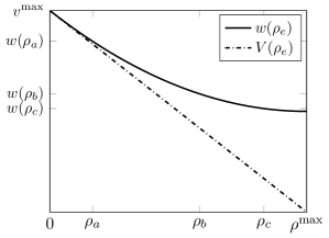
Using the LWR velocity (2) and the pressure function (10), the derived w𝑤w-value reads

w(ρe)=V(ρe)+p(ρe)=vmax(1ρeρmax)+vmax2(ρeρmax)2,𝑤subscript𝜌𝑒𝑉subscript𝜌𝑒𝑝subscript𝜌𝑒superscript𝑣1subscript𝜌𝑒superscript𝜌superscript𝑣2superscriptsubscript𝜌𝑒superscript𝜌2w(\rho_{e})=V(\rho_{e})+p(\rho_{e})=v^{\max}\left(1-\frac{\rho_{e}}{\rho^{\max}}\right)+\frac{v^{\max}}{2}\left(\frac{\rho_{e}}{\rho^{\max}}\right)^{2}, (26)

and is plotted along with the velocity function in Figure 2.
Refer to caption

Figure 2: Derived w𝑤w-values and velocities.

To shorten the notation, we define the derived ARZ supply by

SARZ(ρ1,ρ2)=SARZ(ρ1,ρ2,w1,V2)={σ1(w1p(σ1))if ρ~σ1,ρ~(w1p(ρ~))otherwise,superscript𝑆ARZsubscript𝜌1subscript𝜌2superscript𝑆ARZsubscript𝜌1subscript𝜌2subscript𝑤1subscript𝑉2casessubscript𝜎1subscript𝑤1𝑝subscript𝜎1if ~𝜌subscript𝜎1~𝜌subscript𝑤1𝑝~𝜌otherwise,S^{\operatorname*{ARZ}}(\rho_{1},\rho_{2})=S^{\operatorname*{ARZ}}(\rho_{1},\rho_{2},w_{1},V_{2})=\begin{cases}\sigma_{1}(w_{1}-p(\sigma_{1}))&\text{if }\tilde{\rho}\leq\sigma_{1},\\ \tilde{\rho}(w_{1}-p(\tilde{\rho}))&\text{otherwise,}\end{cases} (27)

in the analysis below. Here, σ1=σ(w1)subscript𝜎1𝜎subscript𝑤1\sigma_{1}=\sigma(w_{1}) is the sonic point given by (12). Note that we are able to do this because we assume that the dynamics on the roads are described by the LWR model.

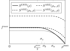
The value w1subscript𝑤1w_{1} scales the supply function and also determines the position of the sonic point σ1subscript𝜎1\sigma_{1}. If we interpret the term (w1p(ρ1))subscript𝑤1𝑝subscript𝜌1(w_{1}-p(\rho_{1})) as the velocity velocity function, then w1subscript𝑤1w_{1} is the empty road velocity. In the ARZ model, w1subscript𝑤1w_{1} is a driver attribute describing the empty road velocity of different drivers and travels with the speed of car. In the LWR model, the empty road velocity is vmaxsuperscript𝑣v^{\max}, which is prescribed by the velocity function (2) and identical for all drivers. Using the derived marker w1subscript𝑤1w_{1} in (27) can be seen as a correction to the empty road velocity depending on the density. For ρ=0𝜌0\rho=0, we obtain w(0)=vmax𝑤0superscript𝑣w(0)=v^{\max}. For ρ=ρmax𝜌superscript𝜌\rho=\rho^{\max}, we obtain w(ρmax)=vmax/2𝑤superscript𝜌superscript𝑣2w(\rho^{\max})=v^{\max}/2 with the specific choices (2) and (10), see also Figure 2. The higher the density, the lower the maximum speed, drivers can reach. Since a reduction in w1subscript𝑤1w_{1} reduces the flux, we can understand the above correction in the w𝑤w-value as a flux reduction for high density values, see Figure 3(a). The value ρ~~𝜌\tilde{\rho} in (27) determines the flux at the junction in the second order model. This intermediate density, which is used to evaluate the supply, is derived from the combination of ρ1subscript𝜌1\rho_{1} and ρ2subscript𝜌2\rho_{2}. Greenberg [21] refers to this property as the anticipatory nature of the ARZ model, i.e., that the density ρ𝜌\rho and velocity v𝑣v behind a contact are also determined by ρ,v𝜌𝑣\rho,v ahead of it. Traditionally, in the coupling at the junction of the LWR model, no connection is made between the states of the incoming and outgoing road in the supply. We therefore introduced ρ~~𝜌\tilde{\rho} motivated from the second order model to combine information from both roads in the supply. Here, the derived value of ρ~~𝜌\tilde{\rho} decides which branch of the supply function (27) is used to evaluate the flux at the junction. It holds that ρ~~𝜌\tilde{\rho} is either the intersection of the curves {w(U)=w1}𝑤𝑈subscript𝑤1\{w(U)=w_{1}\} and {v(U)=V2}𝑣𝑈subscript𝑉2\{v(U)=V_{2}\} or ρ~=0~𝜌0\tilde{\rho}=0, see [4]. We can express ρ~~𝜌\tilde{\rho} explicitly by

ρ~=p1(max{w1V2,0}), where w1=V1+p(ρ1).formulae-sequence~𝜌superscript𝑝1subscript𝑤1subscript𝑉20 where subscript𝑤1subscript𝑉1𝑝subscript𝜌1\tilde{\rho}=p^{-1}(\max\{w_{1}-V_{2},0\}),\qquad\text{ where }w_{1}=V_{1}+p(\rho_{1}). (28)

If we plug ρ~~𝜌\tilde{\rho} in the augmented supply function (25), then the augmented supply can either take the value of the LWR supply or the derived ARZ supply. In situations where the LWR supply is lower than the derived ARZ supply, the ALWR model is equal to the LWR model in its description of traffic dynamics. On the other hand, in situations where the derived ARZ supply is lower than the LWR supply, traffic flow at the junction is reduced and the model differs from the LWR model. Note that we aim to approximate the fluxes at the junction in the ARZ model, but not the traffic state or the solution structure since we keep the LWR model on the roads and only approximate the flux at the junction point.
Refer to caption

(a)

Refer to caption

(b)
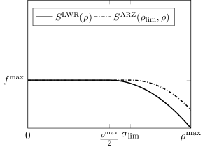
Figure 3: Supply functions.

With ρlimsubscript𝜌lim\rho_{\operatorname*{lim}}, we denote the density for which we have

SARZ(ρlim,0)=fmax,superscript𝑆ARZsubscript𝜌lim0superscript𝑓S^{\operatorname*{ARZ}}(\rho_{\operatorname*{lim}},0)=f^{\max}, (29)

see Figure 3(b). This is used, among other criteria, to distinguish whether the ARZ or LWR supply is applied. The w𝑤w-value is denoted wlim=w(ρlim)subscript𝑤lim𝑤subscript𝜌limw_{\operatorname*{lim}}=w(\rho_{\operatorname*{lim}}). Plugging the densities ρ1subscript𝜌1\rho_{1}, ρ2subscript𝜌2\rho_{2} at the junction into the augmented supply function, we can distinguish the following cases:

Case 1

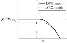
The LWR supply SLWR(ρ2)superscript𝑆LWRsubscript𝜌2S^{\operatorname*{LWR}}(\rho_{2}) exceeds the maximum of the ARZ supply, which is exemplarily depicted in Figure 4(a). The maximum of the ARZ supply (27) is SARZ(ρ1,0)superscript𝑆ARZsubscript𝜌10S^{\operatorname*{ARZ}}(\rho_{1},0) for which ρ~=0~𝜌0\tilde{\rho}=0 since w1vmaxsubscript𝑤1superscript𝑣w_{1}\leq v^{\max}. The exceedance is only possible for ρ1ρlimsubscript𝜌1subscript𝜌lim\rho_{1}\leq\rho_{\operatorname*{lim}}. In this case, the considered supply is the supply value from the ARZ model. This result is independent of the value ρ~~𝜌\tilde{\rho}:

SLWR(ρ2)>SARZ(ρ1,0)min{SLWR(ρ2),SARZ(ρ1,ρ2)}=SARZ(ρ1,ρ2).formulae-sequencesuperscript𝑆LWRsubscript𝜌2superscript𝑆ARZsubscript𝜌10superscript𝑆LWRsubscript𝜌2superscript𝑆ARZsubscript𝜌1subscript𝜌2superscript𝑆ARZsubscript𝜌1subscript𝜌2\displaystyle S^{\operatorname*{LWR}}(\rho_{2})>S^{\operatorname*{ARZ}}(\rho_{1},0)\quad\Rightarrow\qquad\min\{S^{\operatorname*{LWR}}(\rho_{2}),S^{\operatorname*{ARZ}}(\rho_{1},\rho_{2})\}=S^{\operatorname*{ARZ}}(\rho_{1},\rho_{2}).

Refer to caption

(a)

Refer to caption

(b)

Refer to caption

(c)
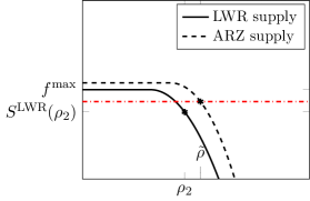
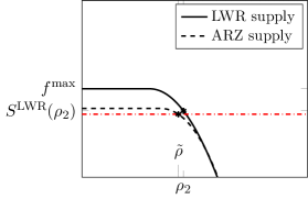
Figure 4: Supply functions. The red line marks the value of SARZsuperscript𝑆ARZS^{\operatorname*{ARZ}}.
Case 2

The LWR supply for ρ2subscript𝜌2\rho_{2} exceeds the ARZ supply for some values, but it is below the maximum of the ARZ supply,

SLWR(ρ2)SARZ(ρ1,0),superscript𝑆LWRsubscript𝜌2superscript𝑆ARZsubscript𝜌10S^{\operatorname*{LWR}}(\rho_{2})\leq S^{\operatorname*{ARZ}}(\rho_{1},0),

Then, one has to distinguish further depending on ρ~~𝜌\tilde{\rho}:

(a)

The ARZ supply evaluated at ρ~~𝜌\tilde{\rho} exceeds the LWR supply at ρ2subscript𝜌2\rho_{2}, see Figure 4(b). The ALWR model uses the same supply function as the LWR model in this case. Therefore, we have

min{SLWR(ρ2),SARZ(ρ1,ρ2)}=SLWR(ρ2).superscript𝑆LWRsubscript𝜌2superscript𝑆ARZsubscript𝜌1subscript𝜌2superscript𝑆LWRsubscript𝜌2\min\{S^{\operatorname*{LWR}}(\rho_{2}),S^{\operatorname*{ARZ}}(\rho_{1},\rho_{2})\}=S^{\operatorname*{LWR}}(\rho_{2}).
(b)

The contrary is true and we have

min{SLWR(ρ2),SARZ(ρ1,ρ2)}=SARZ(ρ1,ρ2).superscript𝑆LWRsubscript𝜌2superscript𝑆ARZsubscript𝜌1subscript𝜌2superscript𝑆ARZsubscript𝜌1subscript𝜌2\min\{S^{\operatorname*{LWR}}(\rho_{2}),S^{\operatorname*{ARZ}}(\rho_{1},\rho_{2})\}=S^{\operatorname*{ARZ}}(\rho_{1},\rho_{2}).

The ALWR model therefore uses the supply function of the ARZ model, see Figure 4(c).

Table 1: Classification of the supply function.
Supply Area
𝒵>fmax𝒵superscript𝑓\mathcal{Z}>f^{\max} ρ1>ρlimsubscript𝜌1subscript𝜌lim\rho_{1}>\rho_{\operatorname*{lim}} ρ2ρmax/2subscript𝜌2superscript𝜌2\rho_{2}\leq\nicefrac{{\rho^{\max}}}{{2}} ARZ I
ρ2>ρmax2subscript𝜌2superscript𝜌2\rho_{2}>\frac{\rho^{\max}}{2} ρ2<σ1subscript𝜌2subscript𝜎1\rho_{2}<\sigma_{1} SARZ(ρ1,0)SLWR(ρ2)superscript𝑆ARZsubscript𝜌10superscript𝑆LWRsubscript𝜌2S^{\operatorname*{ARZ}}(\rho_{1},0)\geq S^{\operatorname*{LWR}}(\rho_{2}) LWR II
SARZ(ρ1,0)<SLWR(ρ2)superscript𝑆ARZsubscript𝜌10superscript𝑆LWRsubscript𝜌2S^{\operatorname*{ARZ}}(\rho_{1},0)<S^{\operatorname*{LWR}}(\rho_{2}) ARZ III
ρ2σ1subscript𝜌2subscript𝜎1\rho_{2}\geq\sigma_{1} ρ1ρ2subscript𝜌1subscript𝜌2\rho_{1}\leq\rho_{2} LWR IV
ρ1>ρ2subscript𝜌1subscript𝜌2\rho_{1}>\rho_{2} SARZ(ρ1,0)SLWR(ρ2)superscript𝑆ARZsubscript𝜌10superscript𝑆LWRsubscript𝜌2S^{\operatorname*{ARZ}}(\rho_{1},0)\geq S^{\operatorname*{LWR}}(\rho_{2}) ARZ V
SARZ(ρ1,0)<SLWR(ρ2)superscript𝑆ARZsubscript𝜌10superscript𝑆LWRsubscript𝜌2S^{\operatorname*{ARZ}}(\rho_{1},0)<S^{\operatorname*{LWR}}(\rho_{2}) ARZ VI
ρ1ρlimsubscript𝜌1subscript𝜌lim\rho_{1}\leq\rho_{\operatorname*{lim}} LWR VII

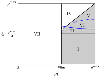
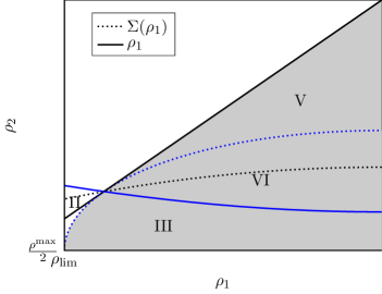
Based on the previous discussion of the augmented supply function, we investigate whether the ARZ supply or the LWR supply is lower for different combinations of initial states (ρ1,ρ2)[0,ρmax]2subscript𝜌1subscript𝜌2superscript0superscript𝜌2(\rho_{1},\rho_{2})\in[0,\rho^{\max}]^{2}. The summarized cases presented in Table 1 lead to a partitioning of the ρ1subscript𝜌1\rho_{1}-ρ2subscript𝜌2\rho_{2}-plane, which is shown in Figure 5. Note that the figure is only valid for 𝒵=Dor+DLWR(ρ1)>fmax𝒵superscript𝐷orsuperscript𝐷LWRsubscript𝜌1superscript𝑓\mathcal{Z}=D^{\operatorname*{or}}+D^{\operatorname*{LWR}}(\rho_{1})>f^{\max}. The ARZ supply is applied in the areas I, III, V and VI while the LWR supply is applied in the areas II, IV and VII.

In the following, we prove this partitioning. Let us start with some notation to ease computations. We denote the maximum of the flux curve associated with the density ρ1subscript𝜌1\rho_{1} by

σ1=σ(w1)=(12)ρmax2w13vmax.subscript𝜎1𝜎subscript𝑤1italic-(12italic-)superscript𝜌2subscript𝑤13superscript𝑣\sigma_{1}=\sigma(w_{1})\overset{\eqref{eq:sonicpoint}}{=}\rho^{\max}\sqrt{\frac{2w_{1}}{3v^{\max}}}. (30)

We have that

σ(ρmax)=13ρmaxσ1σ(0)=23ρmax.𝜎superscript𝜌13superscript𝜌subscript𝜎1𝜎023superscript𝜌\sigma(\rho^{\max})=\sqrt{\frac{1}{3}}\rho^{\max}\leq\sigma_{1}\leq\sigma(0)=\sqrt{\frac{2}{3}}\rho^{\max}.

Plugging the density dependence of w1subscript𝑤1w_{1} given by (26) in (30), we denote the curve of maxima

(ρ1)=(26)ρmax13(ρmaxρ1ρmax)2+13.subscript𝜌1italic-(26italic-)superscript𝜌13superscriptsuperscript𝜌subscript𝜌1superscript𝜌213\mathcal{M}(\rho_{1})\overset{\eqref{calc:functionwofrho}}{=}\rho^{\max}\sqrt{\frac{1}{3}\left(\frac{\rho^{\max}-\rho_{1}}{\rho^{\max}}\right)^{2}+\frac{1}{3}}. (31)

Therefore, the curve (ρ1)subscript𝜌1\mathcal{M}(\rho_{1}) gives an expression for the curve of maxima which is decreasing in ρ1subscript𝜌1\rho_{1}. The maximum of the derived supply function SARZ(ρ1,)superscript𝑆ARZsubscript𝜌1S^{\operatorname*{ARZ}}(\rho_{1},\cdot) is

SARZ(ρ1,0)=maxρ2[0,ρmax]SARZ(ρ1,ρ2)=σ1(w1p(σ1))=ρmax(2w13vmax)1223w1,superscript𝑆ARZsubscript𝜌10subscriptsubscript𝜌20superscript𝜌superscript𝑆ARZsubscript𝜌1subscript𝜌2subscript𝜎1subscript𝑤1𝑝subscript𝜎1superscript𝜌superscript2subscript𝑤13superscript𝑣1223subscript𝑤1S^{\operatorname*{ARZ}}(\rho_{1},0)=\max_{\rho_{2}\in[0,\rho^{\max}]}S^{\operatorname*{ARZ}}(\rho_{1},\rho_{2})=\sigma_{1}(w_{1}-p(\sigma_{1}))=\rho^{\max}\left(\frac{2w_{1}}{3v^{\max}}\right)^{\frac{1}{2}}\frac{2}{3}w_{1}, (32)

since for ρ2=0subscript𝜌20\rho_{2}=0, it follows that ρ~=0~𝜌0\tilde{\rho}=0. From (26), we directly compute the density corresponding to a given w𝑤w-value

ρ1ρmax=12w1vmax1.subscript𝜌1superscript𝜌12subscript𝑤1superscript𝑣1\frac{\rho_{1}}{\rho^{\max}}=1-\sqrt{2\frac{w_{1}}{v^{\max}}-1}. (33)

Then, setting

SARZ(ρlim,0)=fmax=ρmaxvmax4,superscript𝑆ARZsubscript𝜌lim0superscript𝑓superscript𝜌superscript𝑣4S^{\operatorname*{ARZ}}(\rho_{\operatorname*{lim}},0)=f^{\max}=\frac{\rho^{\max}v^{\max}}{4},

and using equation (32) on the left hand side, we can compute wlimsubscript𝑤limw_{\operatorname*{lim}} and the associated density ρlimsubscript𝜌lim\rho_{\operatorname*{lim}}

wlim=32vmax(14)23,ρlimρmax=13(14)231.formulae-sequencesubscript𝑤lim32superscript𝑣superscript1423subscript𝜌limsuperscript𝜌13superscript14231w_{\operatorname*{lim}}=\frac{3}{2}v^{\max}\left(\frac{1}{4}\right)^{\frac{2}{3}},\qquad\frac{\rho_{\operatorname*{lim}}}{\rho^{\max}}=1-\sqrt{3\left(\frac{1}{4}\right)^{\frac{2}{3}}-1}. (34)

Exemplarily, we briefly discuss case III in Table 1 and the corresponding region in Figure 5. All other cases are explained in the Appendix. Let ρ1subscript𝜌1\rho_{1} and ρ2subscript𝜌2\rho_{2} be given with

ρ1>ρlim,ρ2>ρmax2,ρ2<σ1,SARZ(ρ1,0)<SLWR(ρ2).formulae-sequencesubscript𝜌1subscript𝜌limformulae-sequencesubscript𝜌2superscript𝜌2formulae-sequencesubscript𝜌2subscript𝜎1superscript𝑆ARZsubscript𝜌10superscript𝑆LWRsubscript𝜌2\rho_{1}>\rho_{\operatorname*{lim}},\qquad\rho_{2}>\frac{\rho^{\max}}{2},\qquad\rho_{2}<\sigma_{1},\qquad S^{\operatorname*{ARZ}}(\rho_{1},0)<S^{\operatorname*{LWR}}(\rho_{2}).

With (31), the condition ρ2<σ1subscript𝜌2subscript𝜎1\rho_{2}<\sigma_{1} is equivalent to

ρ2<(ρ1).subscript𝜌2subscript𝜌1\rho_{2}<\mathcal{M}(\rho_{1}). (35)

Next, we make use of ρ1>ρlimsubscript𝜌1subscript𝜌lim\rho_{1}>\rho_{\operatorname*{lim}}, ρ2>ρmax2subscript𝜌2superscript𝜌2\rho_{2}>\frac{\rho^{\max}}{2} and analyze the condition

SARZ(ρ1,0)<SLWR(ρ2).superscript𝑆ARZsubscript𝜌10superscript𝑆LWRsubscript𝜌2S^{\operatorname*{ARZ}}(\rho_{1},0)<S^{\operatorname*{LWR}}(\rho_{2}). (36)

Applying (32) on the left-hand side and inserting SLWR(ρ2)=f(ρ2)superscript𝑆LWRsubscript𝜌2𝑓subscript𝜌2S^{\operatorname*{LWR}}(\rho_{2})=f(\rho_{2}) on the right-hand side yields a bound on ρ2subscript𝜌2\rho_{2}

ρ2<ρmax(12+14(13(ρmaxρ1ρmax)2+13)32):=𝒲(ρ1).subscript𝜌2superscript𝜌1214superscript13superscriptsuperscript𝜌subscript𝜌1superscript𝜌21332assign𝒲subscript𝜌1\rho_{2}<\rho^{\max}\left(\frac{1}{2}+\sqrt{\frac{1}{4}-\left(\frac{1}{3}\left(\frac{\rho^{\max}-\rho_{1}}{\rho^{\max}}\right)^{2}+\frac{1}{3}\right)^{\frac{3}{2}}}\right):=\mathcal{W}(\rho_{1}). (37)

The area for admissible values of ρ1subscript𝜌1\rho_{1} and ρ2subscript𝜌2\rho_{2} is marked as III in Figure 5. Since we have SARZ(ρ1,0)<SLWR(ρ2)superscript𝑆ARZsubscript𝜌10superscript𝑆LWRsubscript𝜌2S^{\operatorname*{ARZ}}(\rho_{1},0)<S^{\operatorname*{LWR}}(\rho_{2}), the ARZ model is applied.

Refer to caption

Figure 5: Partitioning of the ρ1subscript𝜌1\rho_{1}-ρ2subscript𝜌2\rho_{2}-plane. Areas for the LWR supply are in white and areas for the ARZ supply are in gray. The curves \mathcal{M} (31) and 𝒲𝒲\mathcal{W} (37) for ρ1ρlimsubscript𝜌1subscript𝜌lim\rho_{1}\geq\rho_{\operatorname*{lim}} are displayed in blue (solid and dotted).

4 Numerical schemes and computational results

Having presented a discussion of initial states, we introduce the numerical schemes to compute solutions to the first and second order models.

4.1 Numerical scheme for the LWR and the combined model

We use the Godunov scheme to approximate the densities on the roads for the setting in Figure 1, see [19]. We consider the time horizon [0,T]0𝑇[0,T] and introduce a grid in time and space with step sizes ΔtΔ𝑡\Delta t, ΔxΔ𝑥\Delta x. In the numerical examples, we set ΔtvmaxΔxΔ𝑡superscript𝑣Δ𝑥\Delta tv^{\max}\leq\Delta x. We denote the number of time discretizations by T=NtΔt𝑇subscript𝑁𝑡Δ𝑡T=N_{t}\Delta t, Ntsubscript𝑁𝑡N_{t}\in\mathbb{N} and the number of spatial discretizations Nxesubscript𝑁subscript𝑥𝑒N_{x_{e}}\in\mathbb{N} on road e𝑒e\in\mathcal{E} with Le=NxeΔxsubscript𝐿𝑒subscript𝑁subscript𝑥𝑒Δ𝑥L_{e}=N_{x_{e}}\Delta x. Each road is discretized with cells Ce,j=(xe,j1/2,xe,j+1/2)subscript𝐶𝑒𝑗subscript𝑥𝑒𝑗12subscript𝑥𝑒𝑗12C_{e,j}=(x_{e,j-\operatorname*{\nicefrac{{1}}{{2}}}},x_{e,j+\operatorname*{\nicefrac{{1}}{{2}}}}), j=1,,Nxe𝑗1subscript𝑁subscript𝑥𝑒j=1,\dots,N_{x_{e}}. The discretized density values ρe,jssuperscriptsubscript𝜌𝑒𝑗𝑠\rho_{e,j}^{s}, s=0,,Nt𝑠0subscript𝑁𝑡s=0,\dots,N_{t} are the cell averages

ρe,js1ΔxCe,jρe(x,ts)dx.superscriptsubscript𝜌𝑒𝑗𝑠1Δ𝑥subscriptsubscript𝐶𝑒𝑗subscript𝜌𝑒𝑥superscript𝑡𝑠differential-d𝑥\rho_{e,j}^{s}\approx\frac{1}{\Delta x}\int_{C_{e,j}}\rho_{e}(x,t^{s})\mathrm{d}x.

The Godunov scheme reads

ρe,1s+1=ρe,1sΔtΔx(𝒢(ρe,1s,ρe,2s)qe,ins),ρe,js+1=ρe,jsΔtΔx(𝒢(ρe,js,ρe,j+1s)𝒢(ρe,j1s,ρe,js)),j=2,,Nxe1,ρe,Nxes+1=ρe,NxesΔtΔx(qe,outs𝒢(ρe,Nxe1s,ρe,Nxes)),\displaystyle\begin{split}\rho_{e,1}^{s+1}&=\rho_{e,1}^{s}-\frac{\Delta t}{\Delta x}\left(\mathcal{G}\left(\rho_{e,1}^{s},\rho_{e,2}^{s}\right)-q_{e,in}^{s}\right),\\ \rho_{e,j}^{s+1}&=\rho_{e,j}^{s}-\frac{\Delta t}{\Delta x}\left(\mathcal{G}\left(\rho_{e,j}^{s},\rho_{e,j+1}^{s}\right)-\mathcal{G}\left(\rho_{e,j-1}^{s},\rho_{e,j}^{s}\right)\right),\qquad j=2,\dots,N_{x_{e}}-1,\\ \rho_{e,N_{x_{e}}}^{s+1}&=\rho_{e,N_{x_{e}}}^{s}-\frac{\Delta t}{\Delta x}\left(q_{e,out}^{s}-\mathcal{G}\left(\rho_{e,N_{x_{e}}-1}^{s},\rho_{e,N_{x_{e}}}^{s}\right)\right),\end{split} (38)

where the Godunov flux is given by the minimum of supply and demand

𝒢(ρe,js,ρe,j+1s)=min{DLWR(ρe,js),SLWR(ρe,j+1s)}.𝒢superscriptsubscript𝜌𝑒𝑗𝑠superscriptsubscript𝜌𝑒𝑗1𝑠superscript𝐷LWRsuperscriptsubscript𝜌𝑒𝑗𝑠superscript𝑆LWRsuperscriptsubscript𝜌𝑒𝑗1𝑠\mathcal{G}\left(\rho_{e,j}^{s},\rho_{e,j+1}^{s}\right)=\min\{D^{\operatorname*{LWR}}(\rho_{e,j}^{s}),S^{\operatorname*{LWR}}(\rho_{e,j+1}^{s})\}.

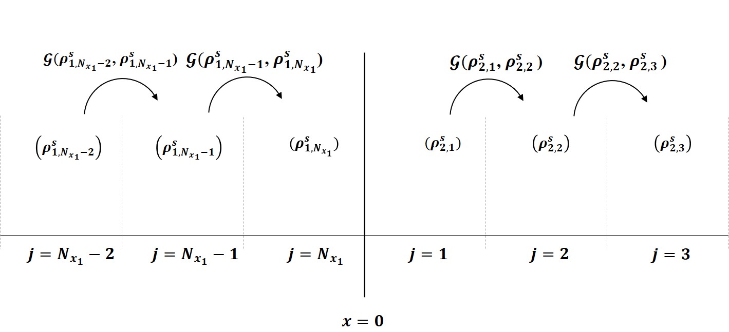
We note that the above Godunov scheme for the computation of the density values ρe,2s,,ρe,Nxe1ssuperscriptsubscript𝜌𝑒2𝑠superscriptsubscript𝜌𝑒subscript𝑁subscript𝑥𝑒1𝑠\rho_{e,2}^{s},\dots,\rho_{e,N_{x_{e}}-1}^{s} is equivalent to the cell transmission method (CTM), see [11, 15]. Figure 6(a) visualizes the fluxes at the cell interfaces. The inflow qe,ins0superscriptsubscript𝑞𝑒𝑖𝑛𝑠0q_{e,in}^{s}\geq 0 and outflow qe,outs0superscriptsubscript𝑞𝑒𝑜𝑢𝑡𝑠0q_{e,out}^{s}\geq 0 in (38) are mass fluxes at road interfaces and are determined with coupling and boundary conditions described below.

1-to-1 junction with onramp

We consider a 1-to-1 junction with an additional onramp as shown in Figure 1. We denote the incoming road with index 111 and the outgoing road with index 222. As in [19], we assume that the demand of the onramp can be controlled and apply the demand function

Dor(ls,ts)=u(ts)min{forin(ts)+lsΔt,formax},superscript𝐷orsuperscript𝑙𝑠superscript𝑡𝑠𝑢superscript𝑡𝑠superscriptsubscript𝑓orinsuperscript𝑡𝑠superscript𝑙𝑠Δ𝑡subscriptsuperscript𝑓or\displaystyle D^{\operatorname*{or}}(l^{s},t^{s})=u(t^{s})\min\Big{\{}f_{\operatorname*{or}}^{\operatorname*{in}}(t^{s})+\frac{l^{s}}{\Delta t},f^{\max}_{\operatorname*{or}}\Big{\}}, (39)

for the onramp. Here, u(t)[0,1]𝑢𝑡01u(t)\in[0,1] denotes a time-dependent metering rate which can be used to control the flow from the onramp. Moreover, formaxsubscriptsuperscript𝑓orf^{\max}_{\operatorname*{or}} is the maximum flux allowed to enter the outgoing road from the onramp. To define a unique solution, we assign priority parameters β𝛽\beta and (1β)1𝛽(1-\beta) to road e=1𝑒1e=1 and the onramp, respectively as shown in Figure 1, and compute

q1,outssuperscriptsubscript𝑞1𝑜𝑢𝑡𝑠\displaystyle q_{1,out}^{s} =min{D1LWR(ρ1,Nx1s),max{βSALWR,SALWRDor(ls,ts)}},absentsubscriptsuperscript𝐷LWR1superscriptsubscript𝜌1subscript𝑁subscript𝑥1𝑠𝛽superscript𝑆ALWRsuperscript𝑆ALWRsuperscript𝐷orsuperscript𝑙𝑠superscript𝑡𝑠\displaystyle=\min\bigg{\{}D^{\operatorname*{LWR}}_{1}(\rho_{1,N_{x_{1}}}^{s}),\max\Big{\{}\beta S^{\operatorname*{ALWR}},S^{\operatorname*{ALWR}}-D^{\operatorname*{or}}(l^{s},t^{s})\Big{\}}\bigg{\}}, (40a)
qorssuperscriptsubscript𝑞or𝑠\displaystyle q_{\operatorname*{or}}^{s} =min{Dor(ls,ts),max{(1β)SALWR,SALWRDLWR(ρ1,Nx1s)}},absentsuperscript𝐷orsuperscript𝑙𝑠superscript𝑡𝑠1𝛽superscript𝑆ALWRsuperscript𝑆ALWRsuperscript𝐷LWRsuperscriptsubscript𝜌1subscript𝑁subscript𝑥1𝑠\displaystyle=\min\bigg{\{}D^{\operatorname*{or}}(l^{s},t^{s}),\max\Big{\{}(1-\beta)S^{\operatorname*{ALWR}},S^{\operatorname*{ALWR}}-D^{\operatorname*{LWR}}(\rho_{1,N_{x_{1}}}^{s})\Big{\}}\bigg{\}}, (40b)
q2,inssuperscriptsubscript𝑞2𝑖𝑛𝑠\displaystyle q_{2,in}^{s} =q1,outs+qors,absentsuperscriptsubscript𝑞1𝑜𝑢𝑡𝑠superscriptsubscript𝑞or𝑠\displaystyle=q_{1,out}^{s}+q_{\operatorname*{or}}^{s}, (40c)

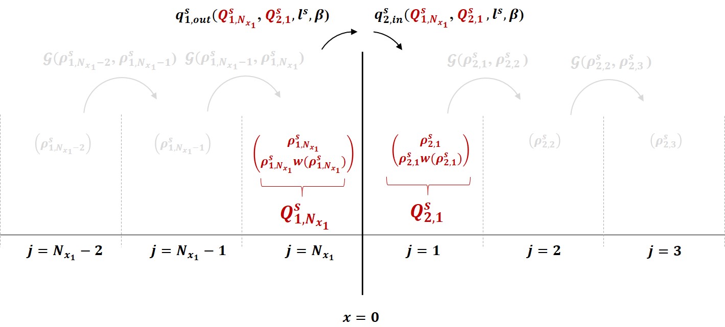
where SALWR=SALWR(ρ1,Nx1s,ρ2,1s,ls)superscript𝑆ALWRsuperscript𝑆ALWRsuperscriptsubscript𝜌1subscript𝑁subscript𝑥1𝑠superscriptsubscript𝜌21𝑠superscript𝑙𝑠S^{\operatorname*{ALWR}}=S^{\operatorname*{ALWR}}(\rho_{1,N_{x_{1}}}^{s},\rho_{2,1}^{s},l^{s}) using (16) and (28) to evaluate the ALWR supply (25). Similarly to the computation of the mass flux in a 2CTM for the second order model , which will be studied in section 4.3.1, the computation of the mass fluxes q1,outssuperscriptsubscript𝑞1𝑜𝑢𝑡𝑠q_{1,out}^{s}, qorssuperscriptsubscript𝑞or𝑠q_{\operatorname*{or}}^{s} and q2,inssuperscriptsubscript𝑞2𝑖𝑛𝑠q_{2,in}^{s} considers the w𝑤w-value of the incoming road e=1𝑒1e=1 in the supply function. This value of the mass flux is then used as input for the boundary cells, see Figure 6(b). Especially important is that the w𝑤w-value of the incoming road is derived from the density. Therefore, not the whole second order dynamics have to be tracked. We compute first order with the CTM approach and derive the second order property w𝑤w from the density.

Based on the computed fluxes, the evolution of the queue at the onramp reads

ls+1=ls+Δt(forin(ts)qors).superscript𝑙𝑠1superscript𝑙𝑠Δ𝑡superscriptsubscript𝑓orinsuperscript𝑡𝑠superscriptsubscript𝑞or𝑠\displaystyle l^{s+1}=l^{s}+\Delta t\left(f_{\operatorname*{or}}^{\operatorname*{in}}(t^{s})-q_{\operatorname*{or}}^{s}\right).

In general, we start with empty queues, i.e., l0=0superscript𝑙00l^{0}=0.

Refer to caption
(a)
Refer to caption
(b)
Figure 6: Illustration of the numerical scheme.

Onramp at origin

Additionally, we have to provide boundary data for the inflow at the beginning of the incoming road e=1𝑒1e=1. We consider an onramp at a junction with only one outgoing road, where we denote the outgoing road with the index 111. The demand function of the onramp is given by

Dor(ls,ts)={formaxif l(ts)>0,min{forin(ts)+lsΔt,formax}otherwise,superscript𝐷orsuperscript𝑙𝑠superscript𝑡𝑠casessubscriptsuperscript𝑓orif 𝑙superscript𝑡𝑠0superscriptsubscript𝑓orinsuperscript𝑡𝑠superscript𝑙𝑠Δ𝑡subscriptsuperscript𝑓orotherwise,\displaystyle D^{\operatorname*{or}}(l^{s},t^{s})=\begin{cases}f^{\max}_{\operatorname*{or}}&\text{if }l(t^{s})>0,\\ \min\{f_{\operatorname*{or}}^{\operatorname*{in}}(t^{s})+\frac{l^{s}}{\Delta t},f^{\max}_{\operatorname*{or}}\}&\text{otherwise,}\end{cases} (41)

where forin(ts)superscriptsubscript𝑓orinsuperscript𝑡𝑠f_{\operatorname*{or}}^{\operatorname*{in}}(t^{s}) is the flow of cars arriving at the onramp at time tssuperscript𝑡𝑠t^{s} and formaxsubscriptsuperscript𝑓orf^{\max}_{\operatorname*{or}} the maximum flux allowed to exit the onramp. The inflow into the system is given by

q1,ins=min{DLWR(ρ1,1s),Dor(ls,ts)}.superscriptsubscript𝑞1𝑖𝑛𝑠superscript𝐷LWRsuperscriptsubscript𝜌11𝑠superscript𝐷orsuperscript𝑙𝑠superscript𝑡𝑠\displaystyle q_{1,in}^{s}=\min\{D^{\operatorname*{LWR}}(\rho_{1,1}^{s}),D^{\operatorname*{or}}(l^{s},t^{s})\}.

Based on the computed inflow, the evolution of the queue at the onramp is given by

ls+1=ls+Δt(forin(ts)q1,ins).superscript𝑙𝑠1superscript𝑙𝑠Δ𝑡superscriptsubscript𝑓orinsuperscript𝑡𝑠superscriptsubscript𝑞1𝑖𝑛𝑠\displaystyle l^{s+1}=l^{s}+\Delta t\left(f_{\operatorname*{or}}^{\operatorname*{in}}(t^{s})-q_{1,in}^{s}\right).

Junction with outflow

At a junction with only one incoming road (denoted by index 1), we consider absorbing boundary conditions

q1,outs=min{DLWR(ρ1,Nx1s),SLWR(ρ1,Nx1s)}.superscriptsubscript𝑞1𝑜𝑢𝑡𝑠superscript𝐷LWRsuperscriptsubscript𝜌1subscript𝑁subscript𝑥1𝑠superscript𝑆LWRsuperscriptsubscript𝜌1subscript𝑁subscript𝑥1𝑠\displaystyle q_{1,out}^{s}=\min\{D^{\operatorname*{LWR}}(\rho_{1,N_{x_{1}}}^{s}),S^{\operatorname*{LWR}}(\rho_{1,N_{x_{1}}}^{s})\}.
Remark 2.

In comparison to the LWR onramp model in [19], only the supply function SALWRsuperscript𝑆ALWRS^{\operatorname*{ALWR}} on the outgoing road of the 1-to-1 junction with onramp has been adapted in the augmented model. Therefore, replacing SALWRsuperscript𝑆ALWRS^{\operatorname*{ALWR}} by SLWR(ρ2,1s)superscript𝑆LWRsuperscriptsubscript𝜌21𝑠S^{\operatorname*{LWR}}(\rho_{2,1}^{s}) in (40) gives the numerical discretization of the LWR model.

4.2 Capacity drop in comparison to the LWR model

In this section, we consider the evolution of the left- and right-hand state ρ1subscript𝜌1\rho_{1} and ρ2subscript𝜌2\rho_{2} for the Riemann problem (4) at the 1-to-1 junction with onramp, cf. Figure 1, within the ALWR model. To ensure the activation condition for the minimum in the supply function (25), we set forin(t)=formax=fmaxsuperscriptsubscript𝑓orin𝑡subscriptsuperscript𝑓orsuperscript𝑓f_{\operatorname*{or}}^{\operatorname*{in}}(t)=f^{\max}_{\operatorname*{or}}=f^{\max}. For the particular setting, solutions of Riemann problems are discussed and phase space trajectories are compared to the LWR model.

We obtain the numerical solution of the ALWR model with the scheme described in section 4.1. The only difference to the LWR network approach presented in [19] is the modelling of the supply at the junction of the network, where we impose second-order-like conditions in the supply function, cf. Section 3. The numerical solution of the LWR model is obtained as explained in remark 2. In comparison to the LWR model and as extension of the analysis in Section 3.3, the most exciting point in the ALWR model here is that the evolution of the states at the junction may lead to a change in the “active” model.
Refer to caption

(a)

Refer to caption

(b)

Refer to caption

(c)
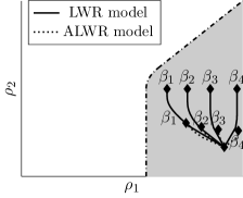
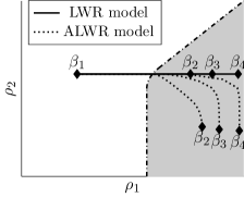
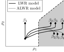
Figure 7: Comparison of the LWR and ALWR model with priority parameters β1=0.9subscript𝛽10.9\beta_{1}=0.9, β2=0.75subscript𝛽20.75\beta_{2}=0.75, β3=0.5subscript𝛽30.5\beta_{3}=0.5 and β4=0.1subscript𝛽40.1\beta_{4}=0.1.

Due to the construction of the augmented supply function within the ALWR model as minimum of the supply functions of the LWR and the ARZ model, the solution to the Riemann problem in the ALWR model is restricted by the solution in the LWR model in the sense that the (final) supply of the outgoing road is at most as large as for the same Riemann problem in the LWR model. This means that for ρ2[0,ρmax/2]subscript𝜌20superscript𝜌2\rho_{2}\in[0,\nicefrac{{\rho^{\max}}}{{2}}], the arising densities on the outgoing road can never exceed ρmax/2superscript𝜌2\nicefrac{{\rho^{\max}}}{{2}}. Analogously, for ρ2[ρmax/2,ρmax]subscript𝜌2superscript𝜌2superscript𝜌\rho_{2}\in[\nicefrac{{\rho^{\max}}}{{2}},\rho^{\max}], the density on the outgoing road can never exceed ρ2subscript𝜌2\rho_{2}. We obtain weak entropy solutions on the incoming and outgoing road, see (5). When the current densities at the left-hand and right-hand side of the junction are in a region where the LWR supply is applied, the solution is identical to the LWR model. But as soon as the combination of the density values is in the region where the ARZ supply is applied, the supply drops below the LWR supply and the models differ.

Figure 7(a) shows the phase space trajectory for a Riemann problem with ρ1[0,ρlim]subscript𝜌10subscript𝜌lim\rho_{1}\in[0,\rho_{\operatorname*{lim}}] and ρ2[ρmax/2,ρmax]subscript𝜌2superscript𝜌2superscript𝜌\rho_{2}\in[\nicefrac{{\rho^{\max}}}{{2}},\rho^{\max}] in the LWR and the ALWR model. Different priority parameters β𝛽\beta are applied at the onramp. For the choice of the priority parameter β=β1𝛽subscript𝛽1\beta=\beta_{1}, there is no restriction on the incoming road and the density at the outgoing road remains constant. Decreasing priority parameters of the first road at some point lead to congestion at the end of the first road (as it is the case for β{β2,β3,β4}𝛽subscript𝛽2subscript𝛽3subscript𝛽4\beta\in\{\beta_{2},\beta_{3},\beta_{4}\}). When the phase path enters the region where the ARZ supply is applied, the phase paths of the two models diverge. In the LWR model, only the density at the incoming road increases further. In contrast, in the ALWR model, there is a drop in the density at the outgoing road due to the congestion at the end of the incoming road. The markers at the end of each trajectory indicate the final states that are reached in the respective models for the respective priority parameters.

Figure 7(b) shows the phase space trajectory for a Riemann problem with ρ2[0,ρmax/2]subscript𝜌20superscript𝜌2\rho_{2}\in[0,\nicefrac{{\rho^{\max}}}{{2}}]. The density on the outgoing road increases up to ρmax/2superscript𝜌2\nicefrac{{\rho^{\max}}}{{2}} in the LWR model (since the accumulated demand is above fmaxsuperscript𝑓f^{\max}). In the ALWR model we see a different behavior. The density at the outgoing road increases at the beginning, but starts to drop down within the region where the ARZ supply is applied. Figure 7(c) examplarily shows some trajectories with initial data in the region where the ARZ supply is applied. The fluxes in the final situation for the examples considered before are given in Table 2. A capacity drop in the solution for the ALWR model can be seen in all of the cases where the model differs from the LWR model. Note that here, the final fluxes f2(0,T)subscript𝑓20𝑇f_{2}(0,T) at the junction match for β2,β3,β4subscript𝛽2subscript𝛽3subscript𝛽4\beta_{2},\beta_{3},\beta_{4} since the examples share the same priority parameters as well as the desired inflow from the onramp.

Table 2: Outflow f2(0,T)subscript𝑓20𝑇f_{2}(0,T) in the final state at the junction with onramp (flux values in relation to fmaxsuperscript𝑓f^{\max}).
Figure 7(a) Figure 7(b) Figure 7(c)
Priority Parameter LWR ALWR LWR ALWR LWR ALWR
β1=0.90subscript𝛽10.90\beta_{1}=0.90 0.97 0.97 1 1 1 0.84
β2=0.75subscript𝛽20.75\beta_{2}=0.75 0.97 0.81 1 0.81 1 0.81
β3=0.50subscript𝛽30.50\beta_{3}=0.50 0.97 0.78 1 0.78 1 0.78
β4=0.10subscript𝛽40.10\beta_{4}=0.10 0.97 0.77 1 0.77 1 0.77

4.3 Comparison to second order models

4.3.1 Numerical scheme for the ARZ and the Greenberg model

Within the ARZ and the Greenberg model, the traffic state Ue=(ρe,ρewe)subscript𝑈𝑒subscript𝜌𝑒subscript𝜌𝑒subscript𝑤𝑒U_{e}=(\rho_{e},\rho_{e}w_{e}), consisting of the density ρesubscript𝜌𝑒\rho_{e} and the generalized momentum ρewesubscript𝜌𝑒subscript𝑤𝑒\rho_{e}w_{e}, is computed on each road. Let Qe,jssuperscriptsubscript𝑄𝑒𝑗𝑠Q_{e,j}^{s} denote the average value of the function Ue(x,t)subscript𝑈𝑒𝑥𝑡U_{e}(x,t) on the interval Ce,jsubscript𝐶𝑒𝑗C_{e,j} at time ts=sΔtsuperscript𝑡𝑠𝑠Δ𝑡t^{s}=s\Delta t, i.e.,

Qe,js=1ΔxCe,jUe,j(x,ts)dx,superscriptsubscript𝑄𝑒𝑗𝑠1Δ𝑥subscriptsubscript𝐶𝑒𝑗subscript𝑈𝑒𝑗𝑥superscript𝑡𝑠differential-d𝑥Q_{e,j}^{s}=\frac{1}{\Delta x}\int_{C_{e,j}}U_{e,j}(x,t^{s})\mathrm{d}x,

As in [20], we apply a splitting approach consisting of a Godunov scheme for the flux term and an implicit Euler scheme for the relaxation term

Qe,1s+1=Qe,1sΔtΔx(𝒢(Qe,1s,Qe,2s)(qe,insre,ins))+Δtg(Qe,1s+1),Qe,js+1=Qe,jsΔtΔx(𝒢(Qe,js,Qe,j+1s)𝒢(Qe,j1s,Qe,js))+Δtg(Qe,js+1),j=2,,Nxe1,Qe,Nxes+1=Qe,NxesΔtΔx((qe,outsre,outs)𝒢(Qe,Nxe1s,Qe,Nxes))+Δtg(Qe,Nxes+1),\displaystyle\begin{split}Q_{e,1}^{s+1}&=Q_{e,1}^{s}-\frac{\Delta t}{\Delta x}\left(\mathcal{G}\left(Q_{e,1}^{s},Q_{e,2}^{s}\right)-\left(\begin{array}[]{c}q_{e,in}^{s}\\ r_{e,in}^{s}\end{array}\right)\right)+\Delta tg(Q_{e,1}^{s+1}),\\ Q_{e,j}^{s+1}&=Q_{e,j}^{s}-\frac{\Delta t}{\Delta x}\left(\mathcal{G}\left(Q_{e,j}^{s},Q_{e,j+1}^{s}\right)-\mathcal{G}\left(Q_{e,j-1}^{s},Q_{e,j}^{s}\right)\right)\\ &+\Delta tg(Q_{e,j}^{s+1}),\qquad j=2,\dots,N_{x_{e}}-1,\\ Q_{e,N_{x_{e}}}^{s+1}&=Q_{e,N_{x_{e}}}^{s}-\frac{\Delta t}{\Delta x}\left(\left(\begin{array}[]{c}q_{e,out}^{s}\\ r_{e,out}^{s}\end{array}\right)-\mathcal{G}\left(Q_{e,N_{x_{e}}-1}^{s},Q_{e,N_{x_{e}}}^{s}\right)\right)+\Delta tg(Q_{e,N_{x_{e}}}^{s+1}),\end{split} (42)

where there is no relaxation term for the ARZ model and for the Greenberg model, we set g(Qe,js)=(0,ρe,js(ve,jsV(ρe,js))/τ)T𝑔superscriptsubscript𝑄𝑒𝑗𝑠superscript0superscriptsubscript𝜌𝑒𝑗𝑠superscriptsubscript𝑣𝑒𝑗𝑠𝑉superscriptsubscript𝜌𝑒𝑗𝑠𝜏𝑇g(Q_{e,j}^{s})=(0,\nicefrac{{-\rho_{e,j}^{s}(v_{e,j}^{s}-V(\rho_{e,j}^{s}))}}{{\tau}})^{T} equal to the right-hand side of the relaxed system (24). The vectors (qe,ins,re,ins)Tsuperscriptsuperscriptsubscript𝑞𝑒𝑖𝑛𝑠superscriptsubscript𝑟𝑒𝑖𝑛𝑠𝑇(q_{e,in}^{s},r_{e,in}^{s})^{T} and (qe,outs,re,outs)Tsuperscriptsuperscriptsubscript𝑞𝑒𝑜𝑢𝑡𝑠superscriptsubscript𝑟𝑒𝑜𝑢𝑡𝑠𝑇(q_{e,out}^{s},r_{e,out}^{s})^{T} in (42) denote mass and momentum flux at the road interfaces. The Godunov flux for the second order system formulated with the ARZ demand and supply functions (14)-(15) is given by

𝒢(Qe,js,Qe,j+1s)𝒢superscriptsubscript𝑄𝑒𝑗𝑠superscriptsubscript𝑄𝑒𝑗1𝑠\displaystyle\mathcal{G}\left(Q_{e,j}^{s},Q_{e,j+1}^{s}\right) =(1we,js)min{DARZ(ρe,js,we,js),SARZ(ρ~e,j+1s,we,js)},absent1superscriptsubscript𝑤𝑒𝑗𝑠superscript𝐷ARZsuperscriptsubscript𝜌𝑒𝑗𝑠superscriptsubscript𝑤𝑒𝑗𝑠superscript𝑆ARZsuperscriptsubscript~𝜌𝑒𝑗1𝑠superscriptsubscript𝑤𝑒𝑗𝑠\displaystyle=\left(\begin{array}[]{c}1\\ w_{e,j}^{s}\end{array}\right)\min\{D^{\operatorname*{ARZ}}\left(\rho_{e,j}^{s},w_{e,j}^{s}\right),S^{\operatorname*{ARZ}}\left(\tilde{\rho}_{e,j+1}^{s},w_{e,j}^{s}\right)\},

where the intermediate state Q~e,j+1s=(ρ~e,j+1s,ρ~e,j+1swe,js)Tsuperscriptsubscript~𝑄𝑒𝑗1𝑠superscriptsuperscriptsubscript~𝜌𝑒𝑗1𝑠superscriptsubscript~𝜌𝑒𝑗1𝑠superscriptsubscript𝑤𝑒𝑗𝑠𝑇\tilde{Q}_{e,j+1}^{s}=(\tilde{\rho}_{e,j+1}^{s},\tilde{\rho}_{e,j+1}^{s}w_{e,j}^{s})^{T} used to evaluate the supply is such that

ρ~e,j+1s=p1(max{we,jsve,j+1s,0}).superscriptsubscript~𝜌𝑒𝑗1𝑠superscript𝑝1superscriptsubscript𝑤𝑒𝑗𝑠superscriptsubscript𝑣𝑒𝑗1𝑠0\tilde{\rho}_{e,j+1}^{s}=p^{-1}\left(\max\{w_{e,j}^{s}-v_{e,j+1}^{s},0\}\right).

In the following, we explain how the flux terms for the inflow and the outflow are given by coupling and boundary conditions.

Onramp at origin

We model a junction with an onramp at the beginning of the network similar as in the first order model. For the onramp with queue length lssuperscript𝑙𝑠l^{s} at time tssuperscript𝑡𝑠t^{s}, we use the demand function (41) to determine the mass flow q1,inssuperscriptsubscript𝑞1𝑖𝑛𝑠q_{1,in}^{s}. However, due to the second order system, we have to provide also boundary data for the momentum flow. We follow the idea introduced by [20] to compute the w𝑤w-value at the boundary. We compute

ρs=ρmax2(ρmax2)2ρmaxDor(ls,ts)vmax.superscriptsubscript𝜌𝑠superscript𝜌2superscriptsuperscript𝜌22superscript𝜌superscript𝐷orsuperscript𝑙𝑠superscript𝑡𝑠superscript𝑣\rho_{-}^{s}=\frac{\rho^{\max}}{2}-\sqrt{\left(\frac{\rho^{\max}}{2}\right)^{2}-\frac{\rho^{\max}D^{\operatorname*{or}}(l^{s},t^{s})}{v^{\max}}}.

Let ws=w(ρs)=V(ρs)+p(ρs)superscriptsubscript𝑤𝑠𝑤superscriptsubscript𝜌𝑠𝑉superscriptsubscript𝜌𝑠𝑝superscriptsubscript𝜌𝑠w_{-}^{s}=w(\rho_{-}^{s})=V(\rho_{-}^{s})+p(\rho_{-}^{s}), then we can model the boundary fluxes by

(q1,insr1,ins)=(1ws)min{Dor(ls,ts),SARZ(ρ~1,0s,ws)},superscriptsubscript𝑞1𝑖𝑛𝑠superscriptsubscript𝑟1𝑖𝑛𝑠1superscriptsubscript𝑤𝑠superscript𝐷orsuperscript𝑙𝑠superscript𝑡𝑠superscript𝑆ARZsuperscriptsubscript~𝜌10𝑠superscriptsubscript𝑤𝑠\left(\begin{array}[]{c}q_{1,in}^{s}\\ r_{1,in}^{s}\end{array}\right)=\left(\begin{array}[]{c}1\\ w_{-}^{s}\end{array}\right)\min\Big{\{}D^{\operatorname*{or}}(l^{s},t^{s}),S^{\operatorname*{ARZ}}(\tilde{\rho}_{1,0}^{s},w_{-}^{s})\Big{\}},

with ρ~1,0s=p1(max{wsv1,1s,0})superscriptsubscript~𝜌10𝑠superscript𝑝1superscriptsubscript𝑤𝑠superscriptsubscript𝑣11𝑠0\tilde{\rho}_{1,0}^{s}=p^{-1}\left(\max\{w_{-}^{s}-v_{1,1}^{s},0\}\right).

1-to-1 junction with onramp

At the 1-to-1 junction with onramp, we denote the incoming road e=1𝑒1e=1 and outgoing road e=2𝑒2e=2. We assume that the onramp can be controlled by the time–dependent metering rate u(t)𝑢𝑡u(t) and compute the controlled onramp demand with equation (39). The fluxes at the road interfaces are given by

(q1,outsr1,outs)superscriptsubscript𝑞1𝑜𝑢𝑡𝑠superscriptsubscript𝑟1𝑜𝑢𝑡𝑠\displaystyle\left(\begin{array}[]{c}q_{1,out}^{s}\\ r_{1,out}^{s}\end{array}\right) =(1w1,Nx1s)min{D1,max{βS2,S2Dor(ls,ts)}},absent1superscriptsubscript𝑤1subscript𝑁subscript𝑥1𝑠subscript𝐷1𝛽subscript𝑆2subscript𝑆2superscript𝐷orsuperscript𝑙𝑠superscript𝑡𝑠\displaystyle=\left(\begin{array}[]{c}1\\ w_{1,N_{x_{1}}}^{s}\end{array}\right)\min\bigg{\{}D_{1},\max\Big{\{}\beta S_{2},S_{2}-D^{\operatorname*{or}}(l^{s},t^{s})\Big{\}}\bigg{\}},
(qor,outsror,outs)superscriptsubscript𝑞or𝑜𝑢𝑡𝑠superscriptsubscript𝑟or𝑜𝑢𝑡𝑠\displaystyle\left(\begin{array}[]{c}q_{\operatorname*{or},out}^{s}\\ r_{\operatorname*{or},out}^{s}\end{array}\right) =(1w1,Nx1s)min{Dor(ls,ts),max{(1β)S2,S2D1}},absent1superscriptsubscript𝑤1subscript𝑁subscript𝑥1𝑠superscript𝐷orsuperscript𝑙𝑠superscript𝑡𝑠1𝛽subscript𝑆2subscript𝑆2subscript𝐷1\displaystyle=\left(\begin{array}[]{c}1\\ w_{1,N_{x_{1}}}^{s}\end{array}\right)\min\bigg{\{}D^{\operatorname*{or}}(l^{s},t^{s}),\max\Big{\{}\Big{(}1-\beta)S_{2},S_{2}-D_{1}\}\bigg{\}},
(q2,inr2,in)subscript𝑞2𝑖𝑛subscript𝑟2𝑖𝑛\displaystyle\left(\begin{array}[]{c}q_{2,in}\\ r_{2,in}\end{array}\right) =(1w1,Nx1s)(q1,outs+qor,outs),absent1superscriptsubscript𝑤1subscript𝑁subscript𝑥1𝑠superscriptsubscript𝑞1𝑜𝑢𝑡𝑠superscriptsubscript𝑞or𝑜𝑢𝑡𝑠\displaystyle=\left(\begin{array}[]{c}1\\ w_{1,N_{x_{1}}}^{s}\end{array}\right)(q_{1,out}^{s}+q_{\operatorname*{or},out}^{s}),

where

D1=DARZ(ρ1,Nx1s,w1,Nx1s),S2=SARZ(ρ~2,1s,w1,Nx1s),ρ~2,1s=p1(max{w1,Nx1sv2,1s,0})formulae-sequencesubscript𝐷1superscript𝐷ARZsuperscriptsubscript𝜌1subscript𝑁subscript𝑥1𝑠superscriptsubscript𝑤1subscript𝑁subscript𝑥1𝑠formulae-sequencesubscript𝑆2superscript𝑆ARZsuperscriptsubscript~𝜌21𝑠superscriptsubscript𝑤1subscript𝑁subscript𝑥1𝑠superscriptsubscript~𝜌21𝑠superscript𝑝1superscriptsubscript𝑤1subscript𝑁subscript𝑥1𝑠superscriptsubscript𝑣21𝑠0D_{1}=D^{\operatorname*{ARZ}}(\rho_{1,N_{x_{1}}}^{s},w_{1,N_{x_{1}}}^{s}),\qquad S_{2}=S^{\operatorname*{ARZ}}(\tilde{\rho}_{2,1}^{s},w_{1,N_{x_{1}}}^{s}),\qquad\tilde{\rho}_{2,1}^{s}=p^{-1}\left(\max\{w_{1,N_{x_{1}}}^{s}-v_{2,1}^{s},0\}\right)

Junction with outflow

At a junction with only one incoming road (denoted by index 1), we consider absorbing boundary conditions. We have

(q1,outsr1,outs)superscriptsubscript𝑞1𝑜𝑢𝑡𝑠superscriptsubscript𝑟1𝑜𝑢𝑡𝑠\displaystyle\left(\begin{array}[]{c}q_{1,out}^{s}\\ r_{1,out}^{s}\end{array}\right) =(1wNx11s)min{DARZ(ρNx11s,wNx11s),SARZ(ρNx11s,wNx11s)}.absent1superscriptsubscript𝑤subscript𝑁subscript𝑥11𝑠superscript𝐷ARZsuperscriptsubscript𝜌subscript𝑁subscript𝑥11𝑠superscriptsubscript𝑤subscript𝑁subscript𝑥11𝑠superscript𝑆ARZsuperscriptsubscript𝜌subscript𝑁subscript𝑥11𝑠superscriptsubscript𝑤subscript𝑁subscript𝑥11𝑠\displaystyle=\left(\begin{array}[]{c}1\\ w_{N_{x_{1}}-1}^{s}\end{array}\right)\min\Big{\{}D^{\operatorname*{ARZ}}\left(\rho_{N_{x_{1}}-1}^{s},w_{N_{x_{1}}-1}^{s}\right),S^{\operatorname*{ARZ}}\left(\rho_{N_{x_{1}}-1}^{s},w_{N_{x_{1}}-1}^{s}\right)\Big{\}}.

Analogously to Godunov scheme for the first order models, the Godunov approximation for the second order models is mathematically equivalent to a cell transmission model (2CTM), see [15], using the supply function of the ARZ model and the two quantities ρ𝜌\rho, w𝑤w.

4.3.2 Capacity drop in comparison to second order models

We consider the network depicted in Figure 1 with the parameters given in Table 3, which are inspired by the onramp scenario in [20, Section 4.3]. We set Δx=0.25kmΔ𝑥0.25km\Delta x=0.25\,\text{km}, Δt=2103hΔ𝑡2superscript103h\Delta t=2\cdot 10^{-3}\,\text{h} and the desired inflow from the onramp to forin=4000carshsuperscriptsubscript𝑓orin4000carshf_{\operatorname*{or}}^{\operatorname*{in}}=4000\,\frac{\text{cars}}{\text{h}} and the maximum flux allowed to exit the onramp equal to the maximum flux of the outgoing road formax=4500carshsubscriptsuperscript𝑓or4500carshf^{\max}_{\operatorname*{or}}=4500\,\frac{\text{cars}}{\text{h}}. The priority is β=0.5𝛽0.5\beta=0.5 and the incoming road therefore experiences congestion. We compute the time evolution of the (half-) Riemann problem (4) with ρ10=140superscriptsubscript𝜌10140\rho_{1}^{0}=140, ρ20=90superscriptsubscript𝜌2090\rho_{2}^{0}=90 within the LWR and ALWR model. Within the ARZ and the Greenberg model, we compute the time evolution of the (half-) Riemann problem (13) with initial states (ρ10,w10)superscriptsubscript𝜌10superscriptsubscript𝑤10(\rho_{1}^{0},w_{1}^{0}), (ρ20,w20)superscriptsubscript𝜌20superscriptsubscript𝑤20(\rho_{2}^{0},w_{2}^{0}) where we0=V(ρe0)+p(ρe0)superscriptsubscript𝑤𝑒0𝑉superscriptsubscript𝜌𝑒0𝑝superscriptsubscript𝜌𝑒0w_{e}^{0}=V(\rho_{e}^{0})+p(\rho_{e}^{0}), e=1,2𝑒12e=1,2.

The density at the end of the incoming road increases in all models, see Figure 8(a). The density in the Greenberg model increases similar to the ARZ model but is relaxed towards the ALWR flux as time progresses. The discharge flow of the junction in the LWR model stays at the level of the maximum flow even as further congestion on the incoming road sets on, compare Figure 8(b). In contrast, all of the other models predict a decrease in the discharge flow at the junction. At t=0𝑡0t=0, the flux (ρv)2(0,0)subscript𝜌𝑣200(\rho v)_{2}(0,0) is identical for the Greenberg and the ARZ model. However, the flux in the Greenberg model is relaxed until a state on the LWR fundamental diagram is reached. The ALWR model mimics the flux of the second order model at the junction. We see a capacity drop since the discharge flow is lower than the maximum flux due to congestion on the incoming road.

Table 3: Properties of the roads in Figure 1.
road length [km]delimited-[]km[\text{km}] ρmaxsuperscript𝜌\rho^{\max} [carskm]delimited-[]carskm[\frac{\text{cars}}{\text{km}}] vmaxsuperscript𝑣v^{\max} [kmh]delimited-[]kmh[\frac{\text{km}}{\text{h}}] initial density ρ0superscript𝜌0\rho^{0} [carskm]delimited-[]carskm[\frac{\text{cars}}{\text{km}}]
road 111 4 180 100 140
road 222 2 180 100 90

Refer to caption

Refer to caption

(a)

Refer to caption

(b)
Figure 8: Densities and fluxes.

4.3.3 The ramp metering control problem

We consider an onramp with ramp metering as introduced in Section 4.1 and 4.3.1 with a piecewise constant control function u(t)𝑢𝑡u(t) on intervals of 15 minutes. Our aim is to compare the optimal control of the ALWR model with optimal control results of the Greenberg model. We consider the relaxation time τ=0.005h𝜏0.005h\tau=0.005\,\text{h} for the Greenberg model (24) and the parameters from Table 3 but set the initial densities to ρe0=50carskmsuperscriptsubscript𝜌𝑒050carskm\rho_{e}^{0}=50\frac{\text{cars}}{\text{km}}, e=1,2𝑒12e=1,2 such that both roads have equal traffic volume at t=0𝑡0t=0. The priority parameter β𝛽\beta at the onramp equals 0.5 and we set the maximum inflow from the onramp to formax=2000carshsubscriptsuperscript𝑓or2000carshf^{\max}_{\operatorname*{or}}=2000\,\frac{\text{cars}}{\text{h}}. Additionally, we consider an onramp at the origin in with formax=4500carshsubscriptsuperscript𝑓or4500carshf^{\max}_{\operatorname*{or}}=4500\,\frac{\text{cars}}{\text{h}}. The time horizon is T=3𝑇3T=3 hours. The applied discretization parameters are Δx=0.25kmΔ𝑥0.25km\Delta x=0.25\,\text{km} and Δt=2103hΔ𝑡2superscript103h\Delta t=2\cdot 10^{-3}\,\text{h} and we apply the discretization schemes described in section 4.1 and 4.3.1.

For the control scenario, we apply the inflow conditions shown in Figure 9(a). At the beginning of the time horizon, we consider a first rush-hour with moderate demand at the onramp. Later on, we consider a second rush-hour, with increased onramp demand. For the given scenario, we are interested in minimizing the total travel time

e=120T0Leρe(x,t)dxdt+e=120Tle(t)dt,superscriptsubscript𝑒12superscriptsubscript0𝑇superscriptsubscript0subscript𝐿𝑒subscript𝜌𝑒𝑥𝑡differential-d𝑥differential-d𝑡superscriptsubscript𝑒12superscriptsubscript0𝑇subscript𝑙𝑒𝑡differential-d𝑡\sum\limits_{e=1}^{2}\int\limits_{0}^{T}\int\limits_{0}^{L_{e}}\rho_{e}(x,t)\,\mathrm{d}x\,\mathrm{d}t\ +\sum\limits_{e=1}^{2}\int\limits_{0}^{T}l_{e}(t)\,\mathrm{d}t, (43)

where l1subscript𝑙1l_{1} denotes the queue at in and l2subscript𝑙2l_{2} the queue at ramp. To solve this optimization task, we apply a first-discretize-then-optimize approach. Thus, for given control decisions (time-dependent piecewise constant metering rates), the discretization schemes are always used to evaluate the objective function (43). The Matlab solver fmincon222https://de.mathworks.com/help/optim/ug/fmincon.html is used for the optimization of the control decisions.
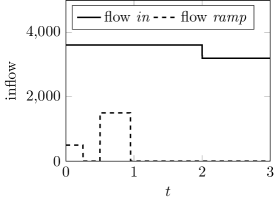
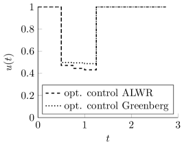
Refer to caption

(a)

Refer to caption

(b)
Figure 9: Inflow and controls.
Table 4: Optimization results (total travel time) for the network in Figure 1.
Greenberg ALWR LWR
no control 1236.5 1316.0 1019.3
optimal control ALWR 996.6 1019.6 1019.6
optimal control Greenberg 1982.3 1322.9 1019.5

Table 4 shows the total travel times for the different models with and without optimization (u(t)=1t𝑢𝑡1for-all𝑡u(t)=1~{}\forall t). The resulting queues are shown in Figure 10, where we show the Greenberg model to demonstrate the benefit of the optimized control computed with the cheaper ALWR model.

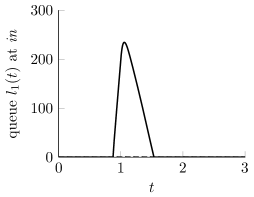
Refer to caption

Refer to caption

(a)

Refer to caption

(b)
Figure 10: Queues in the Greenberg model with and without optimization.

Running a simulation with the Greenberg model using the optimal control of the ALWR model leads to a total travel time of 996.6, which is about 1.5% away from the optimal solution found by optimizing the Greenberg model, see Table 4. Actually, the optimal metering rates for the two models do not differ much, see Figure 9(b). The key in improving the travel times is the reduction of the flow from the onramp in the time frame of high onramp demand, compare Figure 9. Both controls do not reduce the onramp demand during the first rush-hour, but reduce it during the second rush-hour to ensure that the incoming road stays in free flow. Without control, the queue at the onramp stays empty whereas more than 200 cars accumulate in the queue at the origin, see Figure 10. When the optimal control of the Greenberg or the ALWR model is used, the queue at the origin is reduced to zero, while the cars accumulate in the queue at the onramp during the rush-hour time. Ramp metering leads to an increased outflow at the end of the outgoing road early within the time horizon, see Figure 11. Note that an optimal control strategy cannot be recognized by an optimal control approach based on the LWR model since full inflow, i.e., u(t)=1t𝑢𝑡1for-all𝑡u(t)=1~{}\forall t is optimal for the LWR model. However, this is clearly not optimal for the Greenberg model, see Table 4.

Refer to caption

Refer to caption

(a)

Refer to caption

(b)
Figure 11: Flow at the end of the outgoing road out with and without optimization.

5 Conclusion

We have established a new model for the 1-to-1 junction with onramp which couples the LWR model to boundary conditions of the second order traffic model. The main difference to earlier presented versions of the LWR model is the shape of the supply function at the junction, which allows for formation of congestion when the incoming road is congested. A discussion of the new supply function was presented and we have shown that the fluxes at the junctions are only dependent on the densities of the adjacent roads. Numerical studies have shown that the ALWR model is able to capture the capacity drop phenomenon. Even though the junction model is a modification of the most simple traffic model for traffic flows, we achieved promising results and were able to capture at least some aspects of second order traffic models. Optimization results showed that the ALWR model is a suitable surrogate for the Greenberg model. In the considered scenario, the ALWR model optimum is close to the optimum of the Greenberg model. Note that similar considerations can be done analogously for exponents γ>1𝛾1\gamma>1 in the pressure function which is postponed to future work.

Acknowledgment

This work was supported by the DFG grant No. GO 1920/7-1 and by DAAD (Project-ID 57445223).

6 Appendix

We begin with some general observations which are useful to derive the partitioning of the ρ1subscript𝜌1\rho_{1}-ρ2subscript𝜌2\rho_{2}-plane in Figure 5. For fixed ρ1subscript𝜌1\rho_{1}, the value of ρ~~𝜌\tilde{\rho} given by (28) increases with ρ2subscript𝜌2\rho_{2}

ρ2ρ~0.subscriptsubscript𝜌2~𝜌0\partial_{\rho_{2}}\tilde{\rho}\geq 0. (44)

Moreover, due to (44), the partial derivative for the density on the outgoing road of the derived ARZ supply (27) satisfies

ρ2SARZ(ρ1,ρ2)0.subscriptsubscript𝜌2superscript𝑆ARZsubscript𝜌1subscript𝜌20\partial_{\rho_{2}}S^{\operatorname*{ARZ}}(\rho_{1},\rho_{2})\leq 0. (45)

Thus, the larger ρ2subscript𝜌2\rho_{2}, the larger ρ~~𝜌\tilde{\rho} and the lower the ARZ supply. Furthermore, for ρ1=ρ2subscript𝜌1subscript𝜌2\rho_{1}=\rho_{2}, we have ρ~=ρ1=ρ2~𝜌subscript𝜌1subscript𝜌2\tilde{\rho}=\rho_{1}=\rho_{2}. Now, we have a closer look at ρ~~𝜌\tilde{\rho} for ρ2ρ1subscript𝜌2subscript𝜌1\rho_{2}\geq\rho_{1}. We show that

ρ~=p1(p(ρ1)+V1V2)ρ2.~𝜌superscript𝑝1𝑝subscript𝜌1subscript𝑉1subscript𝑉2subscript𝜌2\tilde{\rho}=p^{-1}\left(p(\rho_{1})+V_{1}-V_{2}\right)\geq\rho_{2}. (46)

This is equivalent to

p(ρ1)+V1V2𝑝subscript𝜌1subscript𝑉1subscript𝑉2\displaystyle p(\rho_{1})+V_{1}-V_{2} p(ρ2)absent𝑝subscript𝜌2\displaystyle\geq p(\rho_{2})
vmax(ρ2ρ1ρmax+ρ122(ρmax)2)superscript𝑣subscript𝜌2subscript𝜌1superscript𝜌superscriptsubscript𝜌122superscriptsuperscript𝜌2\displaystyle v^{\max}\left(\frac{\rho_{2}-\rho_{1}}{\rho^{\max}}+\frac{\rho_{1}^{2}}{2\left(\rho^{\max}\right)^{2}}\right) vmax2(ρ2ρmax)2absentsuperscript𝑣2superscriptsubscript𝜌2superscript𝜌2\displaystyle\geq\frac{v^{\max}}{2}\left(\frac{\rho_{2}}{{\rho^{\max}}}\right)^{2}
ρ2ρ1ρmaxsubscript𝜌2subscript𝜌1superscript𝜌\displaystyle\frac{\rho_{2}-\rho_{1}}{\rho^{\max}} ρ22ρ122(ρmax)2absentsuperscriptsubscript𝜌22superscriptsubscript𝜌122superscriptsuperscript𝜌2\displaystyle\geq\frac{\rho_{2}^{2}-\rho_{1}^{2}}{2{\left(\rho^{\max}\right)}^{2}}
2ρmax2superscript𝜌\displaystyle 2\rho^{\max} ρ1+ρ2,absentsubscript𝜌1subscript𝜌2\displaystyle\geq\rho_{1}+\rho_{2},

which is satisfied for any combination (ρ1,ρ2)[0,ρmax]2subscript𝜌1subscript𝜌2superscript0superscript𝜌2(\rho_{1},\rho_{2})\in[0,\rho^{\max}]^{2}. In the following, we prove the partitioning of the ρ1subscript𝜌1\rho_{1}-ρ2subscript𝜌2\rho_{2}-plane.

I

The analysis for

ρ1>ρlim,ρ2ρmax2,formulae-sequencesubscript𝜌1subscript𝜌limsubscript𝜌2superscript𝜌2\rho_{1}>\rho_{\operatorname*{lim}},\qquad\rho_{2}\leq\frac{\rho^{\max}}{2},

is straightforward. The area of admissible combinations (ρ1,ρ2)subscript𝜌1subscript𝜌2(\rho_{1},\rho_{2}) is shown in area I of Figure 5. By the definition of ρlimsubscript𝜌lim\rho_{\operatorname*{lim}}, cf. equation (29), it holds that

SLWR(ρ2)=fmax>SARZ(ρ1,0).superscript𝑆LWRsubscript𝜌2superscript𝑓superscript𝑆ARZsubscript𝜌10\displaystyle S^{\operatorname*{LWR}}(\rho_{2})=f^{\max}>S^{\operatorname*{ARZ}}(\rho_{1},0).

Therefore, SLWR(ρ2)>SARZ(ρ1,ρ2)superscript𝑆LWRsubscript𝜌2superscript𝑆ARZsubscript𝜌1subscript𝜌2S^{\operatorname*{LWR}}(\rho_{2})>S^{\operatorname*{ARZ}}(\rho_{1},\rho_{2}) holds and the ARZ supply is applied.

VII

We analyze more closely the case

ρ1ρlim,subscript𝜌1subscript𝜌lim\rho_{1}\leq\rho_{\operatorname*{lim}},

which is the area VII in Figure 5. By the definition of ρlimsubscript𝜌lim\rho_{\operatorname*{lim}}, cf. equation (29), we have that SARZ(ρ1,0)fmaxsuperscript𝑆ARZsubscript𝜌10superscript𝑓S^{\operatorname*{ARZ}}(\rho_{1},0)\geq f^{\max}.

  • a)

    Assume first that ρ1ρ2subscript𝜌1subscript𝜌2\rho_{1}\geq\rho_{2}. Then

    ρ~=p1(max{0,V1V2+p(ρ1)})ρ1<(ρ1),~𝜌superscript𝑝10subscript𝑉1subscript𝑉2𝑝subscript𝜌1subscript𝜌1subscript𝜌1\tilde{\rho}=p^{-1}\left(\max\{0,V_{1}-V_{2}+p(\rho_{1})\}\right)\leq\rho_{1}<\mathcal{M}(\rho_{1}),

    and this leads to

    SARZ(ρ1,ρ2)=SARZ(ρ1,0)fmaxSLWR(ρ2).superscript𝑆ARZsubscript𝜌1subscript𝜌2superscript𝑆ARZsubscript𝜌10superscript𝑓superscript𝑆LWRsubscript𝜌2S^{\operatorname*{ARZ}}(\rho_{1},\rho_{2})=S^{\operatorname*{ARZ}}(\rho_{1},0)\geq f^{\max}\geq S^{\operatorname*{LWR}}(\rho_{2}).
  • b)

    Assume now ρ2>ρ1subscript𝜌2subscript𝜌1\rho_{2}>\rho_{1} and ρ2ρmax/2subscript𝜌2superscript𝜌2\rho_{2}\geq\nicefrac{{\rho^{\max}}}{{2}}.

    • b1)

      Assume ρ~σ1~𝜌subscript𝜎1\tilde{\rho}\geq\sigma_{1}. Then we have

      SARZ(ρ1,ρ2)=ρ~(w1(w1V2))=ρ~V2ρ2V2=SLWR(ρ2),superscript𝑆ARZsubscript𝜌1subscript𝜌2~𝜌subscript𝑤1subscript𝑤1subscript𝑉2~𝜌subscript𝑉2subscript𝜌2subscript𝑉2superscript𝑆LWRsubscript𝜌2S^{\operatorname*{ARZ}}(\rho_{1},\rho_{2})=\tilde{\rho}(w_{1}-(w_{1}-V_{2}))=\tilde{\rho}V_{2}\geq\rho_{2}V_{2}=S^{\operatorname*{LWR}}(\rho_{2}),

      where we made use of the relation of ρ~~𝜌\tilde{\rho} and ρ2subscript𝜌2\rho_{2} in equation (46).

    • b2)

      If instead we have ρ~<σ1~𝜌subscript𝜎1\tilde{\rho}<\sigma_{1}, then

      SARZ(ρ1,ρ2)=SARZ(ρ1,0)SLWR(ρ2),superscript𝑆ARZsubscript𝜌1subscript𝜌2superscript𝑆ARZsubscript𝜌10superscript𝑆LWRsubscript𝜌2S^{\operatorname*{ARZ}}(\rho_{1},\rho_{2})=S^{\operatorname*{ARZ}}(\rho_{1},0)\geq S^{\operatorname*{LWR}}(\rho_{2}),

      due to the assumption ρ1ρlimsubscript𝜌1subscript𝜌lim\rho_{1}\leq\rho_{\operatorname*{lim}}.

  • c)

    Assume ρ2>ρ1subscript𝜌2subscript𝜌1\rho_{2}>\rho_{1} and ρ2<ρmax/2subscript𝜌2superscript𝜌2\rho_{2}<\nicefrac{{\rho^{\max}}}{{2}}. From a) and b), we deduce

    SARZ(ρ1,ρmax2)fmax,ρ1[0,ρlim].formulae-sequencesuperscript𝑆ARZsubscript𝜌1superscript𝜌2superscript𝑓for-allsubscript𝜌10subscript𝜌limS^{\operatorname*{ARZ}}\left(\rho_{1},\frac{\rho^{\max}}{2}\right)\geq f^{\max},\qquad\forall\rho_{1}\in[0,\rho_{\operatorname*{lim}}].

    Moreover since (45) holds true, we know that

    SARZ(ρ1,ρ2)fmax=SLWR(ρ2),ρ1[0,ρlim],ρ2(ρ1,ρmax2).formulae-sequencesuperscript𝑆ARZsubscript𝜌1subscript𝜌2superscript𝑓superscript𝑆LWRsubscript𝜌2formulae-sequencefor-allsubscript𝜌10subscript𝜌limsubscript𝜌2subscript𝜌1superscript𝜌2S^{\operatorname*{ARZ}}(\rho_{1},\rho_{2})\geq f^{\max}=S^{\operatorname*{LWR}}(\rho_{2}),\qquad\forall\rho_{1}\in[0,\rho_{\operatorname*{lim}}],~{}\rho_{2}\in\left(\rho_{1},\frac{\rho^{\max}}{2}\right).
II

Let (ρ1,ρ2)subscript𝜌1subscript𝜌2(\rho_{1},\rho_{2}) be given with

ρ1>ρlim,ρ2>ρmax2,ρ2<σ1,SARZ(ρ1,0)SLWR(ρ2).formulae-sequencesubscript𝜌1subscript𝜌limformulae-sequencesubscript𝜌2superscript𝜌2formulae-sequencesubscript𝜌2subscript𝜎1superscript𝑆ARZsubscript𝜌10superscript𝑆LWRsubscript𝜌2\rho_{1}>\rho_{\operatorname*{lim}},\qquad\rho_{2}>\frac{\rho^{\max}}{2},\qquad\rho_{2}<\sigma_{1},\qquad S^{\operatorname*{ARZ}}(\rho_{1},0)\geq S^{\operatorname*{LWR}}(\rho_{2}).

Because ρ2<σ1subscript𝜌2subscript𝜎1\rho_{2}<\sigma_{1}, we get the inequality ρ2<(ρ1)subscript𝜌2subscript𝜌1\rho_{2}<\mathcal{M}(\rho_{1}) from (35). Moreover due to SARZ(ρ1,0)SLWR(ρ2)superscript𝑆ARZsubscript𝜌10superscript𝑆LWRsubscript𝜌2S^{\operatorname*{ARZ}}(\rho_{1},0)\geq S^{\operatorname*{LWR}}(\rho_{2}), compare (36), we know from (37) that ρ2𝒲(ρ1)subscript𝜌2𝒲subscript𝜌1\rho_{2}\geq\mathcal{W}(\rho_{1}). This gives the area II in the ρ1subscript𝜌1\rho_{1}-ρ2subscript𝜌2\rho_{2}-plane in Figure 5. For given (ρ1,ρ2)subscript𝜌1subscript𝜌2(\rho_{1},\rho_{2}) in area II, we have to proof that the LWR model is applied. We can proceed similarly as for region VII:

For ρ1ρ2subscript𝜌1subscript𝜌2\rho_{1}\geq\rho_{2}, it holds that ρ~ρ1(ρ1)~𝜌subscript𝜌1subscript𝜌1\tilde{\rho}\leq\rho_{1}\leq\mathcal{M}(\rho_{1}) and SARZ(ρ1,ρ2)=SARZ(ρ1,0)SLWR(ρ2)superscript𝑆ARZsubscript𝜌1subscript𝜌2superscript𝑆ARZsubscript𝜌10superscript𝑆LWRsubscript𝜌2S^{\operatorname*{ARZ}}(\rho_{1},\rho_{2})=S^{\operatorname*{ARZ}}(\rho_{1},0)\geq S^{\operatorname*{LWR}}(\rho_{2}).

For ρ2>ρ1ρmax/2subscript𝜌2subscript𝜌1superscript𝜌2\rho_{2}>\rho_{1}\geq\nicefrac{{\rho^{\max}}}{{2}}, we distinguish again. If ρ~σ1~𝜌subscript𝜎1\tilde{\rho}\geq\sigma_{1}, then SARZ(ρ1,ρ2)=ρ~V2ρ2V2superscript𝑆ARZsubscript𝜌1subscript𝜌2~𝜌subscript𝑉2subscript𝜌2subscript𝑉2S^{\operatorname*{ARZ}}(\rho_{1},\rho_{2})=\tilde{\rho}V_{2}\geq\rho_{2}V_{2}. If instead ρ~<σ1~𝜌subscript𝜎1\tilde{\rho}<\sigma_{1}, then SARZ(ρ1,ρ2)=SARZ(ρ1,0)SLWR(ρ2)superscript𝑆ARZsubscript𝜌1subscript𝜌2superscript𝑆ARZsubscript𝜌10superscript𝑆LWRsubscript𝜌2S^{\operatorname*{ARZ}}(\rho_{1},\rho_{2})=S^{\operatorname*{ARZ}}(\rho_{1},0)\geq S^{\operatorname*{LWR}}(\rho_{2}).

IV

Let (ρ1,ρ2)subscript𝜌1subscript𝜌2(\rho_{1},\rho_{2}) satisfy the assumptions

ρ1>ρlim,ρ2>ρmax2,ρ2σ1,ρ1ρ2.formulae-sequencesubscript𝜌1subscript𝜌limformulae-sequencesubscript𝜌2superscript𝜌2formulae-sequencesubscript𝜌2subscript𝜎1subscript𝜌1subscript𝜌2\rho_{1}>\rho_{\operatorname*{lim}},\qquad\rho_{2}>\frac{\rho^{\max}}{2},\qquad\rho_{2}\geq\sigma_{1},\qquad\rho_{1}\leq\rho_{2}.

The area for admissible values of ρ1subscript𝜌1\rho_{1} and ρ2subscript𝜌2\rho_{2} is marked in Figure 5 as area IV. We know from equation (46) and the assumption here, that ρ~ρ2σ1~𝜌subscript𝜌2subscript𝜎1\tilde{\rho}\geq\rho_{2}\geq\sigma_{1}. Therefore,

SARZ(ρ1,ρ2)=ρ~V2SLWR(ρ2).superscript𝑆ARZsubscript𝜌1subscript𝜌2~𝜌subscript𝑉2superscript𝑆LWRsubscript𝜌2S^{\operatorname*{ARZ}}(\rho_{1},\rho_{2})=\tilde{\rho}V_{2}\geq S^{\operatorname*{LWR}}(\rho_{2}).
V

Let

ρ1>ρlim,ρ2>ρmax2,ρ2σ1,ρ1>ρ2,SARZ(ρ1,0)SLWR(ρ2).formulae-sequencesubscript𝜌1subscript𝜌limformulae-sequencesubscript𝜌2superscript𝜌2formulae-sequencesubscript𝜌2subscript𝜎1formulae-sequencesubscript𝜌1subscript𝜌2superscript𝑆ARZsubscript𝜌10superscript𝑆LWRsubscript𝜌2\rho_{1}>\rho_{\operatorname*{lim}},\qquad\rho_{2}>\frac{\rho^{\max}}{2},\qquad\rho_{2}\geq\sigma_{1},\qquad\rho_{1}>\rho_{2},\qquad S^{\operatorname*{ARZ}}(\rho_{1},0)\geq S^{\operatorname*{LWR}}(\rho_{2}).

For the region V, it holds that w1w(ρmax)=vmax/2subscript𝑤1𝑤superscript𝜌superscript𝑣2w_{1}\geq w(\rho^{\max})=\nicefrac{{v^{\max}}}{{2}} and V2<vmax/2subscript𝑉2superscript𝑣2V_{2}<\nicefrac{{v^{\max}}}{{2}}. Thus,

w1V2>0.subscript𝑤1subscript𝑉20w_{1}-V_{2}>0.

Similarly to the proof of (46), one can show

ρ~=p1(p(ρ1)+V1V2)ρ2.~𝜌superscript𝑝1𝑝subscript𝜌1subscript𝑉1subscript𝑉2subscript𝜌2\tilde{\rho}=p^{-1}(p(\rho_{1})+V_{1}-V_{2})\leq\rho_{2}. (47)

Moreover, we prove

ρ~~𝜌\displaystyle\tilde{\rho} >σ1absentsubscript𝜎1\displaystyle>\sigma_{1}
p1(w1V2)superscript𝑝1subscript𝑤1subscript𝑉2\displaystyle p^{-1}(w_{1}-V_{2}) >σ1absentsubscript𝜎1\displaystyle>\sigma_{1}
w1V2subscript𝑤1subscript𝑉2\displaystyle w_{1}-V_{2} >p(σ1)=w13absent𝑝subscript𝜎1subscript𝑤13\displaystyle>p(\sigma_{1})=\frac{w_{1}}{3}
23w123subscript𝑤1\displaystyle\frac{2}{3}w_{1} >V2absentsubscript𝑉2\displaystyle>V_{2}
23(vmaxρmaxρ1ρmax+vmax2(ρ1ρmax)2)23superscript𝑣superscript𝜌subscript𝜌1superscript𝜌superscript𝑣2superscriptsubscript𝜌1superscript𝜌2\displaystyle\frac{2}{3}\left(v^{\max}\frac{\rho^{\max}-\rho_{1}}{\rho^{\max}}+\frac{v^{\max}}{2}\left(\frac{\rho_{1}}{\rho^{\max}}\right)^{2}\right) >vmaxρmaxρ2ρmaxabsentsuperscript𝑣superscript𝜌subscript𝜌2superscript𝜌\displaystyle>v^{\max}\frac{\rho^{\max}-\rho_{2}}{\rho^{\max}}
ρ2subscript𝜌2\displaystyle\rho_{2} >ρmax23(ρmaxρ1)13ρ12ρmax=:Σ(ρ1).\displaystyle>\rho^{\max}-\frac{2}{3}(\rho^{\max}-\rho_{1})-\frac{1}{3}\frac{\rho_{1}^{2}}{\rho^{\max}}=:\Sigma(\rho_{1}). (48)

Refer to caption

Figure 12: Zoom into the regions II, III, V and VI. The curves (31) and (37) are displayed in blue (solid and dotted).

For (ρ1,ρ2)subscript𝜌1subscript𝜌2(\rho_{1},\rho_{2}) in region V, we have ρ2>Σ(ρ1)subscript𝜌2Σsubscript𝜌1\rho_{2}>\Sigma(\rho_{1}), see Figure 12. Therefore ρ~>σ1~𝜌subscript𝜎1\tilde{\rho}>\sigma_{1} and, using also (47), we get

SARZ(ρ1,ρ2)=ρ~V2ρ2V2=SLWR(ρ2).superscript𝑆ARZsubscript𝜌1subscript𝜌2~𝜌subscript𝑉2subscript𝜌2subscript𝑉2superscript𝑆LWRsubscript𝜌2S^{\operatorname*{ARZ}}(\rho_{1},\rho_{2})=\tilde{\rho}V_{2}\leq\rho_{2}V_{2}=S^{\operatorname*{LWR}}(\rho_{2}).
VI

Let

ρ1>ρlim,ρ2>ρmax2,ρ2σ1,ρ1>ρ2,SARZ(ρ1,0)<SLWR(ρ2).formulae-sequencesubscript𝜌1subscript𝜌limformulae-sequencesubscript𝜌2superscript𝜌2formulae-sequencesubscript𝜌2subscript𝜎1formulae-sequencesubscript𝜌1subscript𝜌2superscript𝑆ARZsubscript𝜌10superscript𝑆LWRsubscript𝜌2\rho_{1}>\rho_{\operatorname*{lim}},\qquad\rho_{2}>\frac{\rho^{\max}}{2},\qquad\rho_{2}\geq\sigma_{1},\qquad\rho_{1}>\rho_{2},\qquad S^{\operatorname*{ARZ}}(\rho_{1},0)<S^{\operatorname*{LWR}}(\rho_{2}).

Since SARZ(ρ1,0)<SLWR(ρ2)superscript𝑆ARZsubscript𝜌10superscript𝑆LWRsubscript𝜌2S^{\operatorname*{ARZ}}(\rho_{1},0)<S^{\operatorname*{LWR}}(\rho_{2}) is claimed, the ARZ supply is applied. Now, since ρ2σ1subscript𝜌2subscript𝜎1\rho_{2}\geq\sigma_{1}, we get from (35)

ρ2(ρ1),subscript𝜌2subscript𝜌1\rho_{2}\geq\mathcal{M}(\rho_{1}),

which is the area above the lower curve limiting region VI in Figure 5. Next, by the condition SARZ(ρ1,0)<SLWR(ρ2)superscript𝑆ARZsubscript𝜌10superscript𝑆LWRsubscript𝜌2S^{\operatorname*{ARZ}}(\rho_{1},0)<S^{\operatorname*{LWR}}(\rho_{2}), we know from (37) that

ρ2<𝒲(ρ1),subscript𝜌2𝒲subscript𝜌1\rho_{2}<\mathcal{W}(\rho_{1}),

which is below the upper limiting curve of region VI in Figure 5.

References

  • [1] B. Andreianov, C. Donadello, U. Razafison, and M. D. Rosini, Riemann problems with non-local point constraints and capacity drop, Mathematical Biosciences and Engineering, 12 (2015), pp. 259–278.
  • [2] B. Andreianov, C. Donadello, and M. D. Rosini, A second-order model for vehicular traffics with local point constraints on the flow, Mathematical Models and Methods in Applied Sciences, 26 (2016), pp. 751–802.
  • [3] A. Aw, A. Klar, T. Materne, and M. Rascle, Derivation of continuum traffic flow models from microscopic follow-the-leader models, SIAM Journal on Applied Mathematics, 63 (2002), pp. 259–278.
  • [4] A. Aw and M. Rascle, Resurrection of ”Second Order” Models of Traffic Flow, SIAM Journal on Applied Mathematics, 60 (2000), pp. 916–938.
  • [5] J. H. Banks, Freeway bottlenecks : a basis for ramp metering?, Transportation Research Record, 1320 (1991), pp. 83–90.
  • [6] A. Bressan, Hyperbolic Systems of Conservation Laws: The One-Dimensional Cauchy Problem, vol. 20, Oxford University Press Inc., New York, reprinted ed., 2005.
  • [7] A. Bressan, S. Čanić, M. Garavello, M. Herty, and B. Piccoli, Flows on networks: recent results and perspectives, EMS Surveys in Mathematical Sciences, 1 (2014), pp. 47–111.
  • [8] M. J. Cassidy and R. L. Bertini, Some traffic features at freeway bottlenecks, Transportation Research Part B: Methodological, 33 (1999), pp. 25–42.
  • [9] K. Chung, J. Rudjanakanoknad, and M. J. Cassidy, Relation between traffic density and capacity drop at three freeway bottlenecks, Transportation Research Part B: Methodological, 41 (2007), pp. 82–95.
  • [10] G. M. Coclite, M. Garavello, and B. Piccoli, Traffic flow on a road network, SIAM Journal on Mathematical Analysis, 36 (2005), pp. 1862–1886.
  • [11] C. F. Daganzo, The cell transmission model: A dynamic representation of highway traffic consistent with the hydrodynamic theory, Transportation Research Part B: Methodological, 28 (1994), pp. 269–287.
  • [12]  , Requiem for second-order fluid approximations of traffic flow, Transportation Research Part B, 29 (1995), pp. 277–286.
  • [13] E. Dal Santo, C. Donadello, S. F. Pellegrino, and M. D. Rosini, Representation of capacity drop at a road merge via point constraints in a first order traffic model, ESAIM: Mathematical Modelling and Numerical Analysis, 53 (2019), pp. 1–34.
  • [14] M. L. Delle Monache, J. D. Reilly, S. Samaranayake, W. Krichene, P. Goatin, and A. M. Bayen, A PDE-ODE model for a junction with ramp buffer, SIAM Journal on Applied Mathematics, 74 (2008), pp. 22–39.
  • [15] S. Fan, Y. Sun, B. Piccoli, B. Seibold, and D. B. Work, A collapsed generalized Aw-Rascle-Zhang model and its model accuracy, arXiv:1702.03624, (2017).
  • [16] M. Garavello and B. Piccoli, Traffic flow on a road network using the Aw-Rascle model, Communications in Partial Differential Equations, 31 (2006), pp. 243–275.
  • [17]  , Traffic Flow On Networks, vol. 1 of AIMS on Applied Mathematics, American Institute of Mathematical Sciences (AIMS), Springfield, MO, 2006.
  • [18] P. Goatin, The Aw-Rascle vehicular traffic flow model with phase transitions, Mathematical and Computer Modelling, 44 (2006), pp. 287–303.
  • [19] P. Goatin, S. Göttlich, and O. Kolb, Speed limit and ramp meter control for traffic flow networks, Engineering Optimization, 48 (2016), pp. 1121–1144.
  • [20]  , Capacity drop and traffic control for a second order traffic model, Networks and Heterogeneous Media, 12 (2017), pp. 663–681.
  • [21] J. M. Greenberg, Extensions and amplifications of a traffic model of Aw and Rascle, SIAM Journal on Applied Mathematics, 62 (2002), pp. 729–745.
  • [22] F. L. Hall and K. Agyemang-Duah, Freeway capacity drop and the definition of capacity, Transportation Research Record 1320, 1320 (2000), pp. 91–98.
  • [23] B. Haut and G. Bastin, A second order model of road junctions in fluid models of traffic networks, Networks and Heterogeneous Media, 2 (2007), pp. 227–253.
  • [24] B. Haut, G. Bastin, and Y. Chitour, A macroscopic traffic model for road networks with a representation of the capacity drop phenomenon at the junctions, IFAC Proceedings Volumes, 38 (2005), pp. 114–119.
  • [25] D. Helbing, Traffic and related self-driven many-particle systems, Reviews of Modern Physics, 73 (2001), pp. 1067–1141.
  • [26] M. Herty and A. Klar, Modeling, simulation, and optimization of traffic flow networks, SIAM Journal on Scientific Computing, 25 (2003), pp. 1066–1087.
  • [27] M. Herty and S. Moutari, A macro-kinetic hybrid model for traffic flow on road networks, Computational Methods in Applied Mathematics, 9 (2009), pp. 238–252.
  • [28] M. Herty, S. Moutari, and M. Rascle, Optimization criteria for modelling intersections of vehicular traffic flow, Networks and Heterogeneous Media, 1 (2006), pp. 275–294.
  • [29] M. Herty and M. Rascle, Coupling conditions for a class of second-order models for traffic flow, SIAM Journal on Mathematical Analysis, 38 (2006), pp. 595–616.
  • [30] H. Holden and N. H. Risebro, A mathematical model of traffic flow on a network of unidirectional roads, SIAM Journal on Mathematical Analysis, 26 (1995), pp. 999–1017.
  • [31] O. Kolb, G. Costeseque, P. Goatin, and S. Göttlich, Pareto-optimal coupling conditions for the Aw-Rascle-Zhang traffic flow model at junctions, SIAM Journal on Applied Mathematics, 78 (2018), pp. 1981–2002.
  • [32] S. N. Kružkov, First order quasilinear equations in several independent variables, Mathematics of the USSR-Sbornik, 10 (1970).
  • [33] P. D. Lax, Hyperbolic Systems of Conservation Laws and the Mathematical Theory of Shock Waves, Society for Industrial and Applied Mathematics, Philadelphia, PA, 1973.
  • [34] J. P. Lebacque, Two-phase bounded-acceleration traffic flow model: analytical solutions and applications, Transportation Research Record, 1852 (2003), pp. 220–230.
  • [35] J. P. Lebacque, Intersection Modeling, Application to Macroscopic Network Traffic Flow Models and Traffic Management, in Traffic and Granular Flow ’03, Springer-Verlag, Berlin, 2005, pp. 261–278.
  • [36] M. J. Lighthill and G. B. Whitham, On kinematic waves. II. A theory of traffic flow on long crowded roads, Proceedings of the Royal Society A: Mathematical, Physical and Engineering Sciences, 229 (1955), pp. 317–345.
  • [37] M. Papageorgiou and A. Kotsialos, Freeway ramp metering: An overview, IEEE transactions on intelligent transportation systems, 3 (2002), pp. 271–281.
  • [38] C. Parzani and C. Buisson, Second-order model and capacity drop at merge, Transportation Research Record: Journal of the Transportation Research Board, 2315 (2012), pp. 25–34.
  • [39] M. Rascle, An improved macroscopic model of traffic flow: derivation and links with the Lighthill-Whitham model, Mathematical and Computer Modelling, 35 (2002), pp. 581–590.
  • [40] J. Reilly, S. Samaranayake, M. L. Delle Monache, W. Krichene, P. Goatin, and A. M. Bayen, Adjoint-based optimization on a network of discretized scalar conservation laws with applications to coordinated ramp metering, Journal of Optimization Theory and Applications, 167 (2015), pp. 733–760.
  • [41] P. I. Richards, Shock waves on the highway, Operations Research, 4 (1956), pp. 42–51.
  • [42] F. Siebel and W. Mauser, On the fundamental diagram of traffic flow, SIAM Journal on Applied Mathematics, 66 (2006), pp. 1150–1162.
  • [43] F. Siebel, W. Mauser, S. Moutari, and M. Rascle, Balanced vehicular traffic at a bottleneck, Mathematical and Computer Modelling, 49 (2009), pp. 689–702.
  • [44] M. Treiber and A. Kesting, Traffic Flow Dynamics: Data, Models and Simulation, Springer-Verlag, Berlin, 1 ed., 2013.
  • [45] H. M. Zhang, A non-equilibrium traffic model devoid of gas-like behavior, Transportation Research Part B: Methodological, 36 (2002), pp. 275–290.