Quantifying dimensionality: Bayesian cosmological model complexities

Abstract

We demonstrate a measure for the effective number of parameters constrained by a posterior distribution in the context of cosmology. In the same way that the mean of the Shannon information (i.e. the Kullback-Leibler divergence) provides a measure of the strength of constraint between prior and posterior, we show that the variance of the Shannon information gives a measure of dimensionality of constraint. We examine this quantity in a cosmological context, applying it to likelihoods derived from the cosmic microwave background, large scale structure and supernovae data. We show that this measure of Bayesian model dimensionality compares favourably both analytically and numerically in a cosmological context with the existing measure of model complexity used in the literature.

I Introduction

With the development of increasingly complex cosmological experiments, there has been a pressing need to understand model complexity in cosmology over the last few decades. The $\Lambda$CDM model of cosmology is surprisingly efficient in its parameterisation of the background Universe and its fluctuations, needing only six parameters to successfully describe individual observations from all cosmological datasets Scott (2018). However, different observational techniques constrain distinct combinations of these parameters. In addition, the systematic effects that affect various observations introduce a large number of additional nuisance parameters; around twenty in both the analyses of the Dark Energy Survey DES Collaboration (2017) and Planck collaborations Planck Collaboration (2018).

These nuisance parameters are not always chosen in an optimal way from the point of view of sampling, with known degeneracies between each other and with the cosmological parameters. This complicates quantifying the effective number of parameters constrained by the data. Examples of these parameter degeneracies are the degeneracy between the amplitude of the primordial power spectrum $A_{s}$ and the optical depth to reionisation $\tau$ in the combination $A_{s}e^{-2\tau}$ in temperature anisotropies of the CMB, or the degeneracy between the intrinsic alignment amplitude and the parameter combination $S_{8}\equiv\sigma_{8}(\Omega_{m}/0.3)^{0.5}$ in cosmic shear measurements, where $\Omega_{m}$ is the present-day matter density, and $\sigma_{8}$ is the present-day linear root-mean-square amplitude of the matter power spectrum Troxel and Ishak (2015); Joachimi et al. (2015); Efstathiou and Lemos (2018).

Quantifying model complexity is important beyond increasing our understanding of the data. It is necessary to measure the effective number of constrained parameters to quantify tension between datasets. The authors found this in Handley and Lemos (2019). The pre-print version of Handley and Lemos (2019) used the Bayesian Model Complexity (BMC) introduced in Spiegelhalter et al. (2002), which the authors found unsatisfactory. Motivated by this, in this work we examine an improved Bayesian model dimensionality (BMD) to quantify the effective number of dimensions constrained by the data. Whilst the BMD measure has been introduced in the past by numerous authors Gelman et al. (2004); Spiegelhalter et al. ; Skilling (2006); Raveri (2016); Raveri and Hu (2019); Kunz et al. (2006); Liddle (2007), in this work we provide novel interpretations in terms of information theory, and compare its performance with the BMC in a modern numerical cosmological context.

In Sec. II we introduce the notation and mathematical formalism, and some of the relevant quantities such as the Bayesian Evidence, the Shannon information and the Kullback-Leibler divergence. We also discuss some of the problems associated with Principal Component Analyses (PCA), that have been used to quantify model complexity in cosmology in the past.

In Sec. III we discuss dimensionality in a Bayesian framework, describing the Bayesian model complexity of Spiegelhalter et al. (2002), and introducing the Bayesian model dimensionality. We explain the usage of model dimensionality in the context of some analytical examples. Finally, in Sec. IV, we apply Bayesian model dimensionality to real data, using four different cosmological datasets. We summarise our conclusions in Sec. V.

II Background

Figure 1: Distributions with the same Kullback-Leibler divergence, but differing dimensionalities. Both the right and left-hand plots indicate two-dimensional probability distributions. In each plot, the lower left panel is a two-dimensional contour plot indicating the iso-probability contours enclosing $66\%$ and $95\%$ of the probability mass. The upper and lower right panels indicate the one-dimensional marginal probability distributions. There is an implicit uniform prior over the ranges indicated by the axis ticks.

In this section we establish notation and introduce the key inference quantities used throughout this paper. For a more detailed account of Bayesian statistics, the reader is recommended the paper by Trotta (2008), or the text books by MacKay (2002) and Sivia and Skilling (2006).

II.1 Bayes theorem

In the context of Bayesian inference, a predictive model $\mathcal{M}$ with free parameters $\theta$ can use data $D$ to both provide constraints on the model parameters and infer the relative probability of the model via Bayes theorem

$$P(D|\theta)\times P(\theta) =P(\theta|D)\times P(D),$$ (1)

$$\mathcal{L}\times\pi =\mathcal{P}\times\mathcal{Z},$$ (2)

which should be read as “likelihood times prior is posterior times evidence”. Whilst traditionally Bayes’ theorem is rearranged to in terms of the posterior $\mathcal{P}=\mathcal{L}\pi/\mathcal{Z}$, Eq. 2 is the form preferred by Skilling Skilling (2006), and has since been used by other cosmologists Hannestad and Tram (2017). In Skilling’s form it emphasises that the inputs to inference are the model, defined by the likelihood and the prior, whilst the outputs are the posterior and evidence, used for parameter estimation and model comparison respectively.

II.2 Shannon information

The Shannon information Shannon and Weaver (1949) is defined as

$$\mathcal{I}(\theta)=\log\frac{\mathcal{P}(\theta)}{\pi(\theta)},$$ (3)

and is also known as the information content, self-information or surprisal of $\theta$. The Shannon information represents the amount of information gained in nats (natural bits) about $\theta$ when moving from the prior to the posterior.

The Shannon information has the fundamental property that for independent parameters the information is additive

$$\mathcal{P}(\theta_{1},\theta_{2}) =\mathcal{P}_{1}(\theta_{1})\mathcal{P}_{2}(\theta_{2}),$$

$$\pi(\theta_{1},\theta_{2}) =\pi_{1}(\theta_{1})\pi_{2}(\theta_{2}),$$

$$\Rightarrow\mathcal{I}(\theta_{1},\theta_{2}) =\mathcal{I}_{1}(\theta_{1})+\mathcal{I}_{2}(\theta_{2})$$ (4)

Indeed it can be easily shown that the property of additivity defines Eq. 3 up to the base of the logarithm: i.e. if one wishes to define a measure of information provided by a posterior that is additive for independent parameters, then one is forced to use Eq. 3. Additivity is an important concept used throughout this paper, as it forms the underpinning of a measurable quantity. For more detail, see Skilling’s chapter in bay (2009).

II.3 Kullback-Leibler divergence

The Kullback-Leibler divergence Kullback and Leibler (1951) is defined as the average Shannon information over the posterior

$$\mathcal{D}=\int\mathcal{P}(\theta)\log\frac{\mathcal{P}(\theta)}{\pi(\theta)}\operatorname{d}\!{\theta}=\left\langle\log\frac{\mathcal{P}}{\pi}\right\rangle_{\mathcal{P}}=\left\langle\mathcal{I}\right\rangle_{\mathcal{P}}$$ (5)

and therefore quantifies in a Bayesian sense how much information is provided by the data $D$. Since the Shannon information is defined relative to the prior, the Kullback-Leibler divergence naturally has a strong prior dependency Handley and Lemos (2019). It has been widely utilised in cosmology Hosoya et al. (2004); Verde et al. (2013); Seehars et al. (2014, 2016); Grandis et al. (2016a); Raveri (2016); Hee et al. (2016); Grandis et al. (2016b); Zhao et al. (2017); Nicola et al. (2017, 2019) for a variety of analyses.

Since the Kullback-Leibler divergence is a linear function of the Shannon information, $\mathcal{D}$ is also measured in nats and is an additive quantity for independent parameters.

Posterior averages such as Eq. 5 in some cases can be numerically computed using samples generated by techniques such as Metropolis-Hastings Lewis and Bridle (2002), Gibbs Sampling Geman and Geman (1984) or Hamiltonian Monte Carlo Betancourt (2017). However, computation of the Kullback-Leibler divergence is numerically more challenging, since it requires knowledge of normalised posterior densities $\mathcal{P}$, or equivalently a computation of the evidence $\mathcal{Z}$, which requires more intensive techniques such as nested sampling Skilling (2006).

II.4 Bayesian model complexity

Likelihood	$d_{\rm Cosmo}$	$d_{\rm Nuis}$	$d_{\rm Total}$
S$H_{0}$ES	$6$	$0$	$6$
BOSS	$6$	$0$	$6$
DES	$6$	$20$	$26$
Planck	$6$	$15$	$21$

Table 1: Number of parameters sampled over in cosmological likelihoods. $d_{\rm Cosmo}$ is the number of cosmological parameters, $d_{\rm Nuis}$ is the number of nuisance parameters, and $d_{\rm Total}=d_{\rm Cosmo}+d_{\rm Nuis}$ is the total number. Note that we sample over the same six cosmological parameters for all likelihoods, even though we know that some likelihoods cannot constrain certain parameters. For the combinations of two likelihoods, the total number is $d_{\rm Total}^{A,B}=d_{\rm Cosmo}+d_{\rm Nuis}^{A}+d_{\rm Nuis}^{B}$.

Whilst the Kullback-Leibler divergence provides a well-defined measure of the overall compression from posterior to prior, it marginalises out any individual parameter information. As such, $\mathcal{D}$ tells us nothing of which parameters are providing us with information, or equally how many parameters are being constrained by the data.

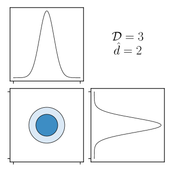
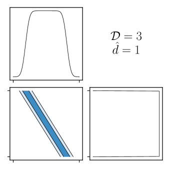
As a concrete example, consider the two posteriors illustrated in Fig. 1. In this case, both distributions have the same Kullback-Leibler divergence, but give very different parameter constraints. For the first distribution, both parameters are well constrained. In the second distribution, the one-dimensional marginal distributions show that the first parameter is slightly constrained, whilst the second parameter is completely unconstrained and identical to the prior. The full two-dimensional distribution tells a different story, showing that both parameters are heavily correlated, and that there is a strong constraint on a specific combination of parameters. In reality this is therefore a one-dimensional constraint that has been garbled across two parameters.

For the two-dimensional case in Fig. 1 we can by eye determine the number of constrained parameters, but in practical cosmological situations this is not possible. The cosmological parameter space of $\Lambda$CDM is six- (arguably seven-)dimensional Scott (2018), and modern likelihoods introduce a host of nuisance parameters to combat the influence of foregrounds and systematics. For example the Planck likelihood Planck Collaboration (2016) is in total 21-dimensional, the DES likelihood DES Collaboration (2017) is 26-dimensional, and their combination 41-dimensional (Tab. 1). Whilst samples from the posterior distribution represent a near lossless compression of the information present in this distribution, it goes without saying that visualising a 40-dimensional object is challenging. Triangle/corner plots Foreman-Mackey (2016) represent marginalised views of this information and can hide hidden correlations and constraints between three or more parameters. The fear is that one could misdiagnose a dataset that has powerful constraints if Fig. 1 occurred in higher dimensions. It would be helpful if there were a number $d$ similar to the Kullback-Leibler divergence $\mathcal{D}$ which quantifies the effective number of constrained parameters.

To this end, Spiegelhalter et al. (2002, ) introduced the Bayesian model complexity, defined as

$$\frac{\hat{d}}{2} =\log\frac{P(\hat{\theta})}{\pi(\hat{\theta})}-\left\langle\log\frac{\mathcal{P}}{\pi}\right\rangle_{\mathcal{P}}$$

$$=\mathcal{I}(\hat{\theta})-\left\langle\mathcal{I}\right\rangle_{\mathcal{P}}$$ (6)

In this case, the model complexity measures the difference between the information at some point $\hat{\theta}$ and the average amount of information. It thus quantifies how much overconstraint there is at $\hat{\theta}$, or equivalently the degree of model complexity. This quantity been historically used in several cosmological analyses Kunz et al. (2006); Bridges et al. (2009); Handley and Lemos (2019); Raveri and Hu (2019).

There is a degree of arbitrariness in Eq. 6 via the choice of point estimator $\hat{\theta}$. Typical recommended choices include the posterior mean

$$\hat{\theta}_{\mathrm{m}}=\int\theta\mathcal{P}(\theta)\operatorname{d}\!{\theta}=\left\langle\theta\right\rangle_{\mathcal{P},}$$ (7)

the posterior mode

$$\hat{\theta}_{\mathrm{mp}}=\max_{\theta}\mathcal{P}(\theta)$$ (8)

or the maximum likelihood point

$$\hat{\theta}_{\mathrm{ml}}=\max_{\theta}\mathcal{L}(\theta)=\max_{\theta}\mathcal{I}(\theta).$$ (9)

For the multivariate Gaussian case, $\hat{d}$ coincides with the actual dimensionality $d$ for all three of these estimators.

Unlike the Kullback-Leibler divergence, the BMC is only weakly prior dependent, since the evidence contributions in Eq. 6 cancel

$$\hat{d}=2\log\mathcal{L}(\hat{\theta})-\left\langle 2\log\mathcal{L}\right\rangle_{\mathcal{P}}.$$ (10)

The model dimensionality thus only changes with prior $\pi$ if the posterior bulk is significantly altered by changing the prior. For example $\hat{d}$ does not change if one merely expands the widths of a uniform prior that encompasses the posterior (in contrast to the evidence and Kullback-Leibler divergence).

Finally, the model complexity in Eq. 6 has the advantage of an information-theoretic backing and, like the Shannon information and Kullback-Leibler divergence, is additive for independent parameters.

II.5 The problem with principle component analysis

Intuitively from Fig. 1 one might describe the distribution as having one “component” that is well constrained, and another component for which the posterior provides no information.

The approach that is then followed by many researchers is to perform a principle component analysis (PCA), which proceeds thus

1. Compute the posterior covariance matrix

   $$\Sigma=\left\langle(\theta-\bar{\theta})(\theta-\bar{\theta})^{T}\right\rangle_{\mathcal{P}},\qquad\bar{\theta}=\left\langle\theta\right\rangle_{\mathcal{P}}$$ (11)

2. Compute the real eigenvalues $\lambda^{(i)}$ and eigenvectors $\Theta^{(i)}$ of $\Sigma$, defined via the equation

   $$\Sigma\Theta^{(i)}=\lambda^{(i)}\Theta^{(i)}$$ (12)

3. The eigenvectors with the smallest eigenvalues are the best constrained components, whilst the eigenvectors with large eigenvalues are poorly constrained.

One could therefore define an alternative to Eq. 6 based on the number of small eigenvalues, although this itself would depend on the eigenvalue cutoff used to define “unconstrained”.

Principle component analysis has intuitive appeal due in large part to the weight given to eigenvectors and eigenvalues early in a physicist’s undergraduate mathematical education. However, in many contexts that PCA is applied, the procedure is invalid almost to the point of nonsense.

The issue arises from the fact that the PCA procedure is not invariant under linear transformations. Typically the vectors $\theta$ have components with differing dimensionalities, in which case (12) is dimensionally invalid. Equivalently, changing the units that the axes are measured in changes both the eigenvalues and eigenvectors.

For example, for CosmoMC the default cosmological parameter vector is

$$\theta_{\mathrm{cosmo}}=(\Omega_{c}h^{2},\Omega_{b}h^{2},100\theta_{MC},\tau,\log 10^{10}A_{s},n_{s})$$ (13)

the first and second components have dimensions of $10^{-4}\mathrm{km}^{2}\mathrm{s}^{-2}\mathrm{Mpc}^{-2}$, the third is measured in units of $10^{-2}$ radians, whilst the final three are dimensionless. If one were to choose a different unit/scale for any one of these (somewhat arbitrary) dimensionalities, the eigenvalues and eigenvectors would change. To be clear, if all parameters are measured in the same units (as is the case for a traditional normal mode analysis) then PCA is a valid procedure.

Given these observations, the real question is not “is PCA the best procedure?”, but in fact “why does PCA usually work at all?” The answer to this question, and an information-theoretically valid PCA will be developed in an upcoming paper.

There are two ways in which one could adjust the naive PCA procedure to be dimensionally valid. The first is simply to normalise all inputs by the prior, say by computing the prior covariance matrix

$$\Sigma_{0}=\left\langle(\theta-\bar{\theta})(\theta-\bar{\theta})^{T}\right\rangle_{\pi},\qquad\bar{\theta}=\left\langle\theta\right\rangle_{\pi}$$ (14)

and then performing posterior PCA in a space normalised in some sense by this prior.

The second dimensionally valid approach would be to apply the PCA procedure to $\log\theta$. There is an implicit scale that one has to divide each component by in order to apply a logarithm, but this choice only alters the transformation by an additive constant, which PCA is in fact insensitive to. This amounts to finding components that are multiplicative combinations of parameters. A good example of such a combination is $\Omega_{b}h^{2}$, or $S_{8}=\sigma_{8}\sqrt{\Omega_{m}/0.3}$, indicating that physicists are used to thinking in these terms.

II.6 The anatomy of a Gaussian

Figure 2: The typical set of a $d$-dimensional Gaussian distribution can be visualised by plotting the posterior probability distribution of the Shannon information $\mathcal{I}$. The posterior has mean $\mathcal{D}$ and variance $\frac{d}{2}$. The posterior maximum occurs at $\mathcal{I}=\mathcal{D}+1$, and the domain is $(-\infty,\mathcal{I}_{\max}]$. The above plot is shown for $d=16$ in analogy with the Planck likelihood from Fig. 8 and Tab. 3.

As a concrete example of all of the above ideas, we will consider them in the context of a $d$-dimensional multivariate Gaussian. Consider a posterior $\mathcal{P}$, with parameter covariance matrix $\Sigma$ and mean $\mu$, arising from a uniform prior $\pi$ with volume $V$ which fully encompasses the posterior. It is easy to show that the Kullback-Leibler divergence for such a distribution is

$$\mathcal{D}=\log\frac{V}{\sqrt{|2\pi e\Sigma|}}$$ (15)

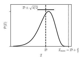
Each iso-posterior ellipsoidal contour $\mathcal{P}(\theta)=\mathcal{P}$ defines a Shannon information $\mathcal{I}=\log\mathcal{P}/\pi$. The posterior distribution $\mathcal{P}(\theta)$ induces an offset, re-scaled, $\chi^{2}_{d}$ distribution on the Shannon information

$$\mathcal{P}(\mathcal{I}) =\frac{1}{\Gamma(d/2)}e^{\mathcal{I}-\mathcal{I}_{\max}}{(\mathcal{I}_{\max}-\mathcal{I})}^{\frac{d}{2}-1},$$ (16)

$$\mathcal{I}_{\max} =\log\frac{V}{\sqrt{|2\pi\Sigma|}}=\mathcal{D}+\frac{d}{2},$$ (17)

$$\mathcal{I} \in(-\infty,\mathcal{I}_{\max}],\qquad\mathcal{I}\approx\mathcal{D}\pm\sqrt{d/2},$$ (18)

which may be seen graphically in Fig. 2. This distribution has mean $\mathcal{D}$ by the definition of the Kullback-Leibler divergence, and standard deviation $\sqrt{d/2}$. The region for which the distribution $\mathcal{P}(\mathcal{I})$ is significantly non-zero defines the typical set of the posterior, indicating the Shannon information of points that would be typically drawn from the distribution $\mathcal{P}$. For this Gaussian case, the maximum posterior $\hat{\theta}_{\mathrm{mp}}$, likelihood $\hat{\theta}_{\mathrm{ml}}$ and mean $\hat{\theta}_{\mathrm{m}}$ parameter points coincide, and have Shannon information $I_{\max}=\mathcal{D}+\frac{d}{2}$.

III Bayesian model dimensionality

Figure 3: Bayesian dimensionality for the common one-dimensional distributions in Tab. 2. Widths are normalised so that the distributions all have the same Kullback-Leibler divergence $\mathcal{D}$. The dashed curve in all plots is a Gaussian distribution.

III.1 The problem with Bayesian model complexity $\hat{d}$

Whilst the BMC is widely used in the statistical literature, and recovers the correct answer in the case that the posterior distribution is Gaussian, there are three key problems that should be noted.

First, it is clear that the arbitrariness regarding the choice of estimator is far from ideal, and as we shall show in Sec. IV differing choices yield distinct and contradictory answers. A proper information theoretic quantity should be unambiguous.

Second, and most importantly in our view, estimators are not typical posterior points. In general, point estimators such as the maximum likelihood, posterior mode or mean have little statistical meaning in a Bayesian sense, since they occupy a region of vanishing posterior mass. This can be seen in Fig. 2, which shows that whilst an estimator may represent a point of high information, it lies in a zero posterior mass region — If $d>2$, one can see from Eq. 16 that $\mathcal{P}(\mathcal{I}_{\max})=0$. A physical example familiar to undergraduate quantum physicists is that of the probability distribution of an electron in a 1s orbital: The most likely location to find an electron is the origin, whilst the radial distribution function shows that the most likely region to find an electron is at the Bohr radius $a_{0}$.

A practical consequence of these observations is that if you choose the highest likelihood point from an MCMC chain, it will lie at a likelihood some way below the true maximum, and in general one should not expect points in the MCMC chain to lie close to the mean, mode or maximum likelihood point in likelihood space. In general, to compute these point estimators an additional calculation must be performed such as a explicit posterior and likelihood maximisation routines or a mean and likelihood computation.

Third most estimators are parameterisation dependent. Namely, if one were to transform the variables and distribution to a different coordinate system via

$$\theta \to\tilde{\theta}=f(\theta),$$ (19)

$$\mathcal{P}(\theta) \to\tilde{\mathcal{P}}(\tilde{\theta})=\mathcal{P}(f^{-1}(\tilde{\theta}))|{\partial\theta}/{\partial\tilde{\theta}}|,$$ (20)

$$\pi(\theta) \to\tilde{\pi}(\tilde{\theta})=\pi(f^{-1}(\tilde{\theta}))|{\partial\theta}/{\partial\tilde{\theta}}|,$$ (21)

then neither the posterior mean from Eq. 7 nor the posterior mode from Eq. 8 transform under Eq. 19 if the transformation $f$ is non-linear (i.e. the Jacobian $|\partial\theta/\partial\tilde{\theta}|$ depends on $\tilde{\theta}$). It should be noted that this parameterisation variance is not quite as bad as it is for the PCA case, which is dependent on even linear transformations of the parameter vector. The maximum likelihood point from Eq. 9 does correctly transform, since the Jacobian terms in Eqs. 20 and 21 cancel in the Shannon information. Parameterisation dependency is a highly undesirable ambiguity, particularly in the context of cosmology where in general the preferred choice of parameterisation varies between likelihoods and sampling codes Zuntz et al. (2015); Lewis and Bridle (2002); Audren et al. (2013).

Finally, specifically to the mean estimator, for some cosmological likelihoods there may be no guarantee that the mean even lies in the posterior mass, for example in the $\sigma_{8}$-$\Omega_{m}$ banana distribution visualised by KiDS van Uitert et al. (2018). In cosmology, we do not necessarily have the luxury of Gaussianity or convexity.

III.2 The Bayesian model dimensionality $\tilde{d}$

Considering Fig. 2, the fundamental concept to draw is that the BMC leverages the fact that the difference between the Shannon information $\mathcal{I}$ at the posterior peak and the mean of the posterior bulk is $d/2$ for the Gaussian case.

However, there is a second way of bringing the dimensionality out of Fig. 2 via the variance of the posterior bulk. With this in mind, we define the Bayesian model dimensionality as

$$\frac{\tilde{d}}{2} =\int\mathcal{P}(\theta){\left(\log\frac{\mathcal{P}(\theta)}{\pi(\theta)}-\mathcal{D}\right)}^{2}\operatorname{d}\!{\theta},$$ (22)

$$=\left\langle{\mathcal{I}}^{2}\right\rangle_{\mathcal{P}}-{\left\langle\mathcal{I}\right\rangle}_{\mathcal{P}}^{2}.$$ (23)

or equivalently as

$$\tilde{d}/2=\left\langle{\left(\log\mathcal{L}\right)}^{2}\right\rangle_{\mathcal{P}}-{\left\langle\log\mathcal{L}\right\rangle}^{2}_{\mathcal{P}}.$$ (24)

We note that this form for quantifying model dimensionality is discussed in passing by Gelman et al. (2004, p 173) and Spiegelhalter et al. , who conclude that $\tilde{d}$ is less numerically stable than $\hat{d}$. As we shall discuss in Sec. IV we find that when applied to cosmological likelihoods the opposite is in fact true. This measure of model dimensionality is also discussed briefly in the landmark nested sampling paper by Skilling (2006), by Raveri and Hu (2019), in a cosmological context in terms of $\chi^{2}$ in Kunz et al. (2006) and Liddle (2007); and was used as part of the Planck analysis Planck Collaboration (2018).

The definition of $\tilde{d}$ shares all of the desiderata that $\hat{d}$ provides, namely both $\tilde{d}$ and $\hat{d}$ are weakly prior dependent, additive for independent parameters and recover the correct answer in the Gaussian case. We believe that there are several attractive theoretical characteristics of $\tilde{d}$ that we view as advantages over $\hat{d}$

First, $\tilde{d}$ relies only on points drawn from the typical set, which is highly attractive from a Bayesian and information theoretic point of view, and more consistent when used alongside a traditional MCMC analysis of cosmological posteriors.

Second, there is a satisfying progression in the fact that whilst the mean of the Shannon information $\mathcal{D}$ gives one an overall constraint, the next order statistic (the variance) yields a measure of the dimensionality of the constraint.

Finally, in eschewing estimators this measure is completely unambiguous, as it removes all arbitrariness associated with both estimator and underlying parameterisation choice.

It should be noted that the computation of $\mathcal{D}$ requires nested sampling to provide an estimate of $\log\mathcal{Z}$. The dimensionality $\tilde{d}$ on the other hand can be computed from a more traditional MCMC chain via Eq. 24.

III.3 Thermodynamic interpretation

There is a second motivation for the BMD arising from a thermodynamic viewpoint. The thermodynamic generalisation of Bayes theorem is

$$\mathcal{L}^{\beta}(\theta)\times\pi(\theta) =\mathcal{P}_{\beta}(\theta)\times\mathcal{Z}(\beta),$$ (25)

$$\mathcal{Z}(\beta) =\int\mathcal{L}^{\beta}(\theta)\pi(\theta)\operatorname{d}\!{\theta},$$ (26)

where on the left-hand side of Eq. 25, the inverse-temperature $\beta=\frac{1}{T}$ raises the likelihood $\mathcal{L}$ to the power of $\beta$ and on the right-hand side the posterior has a non-trivial dependency on temperature, denoted by a subscript $\beta$. When the evidence in Eqs. 25 and 26 is a function of $\beta$ it is usually called the partition function.

The link to thermodynamics comes by considering $\theta$ to be a continuous index $i$ over microstates, the negative log-likelihood to be the energy $E$ of a microstate, and the prior to be the degeneracy of microstates $g$

$$i\leftrightarrow\theta\qquad E_{i}\leftrightarrow-\log\mathcal{L}(\theta)\qquad g_{i}\leftrightarrow\pi(\theta),$$

$$g_{i}e^{-\beta E_{i}}\leftrightarrow\mathcal{L}(\theta)^{\beta}\pi(\theta).$$ (27)

It should be noted that one of the principal advantages of nested sampling is that (other than the stopping criterion) it is blind to $\beta$, and therefore samples at all temperatures simultaneously. Nested samplers are best described as partition function calculators rather than as posterior samplers. This will be explored in further detail in an upcoming paper Handley et al. (2019).

In its thermodynamic form, the evidence becomes a generating function Wilf (2006)

$$\frac{\operatorname{d}\!{}^{2}}{\operatorname{d}\!{\beta}^{2}}\log\mathcal{Z}(\beta) =\frac{\operatorname{d}\!{}}{\operatorname{d}\!{\beta}}\left\langle\log\mathcal{L}\right\rangle_{\mathcal{P}_{\mathcal{\beta}}}=\frac{\tilde{d}}{2},$$ (28)

and we may identify the BMD as being related to the rate of change of average loglikelihood(energy) with inverse temperature. The BMD is therefore proportional to the Bayesian analogue of a heat capacity, $C=\frac{\operatorname{d}\!{}}{\operatorname{d}\!{T}}\langle E\rangle=\beta^{2}\frac{\operatorname{d}\!{}}{\operatorname{d}\!{\beta}}\langle-E\rangle$ and, like all heat capacities, is proportional to system size, or equivalently to the number of active degrees of freedom (i.e. dimensions).

III.4 Analytical examples

	$\mathcal{P}^{\ast}$	$\exp(\mathcal{D}^{\ast})$	$\tilde{d}$	$\hat{d}$
Gaussian	$e^{-x^{2}/2}$	${1/\sqrt{2\pi e}}$	$1$	1
Top-hat	$x\in[-1,1]$	${1}$	$0$	$0$
Triangle	$1-|x|$	${1/\sqrt{e}}$	$1/2$	$1$
Cosine	$\cos^{2}x$	${e/2\pi}$	$\frac{2(\pi^{2}-9)}{3}\approx 0.58$	$\log\frac{2^{4}}{e^{2}}\approx 0.77$
Logistic	$\frac{e^{-x}}{{(1+e^{-x})}^{2}}$	${1/e^{2}}$	$\frac{24-2\pi^{2}}{3}\approx 1.42$	$\log\frac{e^{4}}{2^{4}}\approx 1.33$
Laplace	$e^{-|x|}$	${1/2e}$	$2$	$2$
Cauchy	${(1+x^{2})}^{-1}$	${1/4\pi}$	$\frac{2\pi^{2}}{3}\approx 6.58$	$\log 2^{4}\approx 2.77$

Table 2: Dimensionalities for one dimensional analytic distributions. The first column indicates the unnormalised probability density $\mathcal{P}^{\ast}(x)$. An arbitrary width $\sigma$ can be added by remapping $\mathcal{P}^{\ast}(x)\to\frac{1}{\sigma}\mathcal{P}^{\ast}(x/\sigma)$. The second column indicates the unnormalised Kullback-Leibler divergence $\mathcal{D}^{\ast}=\mathcal{D}-\log V/\sigma$ where the implicit prior is taken to encompass the posterior mass with width $V\gg\sigma$. The final two columns show the BMDs and BMCs respectively, which are independent of both $V$ and $\sigma$. As expected, the Gaussian has dimensionality $\tilde{d}=\hat{d}=1$, shorter and fatter distributions have lower dimensionalities, whilst narrower and taller dimensionalities have dimensions greater than one. This effect can be seen graphically in Fig. 3.

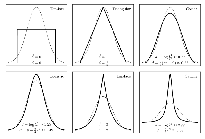
We apply the BMD from Eq. 23 and the BMC from Eq. 6 to six additional univariate analytical examples: Top-hat, Triangular, Cosine, Logistic, Laplace and Cauchy. The analytical forms for the probability distribution, Kullback-Leibler divergence, BMD and BMC are listed in Tab. 2, and plotted in Fig. 3. In all cases, we assume a uniform prior of volume $V$ which fully encompasses the posterior.

We find that whilst the Gaussian distribution gives $\tilde{d}=1$, distributions that are shorter and fatter give $\tilde{d}<1$, whilst distributions that are narrower and taller give $\tilde{d}>1$. Both measures of $\tilde{d}$ and $\hat{d}$ are in broad agreement. The Top-Hat (dimensionality $0$) and Cauchy distributions (dimensionality $\gg 1$) represent pathological cases at either end of the scale, while the remainder all give dimensionalities of order $1$. In general, $\hat{d}$ is closer to unity than $\tilde{d}$, on account of the “numerical stability” quoted by Gelman et al. (2004). However, accurate computation of $\hat{d}$ is predicated on an exact computation of the maximum, which (as shown in Sec. IV) becomes increasingly unstable in higher dimensions and in cosmological applications.

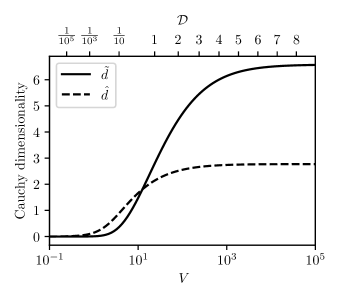
It should also be noted that whilst the Cauchy distribution gives a very high dimensionality when integrated over its full infinite domain, if the domain is restricted by the prior then the dimensionality drops to more sensible values (Fig. 4).

Figure 4: Dependency of dimensionality and Kullback-Leibler divergence on prior volume for a Cauchy distribution $\mathcal{P}(x)\propto(1+x^{2})^{-1}$. Whilst the BMD and BMC are pathologically large $(\gg 1)$ if the full domain of the Cauchy distribution is included, truncating the range to a lower prior volume $x\in[-V/2,V/2]$ reduces the dimensionality to more sensible values.

III.5 Applications

BMDs can be used in a variety of statistical analyses. In this subsection we review a few of the possibilities.

III.5.1 The number of constrained cosmological parameters

As detailed in Tab. 1, cosmological likelihoods typically introduce a large number of nuisance parameters in addition to cosmological ones, and they typically constrain a non-trivial combination of parameters. If one has datasets $A$ and $B$, one can compute the individual model dimensionalities $\tilde{d}_{A}$ and $\tilde{d}_{B}$, as well as the model dimensionality of using both datasets together $\tilde{d}_{AB}$. Computing the crossover of these dimensionalities for any choice of $d$, $\tilde{d}$ or $\hat{d}$

$$\tilde{d}_{A\cap B}=\tilde{d}_{A}+\tilde{d}_{B}-\tilde{d}_{AB}$$ (29)

will give the (effective) number of constrained cosmological parameters shared between the datasets, since any parameters constrained by just one of the datasets subtract out of the above expression. This quantity forms a cornerstone of part of the tension analysis in Handley and Lemos (2019), and cosmological examples can be seen in the lower section of Tab. 3.

III.5.2 Penalising the number of model parameters

Bayesian evidences are traditionally used in model comparison via Bayes theorem for models

$$P(\mathcal{M}_{i})=\frac{P(D|\mathcal{M}_{i})P(\mathcal{M}_{i})}{\sum_{j}P(D|\mathcal{M}_{i})P(\mathcal{M}_{j})}=\frac{\mathcal{Z}_{i}\Pi_{i}}{\sum_{j}\mathcal{Z}_{j}\Pi_{j}},$$ (30)

where $\Pi_{i}=P(\mathcal{M}_{i})$ are the model priors, which are typically taken to be uniform. Often the data may not be discriminative enough to pick an unambiguously best model via the model posteriors. The correct Bayesian approach in this case is to perform model marginalisation over any future predictions Gariazzo and Mena (2019). However, in other works Martin et al. (2016); Collaboration (2018) the Kullback-Leibler divergence has been used to split this degeneracy. The strong prior dependency of the KL divergence can make this a somewhat unfair choice for splitting this degeneracy, and users may find that the model dimensionality is a fairer choice

One implementation of this approach would be to apply a post-hoc model prior of

$$\Pi_{i}(\lambda)=\lambda e^{-\lambda\tilde{d}_{i}}$$ (31)

using for example $\lambda=1$. This amounts to a logarithmic Bayes factor between models of

$$\log\mathcal{B}_{j}^{i}=(\log\mathcal{Z}_{i}-\lambda\tilde{d}_{i})-(\log\mathcal{Z}_{j}-\lambda\tilde{d}_{j})$$ (32)

This approach is not strictly Bayesian, since $\tilde{d}_{i}$ is computed from the data and $\Pi_{i}(\lambda)$ is therefore not a true prior. However readers familiar with the concepts of sparse reconstructions Higson et al. (2019) will recognise the parallels between sparsity and this approach, as one is effectively imposing a penalty factor that promotes models that use as few parameters as necessary to constrain the data.

III.5.3 Information criteria

Whilst the authors’ preferred method of model comparison is via the Bayesian evidence, other criteria have been used in the context of cosmology Liddle (2004, 2007): The Akaike information criterion (AIC) Akaike (1974) and Bayesian information criterion (BIC) Schwarz (1978) are defined respectively via

$$\mathrm{AIC} =-2\log\mathcal{L}_{\max}+2k,$$ (33)

$$\mathrm{BIC} =-2\log\mathcal{L}_{\max}+k\ln N,$$ (34)

where $k$ is the number of parameters in the model and $N$ is the number of datapoints used in the fit. These criteria could be modified in a Bayesian sense by replacing $k$ with the BMD $\tilde{d}$. A similar modification has been discussed in the context of the deviance information criterion (DIC) Liddle (2007); Kunz et al. (2006).

IV Numerical examples

Dataset	$\hfill\mathcal{D}_{\phantom{m}}\hfill$	$\hfill\tilde{d}_{\phantom{m}}\hfill$	$\hfill\hat{d}_{\mathrm{m}}\hfill$	$\hfill\hat{d}_{\mathrm{mp}}\hfill$	$\hfill\hat{d}_{\mathrm{ml}}\hfill$	$d$
S$H_{0}$ES	$2.52\pm 0.03$	$0.93\pm 0.03$	$-40.12\pm 0.02$	$0.96\pm 0.02$	$0.96\pm 0.02$	$6$
BOSS	$5.06\pm 0.05$	$2.95\pm 0.07$	$-9.55\pm 0.05$	$2.93\pm 0.05$	$2.93\pm 0.05$	$6$
DES	$22.82\pm 0.15$	$14.03\pm 0.30$	$10.79\pm 0.14$	$14.45\pm 0.14$	$17.85\pm 0.14$	$26$
Planck	$44.48\pm 0.20$	$15.84\pm 0.38$	$14.91\pm 0.16$	$15.68\pm 0.16$	$18.91\pm 0.16$	$21$
S$H_{0}$ES+Planck	$45.02\pm 0.20$	$15.97\pm 0.36$	$14.64\pm 0.15$	$15.39\pm 0.15$	$18.40\pm 0.15$	$21$
BOSS+Planck	$43.36\pm 0.20$	$15.89\pm 0.38$	$15.11\pm 0.17$	$15.57\pm 0.17$	$18.89\pm 0.17$	$21$
DES+Planck	$61.13\pm 0.25$	$25.88\pm 0.62$	$20.79\pm 0.25$	$23.54\pm 0.25$	$29.30\pm 0.25$	$41$
S$H_{0}$ES$\cap$Planck	$1.99\pm 0.29$	$0.80\pm 0.52$	$-39.84\pm 0.23$	$1.25\pm 0.23$	$1.48\pm 0.23$	$6$
BOSS$\cap$Planck	$6.18\pm 0.30$	$2.91\pm 0.54$	$-9.75\pm 0.23$	$3.04\pm 0.23$	$2.96\pm 0.23$	$6$
DES$\cap$Planck	$6.17\pm 0.36$	$3.98\pm 0.77$	$4.91\pm 0.32$	$6.59\pm 0.32$	$7.46\pm 0.32$	$6$

Table 3: Bayesian model dimensionalities for cosmological datasets. The first column indicates the Kullback-Leibler divergence $\mathcal{D}$ from Eq. 5, and the second column shows the Bayesian model dimensionality $\tilde{d}$ from Eq. 23. The remaining three columns show the Bayesian model complexity $\hat{d}$ from Eq. 6 with the estimator chosen as the posterior mean, posterior mode and maximum likelihood point respectively. The final three rows show the intersection statistics, computed using the equivalents of Eq. 29.

Figure 5: Cosmological parameters unconstrained by DES. Whilst DES provides constraints on four of the cosmological parameters, it tells us nothing of $\tau$, and little of a correlated combination of $\ln 10^{10}A_{s}$ and $n_{s}$. This figure should be compared with Fig. 1.

Figure 6: One-dimensional marginalised default prior (black) and Planck posterior (red). The Bayesian model dimensionality of $\tilde{d}_{\textit{Planck}}\approx 16$ is reflected by the fact that only a subset of the nuisance parameters are constrained by the data.

Figure 7: One-dimensional marginalised default prior (black) and DES Y1 posterior (red). The Bayesian model dimensionality of $\tilde{d}_{\mathrm{DES}}\approx 14$ is reflected by the fact that only a combination of the cosmological parameters and a subset of the nuisance parameters are constrained by the data.

Figure 8: Shannon information for the numerical examples considered in this paper. These plots are laid out in the same manner as Fig. 2, with the mean of each distribution representing the Kullback-Leibler divergence, and the variance the Bayesian model dimensionality. The main difference between these plots and Fig. 2 is that the posterior mean $\mathcal{I}_{\mathrm{m}}$, mode $\mathcal{I}_{\mathrm{mp}}$ and maximum likelihood $\mathcal{I}_{\mathrm{ml}}$ points no longer coincide on account of the non-uniform priors and non-trivial parameterisation involved in cosmological modelling. The multiple curves for $\mathcal{P}(\mathcal{I})$ represent independent samples from the distribution of nested sampling prior volumes used to compute the Shannon information, and the spread in these curves accounts for the errors in estimating the quantities detailed in Tab. 3.

Figure 9: Marginalised posterior likelihoods (in black), maximum likelihood points (ML, in blue), maximum posterior points (MP, in red) and means (in green), for some of the numerical examples used in this paper. The top plots detail the one-dimensional marginalised posterior on the Hubble parameter, whilst the lower plots show the two-dimensional marginalised posterior on $\sigma_{8}$ and $\Omega_{m}$. Top left shows the S$H_{0}$ES likelihood, top center Planck, and top right the combination of both. Bottom left shows the DES posterior, bottom center Planck, and bottom right their combination.

IV.1 Cosmological likelihoods

We test our method on real data by quantifying the effective number of constrained parameters in four publicly available cosmological datasets, assuming a six-parameter $\Lambda$CDM cosmological model. We use the following six sampling parameters to describe this model: The density of baryonic matter $\Omega_{b}h^{2}$, the density of cold dark matter $\Omega_{c}h^{2}$, $\theta_{MC}$ an approximation of the ratio of the sound horizon to the angular diameter distance at recombination, the optical depth to reionisation $\tau$ and the amplitude and tilt of the primordial power spectrum $A_{s}$ and $n_{s}$. This is the default parameterisation for CosmoMC Lewis and Bridle (2002), and is chosen to maximize the efficiency of Metropolis-Hastings sampling codes for CMB data. The possible effects of this parameterisation choice in non-CMB constraints will be explored in future work.

We use four key datasets in our analysis. First, we use measurements of temperature and polarization anisotropies in the CMB measured by Planck in the form of the publicly available Planck 2015 data Planck Collaboration (2016). Second, we use local cosmic distance ladder measurements of the expansion rate, using type Ia SNe calibrated by variable Cepheid stars, and implemented as a gaussian likelihood with mean and standard deviation given by the latest results obtained by the S$H_{0}$ES collaboration Riess et al. (2018). Third, we use the Dark Energy Survey (DES) Year 1 combined analysis of cosmic shear, galaxy clustering and galaxy-galaxy lensing (a combination commonly referred to as ‘3x2’) DES Collaboration (2017). Finally, we use Baryon Acoustic Oscillation (BAO) measurements from the Baryon Oscillation Spectroscopic Survey (BOSS) DR12 Alam and et al. (2017); Beutler et al. (2011); Ross et al. (2015). The number of parameters that we sample over for each likelihood is described in Tab. 1

IV.2 Nested sampling

To compute the log-evidence $\log\mathcal{Z}$, Kullback-Leibler divergence $\mathcal{D}$ and Bayesian model dimensionality $\tilde{d}$, we use the outputs of a nested sampling run produced by CosmoChord Handley (2019); Lewis and Bridle (2002); Handley et al. (2015a, b); Lewis (2013) and the equations

$$\mathcal{Z}\approx \sum_{i=1}^{N}\mathcal{L}_{i}\times\frac{1}{2}(X_{i-1}-X_{i+1}),$$

$$\mathcal{D}\approx \sum_{i=1}^{N}\frac{\mathcal{L}_{i}}{\mathcal{Z}}\log\frac{\mathcal{L}_{i}}{\mathcal{Z}}\times\frac{1}{2}(X_{i-1}-X_{i+1}),$$

$$\frac{\tilde{d}}{2}\approx \sum_{i=1}^{N}{\frac{\mathcal{L}_{i}}{\mathcal{Z}}\left(\log\frac{\mathcal{L}_{i}}{\mathcal{Z}}-\mathcal{D}\right)}^{2}\times\frac{1}{2}(X_{i-1}-X_{i+1}),$$

$$X_{i}= t_{i}X_{i-1},\qquad X_{0}=1,\qquad X_{N+1}=0,$$

$$P(t_{i}) =n_{i}t_{i}^{n_{i}-1}\>[0<t_{i}<1]$$ (35)

where $\mathcal{L}_{i}$ are the $N$ likelihood contours of the discarded points, $X_{i}$ are the prior volumes, $n_{i}$ are the number of live points and $t_{i}$ are real random variables. We compute $1000$ batches of the samples $\{t_{i}:i=1\ldots N\}$. Code for performing the above calculation is provided by the Python package anesthetic Handley (2019). For our final runs, we used the CosmoChord settings $n_{\mathrm{live}}=1000$, $n_{\mathrm{prior}}=10000$, with all other settings left at their defaults for CosmoChord version 1.15. For more detail, see Skilling (2006) or Handley and Lemos (2019).

In order to compute the maximum likelihood and posterior points, we found that the most reliable procedure was to use a Nelder-Mead simplex method Nelder and Mead (1965) with the initial simplex defined by the highest likelihood live points found before termination.

IV.3 Results

Our main results are detailed in Tab. 3, where we report the Bayesian model dimensionality $\tilde{d}$ obtained from Eq. 23, compared with the values obtained for the Bayesian model complexity using Eq. 6 using three different estimators from Eqs. 7, 8 and 9: the posterior mean, posterior mode and maximum likelihood. We use the four individual datasets described in Sec. IV.1, as well as in combination with Planck. We also report the shared dimensionalities from Eq. 29 using Planck as the common baseline in the bottom three rows of the table.

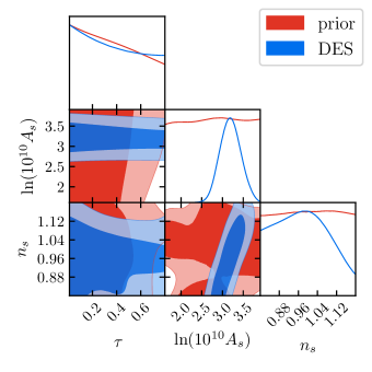
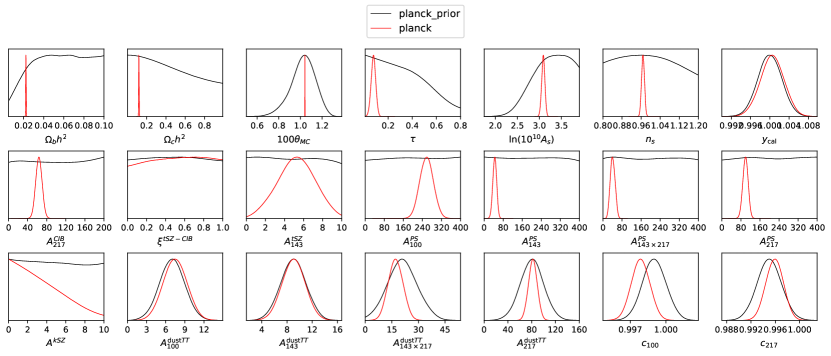
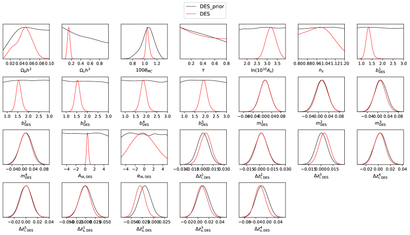
The BMDs produce sensible values in all cases. It should be noted that in general the BMDs are lower than the number of dimensions that are sampled over (Tab. 3): S$H_{0}$ES constrains only one parameter ($H_{0}$), BOSS constrains three ($\Omega_{b}h^{2}$,$\Omega_{c}h^{2}$ and a degenerate $H_{0}$-$A_{s}$ constraint), and DES and Planck constrain only some combinations of cosmological and nuisance parameters as shown by Figs. 5, 6 and 7.

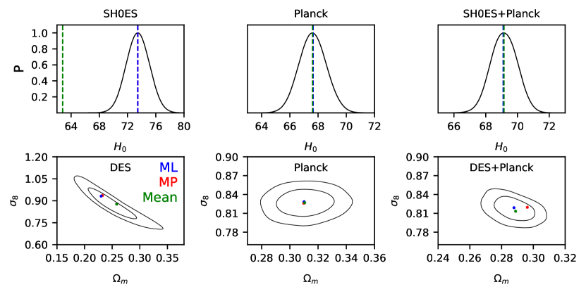
The shared dimensionalities also match cosmological intuition. For example, $\tilde{d}_{\mathrm{DES{}\cap\textit{Planck}{}}}$ shows that DES only constrains four cosmological parameters, as it provides no constraint on $\tau$, and only constrains a combination of $n_{s}$ and $\log 10^{10}A_{s}$. This is shown graphically in Fig. 5, which should be compared with Fig. 1.

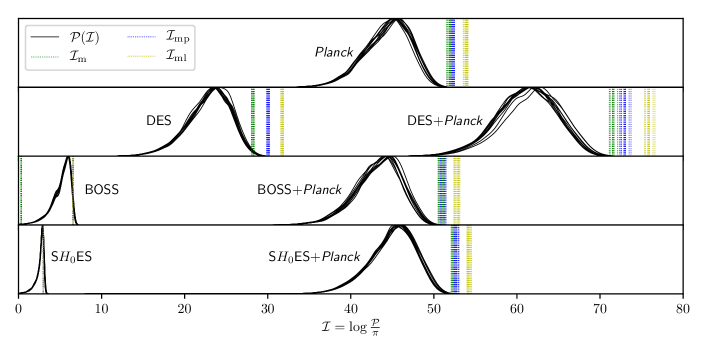
All error bars on the dimensionalities arise from nested sampling’s imperfect knowledge of prior volumes used to compute the posterior weights. It is likely that the error could be lowered by using a more traditional MCMC run Zuntz et al. (2015); Lewis and Bridle (2002); Audren et al. (2013), although care must be taken with the MCMC error estimation since marginalising over the likelihood is numerically more unstable than that of traditional expectation values. The process of computing the Bayesian model dimensionalities and their errors is visualised in Fig. 8, which should be compared with Fig. 2.

The results for Bayesian model complexities on the other hand are nowhere near as satisfactory. The arbitrariness in the choice of estimator can be seen clearly, and in general we find $\hat{d}_{\mathrm{m}}<\hat{d}_{\mathrm{mp}}<\hat{d}_{\mathrm{ml}}$. This variation in the choice of estimator is demonstrated graphically in Fig. 9. The two maximisation estimators come out a little high, with the most extreme example being that the maximum likelihood estimator claims that there are $7.5$ shared dimensions between DES and Planck, which is concerning given that there are only six parameters that are shared between them. The fact that the maximum likelihood estimator consistently produces dimensionalities that are too large is unfortunate, given that it is the best motivated of all three estimators.

The mean estimator on the other hand is generally a little lower than expected and produces nonsensical results for S$H_{0}$ES and BOSS alone, where as mentioned in Sec. III.1 the parameterisation variance of the estimator makes the mean extremely unreliable. In the case of S$H_{0}$ES, we are sampling over six cosmological parameters, but only constrain $H_{0}$, which is only one combination of those six. As a consequence, the value of $H_{0}$ derived from the means of the mostly unconstrained cosmological parameters is completely prior dominated.

The fact that Fig. 9 shows that the estimators are most consistent for Planck data is also very telling. This is not caused by any properties of the Planck data, instead it is a consequence of the parameterisation choice: All of these posteriors are obtained using the CosmoMC parameterisation, which is chosen to be optimal for CMB analyses. The parameters that other surveys like DES and S$H_{0}$ES constrain are obtained as derived parameters, which changes both the mean and the maximum posterior.

V Conclusion

In this paper we interpret the variance in the Shannon information as a measure of Bayesian model dimensionality and present it as an alternative to Bayesian model complexity currently used in the literature. We compared these two measures of dimensionality theoretically and in the context of cosmological parameter estimation, and found that the Bayesian model dimensionality proves more accurate in reproducing results consistent with intuition.

Whilst the Bayesian model dimensionality has been acknowledged in the literature in different forms, it has yet not been widely used in cosmology. Given the ease with which the Bayesian model dimensionality can be computed from MCMC chains, we hope that this work persuades cosmologists to use this crucial statistic as a part of their analyses. For those using Nested Sampling, we hope that in future the reporting of the triple of Evidence, Kullback-Leibler divergence and Bayesian model dimensionality $(\mathcal{Z},\mathcal{D},\tilde{d})$ becomes a scientific standard.