Single-trajectory spectral analysis of scaled Brownian motion

Abstract

A standard approach to study time-dependent stochastic processes is the power spectral density (PSD), an ensemble-averaged property defined as the Fourier transform of the autocorrelation function of the process in the asymptotic limit of long observation times, $T\to\infty$. In many experimental situations one is able to garner only relatively few stochastic time series of finite $T$, such that practically neither an ensemble average nor the asymptotic limit $T\to\infty$ can be achieved. To accommodate for a meaningful analysis of such finite-length data we here develop the framework of single-trajectory spectral analysis for one of the standard models of anomalous diffusion, scaled Brownian motion. We demonstrate that the frequency dependence of the single-trajectory PSD is exactly the same as for standard Brownian motion, which may lead one to the erroneous conclusion that the observed motion is normal-diffusive. However, a distinctive feature is shown to be provided by the explicit dependence on the measurement time $T$, and this ageing phenomenon can be used to deduce the anomalous diffusion exponent. We also compare our results to the single-trajectory PSD behaviour of another standard anomalous diffusion process, fractional Brownian motion, and work out the commonalities and differences. Our results represent an important step in establishing single-trajectory PSDs as an alternative (or complement) to analyses based on the time-averaged mean squared displacement.

17th March 2024

1 Introduction

The spectral analysis of measured position time series ("trajectories") $X(t)$ of a stochastic process provides important insight into its short and long time behaviour, and also unveils its temporal correlations [1]. In standard textbook settings, spectral analyses are carried out by determining the so-called power spectral density (PSD) $\mu(f)$ of the process. The PSD is classically calculated by first performing a Fourier transform of an individual trajectory $X(t)$ over the finite observation time $T$,

$$S(f,T)=\frac{1}{T}\left|\int_{0}^{T}e^{ift}X(t)dt\right|^{2},$$ (1)

where $f$ denotes the frequency. The quantity $S(f,T)$ for finite observation times $T$ is, of course, a random variable. The standard PSD yields from $S(f,T)$ by averaging it over a statistical ensemble of all possible trajectories. After taking the asymptotic limit $T\to\infty$, one obtains the standard PSD

$$\mu(f)=\lim_{T\to\infty}\frac{1}{T}\left\langle\left|\int_{0}^{T}e^{ift}X(t)dt\right|^{2}\right\rangle,$$ (2)

where the angular brackets denote the statistical averaging.

Following this definition, the standard PSD was determined for various processes across many disciplines. This includes, for instance, the variation of the loudness of musical performances [2], the temporal evolution of climate data [3] and of the waiting-times between earthquakes [4], the retention times of chemical tracers in groundwater [5] and noises in graphene devices [6], fluorescence intermittency in nano-devices [7], current fluctuations in nanoscale electrodes [8], or ionic currents across nanopores [9]. The PSD was also calculated analytically for individual time series in a stochastic model describing blinking quantum dots [10], for non-stationary processes taking advantage of a generalised Wiener-Khinchin theorem [11, 12], for the process of fractional Brownian motion with random reset [13], the running maximum of a Brownian motion [14], as well as for diffusion in strongly disordered Sinai-type systems [15], to name but a few stray examples.

An alternative approach geared towards realistic experimental situations was recently proposed—based directly on the finite-time, single-trajectory PSD (1) [16, 17] (see also [18]). The need for such an alternative to the standard PSD (2) is two-fold. First, while the asymptotic limit $T\to\infty$ can well be taken in mathematical expressions, it cannot be realistically achieved experimentally. This especially holds for typical, modern single particle tracking experiments, in which the observation time is limited by the microscope’s focus or the fluorescence lifetime of the dye label tagging the moving particle of interest [19]. In general, apart from the dependence on the frequency $f$ the single-trajectory PSD (1) therefore explicitly is a function of the observation time $T$. Moreover, fluctuations between individual results $S(f,T)$ of the single-trajectory PSD will be observed, even for normal Brownian motion [16]. Second, and maybe even more importantly, while such fluctuations between trajectories may, of course, be mitigated by taking an average over a statistical ensemble, in many cases the number of measured trajectories is too small for a meaningful statistical averaging. Indeed, for the data garnered in, for instance, in vivo experiments [19], climate evolution [20], or the evolution of financial markets [21] one necessarily deals with a single or just a few realisations of the process. As we will show, despite the fluctuations between individual trajectories relevant information can be extracted from the frequency and observation time-dependence of single-trajectory PSDs. Even more, the very trajectory-to-trajectory amplitude fluctuations encode relevant information, that can be used to dissect the physical character of the observed process.

How would we understand an observation time-dependence? This is not an issue, of course, for stationary random processes, but apart from Brownian motion, only very few naturally occurring random processes are stationary. A $T$-dependent evolution of the PSD can in fact be rather peculiar and system dependent. For instance, the PSD may be ageing and its amplitude may decay with $T$, as it happens for non-stationary random signals [12], or conversely, it can exhibit an unbounded growth with $T$, a behaviour predicted analytically and observed experimentally for superdiffusive processes of fractional Brownian motion (FBM) type [17]. As a consequence, the standard textbook definition (2) of the PSD which emphasises the limit $T\to\infty$, can become rather meaningless.

Motivated by the two arguments in favour of using a single-trajectory approach to the PSD—the lack of sufficient trajectories in a typical experiment in order to form an ensemble average and insufficiently long observation times $T$—references [16, 17] concentrated on the analysis of the random variable $S(f,T)$ defined in (1) for arbitrary finite $T$ and $f$. Both for Brownian motion and FBM with arbitrary Hurst index (anomalous diffusion exponent, see below) a range of interesting, and sometimes quite unexpected features were unveiled, as detailed in the comparative discussion at the end of section 3.

While FBM, whose single-trajectory PSD is studied in [17] is a quite widespread anomalous diffusion process, it is far from the only relevant example of naturally occurring random processes with anomalous diffusive behaviour. As, in principle, $S(f,T)$ may behave distinctly for different stochastic processes, in order to get a general and comprehensive picture of the evolution in the frequency domain, one needs to study systematically the single-trajectory PSDs of other experimentally-relevant processes, such as, scaled Brownian motion (SBM), the continuous time random walk, or diffusing diffusivity models, to name just a few. In all these examples the microscopic physical processes underlying the global departure from standard Brownian motion are different, and we would expect that this difference in the microscopic behaviour translates into the behaviour in the frequency domain.

Here we concentrate on trajectories $X_{\alpha}(t)$ generated by SBM, a class of non-stationary anomalous diffusion processes encoding the mean squared displacement (MSD) $\langle X_{\alpha}^{2}(t)\rangle\simeq t^{\alpha}$ with anomalous diffusion exponent $\alpha$. SBM was formally studied within different contexts in the last two decades [22, 23, 24]. Historically, it was introduced already by Batchelor in 1952 in the context of the turbulent motion of clouds of marked fluids [26], originally studied by Richardson in 1926 [25]. An important application of SBM is for particle motion in the homogeneous cooling state of force-free cooling granular gases, in which the continuously decaying temperature (defined via the continuously dissipating kinetic energy) effectively leads to a time-dependence of the self-diffusion coefficient of the gas [27]. SBM also describes the dynamics of a tagged monomer involved into a processes of irreversible polymerisation [28]. Similar dynamics emerge in the analysis of fluorescence recovery after photobleaching (FRAP) data [29], as well as of fluorescence correlation spectroscopy (FCS) data [30], which are both widely used techniques to measure diffusion of macromolecules in living cells and their membranes. Lastly, essentially the same type of anomalous diffusion modelling was used for the analysis of potential water availability in a region due to precipitation (snow and rain) [31].

The outline of the paper is as follows. In section 2 we present the basics of SBM, introduce our notation, and define the properties under study. Section 3 is devoted to the spectral analysis of single-trajectory PSDs governed by SBM. Here, we first derive an exact expression for the moment-generating function of the random variable $S(f,T)$ and evaluate the exact form of the associated probability density function (PDF). The form of the latter turns out to be entirely defined by its first two moments, in analogy to the parental process $X_{\alpha}(t)$. We then present explicit forms of these two moments, valid for arbitrary anomalous diffusion exponent $\alpha$, frequency $f$, and observation time $T$. Section 3 ends with a comparative discussion of our results with the behaviour of the single-trajectory PSD for FBM. Finally, we conclude with a brief summary of our results and a perspective in section 4.

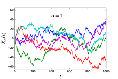
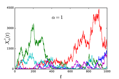
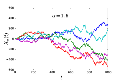
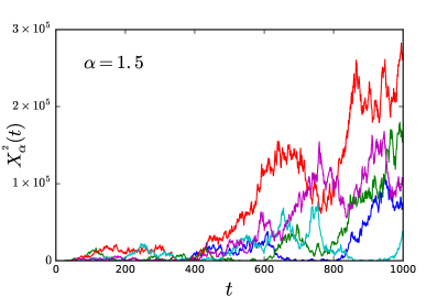
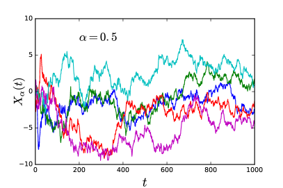
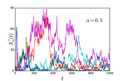
Figure 1: Four individual realisations $X_{\alpha}(t)$ for SBM with different anomalous diffusion exponent for subdiffusion ($\alpha=0.5$, top), normal diffusion ($\alpha=1$, middle), and superdiffusion ($\alpha=1.5$, bottom). In the left column we show the process $X_{\alpha}(t)$ itself, while in the right column we display its square, $X_{\alpha}^{2}(t)$.

2 Model and basic notations

SBM $X_{\alpha}(t)$ is an $\alpha$-parametrised family of Gaussian stochastic processes defined by the (stochastic) Langevin equation [22, 23, 24]

$$\frac{dX_{\alpha}(t)}{dt}=\sqrt{2D_{\alpha}(t)}\times\xi(t),$$ (3)

where $\xi(t)$ denotes Gaussian white-noise with zero mean and the variance $1/2$, such that

$$\langle\xi(t_{1})\xi(t_{2})\rangle=\delta(t_{1}-t_{2}),.$$ (4)

Moreover, $D_{\alpha}(t)$ is the diffusion coefficient, that follows the deterministic power-law in time

$$D_{\alpha}(t)=\alpha K_{\alpha}t^{\alpha-1},\quad 0<\alpha<2,$$ (5)

where the coefficient $K_{\alpha}$ has physical dimension $\mathrm{cm}^{2}/\mathrm{sec}^{\alpha}$. In general, SBM describes anomalous diffusion, such that the ensemble-averaged MSD scales as a power law in time,

$$\langle X_{\alpha}^{2}(t)\rangle=2K_{\alpha}t^{\alpha}.$$ (6)

When $0<\alpha<1$ one observes subdiffusive behaviour, while for $1<\alpha<2$ SBM describes superdiffusion. Standard Brownian motion is recovered in the limit $\alpha=1$. In figure 1 we depict four representative trajectories of $X_{\alpha}(t)$ for the subdiffusive, normal-diffusive, and superdiffusive cases. We note that, especially for the subdiffusive case $\alpha=1/2$ the non-stationary character is not immediately obvious from the graph of $X_{\alpha}(t)$, while the character of the process becomes somewhat more obvious when we plot the square process, $X_{\alpha}^{2}(t)$. Concurrently, in the superdiffusive case the growing fluctuations and large excursions away from the origin appear relatively more pronounced.

Before we proceed, it is expedient to recall other salient properties of SBM. In particular, its autocorrelation function can be readily calculated to give

$$\langle X_{\alpha}(t_{1})X_{\alpha}(t_{2})\rangle=2K_{\alpha}[\min\{t_{1},t_{2}\}]^{\alpha}.$$ (7)

Hence, the covariance of $X_{\alpha}(t)$ has essentially the same form as the one for standard Brownian motion, except that the time variable is "scaled". A basic quantity to analyse the behaviour of individual trajectories is the time-averaged MSD of the time series $X_{\alpha}(t)$ in the time interval $[0,T]$ [33],

$$\overline{\delta^{2}(\Delta)}=\frac{1}{T-\Delta}\int^{T-\Delta}_{0}\Big{(}X_{\alpha}(t+\Delta)-X_{\alpha}(t)\Big{)}^{2}dt,$$ (8)

and its ensemble-averaged counterpart, which, taking into account expression (7), can be explicitly calculated as [24]

$$\left<\overline{\delta^{2}(\Delta)}\right>=\frac{2K_{\alpha}}{\alpha+1}\left(\frac{T^{\alpha+1}-\Delta^{\alpha+1}}{T-\Delta}-(T-\Delta)^{\alpha}\right).$$ (9)

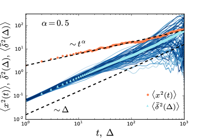
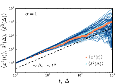
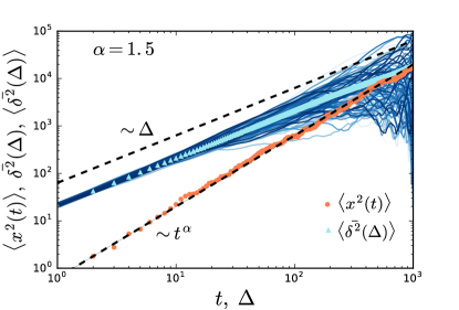
In the limit $\Delta\ll T$ we thus find $\langle\overline{\delta^{2}(\Delta)}\rangle\sim 2K_{\alpha}\Delta/T^{1-\alpha}$, a behaviour fundamentally different from the ensemble-averaged MSD (6), a feature of so-called weak ergodicity breaking: $\langle\overline{\delta^{2}(\Delta)}\rangle\neq\langle X_{\alpha}^{2}(\Delta)\rangle$ [33]. We display the behaviour of individual time-averaged MSDs $\overline{\delta^{2}(\Delta)}$ in figure 2, along with their ensemble average $\langle\overline{\delta^{2}(\Delta)}\rangle$ and the standard MSD $\langle X_{\alpha}^{2}(t)\rangle$. The non-ergodic behaviour of SBM is clearly highlighted by the different slopes of $\langle\overline{\delta^{2}(\Delta)}\rangle$ and $\langle X_{\alpha}^{2}(t)\rangle$.

Figure 2: SBM mean squared displacements (MSDs). For three different $\alpha$ values (subdiffusion with $\alpha=0.5$, top; normal diffusion with $\alpha=1$, middle; superdiffusion with $\alpha=1.5$, bottom). Blue lines represent time averaged MSDs $\overline{\delta^{2}(\Delta)}$ for individual trajectories. For small $\Delta\ll T$ the individual $\overline{\delta^{2}(\Delta)}$ are fully reproducible, while for longer lag time $\Delta$ the statistics becomes worse and the trajectory-to-trajectory spread is appreciable. The light blue line represents the trajectory-average $\langle\overline{\delta^{2}(\Delta)}\rangle$ of the time averaged MSD while the orange line depicts the ensemble averaged MSD $\langle x^{2}(t)\rangle$.

Equipped with all necessary knowledge on the properties of SBM $X_{\alpha}(t)$, we now turn to the question of interest here, the analysis of its single-trajectory PSD. As $S(f,T)$ is a random variable, the most general information about its properties is contained in the moment-generating function

$$\Phi_{\lambda}=\langle\exp\left(-\lambda S(f,T)\right)\rangle,\quad\lambda\geq 0.$$ (10)

Once $\Phi_{\lambda}$ is determined, the PDF $P(S(f,T)=S)$ of the random variable $S(f,T)$ can be simply derived from equation (10) by an inverse Laplace transform with respect to the parameter $\lambda$. As we proceed to show below, both $\Phi_{\lambda}$ and $P(S(f,T)=S)$ are entirely defined by the first two moments, due to the Gaussian nature of the process $X_{\alpha}(t)$. The mean value, which represents the standard time-dependent PSD, is given by

$$\mu(f,T)=\left\langle S(f,T)\right\rangle,$$ (11)

while the variance of the random variable $S(f,T)$ obeys

$$\sigma^{2}(f,T)=\left\langle S^{2}(f,T)\right\rangle-\mu^{2}(f,T).$$ (12)

The calculation of the exact explicit forms of the properties defined in equations (10) to (12) represents the chief goal of our work.

3 Spectral analysis of individual trajectories of scaled Brownian motion

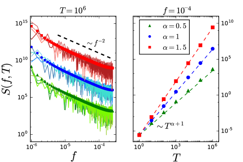
The single-trajectory PSDs $S(f,T)$ for four different sample trajectories for the three anomalous diffusion exponents $\alpha=1/2$, $\alpha=1$, and $\alpha=3/2$ are shown in figure 3. While, naturally, we observe distinct fluctuations within $S(f,T)$ and between different realisations, all data clearly show a $S(f,T)\simeq 1/f^{2}$-scaling. The right panel of figure 3 demonstrates the apparent scaling of the trajectory-averaged single-trajectory PSD as function of the observation time $T$ (ageing behaviour)—with the $T^{1+\alpha}$-scaling derived below. We are now going to quantify these behaviours in detail.

Figure 3: Left: Single trajectory power spectra $S(f,T)$ for subdiffusion ($\alpha=1/2$, top), normal diffusion ($\alpha=1$, middle), and superdiffusion ($\alpha=3/2$, bottom) as function of frequency $f$. The thick lines represent the mean of the simulated PSDs $S(f,T)$. The $1/f^{2}$ trend is indicated by the dashed line. Right: mean of $S(f,T)$, averaged over individual trajectories, as function of the observation time $T$.

3.1 Moment-generating function of the single-trajectory PSD

We start from definition (1) of the single-trajectory PSD and rewrite it in the form

$$S(f,T)=\frac{1}{T}\int_{0}^{T}\int_{0}^{T}\cos(f(t_{1}-t_{2}))X_{\alpha}(t_{1})X_{\alpha}(t_{2})dt_{1}dt_{2},$$ (13)

which is just a formal procedure since $X_{\alpha}(t)$ is a real-valued process. Relegating the intermediate steps of the derivation to A, we eventually find the exact result

$$\Phi_{\lambda} = \left\langle\exp\left(-\frac{\lambda}{T}\int_{0}^{T}\int_{0}^{T}\cos\left(f(t_{1}-t_{2})\right)X_{\alpha}(t_{1})X_{\alpha}(t_{2})dt_{1}dt_{2}\right)\right\rangle$$ (14)

$$= \frac{1}{\sqrt{1+2\mu\lambda+(2\mu^{2}-\sigma^{2})\lambda^{2}}},$$

where $\mu$ and $\sigma^{2}$ are defined in equations (11) and (12), respectively. Result (14) shows that the PDF of the single-trajectory PSD for SBM is fully defined through its first and second moment, and that it has exactly the same functional form as the results for Brownian motion and FBM derived in [16, 17]. As we have already remarked, this is a direct consequence of the Gaussian nature of the parental process $X_{\alpha}(t)$ of SBM.

Inverting the Laplace transform with respect to $\lambda$ we obtain the PDF of the random variable $S(f,T)$,

$$P(S(f,T)=S)=\frac{1}{\mu\sqrt{2-\gamma^{2}}}\exp\left(-\frac{S}{\mu(2-\gamma^{2})}\right)I_{0}\left(\frac{\sqrt{\gamma^{2}-1}}{\mu(2-\gamma^{2})}S\right),$$ (15)

where $\gamma=\sigma/\mu$ is the coefficient of variation of the PDF of the single-trajectory PSD for SBM, and $I_{\nu}$ is the modified Bessel function of the first kind. The latter is known to be a distribution with heavier-than-Gaussian tails.

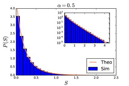
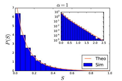
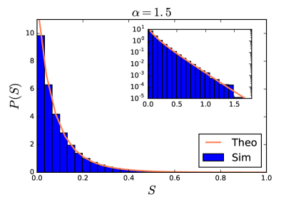
In figure 4 we present a comparison of the analytical result (15) for $P(S(f,T)=S)$ with simulations. The agreement is excellent. The width of the PDF $P(S(f,T)=S)$ becomes narrower for increasing $\alpha$ (note the different scales on the axes). In particular, the insets show the exponential shape of the PDF $P(S(f,T)=S)$ in the semi-logarithmic plots.

Figure 4: Amplitude PDF $P(S(f,T)=S)$ of single-trajectory PSDs for different values of the anomalous diffusion exponent: subdiffusive ($\alpha=1/2$, top), normal diffusive ($\alpha=1$, middle), and superdiffusive ($\alpha=3/2$, bottom). In the plots, "Theo" stands for the analytical result (15), while "Sim" is the histogram obtained from simulations, corresponding to averages over $10^{6}$ realisations for each $\alpha$. The insets report the same quantities on a semi-logarithmic scale, demonstrating that the large-$S$ tail of the PDF in equation (15) is an exponential function. Analytical and numerical results are in an excellent agreement.

3.2 Ensemble-averaged PSD

We now proceed further and calculate the first moment of the PSD, defined in equation (11). Recalling the expression for the autocorrelation function (7) of SBM, we perform the integrations explicitly in A, to find the final expression

$$\mu(f,T)=\frac{4K_{\alpha}T^{\alpha+1}}{fT}\left[\sin(fT)g_{1}\left(\frac{\alpha}{2},fT\right)-\cos(fT)g_{2}\left(\frac{\alpha}{2},fT\right)\right],$$ (16)

where we introduced the functions $g_{1}$ and $g_{2}$ defined in A. It is straightforward to check that for $\alpha=1$ equation (16) yields the standard expression of the PSD for Brownian motion,

$$\mu(f,T)\Big{|}_{\alpha=1}=\frac{4K_{1}}{f^{2}}\left(1-\frac{\sin(fT)}{fT}\right),$$ (17)

where $K_{1}$ is the normal diffusion coefficient of dimensionality $\mathrm{cm}^{2}/\mathrm{sec}$.

Next, we focus on the asymptotic behaviour of the general expression (11) in the limit $fT\to\infty$, which is equivalent to either the limit $f\to\infty$ with $T$ fixed, or vice versa. We get

$$\mu(f,T)\sim\frac{4K_{\alpha}T^{\alpha-1}}{f^{2}}\left\{1-\frac{\Gamma(\alpha+1)\cos(fT-\frac{\pi\alpha}{2})}{(fT)^{\alpha}}\right\}.$$ (18)

Interestingly, the $f$-dependence of the leading term is the same for any $\alpha$, in particular, it is equal to the one for Brownian motion. The fact that we are not able to distinguish SBM from Brownian motion by just looking at the frequency domain can lead, when analysing data, to the wrong conclusion that one deals with standard Brownian motion. Only when we have sufficiently precise data over a large frequency window, we could use the $\alpha$-dependent subleading term to identify the anomalous diffusion exponent $\alpha$. The only explicit $\alpha$-dependence in the leading order of expression (18) is in the ageing behaviour encoded by the dependence on $T^{\alpha-1}$ in the prefactor, which therefore becomes a relevant behaviour to check.

The dependence on $\alpha$ of the ageing factor leads to the convergence of the limit $T\to\infty$ in the subdiffusive case and to a divergence in the superdiffusive case. A second interesting limit is given by the low-frequency limit $f=0$. In this case we obtain

$$\mu(f=0,T)=\frac{4K_{\alpha}T^{\alpha+1}}{(\alpha+1)(\alpha+2)}.$$ (19)

This result represents the averaged squared area under the random curve $X_{\alpha}(t)$.

3.3 Variance and the coefficient of variation

The variance of the single-trajectory PSD is defined in equation (12). It can be calculated exactly for arbitrary $\alpha$, $f$ and $T$, and the details of the intermediate steps are presented in A. Here we report the asymptotic behaviour for $fT\to\infty$, reading

$$\sigma^{2}(f,T) \sim \frac{16K_{\alpha}^{2}T^{2\alpha-2}}{f^{4}}\left\{\frac{5}{4}+\frac{\Gamma^{2}(\alpha+1)}{(fT)^{2\alpha}}+\frac{2\Gamma(\alpha+1)\cos^{2}(fT-\frac{\pi\alpha}{2})}{2^{\alpha+2}(fT)^{\alpha}}\right.$$ (20)

$$-\frac{3\Gamma(\alpha+1)\cos(fT-\frac{\pi\alpha}{2})}{(fT)^{\alpha}}+\frac{\Gamma^{2}(\alpha+1)\cos^{2}(fT-\frac{\pi\alpha}{2})}{(fT)^{2\alpha}}$$

$$-\left.\frac{\Gamma^{2}(\alpha+1)}{2^{\alpha+2}(fT)^{2\alpha}}[4\cos(fT)-1]\right\}.$$

As for the mean value, the $f$-dependence of the leading term does not involve $\alpha$, and it has the same scaling as Brownian motion. Similarly, the explicit dependence on $\alpha$ of the frequence appears only in subleading order. Once again, studying the leading frequency scaling only we are not able to distinguish SBM from Brownian motion. Instead, we should pay attention to the ageing behaviour of the amplitude.

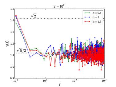
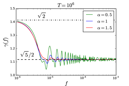
We summarise the results for the mean and variance of the single-trajectory PSD in the behaviour of the coefficient of variation, $\gamma$. It was shown that for FBM this dimensionless factor plays the role of a delicate key criterion to identifying anomalous diffusion. Namely $\gamma$ assumes three different values in the limit of large frequency depending on whether we have sub-, normal or superdiffusion, but independent of the precise value of $\alpha$. In the SBM case, recalling the asymptotic results for the mean and variance in equations (18) and (20) respectively, we obtain

$$\gamma\sim\sqrt{5}/2,\quad f\to\infty$$ (21)

for any $\alpha$. Moreover in the limit of $fT\to 0$ we obtain

$$\sigma^{2}(f=0,T)=\frac{32K^{2}_{\alpha}T^{2\alpha+2}}{(\alpha+1)^{2}(\alpha+2)^{2}}\quad\mbox{and}\quad\gamma\sim\sqrt{2}.$$ (22)

In this limit the moment-generating function simplifies and the probability density function is the gamma distribution with scale $2\mu(f=0,T)$ and shape parameter $1/2$.

In figure 5 analytical and numerical results for the coefficient of variation $\gamma$ are shown. Analytically, in the case of subdiffusion we observe heavier oscillation of $\gamma$ as function of the frequency, while in the superdiffusive case the convergence to the limiting value (21) is faster. Such a distinction is not so clear in the numerics, where the behaviour of $\gamma$ is essentially the same for the three different values of $\alpha$, showing again the difficulties in differentiating SBM from Brownian motion.

Figure 5: Left panel: analytical behaviour of $\gamma$ for 3 different values of $\alpha$ corresponding to sub-, normal and super-diffusion. Right panel: $\gamma$ obtained from $10^{3}$ realisations of SBM, each consisting of $N=10^{6}$ time steps.

3.4 Comparison with FBM

The results obtained for SBM show both similarities and dissimilarities with the ones for FBM reported in [17]. In fact, both processes share the same form for the PDF $P(x,t)$ in an infinite space and are therefore often confused with one another in literature, see the caveats raised in [24, 33]. However, while both processes are obviously Gaussian, FBM has stationary increments yet long-ranged, power-law noise correlations. In contrast, SBM is non-stationary but driven by uncorrelated noise. After our results above a natural question is whether in terms of the single-trajectory PSD the two processes can be told apart.

For the frequency dependence of the single-trajectory PSD $S(f,T)$, and thus also the mean $\mu(f,T)$, SBM shares the $1/f^{2}$ scaling with that of Brownian motion for any value of the anomalous diffusion exponent $\alpha$ in the range $0<\alpha<2$. Subdiffusive FBM, in contrast, exhibits a completely different behaviour with the explicitly $\alpha$-dependent frequency scaling $1/f^{\alpha+1}$. Moreover, while in the subdiffusive regime SBM shows the ageing dependence $\mu\simeq T^{\alpha-1}$, FBM is independent of $T$. Thus, SBM and FBM can be told apart quite easily from both $f$ and $T$ dependencies. In contrast, in the superdiffusive regime the results for SBM and FBM are the same for the functional behaviours with respect to both $f$ and $T$, and the processes therefore cannot be told apart from each other by use of the single-trajectory PSD or its mean. However, indeed there exists a difference when we consider the coefficient of variation $\gamma$. Namely, for SBM $\gamma$ always converges to the value $\gamma\sim\sqrt{5}/2$ at high frequencies, the value shared with Brownian motion. FBM, in contrast, assumes three distinct values in the high frequency limit: $\gamma\sim 1$ for subdiffusion ($0<\alpha<1$), $\gamma\sim\sqrt{5}/2$ for normal diffusion ($\alpha=1$), and $\gamma\sim\sqrt{2}$ for superdiffusion ($1<\alpha<2$). These predictions are confirmed by numerical and experimental data [16, 17]. The coefficient of variation therefore provides a suitable tool to distinguish SBM from FBM. We note that it is not necessary that the value of $\gamma$ has fully converged within the frequency window probed by experiment or simulation. It is sufficient to see from the data whether a clear trend for a departure from the value $\sqrt{5}/2$ assumed by Brownian motion and SBM.

4 Conclusions

We here studied the spectral content of SBM, a standard model for anomalous diffusion which is Markovian but non-stationary, in terms of the single-trajectory PSD and its full distribution. From analytical and numerical analyses we showed that the frequency dependence has the invariant scaling form $\sim 1/f^{2}$, fully independent of the anomalous scaling exponent $\alpha$. We also showed that the coefficient of variation for any $\alpha$ practically has the same frequency dependence as for Brownian motion. The main difference between SBM and Brownian motion is the ageing behaviour of single-trajectory PSD and its mean, that is, their dependence on the observation time $T$.

FBM, in contrast, has stationary increments yet is non-Markovian due to its power-law correlated driving noise. Both FBM and SBM are Gaussian in nature, and we found both emerging similarities and dissimilarities. For both sub- and superdiffusion the coefficient of variation for FBM provides different values from SBM. In addition, subdiffusive FBM is non-ageing but has an $\alpha$-dependent frequency scaling of the single-trajectory PSD. The situation is different in the superdiffusive regime: here the frequency dependence and the ageing behaviour of the single-trajectory PSD for FBM is the same as for SBM, leaving the coefficient of variation as the only way to distinguish the two processes from each other. Taking together all observables, we conclude that the single-trajectory PSD is able to distinguish SBM, FBM, and normal Brownian motion. We note that the PDF of the single-trajectory PSD is, however, the same for all three cases.

The results reported here for SBM adds an important additional piece to the development of a complete picture for single-trajectory PSD analysis of modern single particle tracking data. We demonstrated that it is a suitable tool to identify the anomalous scaling exponent $\alpha$ from an individual particle trajectory $X_{\alpha}(t)$. Moreover, within the Gaussian processes studied so far, the single-trajectory PSD framework allows one to tell the different processes apart from each other, and is thus an outstanding physical observable, providing complementary information to the (more) standard analyses in terms of ensemble and time averaged MSDs.

Appendix A Mean single-trajectory PSD

Recalling definition (18) we have

$$\mu(f,T) = \frac{1}{T}\int_{0}^{T}dt_{1}\int_{0}^{T}dt_{2}\cos(f(t_{1}-t_{2}))2K_{\alpha}\min(t_{1},t_{2})^{\alpha}$$ (23)

$$= \frac{2K_{\alpha}}{T}\int_{0}^{T}dt_{1}\left\{\int_{0}^{t_{1}}dt_{2}\cos(f(t_{1}-t_{2}))t_{2}^{\alpha}+\int_{t_{1}}^{T}dt_{2}\cos(f(t_{1}-t_{2}))t_{1}^{\alpha}\right\}$$

$$= \frac{2K_{\alpha}}{T}\left\{\int_{0}^{T}dt_{1}\int_{0}^{t_{1}}dt_{2}\left[\cos(ft_{1})\cos(ft_{2})+\sin(ft_{1})\sin(ft_{2})\right]t_{2}^{\alpha}\right.$$

$$\left.+\int_{0}^{T}dt_{1}\int_{t_{1}}^{T}dt_{2}\left[\cos(ft_{1})\cos(ft_{2})+\sin(ft_{1})\sin(ft_{2})\right]t_{1}^{\alpha}\right\}$$

$$= \frac{2K_{\alpha}}{T}\left\{I_{1}+I_{2}+I_{3}+I_{4}\right\}.$$

We focus on the explicit calculation of each integral individually, starting with

$$I_{1} = \int_{0}^{T}dt_{1}\int_{0}^{t_{1}}dt_{2}\cos(ft_{1})\cos(ft_{2})t_{2}^{\alpha}=\int_{0}^{T}dt_{1}\cos(ft_{1})\int_{0}^{t_{1}}dt_{2}\cos(ft_{2})t_{2}^{\alpha}$$ (24)

$$= T^{\alpha+2}\int_{0}^{1}dy\cos(\omega y)y^{\alpha+1}\int_{0}^{1}dz\cos(\omega yz)z^{\alpha}$$

$$= T^{\alpha+2}\int_{0}^{1}dy\cos(\omega y)y^{\alpha+1}g_{1}(\frac{\alpha}{2},\omega y),$$

where $\omega=fT$ and

$$g_{1}(\alpha,\omega) = \int_{0}^{1}\tau^{2\alpha}\cos(\omega\tau)d\tau$$ (25)

$$= -\frac{\Gamma(2\alpha+1)\sin(\pi\alpha)}{\omega^{2\alpha+1}}$$

$$-\frac{i}{2\omega^{2\alpha+1}}\left(\rme^{i\pi\alpha}\Gamma(2\alpha+1,-i\omega)-\rme^{-i\pi\alpha}\Gamma(2\alpha+1,i\omega)\right).$$

Similarly for the second integral we obtain

$$I_{2} = \int_{0}^{T}dt_{1}\sin(ft_{1})\int_{0}^{t_{1}}dt_{2}\sin(ft_{2})t_{2}^{\alpha}$$ (26)

$$= T^{\alpha+2}\int_{0}^{1}dy\sin(\omega y)y^{\alpha+1}g_{2}(\frac{\alpha}{2},\omega y),$$

where

$$g_{2}(\alpha,\omega) = \int_{0}^{1}\tau^{2\alpha}\sin(\omega\tau)d\tau$$ (27)

$$= \frac{\Gamma(2\alpha+1)\cos(\pi\alpha)}{\omega^{2\alpha+1}}$$

$$-\frac{1}{2\omega^{2\alpha+1}}\left(\rme^{i\pi\alpha}\Gamma(2\alpha+1,-i\omega)+\rme^{-i\pi\alpha}\Gamma(2\alpha+1,i\omega)\right).$$

Plugging in the explicit expressions of $g_{1}(\alpha,\omega)$ and $g_{2}(\alpha,\omega)$ and working out the integrals we arrive at

$$I_{1} = T^{\alpha+2}\left\{-\frac{\Gamma(\alpha+1)\sin(\pi\alpha/2)\sin(\omega)}{\omega^{\alpha+2}}-\frac{\Gamma(\alpha+1)\cos(\pi\alpha/2)}{(2\omega)^{\alpha+2}}\right.$$ (28)

$$-i\frac{\sin(\omega)}{2\omega^{\alpha+2}}\left[\rme^{i\pi\alpha/2}\Gamma(\alpha+1,-i\omega-\rme^{-i\pi\alpha/2}\Gamma(\alpha+1,i\omega)\right]$$

$$\left.+\frac{1}{2(2\omega)^{\alpha+2}}\left[\rme^{i\pi\alpha/2}\Gamma(\alpha+1,-2i\omega)+\rme^{-i\pi\alpha/2}\Gamma(\alpha+1,2i\omega)\right]\right\},$$

$$I_{2} = T^{\alpha+2}\left\{-\frac{\Gamma(\alpha+1)\cos(\pi\alpha/2)\cos(\omega)}{\omega^{\alpha+2}}+\frac{\Gamma(\alpha+1)\cos(\pi\alpha/2)}{(2\omega)^{\alpha+2}}\right.$$ (29)

$$+\frac{\cos(\omega)}{2\omega^{\alpha+2}}\left[\rme^{i\pi\alpha/2}\Gamma(\alpha+1,-i\omega)+\rme^{-i\pi\alpha/2}\Gamma(\alpha+1,i\omega)\right]$$

$$\left.-\frac{1}{2(2\omega)^{\alpha+2}}\left[\rme^{i\pi\alpha/2}\Gamma(\alpha+1,-2i\omega)+\rme^{-i\pi\alpha/2}\Gamma(\alpha+1,2i\omega)\right]\right\}.$$

The last two integrals are given by

$$I_{3} = \int_{0}^{T}dt_{1}\cos(ft_{1})t_{1}^{\alpha}\int_{t_{1}}^{T}dt_{2}\cos(ft_{2})$$ (30)

$$= \frac{T^{\alpha+2}}{\omega}\left\{\sin(\omega)g_{1}(\frac{\alpha}{2},\omega)-\frac{1}{2}\int_{0}^{1}dyy^{\alpha}\sin(2\omega y)\right\},$$

$$I_{4} = \int_{0}^{T}dt_{1}\sin(ft_{1})t_{1}^{\alpha}\int_{t_{1}}^{T}dt_{2}\sin(ft_{2})$$ (31)

$$= \frac{T^{\alpha+2}}{\omega}\left\{-\cos(\omega)g_{2}(\frac{\alpha}{2},\omega)+\frac{1}{2}\int_{0}^{1}dyy^{\alpha}\sin(2\omega y)\right\},$$

so that we finally obtain

$$\mu(f,T) = 2K_{\alpha}T^{\alpha+1}\left\{-\frac{\Gamma(\alpha+1)}{\omega^{\alpha+2}}\cos\left(\omega-\frac{\pi\alpha}{2}\right)\right.$$ (32)

$$+\frac{\cos(\omega-\frac{\pi\alpha}{2})}{2\omega^{\alpha+2}}\left[\Gamma(\alpha+1,i\omega)+\Gamma(\alpha+1,-i\omega)\right]$$

$$+\frac{i\sin(\omega-\frac{\pi\alpha}{2})}{2\omega^{\alpha+2}}\left[\Gamma(\alpha+1,i\omega)-\Gamma(\alpha+1,-i\omega)\right]$$

$$\left.+\frac{1}{\omega}\left[\sin(\omega)g_{1}(\frac{\alpha}{2},\omega)-\cos(\omega)g_{2}(\frac{\alpha}{2},\omega)\right]\right\},$$

which can be simplified to the form (16).

Appendix B Moment-generating function of the single-trajectory PSD

The moment-generating function is calculated as

$$\Phi_{\lambda} = \left\langle\exp\left\{-\lambda S(f,T)\right\}\right\rangle=\left\langle\exp\left\{-\frac{\lambda}{T}\int_{0}^{T}\int_{0}^{T}dt_{1}dt_{2}\cos(f(t_{1}-t_{2}))X_{\alpha}(t_{1})X_{\alpha}(t_{2})\right\}\right\rangle$$ (33)

$$= \left\langle\exp\left\{-\frac{\lambda}{T}\left[\int_{0}^{T}dt\cos(ft)X_{\alpha}(t)\right]^{2}-\frac{\lambda}{T}\left[\int_{0}^{T}dt\sin(ft)X_{\alpha}(t)\right]^{2}\right\}\right\rangle$$

$$= \frac{T}{4\pi\lambda}\int_{-\infty}^{+\infty}dz_{1}\int_{-\infty}^{+\infty}dz_{2}\exp\left(-T\frac{z_{1}^{2}+z_{2}^{2}}{4\lambda}\right)$$

$$\times\left\langle\exp\left\{iz_{1}\int_{0}^{T}dt\cos(ft)X_{\alpha}(t)+iz_{2}\int_{0}^{T}dt\sin(ft)X_{\alpha}(t)\right\}\right\rangle$$

$$= \frac{T}{4\pi\lambda}\int_{-\infty}^{+\infty}dz_{1}\int_{-\infty}^{+\infty}dz_{2}\exp\left(-T\frac{z_{1}^{2}+z_{2}^{2}}{4\lambda}\right)$$

$$\times\left\langle\exp\left\{i\int_{0}^{T}dt\xi(t)(z_{1}Q_{1}+z_{2}Q_{2})\right\}\right\rangle,$$

where we used the identity $\exp(-b^{2}/4a)=\sqrt{a/\pi}\int_{-\infty}^{+\infty}dx\exp(-ax^{2}+ibx)$ and we defined

$$Q_{1} = \sqrt{2D_{\alpha}(t)}\left(\frac{\sin(fT)}{f}-\frac{\sin(ft)}{f}\right),$$

$$Q_{2} = \sqrt{2D_{\alpha}(t)}\left(\frac{\cos(ft)}{f}-\frac{\cos(fT)}{f}\right).$$ (34)

We can now average over the exponential of Gaussian variable and obtain

$$\Phi_{\lambda} = \frac{T}{4\pi\lambda}\int_{-\infty}^{+\infty}dz_{1}\int_{-\infty}^{\infty}dz_{2}\exp\left(-T\frac{z_{1}^{2}+z_{2}^{2}}{4\lambda}\right)$$ (35)

$$\times\exp\left(-\frac{1}{2}\int_{0}^{T}dtz_{1}^{2}Q_{1}^{2}-\frac{1}{2}\int_{0}^{T}dtz_{2}^{2}Q_{2}^{2}-\int_{0}^{T}dtz_{1}z_{2}Q_{1}Q_{2}\right)$$

$$= \left[1+\frac{4\lambda}{T}\left(\frac{A+B}{2}\right)+\left(\frac{4\lambda}{T}\right)^{2}\frac{AB-C^{2}}{4}\right]^{-1/2},$$

where for the last equality we used the identity $\int_{-\infty}^{+\infty}dz_{1}\int_{-\infty}^{+\infty}dz_{2}\exp(-\alpha z_{1}^{2}+\beta z_{2}^{2}-2\gamma z_{1}z_{2})=\pi(\alpha\beta-\gamma^{2})^{-1/2}$ and we defined

$$A = \int_{0}^{T}dtQ_{1}^{2}=\frac{2K_{\alpha}T^{\alpha+2}}{\omega}\left[2\sin\omega g_{1}(\frac{\alpha}{2},\omega)-g_{2}(\frac{\alpha}{2},2\omega)\right],$$

$$B = \int_{0}^{T}dtQ_{2}^{2}=\frac{2K_{\alpha}T^{\alpha+2}}{\omega}\left[g_{2}(\frac{\alpha}{2},2\omega)-2\cos\omega g_{2}(\frac{\alpha}{2},\omega)\right],$$

$$C = \int_{0}^{T}dtQ_{1}Q_{2}=\frac{2K_{\alpha}T^{\alpha+2}}{\omega}\left[\sin\omega g_{2}(\frac{\alpha}{2},\omega)-\cos\omega g_{1}(\frac{\alpha}{2},\omega)+g_{1}(\frac{\alpha}{2},2\omega)\right].$$ (36)

It is possible to show that

$$\frac{(A+B)}{T} = \mu(f,T),$$ (37)

$$\frac{4(AB-C^{2})}{T^{2}} = 2\mu^{2}(f,T)-\sigma^{2}(f,T).$$ (38)

Relations (37) and (38) allows us to rewrite the moment-generating function as

$$\Phi_{\lambda}=\left[1+2\mu\lambda+(2\mu^{2}-\sigma^{2})\lambda^{2}\right]^{-1/2}.$$ (39)

Appendix C Variance of the single-trajectory PSD

In order to obtain the PSD variance, given in (12) we first focus on the calculation of the second moment,

$$\langle S^{2}(f,T)\rangle = \frac{1}{T^{2}}\left\langle\int_{0}^{T}\int_{0}^{T}dt_{1}dt_{2}\cos(f(t_{1}-t_{2}))X_{\alpha}(t_{1})X_{\alpha}(t_{2})\right.$$ (40)

$$\times\left.\int_{0}^{T}\int_{0}^{T}dt_{3}dt_{4}\cos(f(t_{3}-t_{4}))X_{\alpha}(t_{3})X_{\alpha}(t_{4})\right\rangle$$

$$= \frac{1}{T^{2}}\int_{0}^{T}\int_{0}^{T}\int_{0}^{T}\int_{0}^{T}dt_{1}dt_{2}dt_{3}dt_{4}\cos(f(t_{1}-t_{2}))\cos(f(t_{3}-t_{4}))$$

$$\times\langle X_{\alpha}(t_{1})X_{\alpha}(t_{2})X_{\alpha}(t_{3})X_{\alpha}(t_{4})\rangle.$$

Following the Wick/Isserlis theorem we have

$$\langle X_{\alpha}(t_{1})X_{\alpha}(t_{2})X_{\alpha}(t_{3})X_{\alpha}(t_{4})\rangle = \langle X_{\alpha}(t_{1})X_{\alpha}(t_{2})\rangle\langle X_{\alpha}(t_{3})X_{\alpha}(t_{4})\rangle$$ (41)

$$+\langle X_{\alpha}(t_{1})X_{\alpha}(t_{3})\rangle\langle X_{\alpha}(t_{2})X_{\alpha}(t_{4})\rangle$$

$$+\langle X_{\alpha}(t_{1})X_{\alpha}(t_{4})\rangle\langle X_{\alpha}(t_{3})X_{\alpha}(t_{2})\rangle.$$

This allows us to rewrite (40) as

$$\langle S^{2}(f,T)\rangle = \frac{1}{T^{2}}\left\{\left[\int_{0}^{T}\int_{0}^{T}dt_{1}dt_{2}\cos(f(t_{1}-t_{2}))\langle X_{\alpha}(t_{1})X_{\alpha}(t_{2})\rangle\right]^{2}\right.$$ (42)

$$+\int_{0}^{T}\int_{0}^{T}\int_{0}^{T}\int_{0}^{T}dt_{1}dt_{2}dt_{3}dt_{4}\cos(f(t_{1}-t_{2}))\cos(f(t_{3}-t_{4}))$$

$$\times\langle X_{\alpha}(t_{1})X_{\alpha}(t_{3})\rangle\langle X_{\alpha}(t_{2})X_{\alpha}(t_{4})\rangle$$

$$+ \int_{0}^{T}\int_{0}^{T}\int_{0}^{T}\int_{0}^{T}dt_{1}dt_{2}dt_{3}dt_{4}\cos(f(t_{1}-t_{2}))\cos(f(t_{3}-t_{4}))$$

$$\times\left.\langle X_{\alpha}(t_{1})X_{\alpha}(t_{4})\rangle\langle X_{\alpha}(t_{3})X_{\alpha}(t_{2})\rangle\right\}$$

$$= \mu^{2}(f,T)+\frac{4K_{\alpha}^{2}}{T^{2}}\left\{\int_{0}^{T}\int_{0}^{T}\int_{0}^{T}\int_{0}^{T}dt_{1}dt_{2}dt_{3}dt_{4}\cos(f(t_{1}-t_{2}))\cos(f(t_{3}-t_{4}))\right.$$

$$\times\min(t_{1},t_{3})^{\alpha}\min(t_{2},t_{4})^{\alpha}$$

$$+\int_{0}^{T}\int_{0}^{T}\int_{0}^{T}\int_{0}^{T}dt_{1}dt_{2}dt_{3}dt_{4}\cos(f(t_{1}-t_{2}))\cos(f(t_{3}-t_{4}))$$

$$\times\min(t_{1},t_{4})^{\alpha}\min(t_{2},t_{3})^{\alpha}\Big{\}}.$$

The variance is thus given by

$$\sigma^{2}(f,T) = \frac{8K_{\alpha}^{2}}{T^{2}}\int_{0}^{T}\int_{0}^{T}\int_{0}^{T}\int_{0}^{T}dt_{1}dt_{2}dt_{3}dt_{4}\cos(f(t_{1}-t_{2}))\cos(f(t_{3}-t_{4}))$$ (43)

$$\times\min(t_{1},t_{3})^{\alpha}\min(t_{2},t_{4})^{\alpha}$$

$$= \frac{8K_{\alpha}^{2}}{T^{2}}\left\{\int_{0}^{T}\int_{0}^{T}dt_{1}dt_{2}\cos(f(t_{1}-t_{2}))\int_{0}^{t_{1}}dt_{3}\int_{0}^{t_{2}}dt_{4}\cos(f(t_{3}-t_{4}))t_{3}^{\alpha}t_{4}^{\alpha}\right.$$

$$+2\int_{0}^{T}\int_{0}^{T}dt_{1}dt_{2}\cos(f(t_{1}-t_{2}))\int_{t_{1}}^{T}dt_{3}\int_{0}^{t_{2}}dt_{4}\cos(f(t_{3}-t_{4}))t_{1}^{\alpha}t_{4}^{\alpha}$$

$$+\left.\int_{0}^{T}\int_{0}^{T}dt_{1}dt_{2}\cos(f(t_{1}-t_{2}))\int_{t_{1}}^{T}dt_{3}\int_{t_{2}}^{T}dt_{4}\cos(f(t_{3}-t_{4}))t_{1}^{\alpha}t_{2}^{\alpha}\right\}$$

$$= \frac{8K_{\alpha}^{2}}{T^{2}}\left\{I_{5}+2I_{6}+I_{7}\right\}.$$

Following the same procedure used above for calculating the mean we can show that the integrals are given by

$$I_{5} = I_{1}^{2}+I_{2}^{2}+I_{8}^{2}+I_{9}^{2},$$ (44)

$$I_{6} = \frac{T^{\alpha+2}}{\omega}\left\{I_{1}\left[\sin(\omega)g_{1}\left(\frac{\alpha}{2},\omega\right)-\frac{g_{2}\left(\frac{\alpha}{2},2\omega\right)}{2}\right]\right.$$ (45)

$$+I_{8}\left[\frac{1}{2(\alpha+1)}+\frac{g_{1}(\frac{\alpha}{2},2\omega)}{2}-\cos(\omega)g_{1}\left(\frac{\alpha}{2},\omega\right)\right]$$

$$+I_{9}\left[-\frac{1}{2(\alpha+1)}+\frac{g_{1}(\frac{\alpha}{2},2\omega)}{2}+\sin(\omega)g_{2}\left(\frac{\alpha}{2},\omega\right)\right]$$

$$\left.+I_{2}\left[-\cos(\omega)g_{2}\left(\frac{\alpha}{2},\omega\right)+\frac{g_{2}(\frac{\alpha}{2},2\omega)}{2}\right]\right\},$$

$$I_{7} = \frac{T^{\alpha+2}}{\omega^{2}}\left\{\frac{1}{2(\alpha+1)^{2}}+g_{1}\left(\frac{\alpha}{2},\omega\right)^{2}+g_{2}\left(\frac{\alpha}{2},\omega\right)^{2}+\frac{g_{1}(\frac{\alpha}{2},2\omega)^{2}}{2}+\frac{g_{2}(\frac{\alpha}{2},2\omega)^{2}}{2}\right.$$ (46)

$$-\sin(\omega)\left[\frac{g_{2}(\frac{\alpha}{2},\omega)}{\alpha+1}+g_{1}\left(\frac{\alpha}{2},\omega\right)g_{2}\left(\frac{\alpha}{2},2\omega\right)-g_{2}\left(\frac{\alpha}{2},\omega\right)g_{1}\left(\frac{\alpha}{2},2\omega\right)\right]$$

$$-\left.\cos(\omega)\left[\frac{g_{1}(\frac{\alpha}{2},\omega)}{\alpha+1}+g_{1}\left(\frac{\alpha}{2},\omega\right)g_{1}\left(\frac{\alpha}{2},2\omega\right)+g_{2}\left(\frac{\alpha}{2},\omega\right)g_{2}\left(\frac{\alpha}{2},2\omega\right)\right]\right\},$$

where $I_{1}$ and $I_{2}$ are defined in (29) and

$$I_{8} = T^{\alpha+2}\left\{\frac{\Gamma(\alpha+1)\cos(\pi\alpha/2)\sin(\omega)}{\omega^{\alpha+2}}-\frac{\Gamma(\alpha+1)\sin(\pi\alpha/2)}{(2\omega)^{\alpha+2}}\right.$$ (47)

$$-\frac{\sin(\omega)}{2\omega^{\alpha+2}}\left[\rme^{i\pi\alpha/2}\Gamma(\alpha+1,-i\omega)+\rme^{-i\pi\alpha/2}\Gamma(\alpha+1,i\omega)\right]$$

$$\left.-\frac{1}{2\omega(\alpha+1)}-\frac{i}{2(2\omega)^{\alpha+2}}\left[\rme^{i\pi\alpha/2}\Gamma(\alpha+1,-2i\omega)-\rme^{-i\pi\alpha/2}\Gamma(\alpha+1,2i\omega)\right]\right\},$$

$$I_{9} = T^{\alpha+2}\left\{-\frac{\Gamma(\alpha+1)\sin(\pi\alpha/2)\cos(\omega)}{\omega^{\alpha+2}}-\frac{\Gamma(\alpha+1)\sin(\pi\alpha/2)}{(2\omega)^{\alpha+2}}\right.$$ (49)

$$+i\frac{\cos(\omega)}{2\omega^{\alpha+2}}\left[\rme^{i\pi\alpha/2}\Gamma(\alpha+1,-i\omega-\rme^{-i\pi\alpha/2}\Gamma(\alpha+1,i\omega)\right]$$

$$+\left.\frac{1}{2\omega(\alpha+1)}-\frac{i}{2(2\omega)^{\alpha+2}}\left[\rme^{i\pi\alpha/2}\Gamma(\alpha+1,-2i\omega)-\rme^{-i\pi\alpha/2}\Gamma(\alpha+1,2i\omega)\right]\right\}.$$

References

• [1] M. P. Norton and D. G. Karczub, Fundamentals of Noise and Vibration Analysis for Engineers (Cambridge University Press, Cambridge UK, 2003).
• [2] Voss R and Clarke J 1975 Nature (London) 258 317.
Hennig H, Fleischmann R, Fredebohm A, Hagmayer Y, Nagler J, Witt A, Theis F J and Geisel T 2011 PLoS ONE 6 e26457.
• [3] Weber R O and Talkner P 2001 J. Geophys. Res. 106 20131.
• [4] Sornette A and Sornette D 1989 Europhys. Lett. 9 197.
• [5] Kirchner J W, Feng X and Neal C 2000 Nature (London) 403 524.
See also H. Scher, G. Margolin, R. Metzler, J. Klafter, and B. Berkowitz, Geophys. Res. Lett. 29, 1061 (2002).
• [6] Balandin A A 2013 Nat. Nanotechnol. 8 549.
• [7] Frantsuzov P A, Volkán-Kacsó S and Jank B 2013 Nano Lett. 13 402.
• [8] Krapf D 2013 Phys. Chem. Chem. Phys. 15 459.
• [9] Zorkot M, Golestanian R and Bonthuis D J 2016 Nano Lett. 16 2205.
• [10] Niemann M, Kantz H and Barkai E 2013 Phys. Rev. Lett. 110 140603.
Sadegh S, Barkai E and Krapf D 2014 New J. Phys. 16 113054.
• [11] Leibovich N, Dechant A, Lutz E and Barkai E 2016 Phys. Rev. E 94 052130.
• [12] Leibovich N and Barkai E 2017 Eur. Phys. J. B 90 229.
• [13] Majumdar S N and Oshanin G 2018 J. Phys. A 51 435001.
• [14] Bénichou O, Krapivsky P L, Mejía-Monasterio C and Oshanin G 2016 Phys. Rev. Lett. 117 080601.
• [15] Marinari E, Parisi G, Ruelle D and Windey P 1983 Phys. Rev. Lett. 50 1223.
Dean D S, Iorio A, Marinari E and Oshanin G 2016 Phys. Rev. E 94, 032131.
• [16] Krapf D, Marinari E, Metzler R, Oshanin G, Xu X & Squarcini A 2018 New J. Phys. 20 023029.
• [17] Krapf D, Lukat N, Marinari E, Metzler R, Oshanin G, Selhuber-Unkel C, Squarcini A, Stadler L, Weiss M & Xu X 2019 Phys. Rev. X 9 011019.
• [18] Schnellbächer N D and Schwarz U S 2018 New J. Phys. 20 031001.
• [19] Nørregaard K, Metzler R, Ritter C M, Berg-Sørensen K and Oddershede L B 2017 Chem. Rev. 117 4342.
Höfling F & Franosch T 2013 Rep. Progr. Phys. 76, 046602.
• [20] Kemp D B, Eichenseer K and Kiessling W 2015 Nat. Commun. 6 8890.
• [21] Tóth B, Lempérière Y, Deremble C, de Lataillade J, Kockelkoren J and Bouchaud J-P 2011 Phys. Rev. X 1 021006.
A. G. Cherstvy, D. Vinod, E. Aghion, A. V. Chechkin, and R. Metzler, New J. Phys. 19, 063045 (2017).
• [22] Lim S C & Muniandy S V 2002 Phys. Rev. E 66 021114.
Fulinski A 2011 Phys. Rev. E 83 061140.
Fulinski A 2013 J. Chem. Phys. 138 021101.
Fulinski A 2013 Acta Phys. Pol. 44 1137.
• [23] Thiel F & Sokolov I 2014 Phys. Rev. E 89 012115.
Safdari H, Cherstvy A G, Chechkin A V, Thiel F, Sokolov I M & Metzler R 2015 J Phys. A: Math. Theor. 48 375002.
• [24] Jeon J-H, Chechkin A V & Metzler R 2014 Phys. Chem. Chem. Phys. 16 15811.
• [25] Richardson L F 1926 Proc. R. Soc. A 110 709.
• [26] Batchelor G K 1952 Math. Proc. Camb. Phil. Soc. 48 345.
• [27] Bodrova A, Chechkin A V, Cherstvy A G & Metzler R 2015 Phys. Chem. Chem. Phys. 17 21791.
• [28] Oshanin G & Moreau M 1995 J. Chem. Phys. 102 2977.
• [29] Saxton M J 2001 Biophys. J. 75 2226.
Periasamy N & Verkman A S 1998 Biophys. J. 75 557.
• [30] Wu J & Berland M 2008 Biophys. J 95 2049.
• [31] Molini A, Talkner P, Katul G G & Porporato A 2011 Physica A 390 1841.
• [32] Bodrova AS, Chechkin AV, Cherstvy AG & Metzler R 2015 New J. Phys. 17, 063038.
• [33] R. Metzler, J.-H. Jeon, A. G. Cherstvy, and E. Barkai, Phys. Chem. Chem. Phys. 16, 24128 (2014).
E. Barkai, Y. Garini, and R. Metzler, Phys. Today 65(8), 29 (2012).
• [34] J.-P. Bouchaud, J. Phys. (Paris) I 2, 1705 (1992).
G. Bel and E. Barkai, Phys. Rev. Lett. 94, 240602 (2005).
A. Rebenshtok and E. Barkai, Phys. Rev. Lett. 99, 210601 (2007).
M. A. Lomholt, I. M. Zaid, and R. Metzler, Phys. Rev. Lett. 98, 200603 (2007).
G. Aquino, P. Grigolini, and B. J. West, Europhys. Lett. 80, 10002 (2007).