GEE: A Gradient-based Explainable Variational Autoencoder for Network Anomaly Detection
Abstract
This paper looks into the problem of detecting network anomalies by analyzing NetFlow records. While many previous works have used statistical models and machine learning techniques in a supervised way, such solutions have the limitations that they require large amount of labeled data for training and are unlikely to detect zero-day attacks. Existing anomaly detection solutions also do not provide an easy way to explain or identify attacks in the anomalous traffic. To address these limitations, we develop and present GEE, a framework for detecting and explaining anomalies in network traffic. GEE comprises of two components: (i) Variational Autoencoder (VAE) — an unsupervised deep-learning technique for detecting anomalies, and (ii) a gradient-based fingerprinting technique for explaining anomalies. Evaluation of GEE on the recent UGR dataset demonstrates that our approach is effective in detecting different anomalies as well as identifying fingerprints that are good representations of these various attacks.
Index Terms:
Anomaly Detection, NetFlow Records, Gradient-based FingerprintingI Introduction
Anomalies in network can arise due to attacks and threats in the cyberspace, such as different kinds of DDoS attacks (e.g., TCP SYN flooding, DNS amplification attacks, etc.), brute force attempts, botnet communications, spam campaign, network/port scans, etc. Network anomalies may also manifest due to non-malicious causes, such as faults in network, misconfigurations, BGP policy updates, changes in user behaviors, etc. Detection of anomalies, possibly in real time, is of utmost importance in the context of network security, in particular as we are currently witnessing a continuous change in the threat landscape, leading to increase in the intensity, sophistication and types of attacks [1]. This trend is expected to continue as the IoT market keeps expanding. Indeed, cyber criminals now target to harness more resources by exploiting IoT devices that are, both, likely to be much more vulnerable than typical computers and huge in number (e.g., Mirai attack [2]).
In this paper, we look into the problem of detecting anomalies in large-scale networks, like that of an Internet Service Provider (ISP). While the problem of network anomaly detection has been of keen interest to the research community for many years now, it still remains a challenge for a number of reasons. First, the characteristics of network data depend on a number of factors, such as end-user behavior, customer businesses (e.g., banking, retail), applications, location, time of the day, and are expected to evolve with time. Such diversity and dynamism limits the utility of rule-based detection systems.
Next, as capturing, storing and processing raw traffic from such high capacity networks is not practical, Internet routers today have the capability to extract and export meta data such as NetFlow records [3]. With NetFlow, the amount of information captured is brought down by orders of magnitude (in comparison to raw packet capture), not only because a NetFlow record represents meta data of a set of related packets, but also because NetFlow records are often generated from sampled packets. Yet, NetFlow records collected from a modest edge router with 24x10Gbps links for a 5-minute interval can easily reach a few GBs. However, with NetFlow, useful information such as suspicious keywords in payloads, TCP state transitions, TLS connection handshake, etc. are lost; indeed with sampled NetFlow, even sizes of each packet, time between consecutive packets, etc. are unavailable. Therefore, anomaly detection solutions have to deal with lossy information.
Finally, the SOC (security operation center) analysts have a limited budget, within which they have to analyze the alerts raised by an anomaly detector, for purposes such as alert escalation, threat and attack mitigation, intelligence gathering, forensic analysis, etc. Therefore, anomaly detectors should go beyond merely indicating the presence of anomalies; the time of anomaly, its type, and the corresponding set of suspicious flows are in particular very useful for further analysis. In general, the more the information that can be passed (along with the alerts) to the analysts, the easier is the task of analysis and quicker the decision process.
One way to address the above challenges is to apply statistical models and machine learning algorithms. Considering anomaly detection as a binary classification problem, a supervised machine learning model can be built using normal and anomalous data, for classifying anomalies. However, existing approaches have the following limitations. First, many of them exploit only a small number of features (e.g. traffic volume, flow rates, or entropy) [4, 5, 6]. Such approaches require the users to apply domain knowledge to select the right set of features which may not always be feasible and optimal. Second, supervised approaches require large sets of data with ground truth for training. Note that as the network characteristics and attacks evolve, models have to be retrained and the corresponding labeled datasets have to be made available. This requires costly and laborious manual efforts, and yet, given the size of traffic flowing through backbone network, it is highly impractical to assume all data records to be correctly labeled [7]. Besides, supervised approaches are unlikely to detect unknown and zero-day attack traffic.
To address these limitations, in this paper, we develop and present GEE, a gradient-based explainable variational autoencoder, for detecting as well as explaining anomalies in large-scale networks. GEE comprises of two important components: (i) a variational autoencoder (VAE), an unsupervised, deep-learning technique for detecting anomalies in network traffic; and (ii) a gradient-based fingerprinting technique for explaining threats and attacks in anomalous traffic. GEE addresses the limitations of existing approaches in the following way. First, modeling with VAE allows the use of a large number of features from the dataset thus relieving the need to employ domain knowledge to select the “right” set of features. Second, GEE works with unlabeled NetFlow traces which is the norm in ISP networks for data collection. Finally, GEE provides explanation as to why an anomaly is detected.
To summarize, the contributions of this paper are as follow:
-
•
We present a VAE based framework for network anomaly detection that is scalable in, both, the size of data and the feature dimension.
-
•
We develop a gradient-based framework to explain the detected anomalies, and identify the main features that cause the anomalies. This is of great impact in practice as deep learning techniques are notorious for non-interpretability.
-
•
Our framework GEE makes it possible to identify network attacks using gradient-based fingerprints generated by the VAE algorithm. To the best of our knowledge, this is the first attempt to explain network anomalies using gradients generated from a VAE model.
Evaluation using the UGR dataset [8] shows that GEE is effective in identifying the network attacks present, such as Spam, Botnet, (low-rate) DoS and port scans. Using GEE, we can identify the features that define these attacks and the fingerprints derived (when ground truth is available) can be utilized to further improve the detection accuracy.
II Related Work
Detection of network anomalies (such as threats, intrusions, attacks, etc.) is a widely and deeply studied research problem. Past works have developed solutions based on varying approches, for example, rule-based systems [9], information theoretic techniques [10, 11], signal analysis [12], statistical models and hypothesis testing [13, 14], as well as data mining and machine learning algorithms [15, 16]. As computational resources becoming cheaper, there has been an increasing interest in applying machine learning techniques for detecting anomalies in network. In the following, we present an overview of machine learning techniques applied on NetFlow data (or other forms of aggregate data usually collected from routers in ISP networks), for the purpose of detecting anomalies.
PCA (Principal Component Analysis) has been used to separate traffic space into two different subspaces (‘normal’ and ‘anomalous’) for anomaly detection. Aggregate byte counts of links in an ISP network was initially used as a feature [17]; and in Lakhina et al. [4], the solution was extended to work on more granular data. An inherent disadvantage of PCA is that the components in the reduced subspace do not provide an interpretation of features in the original space. Besides, as later studies have shown [18, 19], there are other challenges, an important one being that PCA-based detection solution is highly sensitive to the dimension of normal subspace and the detection threshold, both of which are not easily determined.
Another approach to detect anomalies is to first model the normal traffic, and then use a statistical decision theoretic framework to detect deviation from normal data. For example, Simmross-Wattenberg et al. [13] used -stable distributions to model 30-minute time bins of aggregate traffic rate, and generalized likelihood ratio test for classifying whether the time windows are anomalous. Since a number of parameters have to be learned, large amounts of labeled data have to be continuously made available for the model to adapt with time.
In Bilge et al. [16], a Random Forests classifier was trained to detect C&C servers in a supervised way, using features extracted from labeled NetFlow records. To reduce false positive rate, however, the system relies on reputation systems such as malicious domain classification system, Google Safe Browsing, etc. This affects detection accuracy since most recent botnets and evasive botnets may not have a low reputation score.
More recently, deep neural network models (also generally referred to as deep learning models) have been embraced by the research community to tackle anomaly detection problem in networking setting. Existing supervised deep learning approaches include work by Tang et al. [20] that utilizes a classical deep neural network for flow-based anomalies classification in a Software Defined Networking (SDN) environment, and use of the recurrent neural network (RNN) models for developing intrusion detection solution [21].
There are recent works that use unsupervised deep learning models to transform the data into lower rank features before applying supervised machine learning. Several prior approaches first employ autoencoders [22] and their variants to extract the compressed latent representation as features, and subsequently use these features for anomaly detection by training standard classifiers such as Random Forests [23].
Anomaly detection methods that are solely based on unsupervised deep learning models have also been experimented. These models do not require labeled information and instead exploit the fact that anomalous behaviors tend to differ greatly from the standard or normal behavior of the network. Fiore et al. [24] made use of discriminative restricted Boltzmann machine (RBM) for anomaly detection on network data; while Mirsky et al. [25] proposed an ensembles of light-weight autoencoders for real time network intrusion detection, although their focus is on scalability of the system. Further, An and Cho [26] demonstrated that the VAE performs much better than AE and PCA on handwritten digit recognition and network intrusion detection. However, the VAE model was trained using data labeled as normal, i.e., the anomalies are removed from training, which is difficult to do in practice. The above [24, 25, 26] are also known as semi-supervised learning.
Different from the above, we develop an anomaly detector using an unsupervised deep learning technique without using labeled information. While existing works (e.g., [26]) stop at the task of anomaly detection, in our work, we also provide a gradient-based technique for explaining why the anomalies are detected, together with their relevant features.
III Unsupervised Deep Learning Models
Given large amount of data being constantly collected by the network routers, existing anomaly detection frameworks tend to employ simple methods such as threshold-based approaches or simply PCA for scalability reason. Within the past decade, however, we see a rise of application of deep learning models due to their ability to handle big datasets as well as to train real-time in a streaming manner. This is while retaining their state-of-the-art performance in various tasks like real time object recognition [27] and fraud detection [28].
Additionally, deep learning models like the variational autoencoder (VAE) are shown to be robust to noisy data [29], and thus especially suitable for modeling network flows which are very noisy in nature. Although deep learning models are often criticized for their lack of interpretability, recent advances have brought forward better understanding of these models, in particular, attributing the causes to the results [30].
We focus on the VAE, a probabilistic generalization of the AE, for anomaly detection on network data. Note that the VAE has been shown to be more flexible and robust [26] compared to the AE. Further, we demonstrate how we can use gradient information from the VAE for interpretation purpose. For instance, it can be used to analyze how a certain set of features is more likely to explain a certain anomaly. In the following, we first describe the AE model since the VAE has the same deep architecture as the AE.
III-A Autoencoder (AE)
An AE is made of three main layers which correspond to (i) the input layer to take in the features, (ii) the latent representation layer of the features, and (iii) the output layer which is the reconstruction of the features. The AE consists of two parts called encoder and decoder respectively. The encoder maps the input into its latent representation while the decoder attempts to reconstruct the features back from the latent representation. The encoder may be deep in the sense that information from the input is passed through several mappings (and hidden layers) similar to the deep architecture in a supervised deep learning model; likewise for the decoder. In this paper, we set the size of the latent representation layer to be 100. In addition, the encoder and the decoder each have three hidden layers with size 512, 512, and 1,024 respectively, as illustrated in Fig. 1. In the figure, nodes that are shaded represent the observed data (used as both inputs and outputs), while the unshaded nodes are unobserved latent variables corresponding to the hidden layers. The exact size or dimension of the layers is shown above the nodes.
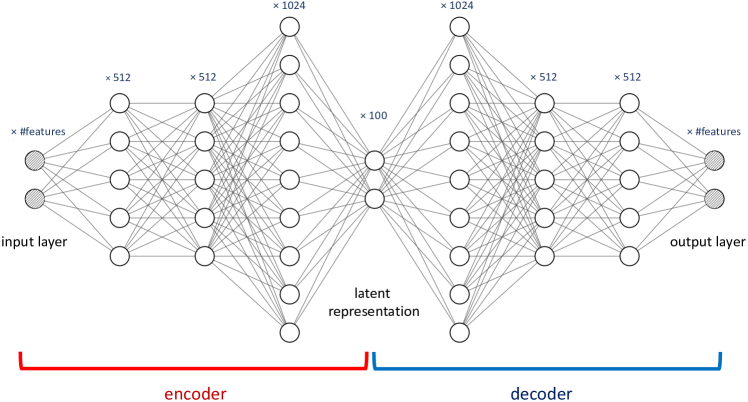
The links between the layers show how the values of the next layer can be computed. Commonly, the value of one hidden layer can be computed as
| (1) |
where is a vector of values for the previous layer, is a matrix of weights that signifies the relationship from the previous layer, and is a vector of bias terms. Both and are parameters to be learned through model training. Here, is known as the activation function that transforms the computation in a non-linear way and allows complex relationship to be learned. Popularly used activation functions include the sigmoid function and the rectified linear unit (ReLU) , which will be used in this paper. The learning of the parameters are generally achieved by minimizing the reconstruction errors (e.g., mean square errors) via backpropagation with random initialization, and can be optimized with a variety of optimizers such as stochastic gradient descent. We refer the readers to Bengio [31] and references therein for details on optimization.
In essence, we can view the AE as a deterministic model that maps a set of inputs (features in our case) into their reconstruction. This is in contrast to the generative model variants of deep neural network, such as the VAE and generative adversarial network (GAN), which is capable of generating new data based on the distribution of the training data.
III-B Variational Autoencoder (VAE)
Unlike AE that deterministically encodes the inputs into their latent representation and subsequently produce a reconstruction, the VAE [32] is a generative model that treats the latent representation layer as random variables conditional on the inputs. Although the encoder and decoder in the VAE follows the same computation model as the AE as in Equation (1), the encoding process is instead used to compute the parameters for the conditional distributions of the latent representation. The parameters can then be used to generate or sample the latent representation for decoding. The conditional distributions are generally assumed to be Gaussian for real-valued nodes. For example, denote as the value of the latent representation layer, then it can be written as
| (2) |
where denotes a function that transforms a vector into a diagonal matrix; and and are the mean and variance for the conditional Gaussian distribution obtained from the output of the encoder:
| (3) | ||||
| (4) |
The parameters , , , and are interpreted in the same way as in the autoencoder above. Treatment on the hidden layers is identical to that of autoencoder.
The probabilistic nature of the VAE also means that we cannot simply employ the usual learning algorithm on standard objective function (e.g. mean square error) to train the model. Instead, a class of approximate statistical inference method are used, which is called the Variational Bayes (thus gives rise to the name VAE). As the discussion on the inference methods are rather technically involved, we refer the interested readers to Kingma and Welling [32] for details. Put simply, an alternative objective function known as the variational lower bound is optimized, and stochastic sampling is used for approximation.
In terms of architecture, VAE is similar to AE and is illustrated in Fig. 1. The ReLU activation function is used by the encoder and the decoder in all of the intermediate layers, and the linear activation will be used for the output.
IV GEE: Anomaly Detection Framework
Our anomaly detection framework GEE consists of the following main steps. First, important information from the NetFlow data, such as the average packet size, entropy of destination ports, etc., are extracted to obtain a set of features. Then, the features are fed into the VAE for learning the normal behaviour of the network. Subsequently, anomalies are identified based on their reconstruction errors. Finally, we describe how we can employ the gradient information available from the VAE for explanation and for fingerprinting attacks.
IV-A Feature Extraction
A NetFlow record is a set of packets that has the same five-tuple of source and destination IP addresses, source and destination ports, and protocol. In addition to the above, some of the important fields that are commonly available in NetFlow records are start time of the flow (based on the first sampled packet), duration, number of packets, number of bytes, and TCP flag. We group the NetFlow records into 3-minute sliding windows based on the source IP addresses to form aggregated features. This means that each data point in this paper corresponds to the network statistics of a single source IP address within a 3-minute period. Note that such extraction allows us to identify the offending IP address and also the time window an anomaly belongs to, which are important for further analysis and decision making. The period of 3 minutes is chosen to balance between the practicality and quality of the aggregated statistics, where the statistics will be insignificant if the period is too short; while using a long time window means we cannot perform real time analysis.
Overall, we extract 53 aggregated features, which include
-
•
mean and standard deviation of flow durations, number of packets, number of bytes, packet rate; and byte rate;
-
•
entropy of protocol type, destination IP addresses, source ports, destination ports, and TCP flags; and
-
•
proportion of ports used for common applications (e.g. WinRPC, Telnet, DNS, SSH, HTTP, FTP, and POP3).
To ensure that meaningful statistics are captured, data point that contains too few flows (less than 10 in this case) are removed from the dataset. This reduces noise in the training data. Finally, the statistics are either scaled to between 0 and 1 or normalized into Z-score [33] as input features for the VAE.
IV-B Unsupervised Learning of VAE
Training algorithm of the VAE is implemented using TensorFlow [34], which provides powerful tools of automatic differentiation and comes with built-in optimization routines. As pointed out in Section III, the training of the VAE is fairly complex and beyond the scope of this paper, so we provide only a brief outline here. Before starting the training procedure, the parameters in the VAE are randomly initialized. This subsequently allows us to perform a forward pass on the encoder by computing the distribution of the latent representation layer via Equation (2). With this, several samples can be generated from the Gaussian distribution which are used to compute the variational lower bound, which consists of a KL divergence term and an expectation term:
| (5) |
where is the latent representation of the input features . Here, the distribution corresponds to the Gaussian prior and conditional distribution of the VAE model; while is a variational approximation [35] of , generally chosen to be Gaussian as well. Refer to Kingma and Welling [32] for details. Fortunately, this objective function can be maximized with stochastic optimization techniques since the gradients are readily available via automatic differentiation [36].
Here, we employ Adam [37] as the optimization algorithm, which enables training in minibatches. Generally, real-time training can be achieved by choosing a small minibatch size and discarding the data after one epoch. We like to highlight that label information is not used at all during training.
IV-C Anomaly Detection
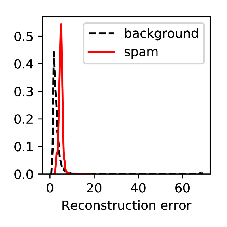
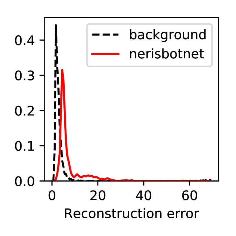
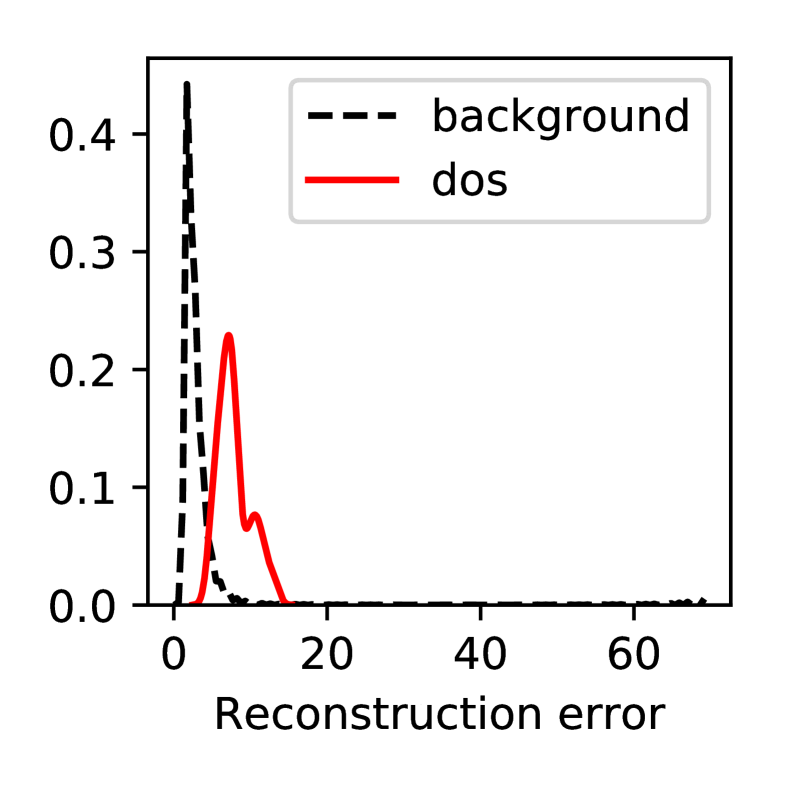
Once the parameters are optimized after training, the VAE model is used for anomaly detection, where an IP address and its time window is recognized as abnormal when the reconstruction error of its input features is high. Here, the reconstruction error is the mean square difference between the observed features and the expectation of their reconstruction as given by the VAE. A high reconstruction error is generally observed when the network behavior differs greatly from the normal behavior that was learned by the VAE. The threshold is usually selected such that we treat a small percentage (say 5%) of the data as anomalies. Otherwise, we can make use of the labeled information to select a threshold to maximize the detection rate while having small false positive rate. An illustration of how this can be done is suggested in the next section, with the aid of Fig. 2. Note the anomalies are associated with unusual network behaviours from a particular source IP address, and may not necessarily be malicious.
IV-D Gradient-based Explanation for Anomalies
While most existing anomaly detection works in the literature consider only the evaluation on detection accuracy, we go beyond and provide an explanation on why a data point is flagged as abnormal. This is significant since it challenges the popular belief that a deep learning model functions as a black box that cannot be interpreted; a VAE model can in fact be used to explain why an IP address is treated as an anomaly. This is done by analyzing the gradients ‘contributed’ by each feature of the data point, which is obtainable from the VAE through automatic differentiation in TensorFlow.
The key question to ask that leads to our approach is: How does the VAE’s objective function vary if a feature in the anomaly data point increases or decreases by a small amount? Intuitively, given the trained VAE and an anomalous data point, if the function (reconstruction error) changes quite a lot when a particular feature of the anomalous data point is varied by a small amount, then this feature at its current value is significantly abnormal, since it would like to perturb the VAE model (through optimization) to fit itself better.
Gradients, or more technically the derivative of the variational lower bound, , are computed for each feature from each data point . Two applications of the gradient can be immediately derived. Firstly, even without having the ground truth labels, the flagged anomalies can be clustered based on their gradients into groups that share similar behavior, making it easier for analysts to investigate. Secondly, if we have the labeled information on certain types of attacks, then we can derive gradient-based fingerprints that associate with the attacks. These fingerprints can be used to identify specific attacks from another day. Of course, the anomalies that are identified through the fingerprints are more accurate since labeled information was indirectly used in a way similar to semi-supervised learning. The anomalies are detected through the L2 distance computed from the normalized gradient vectors. The rationale of using such formulae is presented next.
V Dataset and Evaluation
| Date (2016) | Total | DoS | B.net | Sc11 | Sc44 | Spam | B.list |
| Training Set | |||||||
| Mar 19 (Sat) | 110M | - | - | - | - | ||
| Jul 30 (Sat) | 110M | - | |||||
| \hdashlineTest Set | |||||||
| Mar 18 (Fri) | 40M | - | - | - | - | ||
| Mar 20 (Sun) | 110M | - | - | - | - | ||
| July 31 (Sun) | 105M | - |
For evaluation, we use the recently published UGR16 dataset [8], which contains anonymized NetFlow traces captured from a real network of a Tier 3 ISP. The ISP provides cloud services and is used by many client companies of different sizes and markets. The UGR trace is a fairly recent and large-scale data trace that contains real background traffic from a wide range of Internet users, rather than specific traffic patterns from synthetically generated data (e.g., DARPA’98 and DARPA’99 [38], UNB ISCX 2012 [39], UNSW-NB15 [40], CTU13 [41]). Another publicly available Internet traffic data is from the MAWI Working Group [42], but the labeled data consists of only 15-minute of traffic per day. On the other hand, UGR contains traffic for the whole day over a 4-month period. Furthermore, UGR attack traffic data is a mixture of generated attacks, labeled real attacks, and botnet attacks from controlled environment. Specifically, the labeled attacks consist of:
-
•
Low-rate DoS: TCP SYN packets are sent to victims with packet of size 1280 bits and of rate 100 packets/s to port 80. The rate of the attack is sufficiently low such that the normal operation of the network is not affected.
-
•
Port scanning: a continuous SYN scanning to common ports of victims. There are two kinds of scanning, one-to-one scan attack (Scan11) and four-to-four (Scan44).
-
•
Botnet: a simulated botnet traffic obtained from the execution of the Neris malware. This data comes from the CTU13 trace [41].
-
•
Spam: peaks of SMTP traffic forming a spam campaign.
-
•
Blacklist: flows with IP addresses published in the public blacklists. As emphasized in UGR [8], not all traffic flows involving blacklisted IP addresses are related to attacks. However, we include it for completeness.
Other attack labels that are available in the dataset are ignored due to their low number of occurrence, as they appear in less than 10 flows in total. Also, we like to caution that the background traffic should not be treated as fully free of attacks, since it is likely that some attacks have avoided detection.
We select a total of five days of UGR data for our experiments. Two Saturdays are used as training data while three other days on Friday and Sundays are chosen for testing. The statistics for the data are presented in Table I; NetFlow records without any labels are the background data. Note that the data on March 18 is collected from around 10am, thus smaller.
After applying feature extraction as discussed in Section IV, we obtain a training dataset of 5,990,295 data points. The data are trained via stochastic optimization with 50 epochs and minibatches of size 300. The weight decay is set to 0.01. A brief outline of the training procedure was given in Section IV. For the test set, we processed a total of 1,957,711 data points on March 18, 2,954,983 data points on March 20, and 2,878,422 data points on July 31. For the purpose of evaluation, we say that a data point belongs to an attack type if more than half of the flows are labeled with such attack within the 3-minute aggregation, otherwise it is treated as benign data.
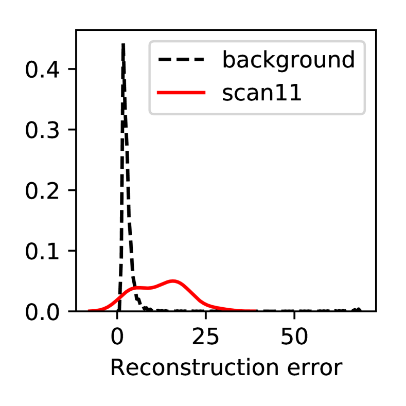
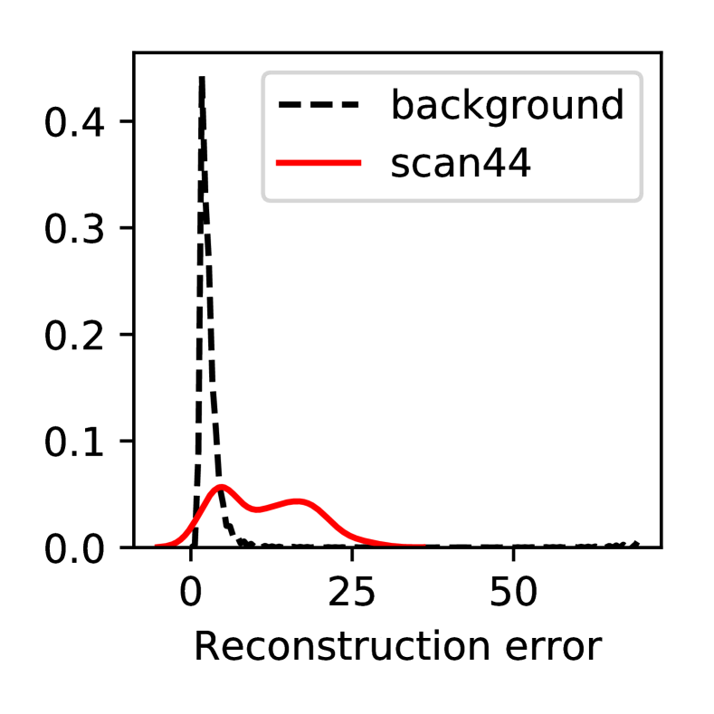
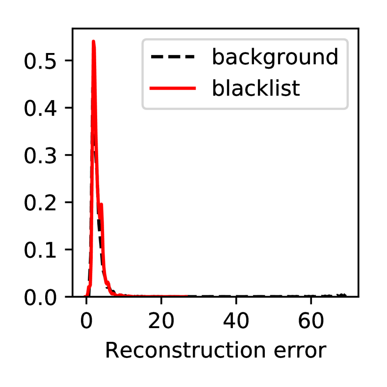
We present the distribution of the reconstruction errors for the training data on Fig. 2. The ground truth labels are used to separate the anomalies from the background flows, which let us examine whether the anomalies behave differently from the normal behaviors. Overall, there is some overlap with the background for spam, botnet, DoS, and scanning activities, but we can find a cut off point to roughly separate them. For blacklists, however, their behaviors are indistinguishable from the background traffic.
V-A Baseline
We compare our proposed anomaly detection framework GEE that uses VAE against that of AE and also a Gaussian Based Thresholding (GBT) approach. For a fair comparison, the baseline AE shares the same architecture as the VAE, and as illustrated in Fig. 1. The AE is implemented using Keras, a high level open source neural network library. We use the same TensorFlow backend for training the AE. This is by minimizing the reconstruction error (mean square error) using the stochastic optimizer Adam [37], with minibatch size chosen to be 256. Similar to the VAE, data points that have large reconstruction error are flagged as anomalies.
For the GBT, we fit independent but non-identical Gaussian distribution models to the features to learn the standard behaviors of the data. Then, we compute the Z-score for all features in the testing dataset and use the product of the average, standard deviation, and the maximum of the Z-scores as final score for anomaly detection. The data point with score that exceeds a certain threshold is considered as anomaly. We emphasize that both the AE and GBT are trained on the same extracted features as in VAE, this is to ensure the comparison is performed over the models rather than feature engineering.
V-B ROC Performance on Anomaly Detection
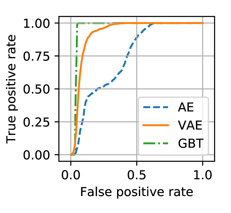
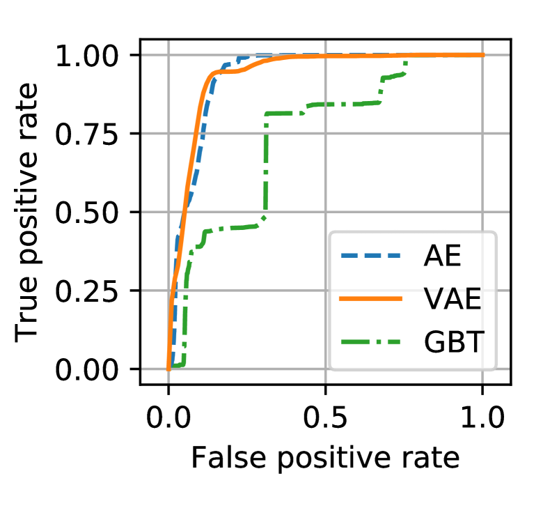
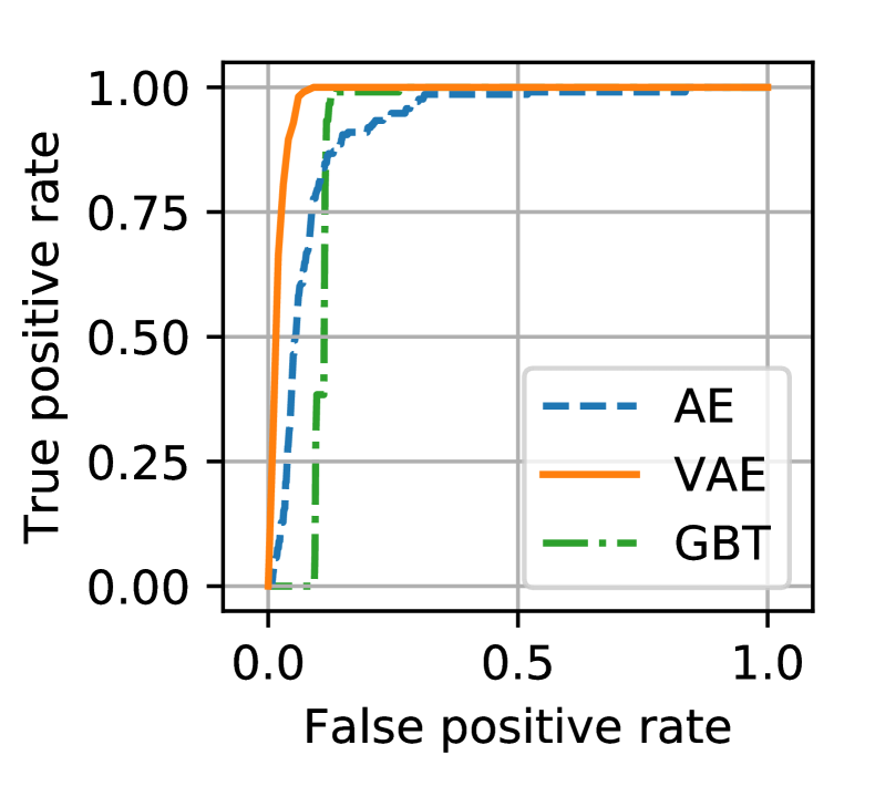
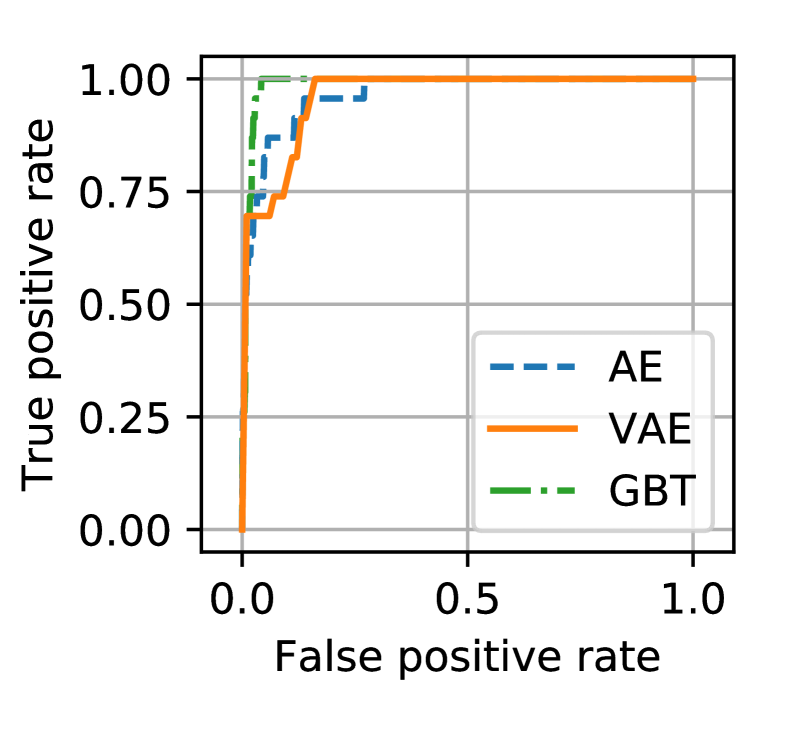
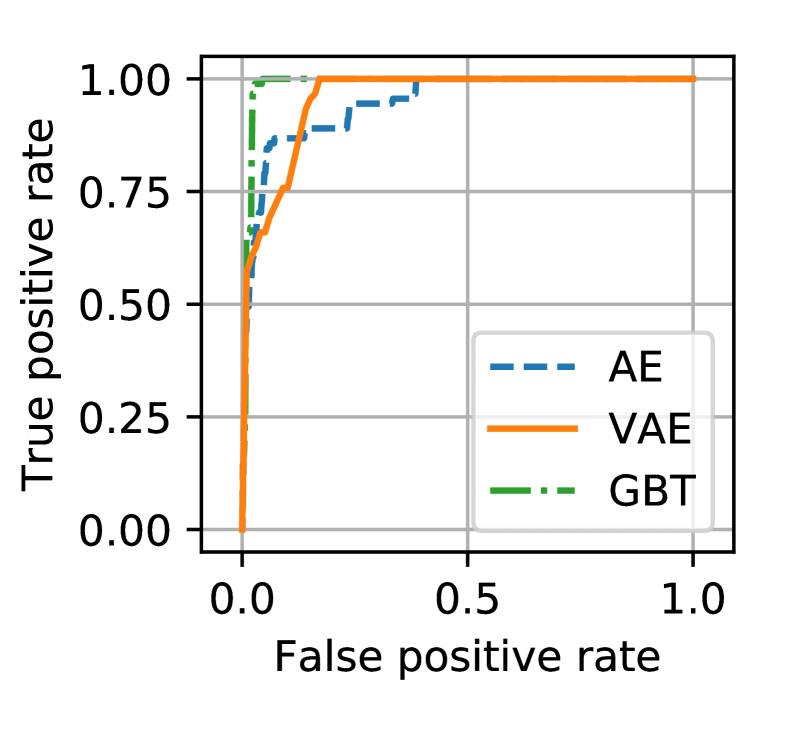
We evaluate the performance of these three methods (VAE, AE and GBT) using Receiver Operating Characteristic (ROC) curves, where the true positive rates are plotted against the false positive rates by varying the sensitivity or threshold for anomaly detection. A good performance is where the true positive is high while the false positive is low.
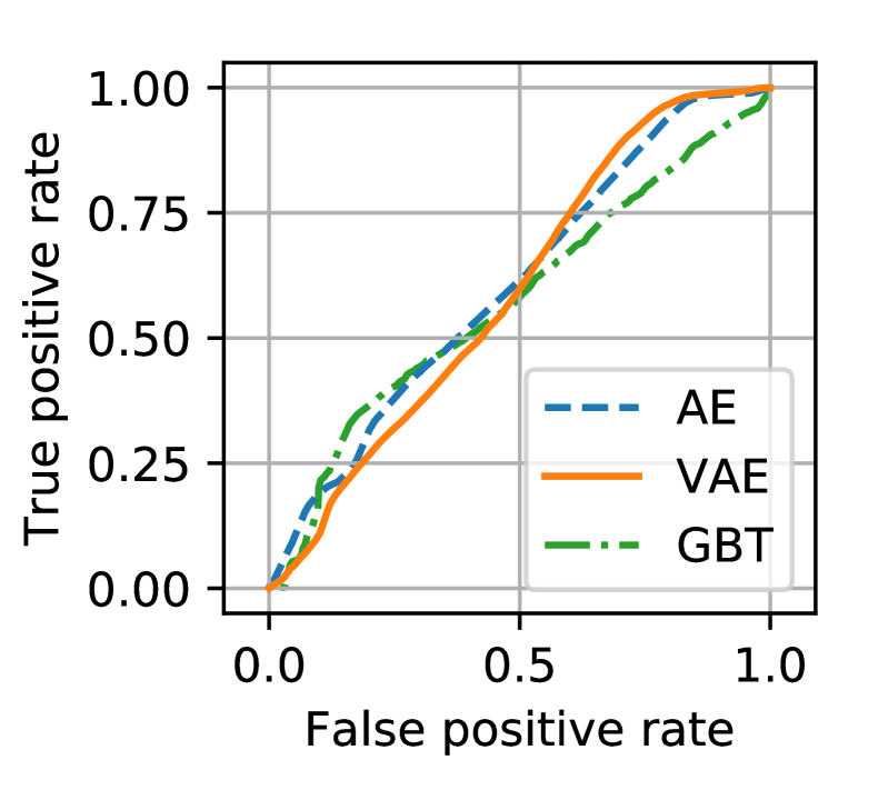
We plot the ROC results on the training dataset in Fig. 3 and on the testing dataset in Fig. 5. The results on the training data are presented because unlike supervised learning, the labeled data is not used for training, hence the results indicate how good the algorithms are in finding anomalies from statistics of the same day. On the other hand, results for the testing data evaluate on how the anomaly detection generalizes to a new day based on statistics from another day in the training data. For reference, we include the results for blacklisted IP addresses which clearly cannot be identified through the statistics from the NetFlow records, see Fig. 3(f).
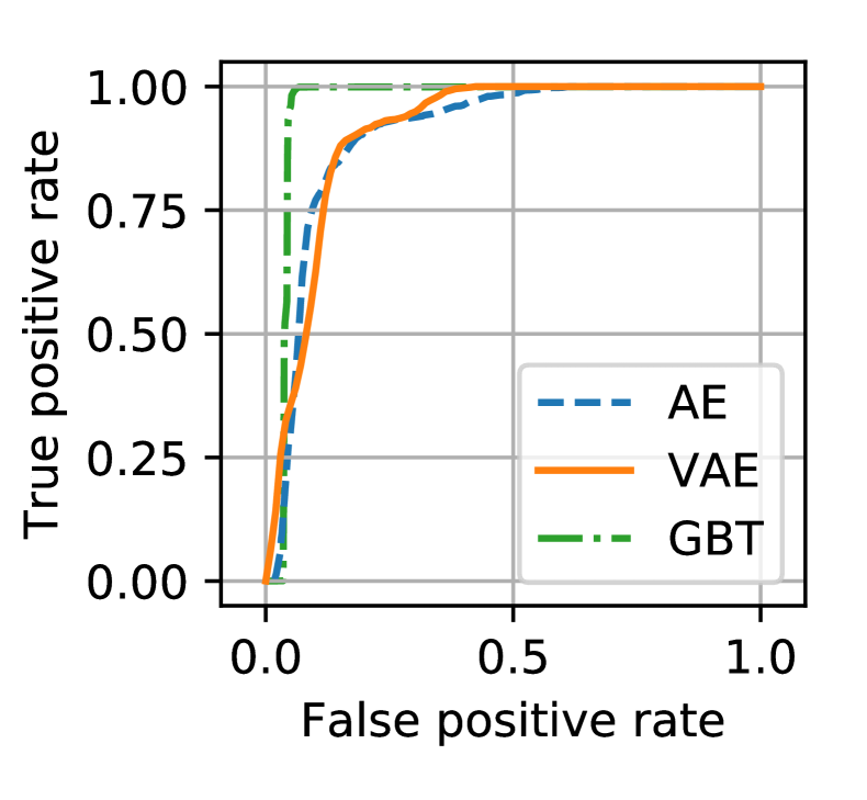
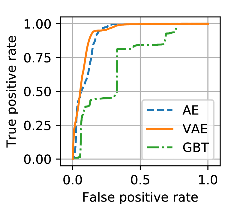
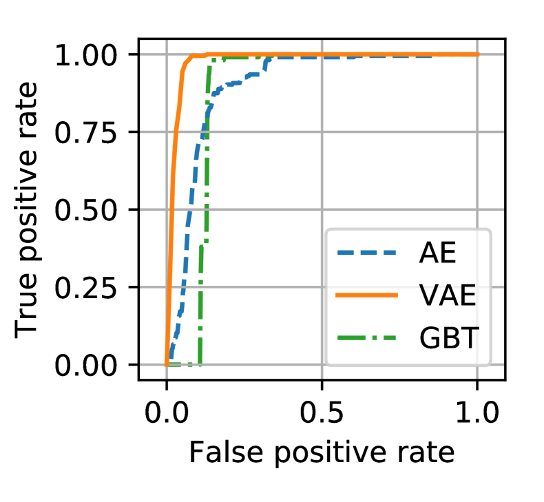
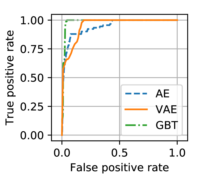
From the results, we make the following observations. First, threshold based approaches such as GBT work well for attacks that increase the volume of certain categories of traffic significantly, such as spam and port scanning. However, such approaches do not work as well for botnet and low rate DoS. On the other hand, AE does not work well for spam and low rate DoS. For these two attacks, AE may be unable to differentiate spam from regular email traffic because of the high volume, and unable to detect DoS due to the low rate. Overall, VAE is the most robust and has good performance on all attack types. Table II summarizes the individual and average area under the ROC curve (AUC) for various attacks (except blacklist) and detection models. Clearly, VAE has the best overall performance in terms of AUC. Note that the AUC results on the test set are aggregated over the different days, i.e., spam attacks are from March 18 and 20, while DoS, botnet, and port scanning attacks are originated from July 31.
| Model | DoS | BotNet | Scan11 | Scan44 | Spam | Average |
|---|---|---|---|---|---|---|
| Train | ||||||
| GBT | ||||||
| AE | ||||||
| VAE | 0.956 | |||||
| \hdashlineTest | ||||||
| GBT | ||||||
| AE | ||||||
| VAE | 0.947 | |||||
| \hdashlineF.print | 0.962 |
V-C Identifying and Using Gradient Fingerprints
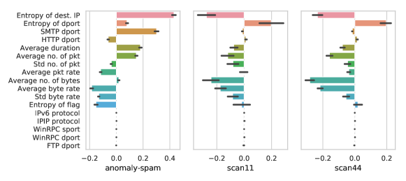
In this section, we compute and identify the gradients for all the features for various attacks. Fig. 4 shows the gradients of the features for spam, scan11, and scan44. Recall that 53 features are used as input to VAE and significant features with sufficient variation in gradients are shown in the figure. The black bars reflect one standard error for the gradients, which are useful for assessing the significance of the gradients, i.e., whether it is due to noise or not. We also present the features that are not significant for contrast. Note that similar gradient-based fingerprints are available for the other labeled attacks, not shown here due to space.
Based on the results, we can make the following observations. First, only a small subset of the features have large gradients. Second, these features with the greatest absolute gradients provide an explanation for why these flows of an IP are detected as anomalies. For example, in the case of spam attacks (which includes sending spam emails), five features have more positive gradient (higher than the learned normal) while four features have much negative gradient (lower than learned normal). Next, these combination of gradient and features can be used as a fingerprint to identify or cluster similar attacks. For example, it can be observed from Fig. 4 that Scan11 and Scan44 have similar gradient fingerprints.
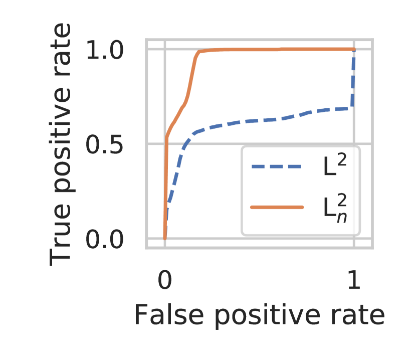
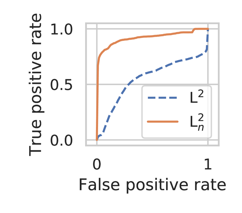
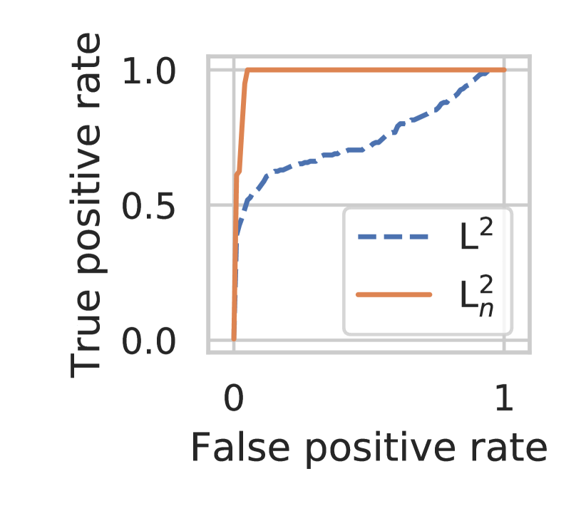
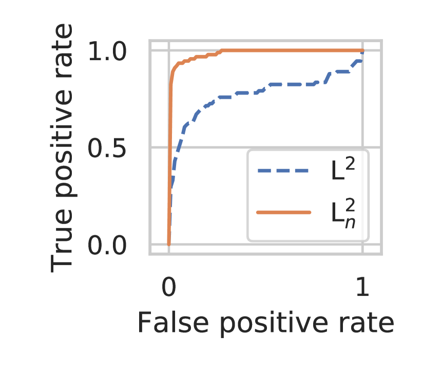
To further validate our claim that these gradient fingerprints are useful in identifying similar attacks, we plot the ROC for various attacks detected in the following way. First, let denote the Euclidean distance between the average gradient fingerprint obtained from data with labeled attacks and the gradients of the VAE’s objective function w.r.t. each test data point. Similarly, define as the same distance metric but computed on normalized gradient vectors. The ROC is then produced by varying the threshold on or distance. If the gradient fingerprint is a good measure of an attack, we expect the ROC to have high true positive and low false positive.
The results are shown in Fig. 6. It is encouraging to see that with the use of , the gradient fingerprints learned are indeed good representations of these attacks. In fact, it is an improvement upon using the reconstruction error for anomaly detection, see the last row on Table II for the its AUC. We also note that the result is slightly worse for botnet, see Fig. 6(b). This could be because there are many patterns behind the botnet anomalies. Hence, simply averaging all normalized gradients for botnet might not be the best approach.
Finally, we may also conclude that we have discovered a new attack if an unseen gradient fingerprint is identified.
V-D Clustering of Anomalies
Another possible use of the VAE generated gradients is that they can be used to cluster or group the different attacks. The idea is that if the clustering is effective, attacks should be limited to a relatively small number of clusters.
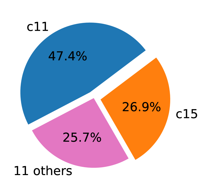
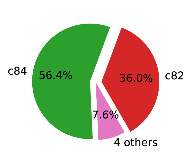
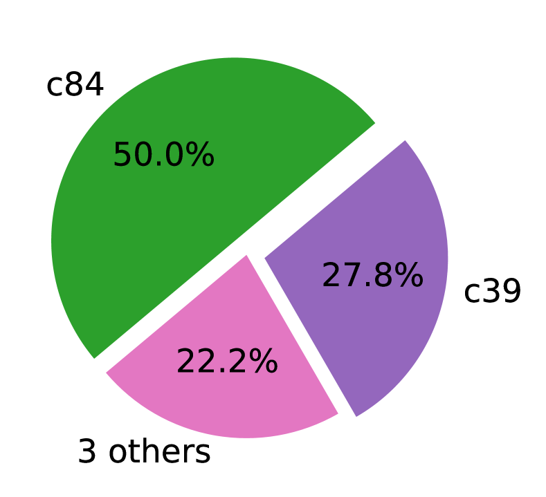
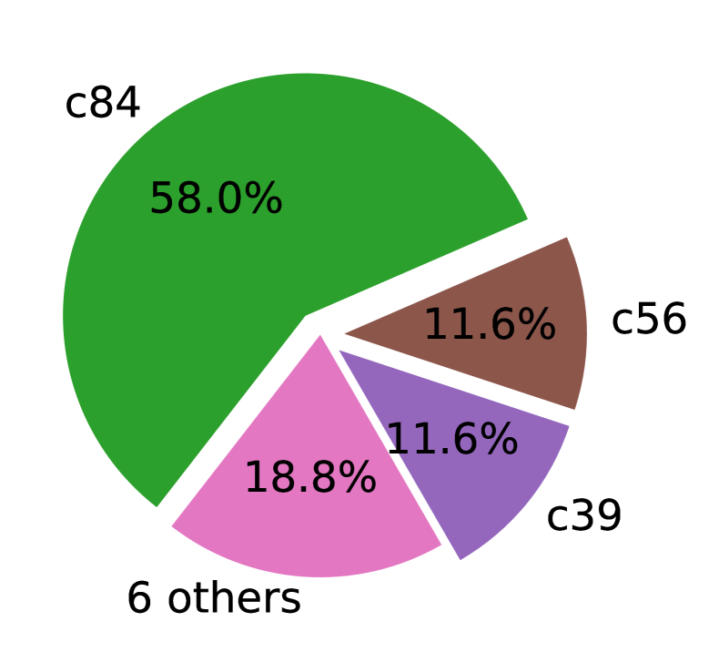
We performed k-mean clustering with random initial seed on the training dataset with . Fig. 7 illustrates the clusters associated with the attacks discussed above. We find that 92.4% of the DoS attacks appear only in two clusters (c82 and c84) with the other 7.6% appearing in four other clusters. For spam attacks, 74.3% of them appear in two clusters (c11 and c15), while 25.7% appears in another 11 clusters. This suggests that the attacks generally exhibit small number of main behavioral patterns and thus the analysts can focus on a small subset of clusters to study a particular type of attacks.
V-E Processing Overhead of VAE
Training of the VAE is performed on a single graphical processing unit (GPU) GTX 1080Ti with Intel Xeon CPU E5-2683 (16 cores, 2.1GHz), and 256Gb of RAM, which enables real time online training on streaming data. Since the features are aggregated into a 3-minute sliding window, the running statistics from the NetFlow records are kept for three minutes before discarded. On average, feature extraction took about 25 seconds for every 3-minute window of the UGR data, which corresponds to about 200k NetFlow records. Note that our implementation did not optimize for such operation, and speed improvement can easily be achieved.
Training using the TensorFlow framework is highly parallelizable and thus runs very quickly. For every minibatch of 300 data points of aggregated features, only 10ms is needed for training; while testing the data points for abnormality takes about 20ms. Hence, almost all the processing is due to the feature extraction. With the current setup, even without speeding up the feature extraction further, our algorithm can easily perform anomaly detection in real-time.
VI Conclusion
We proposed GEE, a VAE-based framework that is robust in detecting a variety of network based anomalies. We observed that the VAE performs better overall compared to the AE and a Gaussian based thresholding (GBT) method. Further, we demonstrated how to use the gradient information from the VAE to provide an explanation for the flagged anomalies. Also, the gradient-based fingerprints, when used directly for anomaly detection, was shown to achieve an overall better performance.
A potential future research is to use the conditional VAE (CVAE) [43] for anomaly detection. The CVAE was developed by the deep learning community as an extension of the VAE to allow for additional auxiliary labels that are available. With CVAE, one can consider training an anomaly detection system from multiple data sources that have different behaviors.
Acknowledgment
This research is supported by the National Research Foundation, Prime Minister’s Office, Singapore under its Corporate Laboratory@University Scheme, National University of Singapore, and Singapore Telecommunications Ltd.
References
- [1] Symantec, “Internet Security Threat Report,” 2018, https://www. symantec.com/content/dam/symantec/docs/reports/istr-23-2018-en.pdf; accessed July 2018.
- [2] M. Antonakakis, T. April, M. Bailey, M. Bernhard, E. Bursztein et al., “Understanding the Mirai botnet,” in Proc. 26th USENIX Security Symposium, 2017, pp. 1093–1110.
- [3] B. Claise, B. Trammell, and P. Aitken, “Specification of the IP flow information export (IPFIX) protocol for the exchange of flow information,” Internet Requests for Comments, RFC Editor, STD 77, 2013. [Online]. Available: http://www.rfc-editor.org/rfc/rfc7011.txt
- [4] A. Lakhina, M. Crovella, and C. Diot, “Characterization of network-wide anomalies in traffic flows,” in Proc. ACM SIGCOMM Conf. on Internet Measurement (IMC), 2004, pp. 201–206.
- [5] F. Silveira, C. Diot, N. Taft, and R. Govindan, “ASTUTE: Detecting a different class of traffic anomalies,” in Proc. ACM SIGCOMM, 2010, pp. 267–278.
- [6] J. Wang and I. C. Paschalidis, “Statistical traffic anomaly detection in time-varying communication networks,” IEEE Trans. on Control of Network Systems, vol. 2, no. 2, pp. 100–111, 2015.
- [7] R. Sommer and V. Paxson, “Outside the closed world: On using machine learning for network intrusion detection,” in Proc. IEEE Symposium on Security and Privacy, 2010, pp. 305–316.
- [8] G. Maciá-Fernández, J. Camacho, R. Magán-Carrión, P. García-Teodoro, and R. Therón, “UGR’16: A new dataset for the evaluation of cyclostationarity-based network IDSs,” Computers & Security, vol. 73, pp. 411–424, 2018.
- [9] N. Duffield, P. Haffner, B. Krishnamurthy, and H. Ringberg, “Rule-based anomaly detection on IP flows,” in Proc. IEEE INFOCOM, 2009, pp. 424–432.
- [10] Y. Gu, A. McCallum, and D. Towsley, “Detecting anomalies in network traffic using maximum entropy estimation,” in Proc. ACM IMC, 2005, pp. 345–350.
- [11] G. Nychis, V. Sekar, D. G. Andersen, H. Kim, and H. Zhang, “An empirical evaluation of entropy-based traffic anomaly detection,” in Proc. ACM IMC, 2008, pp. 151–156.
- [12] P. Barford, J. Kline, D. Plonka, and A. Ron, “A signal analysis of network traffic anomalies,” in Proc. ACM SIGCOMM Workshop on Internet Measurement (IMW), 2002, pp. 71–82.
- [13] F. Simmross-Wattenberg, J. I. Asensio-Perez, P. Casaseca-de-la Higuera et al., “Anomaly detection in network traffic based on statistical inference and alpha-stable modeling,” IEEE Trans. on Dependable and Secure Computing, vol. 8, no. 4, pp. 494–509, 2011.
- [14] I. Nevat, D. M. Divakaran, S. G. Nagarajan, P. Zhang, L. Su, L. L. Ko, and V. L. L. Thing, “Anomaly detection and attribution in networks with temporally correlated traffic,” IEEE/ACM Trans. on Networking, vol. 26, no. 1, pp. 131–144, 2018.
- [15] I. Paredes-Oliva, I. Castell-Uroz, P. Barlet-Ros, X. Dimitropoulos, and J. Solé-Pareta, “Practical anomaly detection based on classifying frequent traffic patterns,” in Proc. IEEE INFOCOM Workshops, 2012, pp. 49–54.
- [16] L. Bilge, D. Balzarotti, W. Robertson, E. Kirda, and C. Kruegel, “Disclosure: Detecting botnet command and control servers through large-scale NetFlow analysis,” in Proc. ACSAC, 2012, pp. 129–138.
- [17] A. Lakhina, M. Crovella, and C. Diot, “Diagnosing network-wide traffic anomalies,” SIGCOMM CCR., vol. 34, no. 4, pp. 219–230, 2004.
- [18] H. Ringberg, A. Soule, J. Rexford, and C. Diot, “Sensitivity of PCA for traffic anomaly detection,” SIGMETRICS Perform. Eval. Rev., vol. 35, no. 1, pp. 109–120, 2007.
- [19] D. Brauckhoff, K. Salamatian, and M. May, “Applying PCA for traffic anomaly detection: Problems and solutions,” in Proc. IEEE INFOCOM, 2009, pp. 2866–2870.
- [20] T. A. Tang, L. Mhamdi, D. McLernon, S. A. R. Zaidi, and M. Ghogho, “Deep learning approach for network intrusion detection in software defined networking,” in Wireless Networks and Mobile Communications (WINCOM). IEEE, 2016, pp. 258–263.
- [21] P. Torres, C. Catania, S. Garcia, and C. G. Garino, “An analysis of recurrent neural networks for botnet detection behavior,” in Biennial Congress of Argentina (ARGENCON). IEEE, 2016, pp. 1–6.
- [22] P. Baldi, “Autoencoders, unsupervised learning, and deep architectures,” in Proc. ICML Workshop on Unsupervised and Transfer Learning, 2012, pp. 37–49.
- [23] N. Shone, T. N. Ngoc, V. D. Phai, and Q. Shi, “A deep learning approach to network intrusion detection,” IEEE Transactions on Emerging Topics in Computational Intelligence, vol. 2, no. 1, pp. 41–50, 2018.
- [24] U. Fiore, F. Palmieri, A. Castiglione, and A. De Santis, “Network anomaly detection with the restricted Boltzmann machine,” Neurocomputing, vol. 122, pp. 13–23, 2013.
- [25] Y. Mirsky, T. Doitshman, Y. Elovici, and A. Shabtai, “Kitsune: An ensemble of autoencoders for online network intrusion detection,” arXiv preprint arXiv:1802.09089, 2018.
- [26] J. An and S. Cho, “Variational autoencoder based anomaly detection using reconstruction probability,” Special Lecture on IE, vol. 2, pp. 1–18, 2015.
- [27] S. Ren, K. He, R. Girshick, and J. Sun, “Faster R-CNN: Towards real-time object detection with region proposal networks,” in Advances in neural information processing systems, 2015, pp. 91–99.
- [28] A. Roy, J. Sun, R. Mahoney, L. Alonzi, S. Adams, and P. Beling, “Deep learning detecting fraud in credit card transactions,” in Systems and Information Engineering Design Symposium, 2018, pp. 129–134.
- [29] W.-N. Hsu, Y. Zhang, and J. Glass, “Unsupervised domain adaptation for robust speech recognition via variational autoencoder-based data augmentation,” in Automatic Speech Recognition and Understanding Workshop. IEEE, 2017, pp. 16–23.
- [30] M. Ancona, E. Ceolini, C. Öztireli, and M. Gross, “A unified view of gradient-based attribution methods for deep neural networks,” in International Conference on Learning Representations, 2018.
- [31] Y. Bengio, “Practical recommendations for gradient-based training of deep architectures,” in Neural Networks: Tricks of the Trade. Springer, 2012, pp. 437–478.
- [32] D. P. Kingma and M. Welling, “Auto-encoding variational Bayes,” arXiv preprint arXiv:1312.6114, 2013.
- [33] A. Jain, K. Nandakumar, and A. Ross, “Score normalization in multimodal biometric systems,” Pattern Recognition, vol. 38, no. 12, pp. 2270–2285, 2005.
- [34] M. Abadi, P. Barham, J. Chen, Z. Chen, A. Davis et al., “TensorFlow: A system for large-scale machine learning,” in Proc. Conference on Operating Systems Design and Implementation, 2016, pp. 265–283.
- [35] D. M. Blei, A. Kucukelbir, and J. D. McAuliffe, “Variational inference: A review for statisticians,” J. Amer. Statist. Assoc., vol. 112, no. 518, pp. 859–877, 2017.
- [36] A. G. Baydin, B. A. Pearlmutter, A. A. Radul, and J. M. Siskind, “Automatic differentiation in machine learning: A survey.” Journal of Machine Learning Research, vol. 18, no. 153, pp. 1–153, 2017.
- [37] D. P. Kingma and J. Ba, “Adam: A method for stochastic optimization,” in Third International Conference on Learning Representations, 2015.
- [38] DARPA Datasets, https://www.ll.mit.edu/ideval/docs/index.html.
- [39] A. Shiravi, H. Shiravi, M. Tavallaee, and A. A. Ghorbani, “Toward developing a systematic approach to generate benchmark datasets for intrusion detection,” Comp. & Sec., vol. 31, no. 3, pp. 357–374, 2012.
- [40] N. Moustafa and J. Slay, “UNSW-NB15: A comprehensive data set for network intrusion detection systems (UNSW-NB15 network data set),” in Military Communications and Info. Sys. Conf. IEEE, 2015, pp. 1–6.
- [41] S. Garcia, M. Grill, J. Stiborek, and A. Zunino, “An empirical comparison of botnet detection methods,” Comp. & Sec., vol. 45, pp. 100–123, 2014.
- [42] MAWI Working Group Traffic Archive, http://mawi.wide.ad.jp/mawi.
- [43] K. Sohn, H. Lee, and X. Yan, “Learning structured output representation using deep conditional generative models,” in Advances in Neural Information Processing Systems, 2015, pp. 3483–3491.