On Axion Reheating in the String Landscape
Abstract
We demonstrate that asymmetric reheating arises in a large ensemble of string compactifications with many axions and gauged dark sectors. This phenomenon may help avoid numerous cosmological problems that may arise if the sectors were reheated democratically. Distributions of couplings are presented for two classes of axion reheatons, both of which exhibit very small couplings to most of the gauge sectors. In one class, ratios of reheating couplings and also preferred gauge groups are frequently determined by local regions in the string geometry.
I Introduction
An inflationary epoch in the early universe provides solutions to the monopole, horizon, and flatness problems Guth (1981); Linde (1982). During the exponential expansion of space caused by inflation, energy stored in fields other than the inflaton is quickly diluted, requiring a transfer of energy to Standard Model particles at the end of inflation, known as reheating Abbott et al. (1982); Dolgov and Linde (1982); Albrecht et al. (1982); Kofman et al. (1994); Shtanov et al. (1995). More generally, scalar fields other than the inflaton could be responsible for reheating; henceforth, we refer to this field as the reheaton. There are many models of reheating, as well as non-perturbative generalizations such as preheating Traschen and Brandenberger (1990); Kofman et al. (1994); Adshead et al. (2015); Garcia-Bellido and Linde (1998); Cuissa and Figueroa (2018). Crucial to all are the couplings of the reheaton to the visible sector, as well as potential dark sectors. However, reheating of dark sectors can lead to cosmological issues, such as the overproduction of glueball dark matter Halverson et al. (2017a, 2018a), which may often be exacerbated in the presence of many gauged dark sectors. The problem can be partially ameliorated if the reheaton couples more to some sectors than others; i.e., if reheating is asymmetric (see, e.g., Kolb et al. (1985); Berezhiani et al. (1996); Adshead et al. (2016)).
It has long been known that string theory gives rise to gauged dark sectors (see, e.g., Gross et al. (1985); Lerche et al. (1987)), but in recent years their degree of relevance has strengthened significantly. For instance, the F-theory Vafa (1996); Morrison and Vafa (1996) geometry with flux vacua Taylor and Wang (2015) and the exact ensemble Halverson et al. (2017b) of F-theory geometries exhibit and and gauged dark sectors, respectively. Together with Taylor and Wang (2018), these comprise perhaps the largest known concrete regions of the landscape of string vacua, and they motivate cosmologies with large numbers of gauge sectors and axions.111When we refer to axions, we mean not only the pseudoscalars arising from string compactification that couple to the gauge sectors, but also more general axion-like particles. Details of those cosmologies, and in particular whether they are realistic, depend crucially on reheating.
We initiate a study of reheating in these constructions, focusing on the case of axion reheating. We will calculate the couplings of axions to the various gauge sectors in the geometries of Taylor and Wang (2015) and Halverson et al. (2017b); the former is known as , and the latter is known as the Tree ensemble. We will demonstrate that axions that couple significantly to only a few gauge sectors arise naturally in the ensemble, giving rise to asymmetric reheating. We will show that such hierarchies often arise from local patches in the string geometry. Specifically, in the case that the axion reheaton is defined to be oriented along a gauge direction, we show that the sectors that are reheated to the highest temperatures are that gauge direction, and also gauge sectors that intersect this sector; for fixed axion reheaton and Calabi-Yau, the other gauge sectors are reheated to a universal temperature. For axion reheatons that are random combinations of gauge-direction axions, we still find asymmetric reheating, but to a lesser degree. We also explain how this geometric result could be extended to a larger region of the string landscape.
While there has been some significant progress in understanding reheating in string theory (see e.g. Kofman and Yi (2005); Cicoli and Mazumdar (2010); Blumenhagen and Plauschinn (2014)), there are important distinctions from the present work. For instance, previous works have sometimes been limited to a few examples, and (more importantly) all in the case where the number of fields and gauge sectors is relatively small. In contrast, we study over a thousand geometries drawn from the Tree ensemble. The average number of gauge sectors is ; this differs from the previously stated number of due to a truncation made for computational reasons. We also study reheating on . For a third regime of interest, the reheaton could also arise from the open string sector. Asymmetric reheating may also arise there, likely due to symmetries that charge open strings and therefore bias some sectors over others. On the other hand, for an inflaton reheaton, these models are more likely to give rise to an -problem that spoils slow-roll, which the axion case avoids due its shift symmetry. We leave a study of open string reheatons in these ensembles to future work.
This paper is organized as follows. In Section II we present effective field theories of axion reheating and their realization in F-theory. In Section III we compute distributions of reheating ratios in the Tree ensemble, and also in the F-theory geometry with the most flux vacua. In Section IV we study which gauge groups are most likely to be reheated under various assumptions. In Section V we summarize our results and discuss further aspects of the cosmology.
II Effective Field Theory
for Axion Reheating
We will consider an effective theory of axions and gauge sectors with field strengths in F-theory, where the index runs over the various gauge groups. The general, canonically-normalized, two-derivative effective Lagrangian takes the form
| (1) |
where and is the non-perturbative axion potential. We leave all traces implicit.
Let us consider a candidate axion reheaton . Our goal is to compute the couplings of to the various gauge sectors. In general there are many possibilities for and the one that is realized cosmologically is determined by inflationary dynamics. We will therefore address a simpler, but important question: if we can select a in order to attempt to reheat a single gauge sector , how much does necessarily couple to other gauge sectors? What is the distribution of those couplings? In answering this question, we will uncover a general geometric result which can be applied to more general cases. We consider a reheaton directed along the -th gauge direction. We can in general write the axion-gauge boson interactions as
| (2) |
where are unit vectors. Our candidate reheaton is then . In this case we will say that is oriented along . Clearly couples to , but in general will appear in the second sum in Eq. II (which we might not expect, a priori), and will therefore couple to other gauge groups, as well. Schematically, the effective interaction Lagrangian can be expanded as
| (3) |
where we have only retained the axion-dependance in Eq. 3. Our goal is then to compute the relative coupling strengths of to and with , given by and , respectively. From Eq. II we can see that . To read off , the coupling of to another other gauge group , we perform an basis transformation , such that , and then expand Eq. II in that basis. We then see that . We will focus on the ratio of the couplings , and we therefore define the quantity of interest as
| (4) |
We will explore these couplings in F-theory, and uncover some interesting structure.
Let us now consider the data of such EFTs derived from F-theory. We will view these as IIb compactified on a Kähler threefold , with generalized 7-branes. After stabilizing complex structure moduli, the light degrees of freedom of the effective field theory are gravity, gauge sectors, and Kähler moduli. The latter are written as:
| (5) |
where the are a basis of divisors on , is the Kähler form on , and is the Ramond-Ramond four-form gauge potential. The are volume moduli, which parametrize divisor volumes in , while the are the associated axions. With fixed volume moduli, the effective Lagrangian for the axions and gauge fields contains the terms
| (6) |
The tree-level Kähler potential for the Kähler moduli is written as
| (7) |
Here is the volume of computed with the Kähler form , where is a basis for :
| (8) |
The are the triple intersection numbers of divisors. Eq. 7 is known to receive corrections in both and the string coupling . As F-theory generically contains 7-branes with regions Halverson (2017), such corrections are not well understood in F-theory, so we will take Eq. 7 as a model for the Kähler potential.
The metric for the Kähler moduli then takes the form (for a derivation, see, e.g., Halverson et al. (2017c))
| (9) |
where is the inverse of . The inverse Kähler metric will play an important role in our analysis, and takes the form
| (10) |
The couplings of the axions to the gauge bosons, given by the in Eq. II, are determined by the wrappings of 7-branes on divisors: a 7-brane which carries a gauge sector and wraps a divisor couples to the linear combination of axions .
Let us express , , and in terms of the geometric basis . The kinetic term shown in Eq. (II) for the axion fields can be brought to the canonical form in Eq. (II) by diagonalizing the Kähler metric . Being symmetric and positive-definite, it can be decomposed as the matrix product , with orthogonal and diagonal. Thus, the relation follows. Plugging this into Eq. (II) and canonically normalizing the gauge fields, we can see that the dot products in Eq. 4 can be computed as
| (11) |
where
| (12) |
The division by the volume factor in Eq. 12 is a result of the canonical normalization of the gauge fields. It is interesting to note that the are invariant under the Kähler parameter scaling , , as the scale with weight , due to the in the denominator of Eq. 12, and scales with weight . This implies that the are only functions of the angular coordinates in the Kähler cone, or the cone in which all curves in have positive volume. It is convenient to define the variables as
| (13) |
We can then write
| (14) |
and
| (15) |
and therefore
| (16) |
Our goal will be to compute in an ensemble of F-theoretic examples.
Let us briefly comment on the potential for the axions. As mentioned above, the axions enjoy a continuous shift symmetry to all orders in perturbation theory, which is broken to a discrete shift symmetry by non-perturbative effects. As we will explain in the next section, the theories we will consider have large numbers of axions and condensing gauge sectors, whose low-energy dynamics will frequently result in gaugino condensates. The non-perturbative superpotential for the axions takes the schematic form
| (17) |
where and the ’s are constants, and the are the wrapping numbers of the 7-branes generating the gaugino condensates, with dual Coxeter numbers . There can also be stringy ED3-instantons that do not correspond to gauge theory instantons (see, e.g., the review Blumenhagen et al. (2009)), in which case . The superpotential in Eq. 17, the Kähler potential in Eq. 7, and its derivatives enter the supergravity potential to form the axion potential . Importantly, the axion masses are exponentially sensitive to the vacuum expectation values (vevs) of the Kähler moduli, and therefore to ensure that there exists an axion that can reheat the Standard Model to the required temperature, we need to ensure there is an axion whose corresponding saxion expectation value is not too large. We will later argue we always have at least one such axion. We will now review the construction and geometry of the largest-known explicit ensemble of F-theory geometries, known as the tree ensemble.
II.1 The Tree ensemble
The Tree ensemble is an ensemble of extra-dimensional geometries suitable for F-theory compactifications. They are toric bases that are generated by blowups of toric subvarieties on two particularly rich weak Fano toric threefolds, and form a connected network of geometries Carifio et al. (2018). Such blowups are expected to provide reasonable F-theory compactifications as they are finite distance in moduli space Hayakawa (1995); lung Wang (1997); Grassi (1991) from well-understood geometries that have weak coupling limits. Each base is topologically distance, and while the ensemble itself is much too large for a brute force scan, a detailed study of the construction algorithm of such bases yields universal results in the physics. In particular, virtually all the bases have large gauge sectors and many axions. An analytic proof shows that to high probability , the minimal gauge algebra on each geometry is , where is a model-dependent gauge algebra, and the depend on the ray structure of the toric fan. An even stronger result is obtained by taking random samples from the ensemble: the average number of gauge factors is , and the average rank of the gauge group is . The gauge sectors correspond to so-called non-Higgsable clusters Morrison and Taylor (2012a, b); Grassi et al. (2015); Morrison and Taylor (2015); Halverson and Taylor (2015); Taylor and Wang (2016); Halverson et al. (2017b); Taylor and Wang (2018), whose gauge group cannot be Higgsed geometrically, i.e., via brane splitting. While additional gauge groups can be further tuned, we will mainly focus on non-Higgsable gauge groups, as they require no tuning whatsoever. However, one should note that a tuned three-family MSSM (albeit with an undetermined number of Higgs pairs) arises ubiquitously on the one of the weak Fano toric threefolds Cvetic et al. (2019). An overwhelming fraction of these geometries contain inherently strongly-coupled 7-branes Halverson et al. (2018b). In the absence of flux these sectors do not have matter, and thus will confine, producing glueballs at low energies.
Let us briefly review the essential geometry of the Tree ensemble. Due to its toric nature the tree ensemble is combinatorial. A smooth weak Fano toric threefold, which is the starting point for our ensemble, is associated to a fine regular triangulation of a 3d reflexive polytope . Such a defines a fan . Toric blowups correspond to adding “exceptional” rays to and subdividing its cones. The blowup procedure terminates when the exceptional rays reach a certain distance from the boundary of , as the sufficient condition to be at finite distance in moduli space is violated; see Halverson et al. (2017b) for further details, and Halverson and Langacker (2018) for a lengthy introduction to the ensemble. Such a procedure has been informally coined as “adding a tree”, as the exceptional rays look like a tree above . Toric points correspond to triangles in , and toric curves to edges, and both admit tree structures above them by adding rays above the corresponding edge or triangle. Each additional ray added provides an additional axion to the EFT, and adding higher and higher trees forces more and larger gauge groups.
III Asymmetric reheating
from local couplings
In order to compute a large number of examples in a reasonable amount of time, we restrict ourselves to geometries with axions. We will find that this is sufficient to recognize a general pattern in the coupling ratios, and we will demonstrate how the behavior scales with the number of axions. This provides evidence that our results also hold in the bulk of the ensemble. To truncate the ensemble to a manageable number of axions, we only allow trees over of ten toric points. We consider geometries drawn from the Tree ensemble (this particular number was determined by running the geometric analysis on our cluster for 24 hours). Each geometry consists of random trees added over ten random toric points. The number of axions ranges from 139 to 213, with the average number of axions being 188. The number of gauge groups range from 57 to 78, with an average number of 75. The rank of the gauge groups ranged from 194 to 352, with an average value of 315.
The couplings are functions of the volume moduli, and their values therefore depend on details of moduli stabilization. Moduli stabilization is intricate with even a few moduli Cicoli et al. (2008), and often requires balancing terms the perturbative Kähler potential against the non-perturbative superpotential in a delicate fashion. Given that these corrections are not well-understood in F-theory, and are only computed to low-order in string theory Berg et al. (2005a, b), we will instead make the assumption that the volume moduli are stabilized in a region where certain non-perturbative effects may be safely neglected. For instance, there are known non-perturbative corrections to the Kähler potential, such as worldsheet instantons that contribute schematically as
| (18) |
where is a two-cycle. Therefore, as a proxy for control of the non-perturbative corrections in , we enforce that for all curves . This region was defined in Demirtas et al. (2018) as the stretched Kähler cone.222The stretched Kähler cone is not technically a cone, but instead a subregion within the Kähler cone at a fixed distance from the walls.
III.1 Sampling the Kähler cone
In Demirtas et al. (2018) it was shown that toric fourfolds and their anticanonical hypersurfaces typically have very narrow Kähler cones, forcing some four-cycle volumes to be large and some axions nearly massless if one demands stabilization in the stretched Kähler cone for reasons of control. We find the same structure for our toric threefolds. As a measure for the opening angle of the Kähler cone, we compute , defined by
| (19) |
Here the are the generators of the Mori cone, dual to the Kähler cone. In our ensemble these values range from to , with a mean of . This suggests that the angular space of the Mori cone is quite wide, and therefore the angular space of the Kähler cone is quite narrow. We therefore do not expect much variation in the physics as we change the angle, while remaining in the stretched Kähler cone.
To demonstrate this, we select the geometry with the largest and sample the stretched Kähler cone via random walks. To begin such a walk, we use Mathematica’s FindInstance method to find an initial point. While the inner workings of this method are not directly available to us, we find that this initial point has a large number of toric curves with area, and we therefore informally refer to this initial point as the apex of the stretched Kähler cone. We initiate the random walks from multiple starting points, beginning with the apex , and then scaling outward to , with . We consider unit length step sizes, measured with respect to the toric curves areas. The direction of the step is drawn from a normal distribution centered at zero, with variance . Allowing for steps in each random walk, we restrict ourselves to remain within the stretched Kähler cone by requiring all curves to have volume greater than or equal to unity. As we are aiming to sample the angular space of the stretched Kähler cone, we scale each point to a constant volume slice at the end of the random walk. For each scaled point we compute the mean fractional difference (MFD) for the four cycles with respect to starting point of the random walk , given by
| (20) |
We find a maximum MFD of , which implies the maximum average deviation of the four-cycle volumes is approximately . Given the small amount of volume variation in this region, and the fact that the axion-gauge field couplings are invariant under , , for the purposes of reading off generic physics in the stretched Kähler cone we find it sufficient to examine the apex.
III.2 Results of the scan
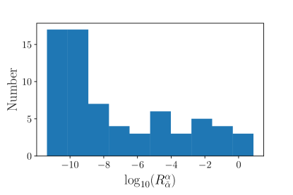
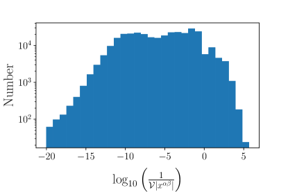
We compute the ratios in our ensemble of tree geometries. Let us first consider a single choice of in a single geometry. We show the distribution for in this example in Fig. 1. In this example there are a few sectors that couple to the reheaton on the same order as the coupling to , while the rest of the couplings are significantly smaller by many orders of magnitude. This observation is in fact general throughout our ensemble.
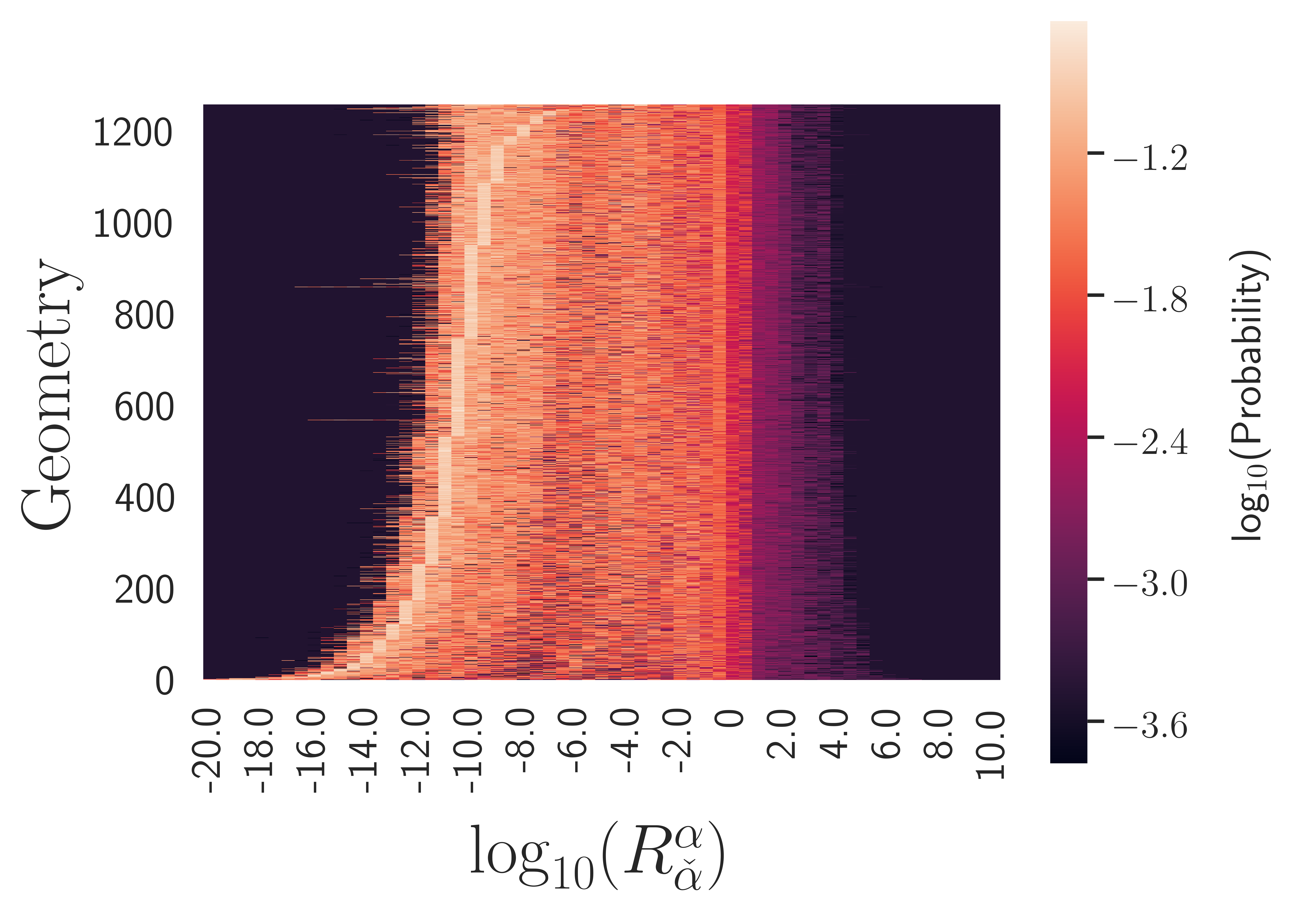
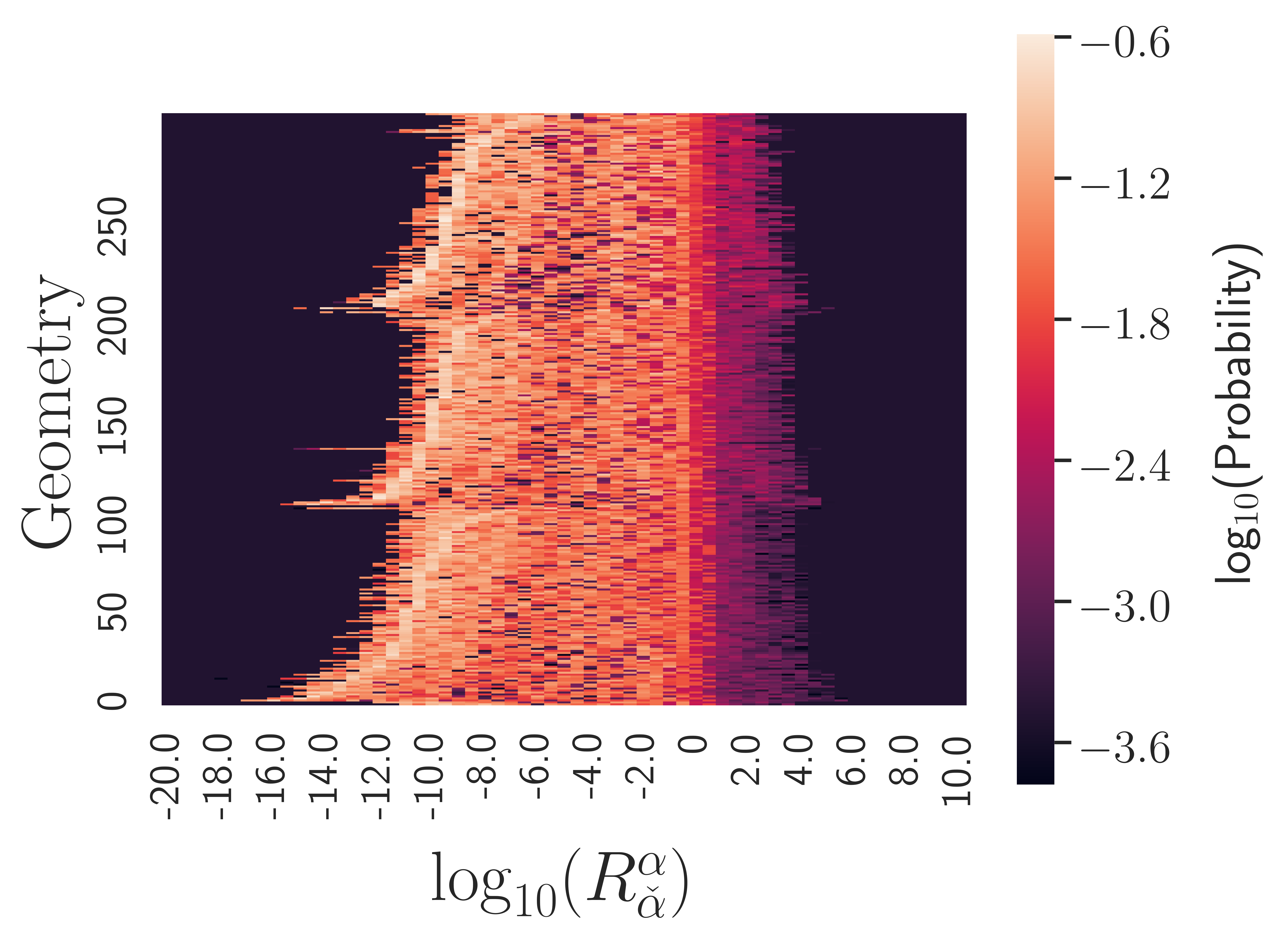
We plot the bulk results from all the geometries in our scan in a heat map, shown in Fig. 2. Specifically, each horizontal line in the heat map is a single geometry, and for each choice of gauge-oriented reheaton we compute for all other gauge sectors . The heat distribution is then probability to find a given .
The first notable feature of these distributions is that the peak of a typical distribution is around , which suggests that, given a reheaton oriented along a gauge group , the relative strength of the couplings of to other gauge sectors is usually negligible, down by over ten orders of magnitude. However, there is a tail towards larger values. From the right tail we can see that the fraction of is , and that these ratios extend to even larger values, reaching into . In these cases, even though one attempts to arrange for a reheaton to reheat a particular sector, necessarily couples to other sectors with much stronger coupling. The conclusion is that for a chosen to be oriented in a gauge direction, it will couple very weakly to most of the gauge sectors in the compactification (recall there are on average), but will couple non-trivially to a few.333This result will soon be discussed in light of common expectations about democratic reheating due to global closed string effects. This feature is what we call asymmetric reheating.
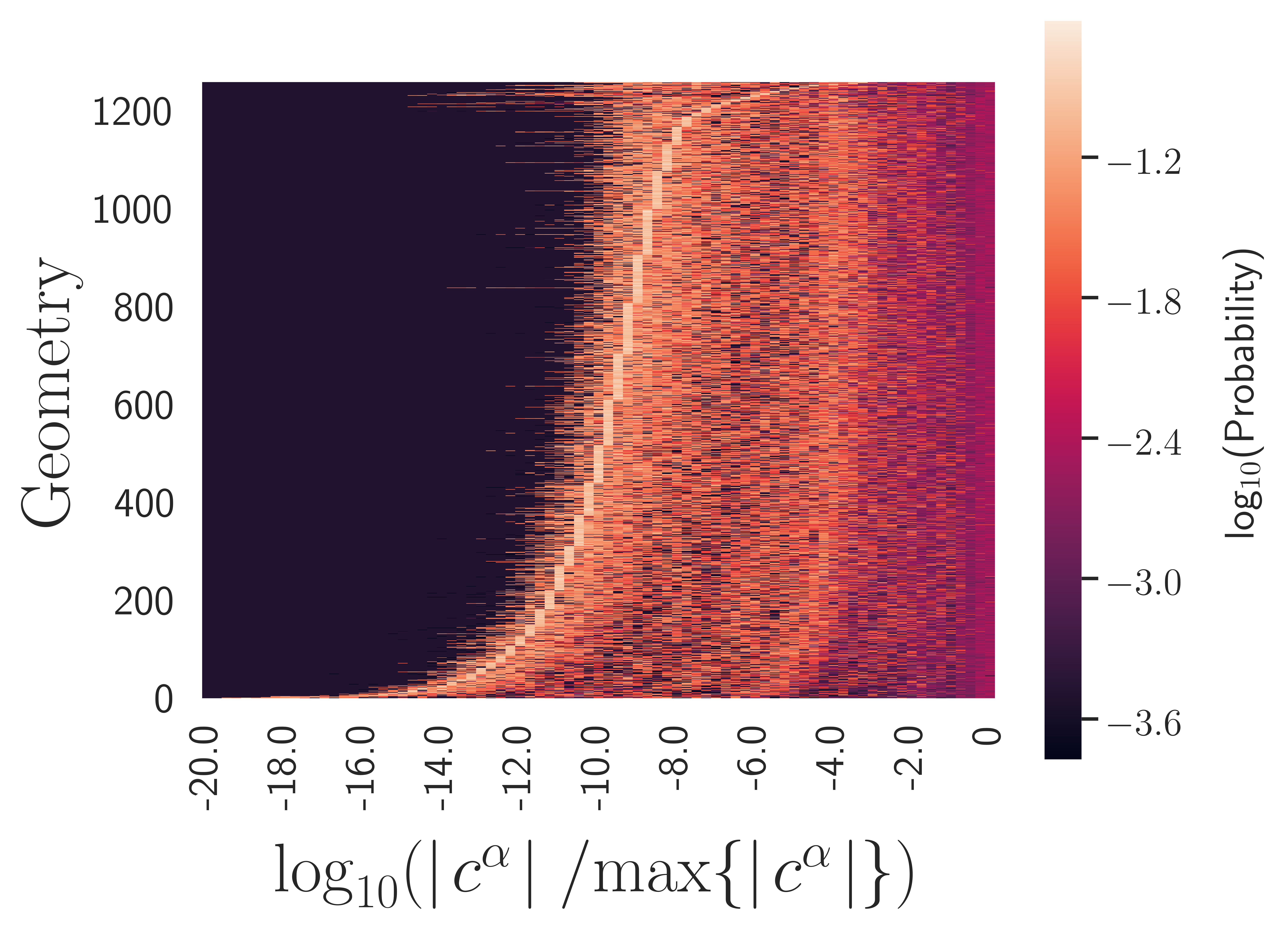
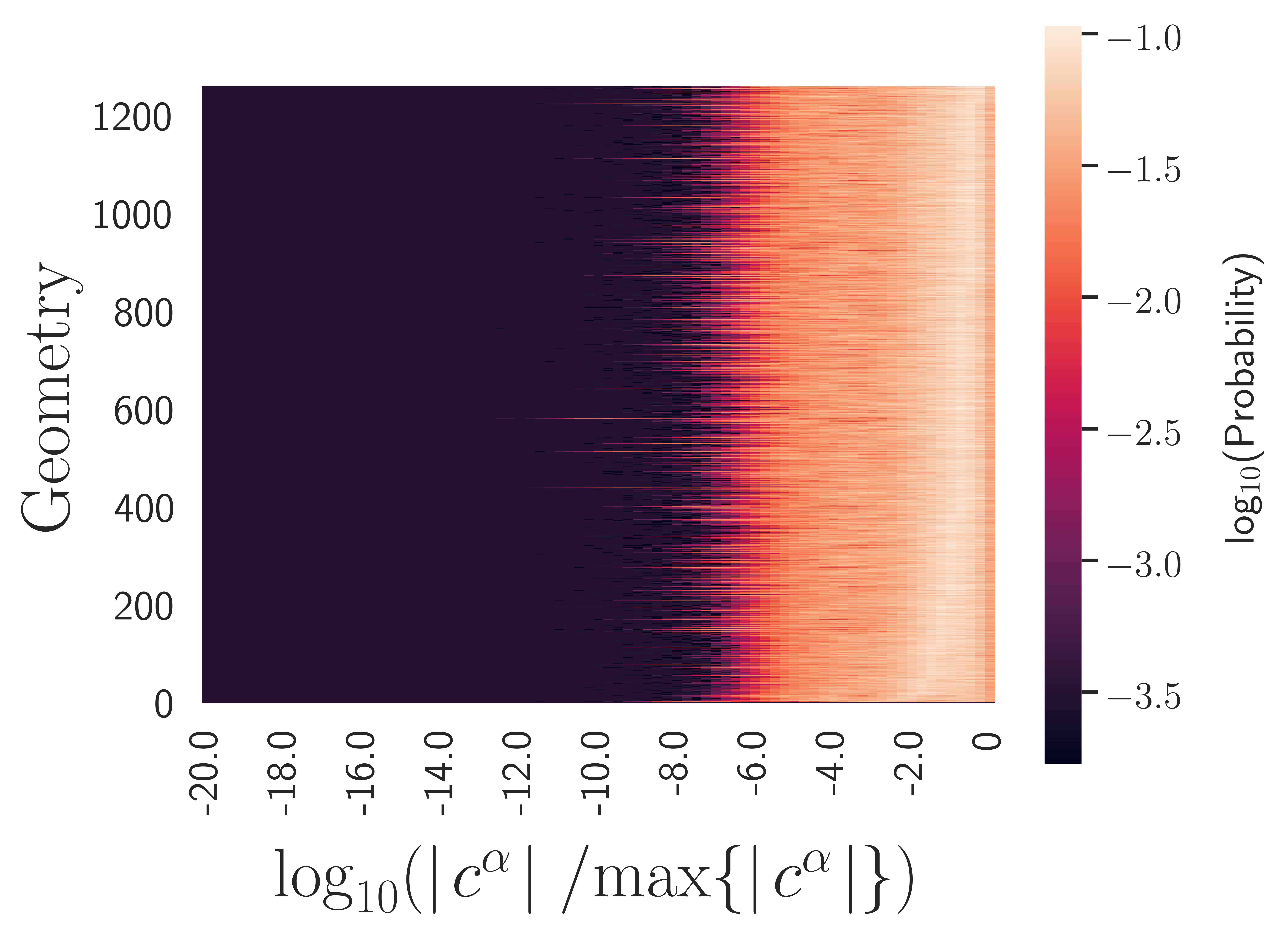
The above data captures the necessary minimal couplings of an axion reheaton, oriented along a single gauge direction, to other gauge sectors. However, cosmological dynamics could select other reheaton directions, and we should therefore contrast to another limiting point: random reheaton directions. In order to compare to more general reheaton directions, we consider the quantity , as is not well-defined if does not correspond to a single gauge direction. To generate such random directions, we draw the entries of from a normal distribution centered around zero, with variance . In the right hand side of Fig. 3 we plot the base-10 logarithm of for random axion-reheaton directions. Each horizontal line in the plot is a single geometry, and the heat distribution is the base-10 logarithm of the probability to find a given . In the left hand side of the same figure we also show from the gauge directions to contrast with the random directions.
We find that the couplings from the random directions are much less asymmetric that the oriented ones: the peak of the distribution for random reheatons on the right-hand side of Figure 3 is close to and has probability , indicating couplings to about of the gauge sectors. This should be contrasted to the left-hand side, the distribution for gauge-direction reheatons, where we see that the probability of an coupling is , indicating couplings to about of the gauge sectors. This result for random reheatons is consistent with expectations from effective field theory.
Another useful comparison arises from considering a random effective field theory of -axions, with a Lagrangian of the form given in Eq. II. We draw the entries of from a Wishart distribution, constructed from a normal distribution centered around zero, with variance . In addition, the matrix is taken as random with entries drawn from (i) a normal distribution centered around zero, with variance , (ii) random integers or (iii) sparse random integers. In all three cases, the result is a distribution similar to the one shown in Fig. 3 (right), but with significantly larger entries: the peaks of the distributions are closer to unity. This indicates that a generic random EFT clearly differs from the random reheaton direction studied above.
In summary, we conclude that some degree of asymmetric reheating is generic in this string ensemble. The extent to which the reheating is asymmetric is determined by how much a reheaton is aligned with a gauge eigenstate direction vs. a random combination of those directions. In the former case, we see couplings to of the gauge sectors, and in the latter case we see couplings to of the gauge sectors. Given a large number (e.g. , as here) of gauge sectors, one expects that obtaining a realistic cosmology requires some degree of asymmetric reheating. Our results demonstrate that models of axion reheating can potentially give rise to realistic cosmologies via asymmetric reheating, particularly in the case that the reheaton is aligned along a single gauge group.
III.3 Geometric origin of asymmetric reheating
Let us now discuss the origin of this hierarchy of couplings that lead to asymmetric reheating. Recall the definition of , given in Eq. 16. The numerator and denominator each have a local piece that depends on the intersection of () and , given by their respective , as well as a non-local additive factor of . A priori it is not clear which piece, if either, should dominate; for instance both have the same volume scaling under . However, we find that the approximation
| (21) |
is highly accurate first-order approximation; that is, when , only the local pieces matter when and intersect, and the couplings are highly suppressed when they do not.
We arrived at this conclusion by an analysis of using a neural network444Neural networks are excellent function approximators, and are central to recent efforts to study the string landscape using machine learning; see, e.g., He (2017); Ruehle (2017); Carifio et al. (2017). using a strategy that we will call input-dropout. The goal of this analysis is to understand which variables are critical in predicting , as well as to potentially discover correlations between such variables. Our network is a fully connected feed-forward neural network implemented in PyTorch, with five layers, each with width 100. We initially trained the network to predict given several input variables, which were the gauge group reheaton, the additional gauge groups, the graph distance between the various divisors (defined with respect to the toric fan), the overall volume of , the volumes of all toric divisors, as well as the volume combinations (which is enough to implicitly determine the areas of the toric curves as well). These additional input variables were included since they might provide an alternative understanding of .
After training for 10 epochs, the mean squared error loss was , indicating very accurate predictions. However, often only a subset of the input variables are important for accurately predicting the output, and this can be tested in a simple way by input-dropout: systematically removing some of the inputs and checking whether the neural network still makes accurate predictions. Removing all of the variables except , we see that the network still predicts with a mean squared error loss of after training for 10 epochs. By contrast, if those input variables are removed and all others are left intact, the network only predicts with mean squared error loss of after the same number of epochs. This large jump in mean square error loss suggests that any additional interesting or surprising correlations that could determine are intricate, and if present may require machinery beyond a simple neural net to uncover.
We therefore have the highly accurate approximation
| (22) |
In retrospect, this result could have been derived instead by simply looking at the distribution of presented in Fig. 4, from which one concludes that the contribution is often negligible compared to that of . However, from Fig. 4 we see that this approximation breaks down in about of the cases. Let us analyze the behavior in the regime of greatest interest, when the is significant (). Here we find that in of the cases when , respectively, allowing us to approximate the numerator by . Expanding the denominator to leading order in , we have
| (23) |
which corrects the local picture (21). To know how robust the local picture is, we would like to compute the size of the correcting factor. We find that in of the cases with , which leads to a correction factor . That is, in of these mentioned cases, the approximation (21) is valid to within .
The general lesson that we have learned in this analysis is that the local intersection data determines the axion-gauge couplings to high accuracy, for axions oriented along gauge directions. In particular, if we consider a reheaton oriented along a gauge field supported on a divisor , then we only expect to couple significantly to gauge groups supported on divisors with . This fact reduces the problem of determining the potential sectors that can significantly couple to to a simple graph problem: given a , determine the divisors such that . Of course, this data is completely specified by whether the points corresponding to and share an edge in the toric fan. A simple example of this is shown is Fig 5. The blue dot corresponds to , while the red dots correspond to the that intersect non-trivially.
This geometric observation opens the door for another possibility for engineering axion reheating into a gauge group that is supported on a divisor . By arranging for an axion-reheaton that is oriented along a divisor that does not carry a gauge group, but instead intersect non-trivially. One then expects to couple fo non-trivially, due to the correspondence between intersections and significant couplings. If one could arrange for a that does not carry a gauge group and that intersects only a few gauge groups divisors, it would provide an additional candidate scenario for asymmetric axion reheating.
III.4 Scaling with the number of axions
Our analysis thus far has concentrated on an ensemble generated by placing random trees over ten points, on a weak Fano toric variety, yielding compactification geometries with axions. However, a generic geometry in the Tree ensemble will have 72 trees over points, and axions. It is therefore prudent that we analyze the scaling behavior of our result with the number of axions and gauge groups. To do so, we fix the number of trees at three and six, and for each draw 100 random geometries from the Tree ensemble, and perform the same analysis. For three trees, the gauge group rank ranges from 70 to 247, and the number of axions ranges from 61 to 91. For six trees, the gauge group rank ranges 117 to 332, and the number of axions ranges from 102 to 142. The results are shown in Fig 6, where we have plotted the distribution of for 100 geometries with three trees (bottom third of the plot), 100 with six (middle third), and 100 with ten (top third), drawn randomly from our previous analysis. The results demonstrate universality of , regardless of the number of axions. This provides strong evidence that our results should hold at large .
This universality is a quite interesting feature, and suggests that much of the observed structure is likely coming from the underlying polytope, instead of the trees placed upon it. It would be interesting to better understand its origin.
III.5 Bounds from nucleosynthesis
We have studied in detail distributions of the ratio of couplings of an axion to two different gauge sectors, which are central to perturbative asymmetric reheating.
However, we have not yet considered the constraint on the reheat temperature of the visible sector due to nucleosynthesis. While a detailed study of this important issue is beyond the scope of this work, our goal is to demonstrate that there is at least one axion that reheats a gauge sector to above the required temperature. Assuming instantaneous decay of the axion and subsequent thermalization,
| (24) |
where is the number of active degrees of freedom in the Standard Model visible sector. Since all of our reheating couplings satisfy , we have . Famously, due to the cosmological moduli problem, rates of order lead to when .
We may check whether this bound is satisfied via the leading order (in saxion VEV) axion mass from equation (4.9) of Demirtas et al. (2018),
| (25) |
where is the axion decay constant that appears in the in the potential and is the four-cycle volume associated with the axion. To estimate the typical we compute the diagonal entries of the Kähler metric in our ensemble. Taking , , for , and (as is typical in our studies), is satisfied for ; for , which has , the constraint is is satisfied for . The latter is quite easy to satisfy in the Tree ensemble, but even in the former case we have at least one four-cycle with for each geometry.
We are therefore confident that a sufficient reheat temperature can be achieved in our ensemble.
III.6 F-theory geometry with the most flux vacua
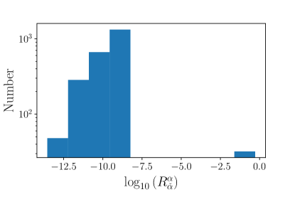
While we have mainly considered geometries in the Tree ensemble, we will also briefly discuss the F-theory base geometry which is believed to support the largest number of flux vacua (), denoted by Taylor and Wang (2015). This geometry has a non-Higgsable gauge sector of the form , and has 98 axions. We again consider gauge-oriented reheatons, and compute . The distribution is shown in Fig. 7. Clearly this distribution is consistent with the asymmetric couplings that we saw in the Tree ensemble: the ratios tend to be small. However, from Fig. 7 we see that actually gives rise to couplings that are even more asymmetric than in the Tree ensemble: there are no instances of , and the right tail of entries with is quite small compared to the bulk. In fact, there are 32 entries in the right tail, which readily yields a simple geometric explanation: the only pairs of gauge groups whose corresponding divisors intersect are the factors of . As there are 16 such factors, there are 32 gauge-oriented reheaton choices whose corresponding divisors intersect a divisor supporting another gauge group. This provides further evidence for our local geometric interpretation.
In conclusion, asymmetric reheating is even easier to arrange in , compared to the Tree ensemble. Via this mechanism, if the reheaton is oriented along an or gauge sector, it will only significantly reheat that sector. If the reheaton is oriented along a or , then it will reheat that sector as well as an additional or , respectively.
III.7 Saxion reheatons
As a final note in this section we will briefly comment on how our analysis applies to saxion reheatons. From Lagrangian Eq. II, we see that the couplings of a given saxion to the gauge fields is actually the same as its axion partner, with . In the context of string compactifications, since the Kähler metric for Kähler moduli applies to both their saxion and axion components, our analysis thus far applies equally well to the saxion-gauge field couplings. However, since the saxions are not protected by a discrete shift symmetry, we expect the potential of the saxions to be richer than that of the axions after supersymmetry breaking, which could include extra couplings that lead to higher decay rates than the dimension five coupling to gauge fields that we study. Whether asymmetric reheating persists in this regime for saxions requires a careful analysis, but in the absence of these additional couplings our result also holds for saxions.
IV Reheated Gauge Groups
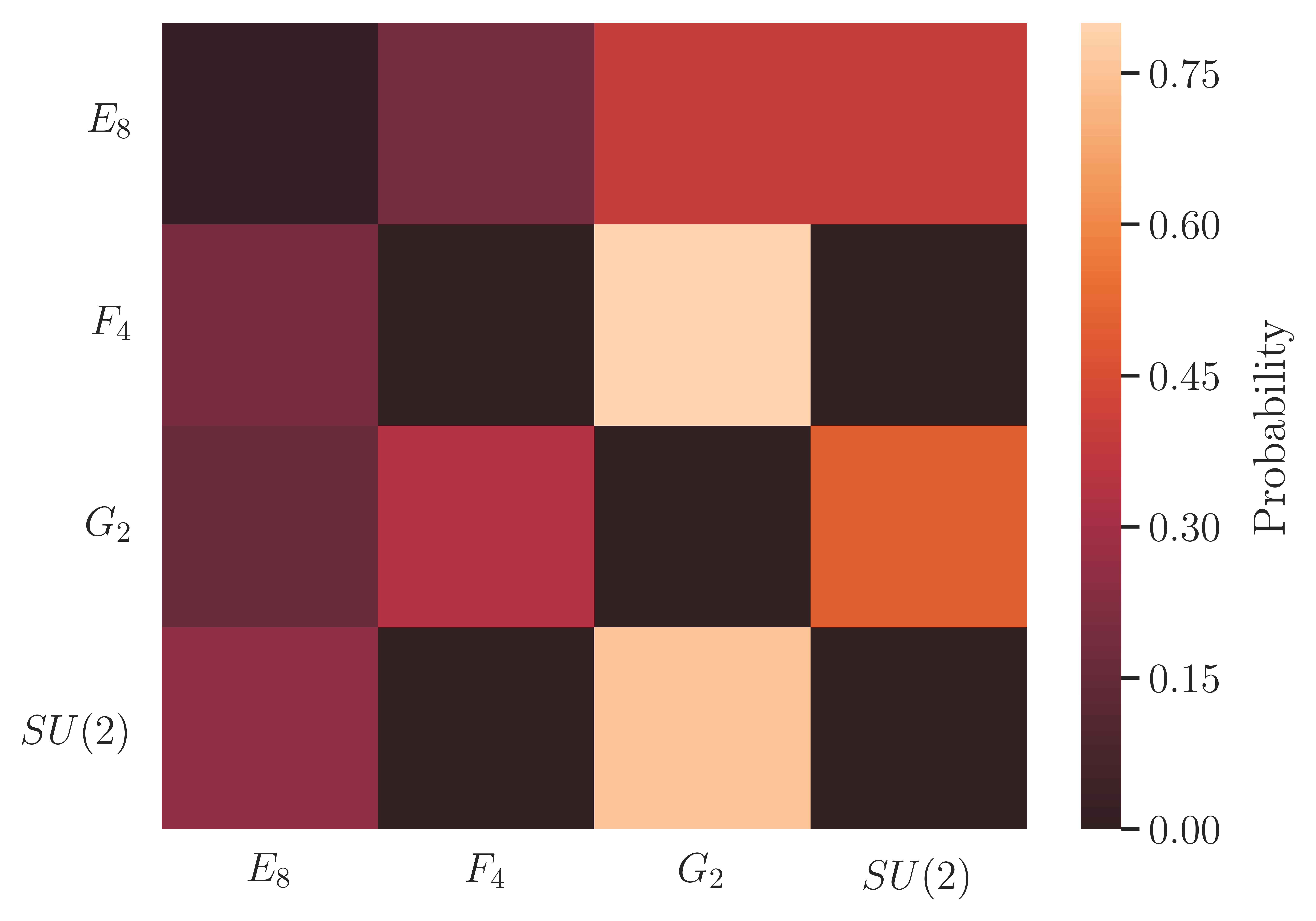
Thus far, we have demonstrated asymmetric couplings of axions, determined by both topological structure and the position in Kähler moduli space. It is natural to ask, what does this imply about correlations between various gauge sectors? In Fig. 8 we show the probability distribution of a -oriented reheaton to couple significantly ( ) to a gauge sector . The distribution is quite interesting. The axion-reheatons oriented along gauge groups apart from and also tend to significantly couple to an universally. However, axion-reheatons oriented along or instead tend to significantly couple to another . As an example let us consider the reheatons oriented along , which exists (to high probability) on so-called height-4 rays (see Halverson et al. (2017b) for further details). The most significantly couplings are to and other gauge group, with a smaller fraction to .
From the topological point of view we can consider all of the tree configurations and their corresponding gauge groups, and ask which gauge groups are most likely to be connected to via divisor intersections. To do so we make a technical assumption, which is that the initial point over which the tree was placed was defined by a triple intersection of divisors carrying gauge groups (this assumption is of very high probability in the Tree ensemble Halverson et al. (2017b)). It is then the case that every single in the tree ensemble shares an edge with a : there is a universal that arises in the first blowup, and arises from a blowup along an edge connecting that to a vertex. If another is present, whether or not the intersects with the other is a question of the particular tree, and this occurs about of the time. The case of an coupling is similar, and a given intersects an at a frequency of about . This statistics roughly resemble the plot given in Fig. 8, though of course moduli-dependent data also enter the reheating coefficients, not just topological data. With this topological correlation in mind, one should note that the preference of an -oriented reheaton to couple significantly to other ’s should be taken with a grain of salt, as we have not included trees over edges in this analysis. Such trees will generically separate interesting divisor, and we therefore expect that this preference is an artifact of our analysis.
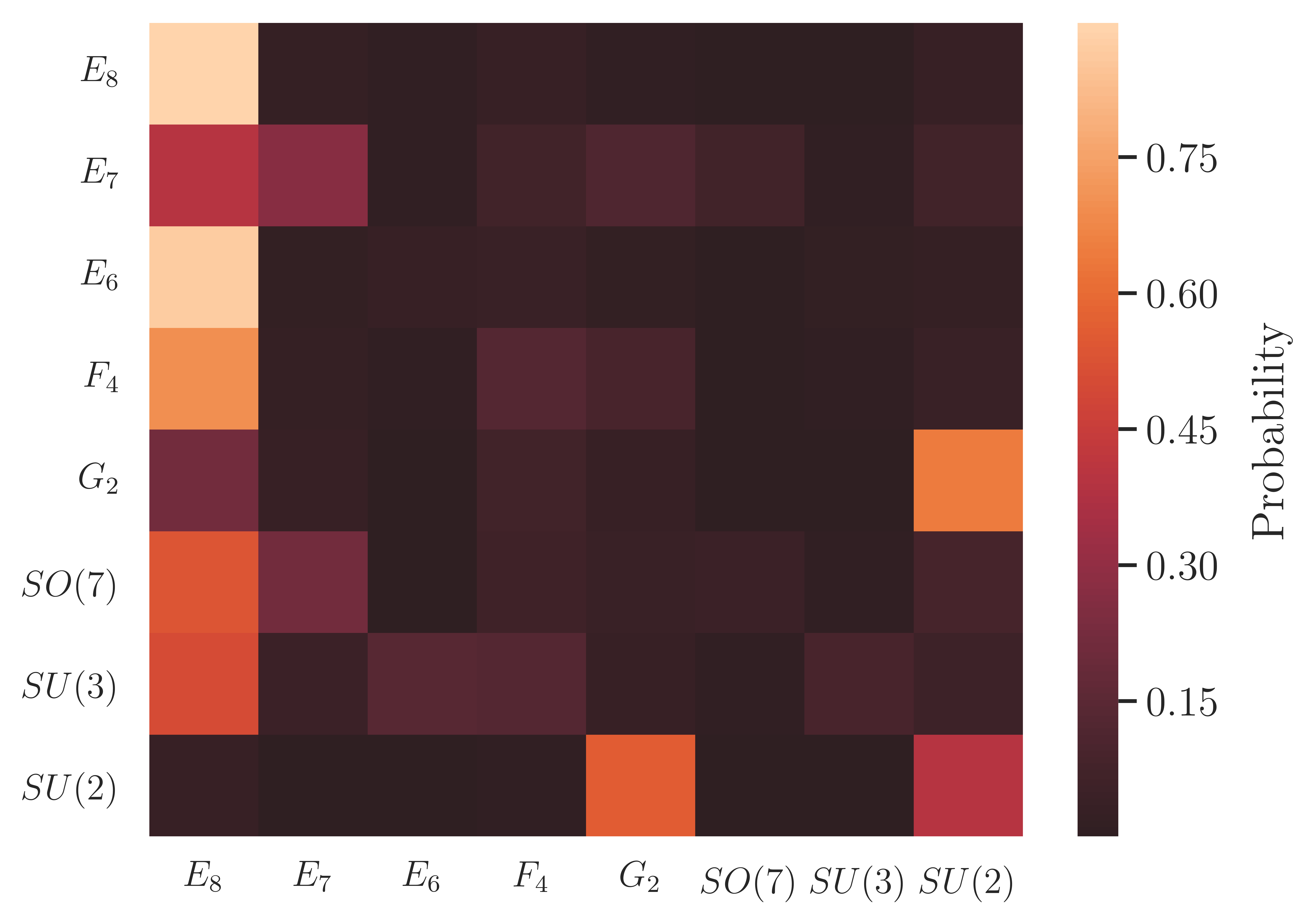
As a final consideration, we note that we have concentrated on trees over points, but one could also consider trees over curves as well. The structure is not nearly as rich, as there are only 82 allowed trees over curves in the Tree ensemble, but we expect this to alter the distribution shown in Fig. 8 somewhat. Above we gave evidence that the distribution for the -aligned reheaton roughly coincides with the distribution of topological intersections of gauge group divisor in the Tree ensemble. With that in mind, we will estimate the effect that trees over edges will have on our correlations by considering such intersections for trees over curves. We make the high probability assumption that the two divisors, whose intersection defines the curve over which the tree is placed, both carry an gauge group. Using this high-probability technical assumption the probability distribution is shown in Fig 9. This assumption restricts the type of gauge groups carried by the divisors in the tree to those that appear in Fig 9. From this distribution we anticipate the main effect of including curve tree is to shift the preference of an -oriented reheaton from another to , and to virtually eliminate the preference of an -oriented reheaton to couple to another .
V Discussion
In this work we demonstrated that asymmetric axion reheating arises in F-theory compactifications that have large numbers of axions and gauge sectors. We computed couplings relevant for reheating, in particular the couplings of axions to gauge groups in a large ensemble of F-theory geometries and also the F-theory geometry with the most flux vacua, both of which generically exhibit large numbers of axions and gauge sectors.
The distributions of coupling ratios are non-trivial. One main result is that gauge-oriented axions couple to of the total gauge sectors with couplings, while randomly drawn combinations of those axions couple to . In the gauge-oriented case, the peak of the distribution is far below zero. Asymmetric reheating occurs in both cases, and leads to reheating that is more asymmetric than in bottom-up models obtained from either Wilson coefficients or random EFTs.
Another result in the gauge-oriented axion case is that the leading couplings admit an interpretation that is local in the string geometry. Specifically, their ratios of reheating couplings depend critically on local intersection structure. These ratios are a function of both discrete topological structure and continuous Kähler moduli.
Of course, this is only a first step in understanding reheating dynamics in broad classes of string compactifications. For instance, we have not included additional couplings of the axions to the saxions (and other moduli), such as those that would be generated by a non-perturbative superpotential. Such couplings could in principle be dangerous for asymmetric reheating, as one could imagine a scenario in which saxions become excited and themselves contribute to reheating.555We thank Liam McAllister for discussion on this point.
In addition, we have not yet identified candidate reheatons in this setup, but have instead taken an agnostic approach. One option is that the reheaton is not connected to inflation, but is instead simply a scalar field that comes to dominate the energy density of the universe and decays prior to nucleosynthesis; this is relatively simple, but depends on moduli stabilization and supersymmetry breaking. Another possibility is that reheaton is the inflaton, which requires identifying which axion direction begins to oscillate at the end of inflation. This hard problem requires control over inflationary trajectories in high-dimensional scalar potentials. Both cases require control over the scalar potential and need to be computed with care.
Finally, we return to one of our motivations: reheating too many degrees of freedom in string compactifications can lead to severe cosmological problems that disagree with observations, such as the overproduction of dark matter. Though avoiding these problems is model-dependent, our result that asymmetric reheating arises naturally in large string ensembles could play a major role in obtaining realistic post-inflationary cosmologies.
Acknowledgements. We thank JiJi Fan, Liam McAllister, Fernando Quevedo, Fabian Ruehle, Jessie Shelton, and Scott Watson for useful discussion. We acknowledge generous support provided by the Northeastern University Discovery Cluster. J.H. is supported by NSF grant PHY-1620526. B.N. is supported by NSF grant PHY-PHY-1620575.
References
- Guth (1981) A. H. Guth, Phys. Rev. D 23, 347 (1981).
- Linde (1982) A. D. Linde, QUANTUM COSMOLOGY, Phys. Lett. 108B, 389 (1982), [Adv. Ser. Astrophys. Cosmol.3,149(1987)].
- Abbott et al. (1982) L. Abbott, E. Farhi, and M. B. Wise, Physics Letters B 117, 29 (1982).
- Dolgov and Linde (1982) A. D. Dolgov and A. D. Linde, Phys. Lett. 116B, 329 (1982).
- Albrecht et al. (1982) A. Albrecht, P. J. Steinhardt, M. S. Turner, and F. Wilczek, Phys. Rev. Lett. 48, 1437 (1982).
- Kofman et al. (1994) L. Kofman, A. D. Linde, and A. A. Starobinsky, Phys. Rev. Lett. 73, 3195 (1994), arXiv:hep-th/9405187 [hep-th] .
- Shtanov et al. (1995) Y. Shtanov, J. H. Traschen, and R. H. Brandenberger, Phys. Rev. D51, 5438 (1995), arXiv:hep-ph/9407247 [hep-ph] .
- Traschen and Brandenberger (1990) J. H. Traschen and R. H. Brandenberger, Phys. Rev. D42, 2491 (1990).
- Adshead et al. (2015) P. Adshead, J. T. Giblin, T. R. Scully, and E. I. Sfakianakis, JCAP 1512, 034 (2015), arXiv:1502.06506 [astro-ph.CO] .
- Garcia-Bellido and Linde (1998) J. Garcia-Bellido and A. D. Linde, Phys. Rev. D57, 6075 (1998), arXiv:hep-ph/9711360 [hep-ph] .
- Cuissa and Figueroa (2018) J. R. C. Cuissa and D. G. Figueroa, (2018), arXiv:1812.03132 [astro-ph.CO] .
- Halverson et al. (2017a) J. Halverson, B. D. Nelson, and F. Ruehle, Phys. Rev. D95, 043527 (2017a), arXiv:1609.02151 [hep-ph] .
- Halverson et al. (2018a) J. Halverson, B. D. Nelson, F. Ruehle, and G. Salinas, Phys. Rev. D98, 043502 (2018a), arXiv:1805.06011 [hep-ph] .
- Kolb et al. (1985) E. W. Kolb, D. Seckel, and M. S. Turner, Nature 314, 415 (1985).
- Berezhiani et al. (1996) Z. G. Berezhiani, A. D. Dolgov, and R. N. Mohapatra, Phys. Lett. B375, 26 (1996), arXiv:hep-ph/9511221 [hep-ph] .
- Adshead et al. (2016) P. Adshead, Y. Cui, and J. Shelton, JHEP 06, 016 (2016), arXiv:1604.02458 [hep-ph] .
- Gross et al. (1985) D. J. Gross, J. A. Harvey, E. J. Martinec, and R. Rohm, In *Argonne/Chicago 1985, Proceedings, Anomalies, Geometry, Topology*, 299-313 and Preprint - GROSS, D.J. (84,REC.JAN.85) 11p, Phys. Rev. Lett. 54, 502 (1985).
- Lerche et al. (1987) W. Lerche, D. Lust, and A. N. Schellekens, Nucl. Phys. B287, 477 (1987), [,477(1986)].
- Vafa (1996) C. Vafa, Nucl. Phys. B469, 403 (1996), arXiv:hep-th/9602022 [hep-th] .
- Morrison and Vafa (1996) D. R. Morrison and C. Vafa, Nucl. Phys. B476, 437 (1996), arXiv:hep-th/9603161 [hep-th] .
- Taylor and Wang (2015) W. Taylor and Y.-N. Wang, JHEP 12, 164 (2015), arXiv:1511.03209 [hep-th] .
- Halverson et al. (2017b) J. Halverson, C. Long, and B. Sung, Phys. Rev. D96, 126006 (2017b), arXiv:1706.02299 [hep-th] .
- Taylor and Wang (2018) W. Taylor and Y.-N. Wang, JHEP 01, 111 (2018), arXiv:1710.11235 [hep-th] .
- Kofman and Yi (2005) L. Kofman and P. Yi, Phys. Rev. D72, 106001 (2005), arXiv:hep-th/0507257 [hep-th] .
- Cicoli and Mazumdar (2010) M. Cicoli and A. Mazumdar, JCAP 1009, 025 (2010), arXiv:1005.5076 [hep-th] .
- Blumenhagen and Plauschinn (2014) R. Blumenhagen and E. Plauschinn, Phys. Lett. B736, 482 (2014), arXiv:1404.3542 [hep-th] .
- Halverson (2017) J. Halverson, Nucl. Phys. B919, 267 (2017), arXiv:1603.01639 [hep-th] .
- Halverson et al. (2017c) J. Halverson, C. Long, and P. Nath, Phys. Rev. D96, 056025 (2017c), arXiv:1703.07779 [hep-ph] .
- Blumenhagen et al. (2009) R. Blumenhagen, M. Cvetic, S. Kachru, and T. Weigand, Ann. Rev. Nucl. Part. Sci. 59, 269 (2009), arXiv:0902.3251 [hep-th] .
- Carifio et al. (2018) J. Carifio, W. J. Cunningham, J. Halverson, D. Krioukov, C. Long, and B. D. Nelson, Phys. Rev. Lett. 121, 101602 (2018), arXiv:1711.06685 [hep-th] .
- Hayakawa (1995) Y. Hayakawa (1995).
- lung Wang (1997) C. lung Wang, “On the incompleteness of the weil-petersson metric along degenerations of calabi-yau manifolds,” (1997).
- Grassi (1991) A. Grassi, Mathematische Annalen 290, 287 (1991).
- Morrison and Taylor (2012a) D. R. Morrison and W. Taylor, Central Eur. J. Phys. 10, 1072 (2012a), arXiv:1201.1943 [hep-th] .
- Morrison and Taylor (2012b) D. R. Morrison and W. Taylor, Fortsch. Phys. 60, 1187 (2012b), arXiv:1204.0283 [hep-th] .
- Grassi et al. (2015) A. Grassi, J. Halverson, J. Shaneson, and W. Taylor, JHEP 01, 086 (2015), arXiv:1409.8295 [hep-th] .
- Morrison and Taylor (2015) D. R. Morrison and W. Taylor, JHEP 05, 080 (2015), arXiv:1412.6112 [hep-th] .
- Halverson and Taylor (2015) J. Halverson and W. Taylor, JHEP 09, 086 (2015), arXiv:1506.03204 [hep-th] .
- Taylor and Wang (2016) W. Taylor and Y.-N. Wang, JHEP 01, 137 (2016), arXiv:1510.04978 [hep-th] .
- Cvetic et al. (2019) M. Cvetic, J. Halverson, L. Lin, M. Liu, and J. Tian, (2019), arXiv:1903.00009 [hep-th] .
- Halverson et al. (2018b) J. Halverson, C. Long, and B. Sung, JHEP 02, 113 (2018b), arXiv:1710.09374 [hep-th] .
- Halverson and Langacker (2018) J. Halverson and P. Langacker, Proceedings, Theoretical Advanced Study Institute in Elementary Particle Physics: Physics at the Fundamental Frontier (TASI 2017): Boulder, CO, USA, June 5-30, 2017, PoS TASI2017, 019 (2018), arXiv:1801.03503 [hep-th] .
- Cicoli et al. (2008) M. Cicoli, J. P. Conlon, and F. Quevedo, JHEP 10, 105 (2008), arXiv:0805.1029 [hep-th] .
- Berg et al. (2005a) M. Berg, M. Haack, and B. Kors, Phys. Rev. D71, 026005 (2005a), arXiv:hep-th/0404087 [hep-th] .
- Berg et al. (2005b) M. Berg, M. Haack, and B. Kors, JHEP 11, 030 (2005b), arXiv:hep-th/0508043 [hep-th] .
- Demirtas et al. (2018) M. Demirtas, C. Long, L. McAllister, and M. Stillman, (2018), arXiv:1808.01282 [hep-th] .
- He (2017) Y.-H. He, (2017), arXiv:1706.02714 [hep-th] .
- Ruehle (2017) F. Ruehle, JHEP 08, 038 (2017), arXiv:1706.07024 [hep-th] .
- Carifio et al. (2017) J. Carifio, J. Halverson, D. Krioukov, and B. D. Nelson, JHEP 09, 157 (2017), arXiv:1707.00655 [hep-th] .