One-Pass Sparsified Gaussian Mixtures

Abstract

We present a one-pass sparsified Gaussian mixture model (SGMM). Given N data points in P dimensions X, the model fits K Gaussian distributions to X and (softly) classifies each point to these clusters. After paying an up-front cost of O(NP log P) to precondition the data, we subsample Q entries of each data point and discard the full P-dimensional data. SGMM operates in O(KNQ) time per iteration for diagonal or spherical covariances, independent of P, while estimating the model parameters in the full P-dimensional space, making it one-pass and hence suitable for streaming data. We derive the maximum likelihood estimators for the parameters in the sparsified regime, demonstrate clustering on synthetic and real data, and show that SGMM is faster than GMM while preserving accuracy.

I Introduction

When performing clustering analysis on high-dimensional ($P$ features), high-volume ($N$ samples) data, it is common to employ simple clustering schemes like $k$-means and $k$-nearest-neighbors, particularly during data exploration and feature engineering, because these techniques are fast and return informative results [1]. Often each data point $\mathbf{x}_{i}\in\mathbb{R}^{P}$ will be seen only once and must then be discarded, necessitating one-pass algorithms [2]. Further, the latent dimension $P$ may be prohibitively large or the rate of data acquisition may be too high to permit analysis on the full data.

We present a clustering algorithm suitable for this regime: the sparsified Gaussian mixture model (SGMM), building on our previous work in which we developed the sparsification scheme we use here and applied it to $k$-means clustering [3]. TheGaussian mixture model, in particular when using diagonal or spherical covariances, is a natural extension of $k$-means: it increases generalizability by taking into account cluster size and covariance and by performing soft clustering, while still being relatively inexpensive to compute [4].

SGMM works on compressed data, such that the computation and storage costs scale with $Q\ll P$ instead of $P$, and yet the algorithm is one-pass, meaning that the model parameters are estimated in the full $P$-dimensional space. These requirements are seemingly orthogonal to each other; we are able to provide both by a careful choice of how we compress the data, which we do using a sketch $\mathbf{R}_{i}^{T}\mathbf{x}_{i}$ of size $Q\ll P$. Our sketching scheme is motivated by the Johnson-Lindenstrauss lemma [5], which states that certain random projections into lower dimensions preserve pairwise distances to within a small error $\varepsilon$ with high probability. In particular, these embeddings can be computed efficiently in $\mathcal{O}(NP\log P)$ time [6], and the data are recoverable from the embeddings when they are sparse in some basis [7].

The idea is to project the data into a lower dimension and perform analyses there, where it is cheap to do so. A variety of approaches have been proposed to this end [8, 9, 10, 11, 12], including several applications of sketching to clustering algorithms [13, 3, 14, 11, 15, 12] and Gaussian mixtures specifically [16]. In general, such compressive approaches are two-pass, meaning that access to the full data is required to estimate statistics in the original space, such as the sample mean. The contribution of our method is that it is compressive and one-pass, meaning that we estimate statistics in the full $P$-dimensional space using only $Q$-dimensional sketches of the data. This is possible because we use a different sampling matrix $\mathbf{R}_{i}$ for each data point $\mathbf{x}_{i}$, so that the $Q$ features of some dense statistic ${\bm{\theta}}$ informed by $\mathbf{x}_{i}$ are in general not the same as the $Q$ features informed by another data point $\mathbf{x}_{j}$. Additionally, the the quantities we derive (such as mixture responsibilities and the Mahalanobis distance) may be useful building blocks for future algorithms using our sketching scheme.

The paper is organized as follows. In Section II we discuss the theoretical foundations and prove our main results. Then, in Section III we present the sparsified Gaussian mixture model algorithm and discuss its implementation and complexity. In Section IV we show simulation results, and we summarize and conclude in Section V.

II Theory

II-A Data Sketching

A sketch of a matrix $\mathbf{X}=[\mathbf{x}_{1},\mathbf{x}_{2},\ldots,\mathbf{x}_{N}]^{T}\in\mathbb{R}^{N\times P}$ is a random low-dimensional projection of $\mathbf{X}$ [17]. Sketching is typically used to obtain a low-rank approximation ${\mathbf{X}}_{Q}$ with rank $Q\ll P$ such that $\left\lVert{\mathbf{X}}_{Q}-\mathbf{X}\right\rVert_{F}$ is minimal. There are alternative ways to find such an $\mathbf{X}_{Q}$, e.g. principal components analysis or feature selection, but sketching provides several advantages [18]. Sketching via random projections is oblivious, meaning that the sketching operator can be constructed without seeing the data $\mathbf{X}$. This makes sketching particularly well-suited to streaming and distributed applications [19, 3, 20]. Cost-preserving sketches reduce the dimension of $\mathbf{X}$ in such a way that certain cost functions (for example, Euclidean distance in the case of $k$-means clustering) are preserved within a low tolerance $\varepsilon$ with high probability [12]. More generally, sketches are often optimal in the sense that they achieve the lower bound on some error [21, 22, 20, 23, 18]. Finally, sketches are fast to compute, typically $\mathcal{O}(NP\log P)$ for $N$ data points in $P$ dimensions [17, 6].

There is a broad literature on sketching, establishing state-of-the-art bounds on the compressed dimension $Q$ in terms of the number of data points $N$, the acceptable error $\varepsilon$, and the original dimension $P$, and optimizing tradeoffs between error bounds, time, and space complexity [12, 18, 6]. There are a variety of ways to carry out the sketch in practice, including the original approach using dense iteratively constructed Gaussian matrices, trinary matrices with sparsity $2/3$ [8], and several constructions sparser still [24]. Here we use a method inspired by the Fast Johnson-Lindenstrauss Transform [6] and described in detail in our previous work [3].

We will project $\mathbf{x}_{i}$ into a lower dimension by keeping $Q\ll P$ components chosen uniformly at random. Before doing so we precondition the data using a random orthonormal system (ROS):

$$\mathbf{x}_{i}=\mathbf{H}\mathbf{D}\mathbf{x}_{i}^{raw}$$ (1)

where $\mathbf{D}$ is diagonal with entries $\pm 1$ chosen uniformly at random and $\mathbf{H}$ is a discrete cosine transform matrix. The ROS transformation ensures that, with high probability, the magnitudes of the entries of $\mathbf{x}_{i}$ are relatively close to each other [25, 6], minimizing the risk of “missing” the information in the vector when subsampling. The preconditioning operator $\mathbf{H}\mathbf{D}$ is the same for all $\mathbf{x}_{i}$, and can be applied and inverted in $\mathcal{O}(NP\log P)$ time to the full dataset $\{\mathbf{x}_{1},\mathbf{x}_{2},\ldots,\mathbf{x}_{N}\}$, which is the dominant cost in our algorithm for small enough sketches. A detailed discussion of convergence properties and bounds of the ROS can be found in [3]. Henceforth, when we write $\mathbf{x}_{i}$ we assume the data have been preconditioned.

Following the preconditioning, we subsample $Q\ll P$ entries chosen uniformly at random from $\mathbf{x}_{i}$. This operation can be represented by the product $\mathbf{R}_{i}^{T}\mathbf{x}_{i}$ where $\mathbf{R}_{i}\in\mathbb{R}^{P\times Q}$ is sparse, with $\mathbf{R}_{i}(p,q)=1$ if we are keeping the $p$th feature of $\mathbf{x}_{i}$ and storing it in the $q$th dimension of the sparsified vector, and 0 otherwise. Thus $\mathbf{R}_{i}^{T}\mathbf{x}_{i}\in\mathbb{R}^{Q}$ are the entries we preserve from $\mathbf{x}_{i}$. In practice we store only the $Q$ entries of $\mathbf{x}_{i}$ that the subsampling picks out as well as the indices specifying which entries were preserved (the indices of the $Q$ non-zero rows of $\mathbf{R}_{i}$), though it will facilitate our exposition to write quantities like $\mathbf{R}_{i}\mathbf{R}_{i}^{T}\mathbf{x}_{i}\in\mathbb{R}^{P}$. Crucially, $\mathbf{R}_{i}$ is resampled for each $\mathbf{x}_{i}$. This fact is what enables the method to be one-pass.

II-B Mixture Models

We now describe the modeling framework, beginning with a general mixture model [4]. Assume there are $K$ components and that each data point $\mathbf{x}_{i}$ belongs to one of them, indicated by the hidden variable $z_{i}\in\{1,2,\ldots K\}$. A mixture model [4] is fully specified by the component distributions $p_{k}(\mathbf{x}_{i}\mid{\bm{\theta}}_{k})=p(\mathbf{x}_{i}\mid z_{i}=k,{\bm{\theta}}_{k})$, the component weights $\bm{\pi}=\{\pi_{k}\}_{k=1}^{K}$ with $\sum\pi_{k}=1$, and the parameters ${\bm{\theta}}=\{{\bm{\theta}}_{k}\}_{k=1}^{K}$. The distribution for $x_{i}$ is given by

$$p(\mathbf{x}_{i}\mid{\bm{\theta}}_{k})=\sum_{k=1}^{K}\pi_{k}p_{k}(\mathbf{x}_{i}\mid{\bm{\theta}}_{k}).$$ (2)

For a mixture of Gaussians, ${\bm{\theta}}_{k}=\{\bm{\mu}_{k},\mathbf{S}_{k}\}$ where $\bm{\mu}_{k}\in\mathbb{R}^{P}$ is the mean and $\mathbf{S}_{k}\in\mathbb{R}^{P\times P}$ is the covariance of the $k$th cluster, and $p(\mathbf{x}_{i}\mid z_{i}=k,{\bm{\theta}}_{k})$ is given by

$$p_{k}(\mathbf{x}_{i}\mid{\bm{\theta}}_{k})=\frac{1}{(2\pi)^{P/2}}\frac{1}{|\mathbf{S}_{k}|^{1/2}}\exp\left(-\frac{1}{2}D_{{\bm{\theta}}_{k}}(\mathbf{x}_{i})\right)$$ (3)

where

$$D_{{\bm{\theta}}_{k}}(\mathbf{x}_{i})=\big{(}\mathbf{x}_{i}-\bm{\mu}_{k}\big{)}^{T}\bm{\Lambda}_{k}\big{(}\mathbf{x}_{i}-\bm{\mu}_{k}\big{)}$$ (4)

is the squared Mahalanobis distance and $\bm{\Lambda}_{k}=\mathbf{S}_{k}^{-1}$ is the $k$th precision matrix.

The goal is to simultaneously estimate the parameters ${\bm{\theta}}$, the weights $\bm{\pi}$, and the cluster assignments $z_{i}$, which we do using the Expectation-Maximization algorithm.

II-C The EM Algorithm

The log likelihood for data $\mathcal{X}=\{\mathbf{x}_{1},\mathbf{x}_{2},\ldots\mathbf{x}_{N}\}$ under the mixture distribution given in equation (2) is

$$\ell(\bm{\theta})=\sum_{i=1}^{N}\log\left(\sum_{k=1}^{K}p_{k}(\mathbf{x}_{i}\mid{\bm{\theta}}_{k})\right).$$ (5)

In the case of GMM’s (as well as in many others) it is intractable to find the maximum likelihood estimators (MLE’s) for $\bm{\theta}$ because of the hidden $\mathbf{z}=\{z_{i}\}_{i=1}^{N}$. Expectation-Maximization finds a local optimum by iteratively holding one of the unknown quantities (${\bm{\theta}}$ or $\mathbf{z}$) fixed and solving for the other. At each iteration we obtain a new estimate $\{{\bm{\theta}}^{t},\bm{\pi}^{t}\}$ computed from the previous estimate $\{{\bm{\theta}}^{t-1},\bm{\pi}^{t-1}\}$. Specifically, define the auxiliary function

$$Q({\bm{\theta}},{\bm{\theta}}^{t-1})=E\left[\ell_{c}({\bm{\theta}})\mid\mathcal{X},{\bm{\theta}}^{t-1}\right]$$ (6)

where

$$\ell_{c}({\bm{\theta}})=\sum_{i,k}\log p\left(\mathbf{x}_{i},z_{i}=k\mid{\bm{\theta}}_{k}\right)$$ (7)

is the complete data log likelihood and $\mathcal{X}$ is the dataset.

The E step is then to compute the expected sufficient statistics in $Q$ for ${\bm{\theta}}$, which is equivalent to finding the responsibility $r_{ik}=p(z_{i}=k\mid\mathbf{x}_{i},{\bm{\theta}}^{t-1})$ for each data point $\mathbf{x}_{i}$ and component $k$:

$$r_{ik}=\frac{\pi_{k}p_{k}(\mathbf{x}_{i}\mid{\bm{\theta}}_{k}^{t-1})}{\sum_{j=1}^{K}\pi_{j}p_{j}\big{(}\mathbf{x}_{i}\mid{\bm{\theta}}_{j}^{t-1}\big{)}}.$$ (8)

The auxiliary function in equation (6) can then be expressed in terms of the responsibility as

$$Q({\bm{\theta}},{\bm{\theta}}^{t-1})=\sum_{i,k}r_{ik}\log\left[\pi_{k}p_{k}(\mathbf{x}_{i}\mid{\bm{\theta}}_{k})\right].$$ (9)

Figure 1: Error in $p_{k}^{\mathcal{R}}$ as a function of compression. 10000 $\mathbf{x}_{i}\sim\mathcal{N}(0,1)$ in 100 dimensions per trial. Inset: error in ${D_{{\bm{\theta}}_{k}}^{\mathcal{R}}(\mathbf{x}_{i})}$.

The M step is to obtain the next iterate $\{{\bm{\theta}}^{t},\bm{\pi}^{t}\}$ by optimizing $Q$:

$$\{\bm{\theta}^{t},\bm{\pi}^{t}\}=\text{argmax}_{{\bm{\theta}},\bm{\pi}}Q({\bm{\theta}},{\bm{\theta}}^{t-1}).$$ (10)

For a mixture of Gaussians, $Q$ is optimized by the the maximum likelihood estimators:

$$\widehat{\pi}_{k} = \frac{r_{k}}{N}$$ (11)

$$\widehat{\bm{\mu}}_{k} = \frac{\sum_{i}r_{ik}\mathbf{x}_{i}}{\sum_{i}r_{ik}}$$ (12)

$$\widehat{\mathbf{S}}_{k} = \frac{\sum_{i}r_{ik}(\mathbf{x}_{i}-\widehat{\bm{\mu}}_{k})(\mathbf{x}_{i}-\widehat{\bm{\mu}}_{k})^{T}}{\sum_{i}r_{ik}}$$ (13)

The E and M steps are repeated until (guaranteed) convergence to a local maximum or saddle point of $Q$.

II-D EM for Sparsified Gaussian Mixtures

We now present our main result, the EM algorithm for sparsified Gaussian mixtures; i.e., the equivalents to the responsibility in equation (8) and the parameter MLE’s in equations (11-13) under sparsification.

The sparsified analog of the squared Mahalanobis distance in equation (4) is

$${D_{{\bm{\theta}}_{k}}^{\mathcal{R}}(\mathbf{x}_{i})}=\big{(}\mathbf{x}_{i}-\bm{\mu}_{k}\big{)}^{T}{\bm{\Lambda}^{\mathcal{R}_{i}}_{k}}\big{(}\mathbf{x}_{i}-\bm{\mu}_{k}\big{)}$$ (14)

where

$${\bm{\Lambda}^{\mathcal{R}_{i}}_{k}}={\mathbf{R}_{i}}({\mathbf{R}_{i}}^{T}\mathbf{S}_{k}{\mathbf{R}_{i}})^{-1}{\mathbf{R}_{i}}^{T}\in\mathbb{R}^{P\times P}$$ (15)

is the sparsified analog of the precision matrix $\bm{\Lambda}_{k}=\mathbf{S}_{k}^{-1}$. The sparsified Gaussian density is:

$$p_{k}^{\mathcal{R}}(\mathbf{x}_{i}\mid{\bm{\theta}}_{k})=\frac{1}{{2\pi}^{Q/2}}\frac{1}{|{\mathbf{R}_{i}}^{T}\mathbf{S}_{k}{\mathbf{R}_{i}}|^{1/2}}\exp\left(-\frac{1}{2}D^{\mathcal{R}}_{{\bm{\theta}}_{k}}(\mathbf{x}_{i})\right).$$ (16)

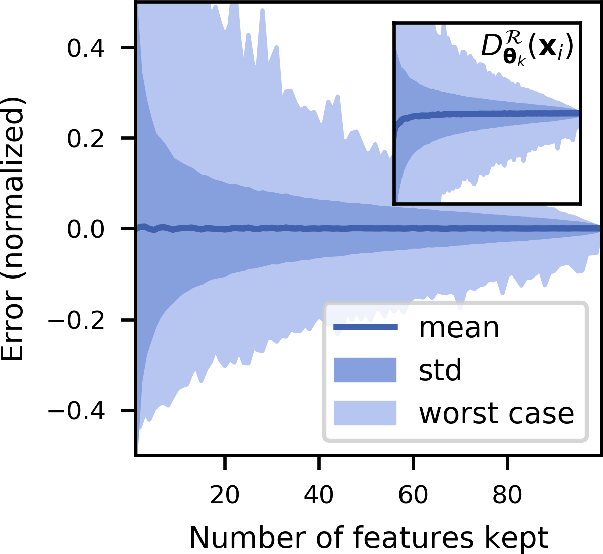
This can be taken to be a $Q$-dimensional Gaussian with mean ${\mathbf{R}_{i}}\bm{\mu}_{k}$ and covariance ${\mathbf{R}_{i}}^{T}\mathbf{S}_{k}{\mathbf{R}_{i}}$ evaluated at ${\mathbf{R}_{i}}\mathbf{x}_{i}$. Both $p^{\mathcal{R}}$ and ${D_{{\bm{\theta}}_{k}}^{\mathcal{R}}(\mathbf{x}_{i})}$ are unbiased estimators of their dense counterparts when scaled by $P/Q$ (see Figure 1).

The E-step is to compute the responsibility as given in equation (8). Under sparsification, the responsbility becomes

$${r^{\mathcal{R}}_{i{k}}}=\frac{\pi_{k}p_{k}^{\mathcal{R}}(\mathbf{x}_{i}\mid{\bm{\theta}}_{k}^{t-1})}{\sum_{j=1}^{K}\pi_{j}p^{\mathcal{R}}_{j}\big{(}\mathbf{x}_{i}\mid{\bm{\theta}}_{k}^{t-1}\big{)}}$$ (17)

and hence the sparsified auxiliary function $Q$ in equation (9) is:

$$Q^{\mathcal{R}}({\bm{\theta}},{\bm{\theta}}^{t-1})=\sum_{i,k}{r^{\mathcal{R}}_{i{k}}}\log\left[\pi_{k}p_{k}^{\mathcal{R}}(\mathbf{x}_{i}\mid{\bm{\theta}}_{k})\right].$$ (18)

We now derive the maximum likelihood estimators for $\pi_{k}$ and ${\bm{\theta}}_{k}$ under sparsification.

Theorem 1 (Maximum Likelihood Estimators for Sparsified Gaussian Mixtures).

The maximum likelihood estimator for $\pi_{k}$ with respect to $Q^{\mathcal{R}}$ is

$$\widehat{{\pi}}_{k}^{\mathcal{R}}=\frac{\sum_{i}{r^{\mathcal{R}}_{i{k}}}}{N}.$$ (19)

The maximum likelihood estimators for $\bm{\mu}_{k}$ and $\mathbf{S}_{k}$ are the solutions to the system

$${\bm{\mu}}^{\mathcal{R}}_{k} = \left(\sum_{i}{r^{\mathcal{R}}_{i{k}}}{\bm{\Lambda}^{\mathcal{R}_{i}}_{k}}\right)^{\dagger}\sum_{i}{r^{\mathcal{R}}_{i{k}}}{\bm{\Lambda}^{\mathcal{R}_{i}}_{k}}\mathbf{x}_{i}$$ (20)

$$\sum_{i}{r^{\mathcal{R}}_{i{k}}}{\bm{\Lambda}^{\mathcal{R}_{i}}_{k}} = \sum_{i}{r^{\mathcal{R}}_{i{k}}}{\bm{\Lambda}^{\mathcal{R}_{i}}_{k}}\mathbf{M}_{ik}{\bm{\Lambda}^{\mathcal{R}_{i}}_{k}}$$ (21)

where

$$\mathbf{M}_{ik}=\big{(}\mathbf{x}_{i}-\bm{\mu}_{k}\big{)}\big{(}\mathbf{x}_{i}-\bm{\mu}_{k}\big{)}^{T}.$$ (22)

is the scatter matrix.

Proof.

The component of $Q^{\mathcal{R}}$ with $\pi_{k}$-dependence is

$$\ell^{\mathcal{R}}(\pi_{k})=\sum_{i,k}{r^{\mathcal{R}}_{i{k}}}\log\pi_{k}$$

from which the MLE in equation (19) can be derived by setting $\partial\ell^{\mathcal{R}}/\partial\pi_{k}=0$ for each $k$ simultanously and solving the resulting system. The components of $Q^{\mathcal{R}}$ with $\bm{\mu}_{k}$ and $\mathbf{S}_{k}$ dependence are

$$\ell^{\mathcal{R}}(\bm{\mu}_{k},\mathbf{S}_{k})=\sum_{i}{r^{\mathcal{R}}_{i{k}}}\left(\log|{\mathbf{R}_{i}}^{T}\mathbf{S}_{k}{\mathbf{R}_{i}}|+{D_{{\bm{\theta}}_{k}}^{\mathcal{R}}(\mathbf{x}_{i})}\right).$$ (23)

To find $\partial\ell^{\mathcal{R}}/\partial\bm{\mu}_{k}$ we observe that

$$\frac{\partial}{\partial\bm{\mu}_{k}}{D_{{\bm{\theta}}_{k}}^{\mathcal{R}}(\mathbf{x}_{i})}=-2{\bm{\Lambda}^{\mathcal{R}_{i}}_{k}}\big{(}\mathbf{x}_{i}-\bm{\mu}_{k}\big{)}.$$

Equation (20) then follows by setting $\partial\ell^{\mathcal{R}}/\partial\bm{\mu}_{k}=0$ and rearranging.

We now find $\partial\ell^{\mathcal{R}}/\partial\mathbf{S}_{k}$. For the first term in the summand of equation (23), we have that

$$\frac{\partial}{\partial\mathbf{S}_{k}}\log|{\mathbf{R}_{i}}^{T}\mathbf{S}_{k}{\mathbf{R}_{i}}|={\bm{\Lambda}^{\mathcal{R}_{i}}_{k}}$$ (24)

which can be obtained element-wise using Jacobi’s formula and the symmetry of $\mathbf{S}_{k}$. For the second term, we apply the “trace trick”:

$$D_{{\bm{\theta}}_{k}}^{\mathcal{R}}(\mathbf{x}_{i})=\text{tr}\left[\mathbf{M}_{ik}{\bm{\Lambda}^{\mathcal{R}_{i}}_{k}}\right]$$ (25)

to find

$$\frac{\partial}{\partial\mathbf{S}_{k}}D_{{\bm{\theta}}_{k}}^{\mathcal{R}}(\mathbf{x}_{i})=-{\bm{\Lambda}^{\mathcal{R}_{i}}_{k}}\mathbf{M}_{ik}{\bm{\Lambda}^{\mathcal{R}_{i}}_{k}},$$ (26)

which can be obtained by direct element-wise differentiation of equation (25). Setting $\partial\ell/\partial\mathbf{S}_{k}=0$ from equation (23) using equations (24) and (26) we obtain equation (21). ∎

Figure 2: Accuracy and timing of diagonal SGMM on the subset {0,3,9} of MNIST ($N=18003$) as a function of compression. Three initializations per trial, 20 trials per compression. Shaded regions indicate standard deviation (dark) and extrema (light) taken over the trials.

Evaluating these MLEs does not require access to the full $\mathbf{x}_{i}$, as in each case such terms are sparsified by the action of ${\bm{\Lambda}^{\mathcal{R}_{i}}_{k}}$. In the case of no sparsification; i.e., ${\mathbf{R}_{i}}=\mathbf{I}$ for all $i$, we recover the standard MLEs in equations (11 - 13). Equation (19) has only $\pi_{k}^{\mathcal{R}}$ dependence, and hence gives the MLE for this parameter. Equation (20) gives the MLE for $\bm{\mu}_{k}^{\mathcal{R}}$ in terms of the ${\bm{\Lambda}^{\mathcal{R}_{i}}_{k}}$. In the standard case, the $\bm{\Lambda}_{k}$ terms cancel and we obtain the MLE for $\bm{\mu}_{k}$, which is then used in place of $\bm{\mu}_{k}$ to find the MLE for $\mathbf{S}_{k}$; however, in the sparsified case we do not observe this cancelation, and hence must solve equations (20) and (21) simultaneously. This can be done, for example, in an EM-type iterative fashion, but such a procedure further requires the evaluation of ${\bm{\Lambda}^{\mathcal{R}_{i}}_{k}}$, involving a $Q\times Q$ inverse, of which there are $KN$ per iteration. These issues can be circumvented by using diagonal or spherical covariances. We give the MLEs for the diagonal case, $\mathbf{S}_{k}=\text{diag}(\mathbf{s}_{k})$ where $\mathbf{s}_{k}\in\mathbb{R}^{P}$ (proof omitted).

Corollary 2 (MLEs for diagonal $\mathbf{S}_{k}$).

When the $\mathbf{S}_{k}$ are diagonal, the system of equations (20 - 21) yields the MLEs

$$\widehat{\bm{\mu}}_{k} = \left(\sum_{i}{r^{\mathcal{R}}_{i{k}}}\mathbf{P}_{i}\right)^{\dagger}\sum_{i}{r^{\mathcal{R}}_{i{k}}}\mathbf{P}_{i}\mathbf{x}_{i}$$ (27)

$$\widehat{\mathbf{S}}_{k} = \text{diag}\left[\left(\sum_{i}{r^{\mathcal{R}}_{i{k}}}\mathbf{P}_{i}\right)^{\dagger}\sum_{i}{r^{\mathcal{R}}_{i{k}}}\mathbf{P}_{i}\mathbf{M}_{ik}\mathbf{P}_{i}\right]$$ (28)

where $\mathbf{P}_{i}\in\mathbb{R}^{P\times P}$ is the sparse projection matrix:

$$\mathbf{P}_{i}=\mathbf{R}_{i}\mathbf{R}_{i}^{T}.$$ (29)

In the case of diagonal covariances (as well as in the simpler spherical case in which $\mathbf{S}_{k}=s_{k}I$), the responsibilities ${r^{\mathcal{R}}_{i{k}}}$ (E step) and the updates for $\widehat{\bm{\mu}}_{k}$ and $\widehat{\mathbf{S}}_{k}$ (M step) can each be computed in $\mathcal{O}(KNQ)$ time. Thus the EM algoritm has time complexity $\mathcal{O}(KNQ)$ per iteration, in contrast to the standard diagonal GMM’s complexity of $\mathcal{O}(KNP)$ per iteration.

III Algorithm and Implementation

We now discuss the practical implementation of the SGMM algorithm. Thus far we have used notation expedient for mathematical exposition but not representative of how we perform computations in practice. For example, we do not perform the matrix multiplications in quantities $\mathbf{R}_{i}\mathbf{H}\mathbf{D}\mathbf{x}_{i}$, nor do we form most of the intermediate quantities in our calculations.

Algorithm 1 Preconditioned Random Projection

1:Given: Data $\{\mathbf{x}_{1},\mathbf{x}_{2},\ldots,\mathbf{x}_{N}\}$ with $\mathbf{x}_{i}\in\mathbb{R}^{P}$, sketch size $Q\ll P$

2:Generate preconditioning operator $\mathbf{H}\mathbf{D}$;

3:for $i=1\to N$ do

4:     Generate projection $\mathbf{R}_{i}^{T}$;

5:     Precondition and project $\mathbf{y}_{i}\leftarrow\mathbf{R}_{i}^{T}\mathbf{H}\mathbf{D}\mathbf{x}_{i}$;

6:     Discard $\mathbf{x}_{i}$;

7:Return $\{\mathbf{y}_{1},\ldots,\mathbf{y}_{N}\},\{\mathbf{R}_{i},\ldots,\mathbf{R}_{N}\},\mathbf{H},\mathbf{D}$;

Algorithm 1 shows the preconditioning and projection as a stand-alone algorithm. We need to generate and apply the preconditioning and subsampling operation $\mathbf{R}_{i}^{T}\mathbf{H}\mathbf{D}$ to each data point. Recall that $\mathbf{D}\in\mathbb{R}^{P\times P}$ is diagonal with entries $\pm 1$ chosen uniformly at random; it therefore suffices to store just the $\mathcal{O}(P)$ indices corresponding to the $-1$ entries, and computing $\mathbf{D}\mathbf{x}_{i}$ is a matter of flipping the sign on the relevant entries of $\mathbf{x}_{i}$. Next, applying $\mathbf{H}$ requires no additional storage and has time complexity $\mathcal{O}(P\log P)$ as a discrete cosine transform. Finally, the sparse projection matrix $\mathbf{R}_{i}\in\mathbb{R}^{P\times Q}$ is fully specified by a list of $Q$ integers indicating which of the original $P$ features we will keep, and the action of $\mathbf{R}_{i}$ is simply to keep the $Q$ entries of the input.

We can thus compute $\mathbf{R}_{i}^{T}\mathbf{H}\mathbf{D}\mathbf{x}_{i}$ for a single $\mathbf{x}_{i}$ in $\mathcal{O}(P\log P)$ time, and need to store one list of integers of length $\mathcal{O}(P)$ for $\mathbf{D}$ (global across all $\mathbf{x}_{i}$) and one list of integers of length $Q$ corresponding to the indices preserved by $\mathbf{R}_{i}$, in addition to the output $\mathbf{y}_{i}$, a list of floating-point numbers of length $Q$. Hence algorithm 1 has time complexity $\mathcal{O}(NP\log P)$ and space complexity $\mathcal{O}(NQ)$.

Algorithm 2 implements the Gaussian Mixture model clustering on the sparsified data. In practice we do so for diagonal or spherical covariances. It takes as input the sketch of the data $\{\mathbf{y}_{1},\mathbf{y}_{2},\ldots,\mathbf{y}_{N}\}$ with $\mathbf{y}_{i}\in\mathbb{R}^{Q}$ (the output of algorithm 1), the projections $\{\mathbf{R}_{1},\mathbf{R}_{2},\ldots,\mathbf{R}_{N}\}$, which are stored as a total of $NQ$ integers, the preconditioning operator $\mathbf{H}\mathbf{D}$, stored as the $\mathcal{O}(P)$ integers representing $\mathbf{D}$, and the number of components $K$. It returns the estimates of the $K$ cluster means $\widehat{\bm{\mu}}_{k}\in\mathbb{R}^{P}$, the $K$ covariances $\widehat{\mathbf{S}}_{k}$, which are $P\times P$ matrices (if we choose to use dense covariances), $P$-vectors (diagonal covariances), or scalars (scalar covariances), the $K$ cluster weights $\widehat{\pi}_{k}\in\mathbb{R}^{K}$, and the $N\times K$ responsibilities ${r^{\mathcal{R}}_{i{k}}}$.

Algorithm 2 Sparsified Gaussian Mixture Model (SGMM)

1:Given: Preconditioned, subsampled data $\{\mathbf{y}_{1},\mathbf{y}_{2},\ldots,\mathbf{y}_{N}\}$ with $\mathbf{y}_{i}\in\mathbb{R}^{Q}$, preconditioning operator $\mathbf{H}\mathbf{D}$, projections $\{\mathbf{R}_{1},\mathbf{R}_{2},\ldots,\mathbf{R}_{N}\}$, number of components $K$

2:Initialize $\widehat{\bm{\mu}}_{k}$

3:Bootstrap ${r^{\mathcal{R}}_{i{k}}}$

4:Initialize $\widehat{\mathbf{S}}_{k}$, $\widehat{\pi}_{k}$

5:while not converged do

6:     E-step: update ${r^{\mathcal{R}}_{i{k}}}$ for all $i,k$

7:     M-step: update $\widehat{\pi}_{k}$, $\widehat{\bm{\mu}}_{k}$, and $\widehat{\mathbf{S}}_{k}$ for all $k$

8:Invert preconditioning $\mathbf{H}\mathbf{D}$ on $\widehat{\bm{\mu}}_{k}$ and $\widehat{\mathbf{S}}_{k}$

9:Return $\widehat{\bm{\mu}}_{k}$, $\widehat{\mathbf{S}}_{k}$, $\widehat{\pi}_{k}$ and ${r^{\mathcal{R}}_{i{k}}}$

In practice we initialize the means $\widehat{\bm{\mu}}_{k}$ using the well-known $k$-means++ algorithm [26], which iteratively samples the input points with probability proportional to the squared distance of each point to the current set of initial means. Once we have selected a data point $\mathbf{y}_{i}$ to use as an initial mean, we project it back to $P$ dimensions; alternatively, if we have access to the original data, we may use $\mathbf{H}\mathbf{D}\mathbf{x}_{i}$. We then bootstrap the responsibilities using hard assignment as in $k$-means: ${r^{\mathcal{R}}_{i{k}}}=\delta_{kj}$ where

$$j=\text{argmin}_{k^{\prime}}\left\lVert\mathbf{y}_{i}-\mathbf{R}_{i}^{T}\widehat{\bm{\mu}}_{k^{\prime}}\right\rVert_{2}.$$ (30)

Using the bootstrapped ${r^{\mathcal{R}}_{i{k}}}$ and the initialized $\widehat{\bm{\mu}}_{k}$ we initialize $\widehat{\pi}_{k}$ using (19) and $\widehat{\mathbf{S}}_{k}$ using (28). In the E-step we update ${r^{\mathcal{R}}_{i{k}}}$ with (17), and in the M-step we update $\widehat{\pi}_{k}$, $\widehat{\bm{\mu}}_{k}$, and $\widehat{\mathbf{S}}_{k}$ using (19), (27), and (28), respectively. Finally, if desired we invert the preconditioning by sign-flipping features according to $\mathbf{D}$ and then applying $\mathbf{H}^{-1}$. The E and M-steps each have time complexity $\mathcal{O}(NKQ)$, and the application of the inversion $\mathbf{H}^{-1}=\mathbf{H}^{T}$ has complexity $\mathcal{O}(NP\log P)$.

IV Simulations

IV-A Accuracy and Timing

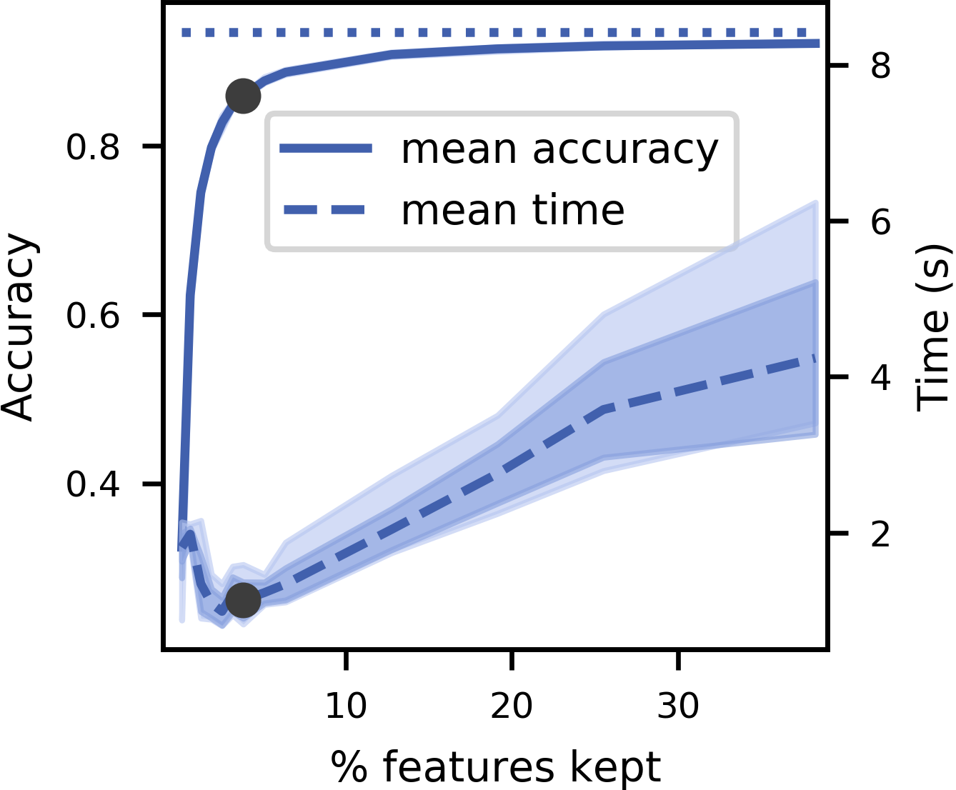
Figure 2 shows the accuracy of the SGMM classifier on the subset $\{0,3,9\}$ of the MNIST dataset as a function of the percentage of features preserved. SGMM recovers close to full GMM accuracy with only a small number of features in a fraction of the time. For instance, at the gray dot, SGMM with $3.82\%$ of the features preserved (30 out of 784) achieves a mean accuracy of $0.86$ ($92\%$ of the accuracy with all features) in $12.9\%$ of the computation time. We further note that there is almost no variance in the accuracy over multiple trials, a consequence of preconditioning that we also observed in our sparsified $k$-means classifier [3].

IV-B Small Cluster Recovery

Figure 3: Small cluster recovery using spherical SGMM.

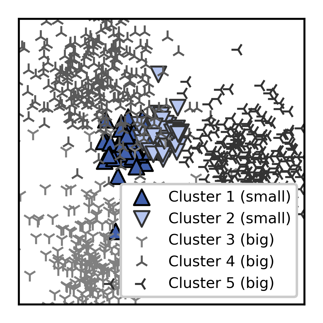
In a regime where clusters have very different sizes, both in the sense of variance and number of points, GMM (even with spherical covariance) can significantly outperform $k$-means. Figure 3 shows an example in which where SGMM correctly identifies two small clusters from three large ones with $98.5\%$ accuracy while $k$-means was unable to recover the clusters ($14.5\%$) accuracy. Data drawn from five $20$-dimensional Gaussians, embedded into $100$-dimensional space, with $\left\lVert\mathbf{S}_{big}\right\rVert_{2}\sim 10\left\lVert\mathbf{S}_{small}\right\rVert_{2}$ and $N_{big}=5\times N_{small}=250$.

IV-C One-Pass Recovery of Means

The fact that we resample the subsampling matrices $\mathbf{R}_{i}$ for each data point $\mathbf{x}_{i}$ is what permits our algorithm to be one-pass. Suppose we wish to approximate a quantity like $\left\lVert\mathbf{x}_{i}-\mathbf{x}_{j}\right\rVert$ in the sparsified regime. The framework we use here would do so by using only the overlapping entries preserved by both $\mathbf{R}_{i}$ and $\mathbf{R}_{j}$. In the event that there is no overlap, we cannot estimate such a quantity. We may introduce a parameter $Q_{S}\in\{0,1,\ldots,Q\}$ indicating how many of the $Q$ features must overlap between all data points. To do so in practice we sample $Q_{S}$ indices once during the sparsification in algorithm 1, and then sample $Q-Q_{S}$ for each $\mathbf{R}_{i}$ subsampling matrix.

Figure 4: Dependence of one-pass mean estimates on the number of shared features $Q_{S}$ in the sparsification. SGMM run on the subset $\{0,3,9\}$ of MNIST with $Q=10$; spherical covariances.

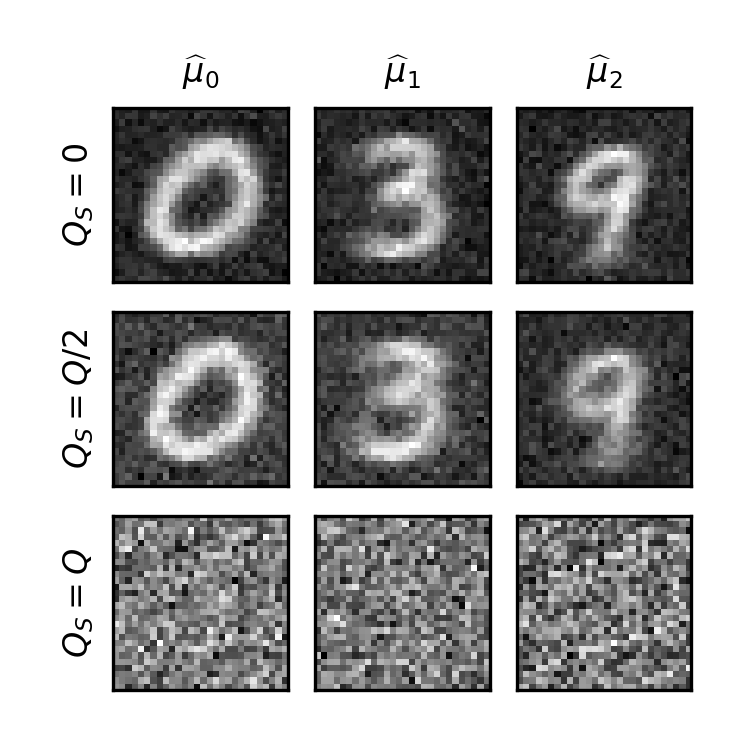
Figure 4 shows the means obtained from the SGMM algorithm applied to the MMIST subset of $\{0,3,9\}$ using three different values of $Q_{S}$. In the first row, $Q=0$, meaning that we do not enforce any overlap (though it may occur by chance), as in algorithm (2). In the second row we have set $Q_{S}=Q/2$, so that half of the features are shared between all data points. The means are noisier, because a pixel is now half as likely to be preserved under sparsification given that it is not one of the $Q_{S}$ features saved for all $\mathbf{x}_{i}$. Finally, in the third row we show the means when we set $Q_{S}=Q$; i.e., the classical random projection regime. The cluster assignments are accurate, but the dense means are meaningless in this regime without a second pass through the data (see Section II-A for further discussion).

V Conclusions

The sparsified Gaussian mixture model is an efficient clustering algorithm that reduces the storage and computational cost of Gaussian mixtures while still being one-pass. After paying an upfront cost of $\mathcal{O}(NP\log P)$ to precondition the data, SGMM compresses $N$ samples from $P$ to $Q$ dimensions, and with diagonal or spherical covariances, fits $K$ clusters in $\mathcal{O}(KNQ)$ time per EM iteration.

References

- [1] A. K. Jain, “Data clustering: 50 years beyond K-means,” Pattern Recognition Letters, vol. 31, no. 8, pp. 651–666, 2010.
- [2] S. Muthukrishnan, Data Streams: Algorithms and Applications. Breda, The Netherlands: Now Publishers, 2005.
- [3] F. Pourkamali-Anaraki and S. Becker, “Preconditioned data sparsification for big data with applications to PCA and K-means,” IEEE Transactions on Information Theory, vol. 63, no. 5, pp. 2954–2974, 2017.
- [4] K. Murphy, Machine Learning: A Probabilistic Perspective. Cambridge, MA: The MIT Press, 2012.
- [5] W. B. Johnson and J. Lindenstrauss, “Extensions of Lipschitz mappings into a Hilbert space,” Contemporary Mathematics, vol. 26, pp. 189–206, 1984.
- [6] N. Ailon and B. Chazelle, “The fast Johnson-Lindenstrauss transform and approximate nearest neighbors,” SIAM Journal on Computing, vol. 39, no. 1, pp. 302–322, 2009.
- [7] E. Candès and M. Wakin, “An introduction to compressive sampling,” IEEE Signal Processing Magazine, vol. 25, no. 2, pp. 21–30, 2008.
- [8] D. Achlioptas, “Database-friendly random projections: Johnson-Lindenstrauss with binary coins,” Journal of Computer and System Sciences, vol. 66, no. 4, pp. 671–687, 2003.
- [9] N. Halko, P.-G. Martinsson, and J. A. Tropp, “Finding structure with randomness: Probabilistic algorithms for constructing approximate matrix decompositions,” SIAM Review, vol. 53, no. 2, pp. 217–288, 2011.
- [10] D. P. Woodruff, “Sketching as a tool for numerical linear algebra,” Foundations and Trends in Theoretical Computer Science, vol. 10, no. 1-2, pp. 1–157, 2014.
- [11] C. Boutsidis, A. Zouzias, M. W. Mahoney, and P. Drineas, “Randomized dimensionality reduction for -means clustering,” IEEE Transactions on Information Theory, vol. 61, no. 2, pp. 1045–1062, 2015.
- [12] M. B. Cohen, S. Elder, C. Musco, C. Musco, and M. Persu, “Dimensionality reduction for k-means clustering and low rank approximation,” in Proceedings of the 47th Annual ACM Symposium on Theory of Computing (STOC), 2015, pp. 163–172.
- [13] K. L. Clarkson and D. P. Woodruff, “Numerical linear algebra in the streaming model,” in Proceedings of the 41st Annual ACM Symposium on Theory of Computing (STOC), 2009, pp. 205–214.
- [14] J. Nelson and H. L. Nguyen, “Lower bounds for oblivious subspace embeddings,” in Automata, Languages, and Programming - 41st International Colloquium (ICALP), 2014, pp. 883–894.
- [15] C. Boutsidis, A. Zouzias, and P. Drineas, “Random Projections for k-means clustering,” in Proceeding of the 23rd Annual Neural Information Processing Systems Conference (NIPS), 2010.
- [16] H. Reboredo, F. Renna, R. Calderbank, and M. R. Rodrigues, “Projections designs for compressive classification,” in Proceedings of the 1st Annual IEEE Global Conference on Signal and Information Processing (GlobalSIP), 2013, pp. 1029–1032.
- [17] J. A. Tropp, A. Yurtsever, M. Udell, and V. Cevher, “Practical sketching algorithms for low-rank matrix approximation,” SIAM Journal on Matrix Analysis and Applications, vol. 38, no. 4, pp. 1454–1485, 2017.
- [18] L. Becchetti, M. Bury, V. Cohen-Addad, F. Grandoni, and C. Schwiegelshohn, “Oblivious dimension reduction for k-means: Beyond subspaces and the Johnson-Lindenstrauss lemma,” in Proceedings of the 51st Annual ACM Symposium on Theory of Computing (STOC), 2019, pp. 1039–1050.
- [19] J. A. Tropp, A. Yurtsever, M. Udell, and V. Cevher, “Streaming low-rank matrix approximation with an application to scientific simulation,” SIAM Journal on Scientific Computing, vol. 41, no. 4, pp. A2430–A2463, 2019.
- [20] T. S. Jayram and D. Woodruff, “Optimal bounds for Johnson-Lindenstrauss transforms and streaming problems with sub-constant error,” ACM Transactions on Algorithms (TALG), vol. 9, no. 3, 2013.
- [21] N. Alon and B. Klartag, “Optimal compression of approximate inner products and dimension reduction,” in Proceedings of the 58th Annual IEEE Symposium on Foundations of Computer Science (FOCS), 2017, pp. 639–650.
- [22] A. Andoni, P. Indyk, and M. Pǎtraşcu, “On the optimality of the dimensionality reduction method,” in Proceedings of the 47th Annual IEEE Symposium on Foundations of Computer Science (FOCS), 2006, pp. 449–458.
- [23] K. G. Larsen and J. Nelson, “Optimality of the Johnson-Lindenstrauss lemma,” in Proceedings of the 58th Annual IEEE Symposium on Foundations of Computer Science (FOCS), 2017, pp. 633–638.
- [24] D. M. Kane and J. Nelson, “Sparser Johnson-Lindenstrauss transforms,” Journal of the ACM, vol. 61, no. 1, pp. 1–23, 2014.
- [25] T. T. Do, L. Gan, N. H. Nguyen, and T. D. Tran, “Fast and efficient compressive sensing using structurally random matrices,” IEEE Transactions on Signal Processing, vol. 60, no. 1, pp. 139–154, 2012.
- [26] D. Arthur and S. Vassilvitskii, “K-means++: The advantages of careful seeding,” in Proceedings of the 18th Annual ACM-SIAM Symposium on Discrete Algorithms (SODA), 2007, pp. 1027–1025.