Scalable Grouped Gaussian Processes via Direct Cholesky Functional Representations

Abstract

We consider multi-task regression models where observations are assumed to be a linear combination of several latent node and weight functions, all drawn from Gaussian process (GP) priors that allow nonzero covariance between grouped latent functions. We show that when these grouped functions are conditionally independent given a group-dependent pivot, it is possible to parameterize the prior through sparse Cholesky factors directly, hence avoiding their computation during inference. Furthermore, we establish that kernels that are multiplicatively separable over input points give rise to such sparse parameterizations naturally without any additional assumptions. Finally, we extend the use of these sparse structures to approximate posteriors within variational inference, further improving scalability on the number of functions. We test our approach on multi-task datasets concerning distributed solar forecasting and show that it outperforms several multi-task GP baselines and that our sparse specifications achieve the same or better accuracy than non-sparse counterparts.

1 Introduction

Gaussian process (gp) models are a flexible nonparametric Bayesian approach that can be applied to various problems such as regression and classification [24] and have been extended to numerous multivariate and multi-task problems including spatial and spatio-temporal contexts [7]. Multi-task gp methods have been developed along several lines (see e.g. [3] for a review) including mixing approaches that combine multiple latent univariate gps via linear or nonlinear mixing to predict multiple related tasks [37, 10, 5, 30, 18, 14]. To maintain scalability in multi-task mixing models, various constraints have been employed. In particular, latent gps may be constrained to be statistically independent as in [37, 11] or covarying with constrained kernel structures to allow algebraic efficiencies as in [10, 5].

In this paper we consider the multi-task setting where subsets of latent functions in Gaussian process regression networks (gprn; [37]) covary within a constrained structure. We build upon the grouped Gaussian process (ggp) approach of [10], where groups of latent functions may covary arbitrarily with a separable kernel structure. Posterior estimation in this ggp framework, as originally proposed in [10], is underpinned by variational inference based on inducing variables [31] and its stochastic optimization extension [17], hence it should be inherently scalable to a large number of observations. However, both the time and space complexity deteriorate significantly when considering a large number of tasks, due to the assumed grouping structure.

Therefore, to address the above limitation, we consider the case where grouped functions are conditionally independent given a specific group-dependent pivot function. We exploit this structure in the prior and in the approximate posterior within a variational inference framework to develop an efficient inference algorithm for the ggp model. Our approach outperforms competitive multi-task baselines and is significantly more efficient (in time and memory) than its non-sparse counterpart. Our specific contributions are given below.

Direct sparse Cholesky functional representation: We show that when the grouped functions in a ggp model are conditionally independent given a group-dependent pivot, it is possible to parameterize the prior through sparse Cholesky factors directly, hence avoiding their computation during inference. We refer to these factors as Cholesky functions as, for a given kernel, they allow us to operate in the Cholesky factorization space directly as a function of the data and the gp hyper-parameters.

Exact construction of sparse Cholesky functionals: We establish for the first time (to the best of our knowledge) that kernels that are multiplicatively separable over input points give rise to such sparse parameterizations naturally without any additional assumptions. This enables direct construction of sparse Cholesky factors without resorting to iterative routines that are inherently costly and unstable, potentially increasing the scope for such kernels to be adopted in other machine learning settings and applications.

Sparse approximate posteriors: Finally, we extend the use of sparse structures to the corresponding approximate distributions within a variational inference framework. The required expectations over these distributions are neatly estimated using a simple but effective ‘indirect’ sampling approach, which further improves scalability on the number of functions.

Experiments: Our approach is driven by the problem of forecasting solar power output at multiple sites. We apply our ggp model and sparse inference framework to this problem using two real multi-task datasets, showing that it outperforms competitive multi-task benchmarks and achieve the same or better forecast performance than non-sparse counterparts in significantly less time.

2 Multi-task gp regression

A Gaussian process (gp; [24]) is formally defined as a distribution over functions such that $f(\mathbf{x})\sim\mathcal{GP}(\mu(\mathbf{x}),\kappa(\mathbf{x},\mathbf{x}^{\prime}))$ is a Gaussian process with mean function $\mu(\mathbf{x})$ and covariance function $\kappa(\mathbf{x},\mathbf{x}^{\prime})$ iff any subset of function values $f(\mathbf{x}_{1}),f(\mathbf{x}_{2}),\ldots,f({\mathbf{x}_{N}})$ follows a Gaussian distribution with mean $\boldsymbol{\mu}$ and covariance $\mathbf{K}$, which are obtained by evaluating the corresponding mean function and covariance function at the input points $\mathbf{X}=\{\mathbf{x}_{1},\ldots,\mathbf{x}_{N}\}$.

In this paper we consider a form of multi-task gp regression where multiple outputs are modeled as a linear combination of node and weight functions, each of which is a gp. Data is of the form $\mathcal{D}=\{\mathbf{X}\in\mathbb{R}^{N\times D},\mathbf{Y}\in\mathbb{R}^{N\times P}\}$ where each $\mathbf{x}_{(n)}$ in $\mathbf{X}$ is a $D$-dimensional vector of input features and each $\mathbf{y}_{(n)}$ in $\mathbf{Y}$ is a $P$-dimensional vector of task outputs. We consider the grouped Gaussian process (ggp)model of [10] who place a prior over $Q$ latent gp functions $\mathbf{F}=\{f_{j}(\mathbf{x})\}_{j=1}^{Q}$ such that arbitrary, non-overlapping subsets (‘groups’) of latent functions may have nonzero covariance.

We denote arbitrarily chosen subsets in $\mathbf{F}$ as $\mathbf{F}_{r}\in\mathbb{R}^{N\times Q_{r}},r=1,\ldots,R$, where $R$ is the total number of groups. For each group the number of latent functions within is denoted $Q_{r}$ (group size) such that $\sum_{r=1}^{R}Q_{r}=Q$. In the gp each group is comprised of latent functions $\mathbf{F}_{r}=\{f_{j}\}_{j\in\text{ group }r}$ and the covariance between two functions is non-zero iff the corresponding processes belong to the same group. This leads to a prior over functions given by

$$p(\mathbf{F}|\boldsymbol{\theta})=\prod_{r=1}^{R}p(\mathbf{F}_{r}|\boldsymbol{\theta}_{r})=\prod_{r=1}^{R}\mathcal{N}(\mathbf{F}_{r};\mathbf{0},\mathbf{K}_{ff}^{r}),$$ (1)

where $\mathbf{K}_{ff}^{r}\in\mathbb{R}^{NQ_{r}\times NQ_{r}}$ is the covariance matrix generated by the group kernel function $\kappa_{r}(f_{j}(\mathbf{x}),f_{j^{\prime}}(\mathbf{x}^{\prime}))$, which evaluates the covariance of functions $f_{j}$ and $f_{j^{\prime}}$ at the locations $\mathbf{x}$ and $\mathbf{x}^{\prime}$, respectively. $\kappa_{r}(f_{j}(\mathbf{x}),f_{j^{\prime}}(\mathbf{x}^{\prime}))=0$ iff $f_{j}$ and $f_{j^{\prime}}$ do not belong to the same group $r$.

Correlations between outputs are modeled as in the Gaussian process regression network (gprn) likelihood of [37], where $\mathbf{f}_{(n)}$ is a $Q$-dimensional vector of latent function values at time $n$ and

$$p(\mathbf{Y}|\mathbf{F},\boldsymbol{\phi})=\prod_{n=1}^{N}p(\mathbf{y}_{(n)}|\mathbf{f}_{(n)},\boldsymbol{\phi})\\ =\prod_{n=1}^{N}\mathcal{N}(\mathbf{y}_{(n)};\mathbf{W}_{(n)}\mathbf{g}_{(n)},\mathbf{\Sigma}_{y})\text{.}$$

Here we define $\mathbf{W}$ and $\mathbf{G}$ subsets of $\mathbf{F}$ formed by gathering $PQ_{g}$ and $Q_{g}$ functions in $\mathbf{F}$, respectively, with $Q_{g}(P+1)=Q$, $\boldsymbol{\phi}=\mathbf{\Sigma}_{y}$, $\mathbf{f}_{(n)}=\{\mathbf{W}_{(n)},\mathbf{g}_{(n)}\}$ and $\mathbf{\Sigma}_{y}$ is a diagonal matrix. $P$-dimensional outputs are constructed at $\mathbf{x}_{(n)}$ as the product of a $P\times Q_{g}$ matrix of weight functions, $\mathbf{W}_{(n)}$, and $Q_{g}$-dimensional vector of node functions $\mathbf{g}_{(n)}$. Partitions of $\mathbf{F}$ with respect to $\mathbf{W}$ and $\mathbf{G}$ need not align with partitions into groups $\mathbf{F}_{r}$. Hence grouping in the prior can be independent of the likelihood definition and, for brevity, inference is presented below simply in terms of $\mathbf{F}$ and $\mathbf{F}_{r}$ rather than $\mathbf{W}$ and $\mathbf{G}$.

To maintain scalability of the approach, we consider separable kernels of the form $\kappa_{r}(f_{j}(\mathbf{x}),f_{j^{\prime}}(\mathbf{x}^{\prime}))=\kappa_{r}(\mathbf{x},\mathbf{x}^{\prime})\kappa_{r}(\mathbf{h}_{j},\mathbf{h}_{j^{\prime}})$, where for each group $Q_{r}$ vectors $\mathbf{h}\in H$ form a feature matrix $\mathbf{H}_{r}\in\mathbb{R}^{Q_{r}\times H}$ that governs covariance across functions $f_{j}\in\mathbf{F}_{r}$. Group covariance $\mathbf{K}_{ff}^{r}=\mathbf{K}_{\mathbf{h}\mathbf{h}}^{r}\otimes\mathbf{K}_{\mathbf{x}\mathbf{x}}^{r}$ thus decomposes into $\mathbf{K}_{\mathbf{x}\mathbf{x}}^{r}\in\mathbb{R}^{N\times N}$ and $\mathbf{K}_{\mathbf{h}\mathbf{h}}^{r}\in\mathbb{R}^{Q_{r}\times Q_{r}}$.

In this paper we propose sparse forms of $\mathbf{K}_{\mathbf{h}\mathbf{h}}^{r}$ arising from a constrained form of cross-function covariance, whereby functions within a group are conditionally independent given a group ‘pivot’ latent function. By exploiting conditional independence constraints that can reasonably fit with spatio-temporal applications such as distributed solar prediction (rationale are discussed in the supplement, §F), it is possible to dramatically reduce the complexity of the gp with respect to group size.

3 Sparse multi-task model

In this section we describe the main assumptions on the task-dependent covariance of our sparse ggp model that will yield significant computational gains over the original ggp. The starting point is that of conditional independence across functions given a group-pivot latent function.

3.1 Conditional independence

When variables are jointly normally distributed and subsets of these variables are conditionally independent, their multivariate normal distribution is known to have certain useful properties. Suppose variables $\mathbf{F}_{r}=f_{1},f_{2},\ldots,f_{Q_{r}}$ are jointly normally distributed with covariance $\mathbf{K}$ (subscripts on $\mathbf{K}$ are dropped for ease of exposition), and suppose that, given some variable $f_{k}$, the remaining variables are conditionally independent. That is,

$$\mathbf{F}_{r}\sim\mathcal{N}(\mu,\mathbf{K})\quad\text{ and }\quad f_{i}\perp f_{j}\,|\,f_{k},\qquad\forall\quad i,j\neq k,\quad i\neq j,$$ (2)

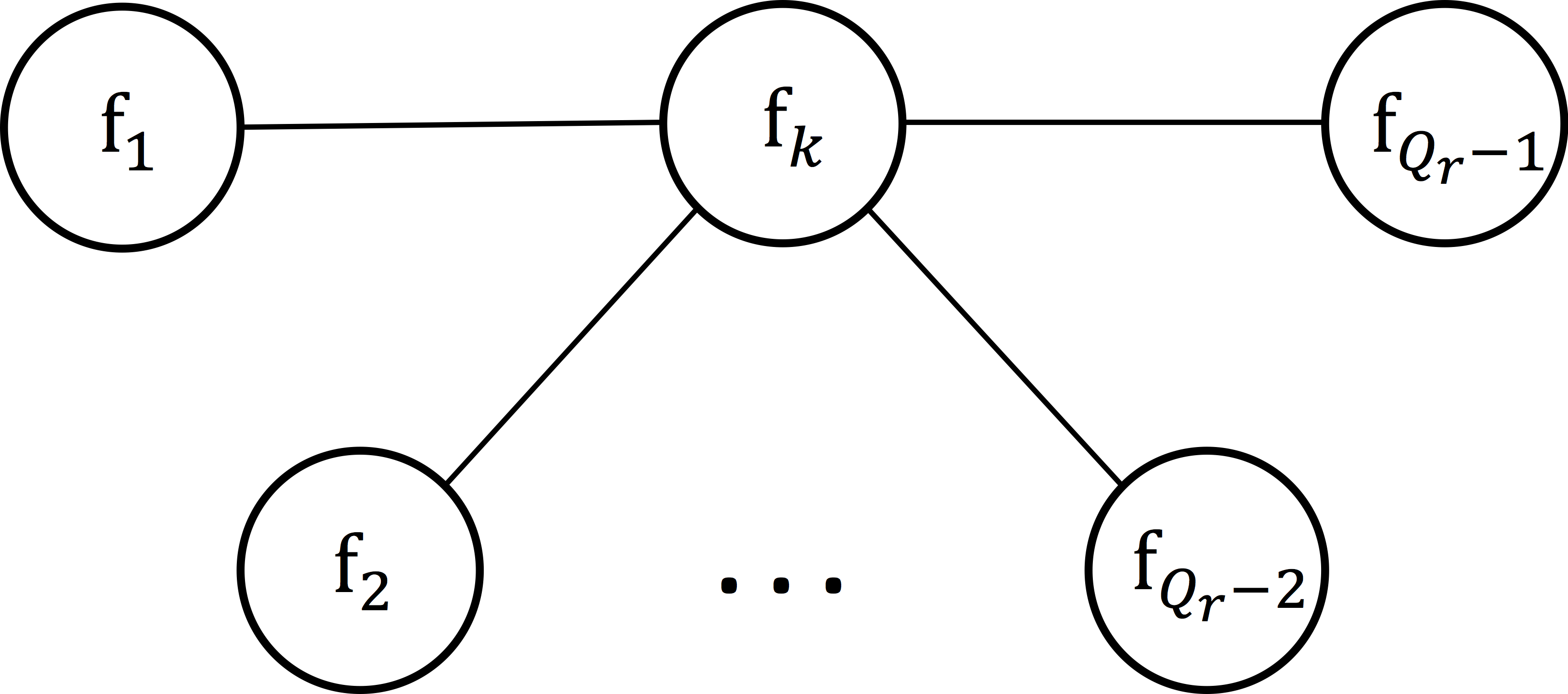
where $f_{i}\perp f_{j}\,|\,f_{k}$ denotes independence of $f_{i}$ and $f_{j}$ given $f_{k}$. This joint distribution can be represented as a ‘star’ or ‘tree’ undirected graphical model, where $f_{k}$ can be conceived as a ‘pivot’ variable connecting all other variables (see Figure 2 in the supplement).

Where variables are jointly distributed according to (2), known, sparse expressions for the Cholesky factor and inverse covariance, that allow direct construction of these matrices, can be obtained analytically [29, 28, 34]. For $i,j\neq k$, $i\neq j$, the covariance element $\mathbf{K}_{i,j}=Cov(f_{i},f_{j})$ is given by

$$\mathbf{K}_{i,j}=\mathbf{K}_{i,k}\mathbf{K}_{k,k}^{-1}\mathbf{K}_{k,j}\iff f_{i}\perp f_{j}\,|\,f_{k}\text{ , }\text{leading to}\quad\mathbf{\Phi}_{i,j}=0\text{ }\text{ and }\mathbf{\Lambda}_{i,j}=0,$$ (3)

where $\mathbf{\Lambda}$ and $\mathbf{\Phi}$ are the precision matrix and lower triangular Cholesky factor of $\mathbf{K}$.

Moreover, nonzero elements of $\mathbf{\Lambda}$ and $\mathbf{\Phi}$ have a known form (see [29, 28] for a useful summary). Without loss of generality, where $f_{2},\ldots,f_{Q_{r}}$ are conditionally independent given $f_{1}$, the precision matrix takes a known winged-diagonal form (see the supplement). Of key importance for our model, the associated Cholesky lower triangular factor $\mathbf{\Phi}$ also has a known, sparse form where $\mathbf{\Phi}_{11}=\textrm{Chol}(\mathbf{K}_{11})$, $\mathbf{\Phi}_{i1}=\mathbf{K}_{i1}(\mathbf{\Phi}_{11})^{-1},i=2,\ldots,Q_{r}$ and $\mathbf{\Phi}_{ii}=\textrm{Chol}(\mathbf{K}_{ii.1})$, $i=2,\dots,Q_{r}$, and $\mathbf{K}_{ii.1}=\mathbf{K}_{ii}-\mathbf{K}_{i1}\mathbf{K}_{11}^{-1}\mathbf{K}_{1i},\quad i=2,\ldots,Q_{r}$, and all other elements are zero. $\textrm{Chol}(\cdot)$ denotes the Cholesky factorization of the given argument.

3.2 Sparse Gaussian process

Let $f(\mathbf{h})$ be drawn from a Gaussian process, $f(\mathbf{h})\sim\mathcal{GP}(\mathbf{0},\kappa(\mathbf{h},\mathbf{h}^{\prime}))$ and assume that $f(\mathbf{h}_{i})\perp f(\mathbf{h}_{j})\quad\lvert\quad f(\mathbf{h}_{k})$ for some $i,j\neq k,i\neq j$. Thus, the properties of multivariate Gaussians above imply the constrained covariance form

$$\kappa(\mathbf{h}_{i},\mathbf{h}_{j}) \equiv\kappa(\mathbf{h}_{i},\mathbf{h}_{k})\kappa(\mathbf{h}_{k},\mathbf{h}_{k})^{-1}\kappa(\mathbf{h}_{k},\mathbf{h}_{j}).$$ (4)

Again without loss of generality, setting $k=1$ and $i=2,\ldots,Q_{r}$ yields a sparse form of the Cholesky factor where

$$\mathbf{\Phi}_{11}=\mathrm{Chol}(\kappa_{11}),\quad\mathbf{\Phi}_{i1}=\kappa_{i1}(\mathbf{\Phi}_{11})^{-1},\quad\text{and}\quad\mathbf{\Phi}_{ii}=\mathrm{Chol}(\kappa_{ii}-\kappa_{i1}\kappa_{11}^{-1}\kappa_{1i}).$$ (5)

This form has several useful characteristics. Computation involves only univariate operations, meaning that $\mathrm{Chol}(\cdot)=\sqrt{(\cdot)}$, $(\mathbf{\Phi}_{11})^{-1}=\frac{1}{\mathbf{\Phi}_{11}}$ and $\kappa_{11}^{-1}=\frac{1}{\kappa_{11}}$. Since there are $2Q_{r}-1$ nonzero terms, complexity of both computation and storage is $\mathcal{O}(Q_{r})$ rather than the more general $\mathcal{O}(Q_{r}^{3})$ and $\mathcal{O}(Q_{r}^{2})$. Computation involving univariate operations only also allows direct control over numerical stability of the factorization.

In addition, the sparse form can be decomposed as two sparse matrices with a single nonzero column and nonzero diagonal respectively, i.e.

$$\mathbf{\Phi}=[\mathbf{\Phi}_{.1},\mathbf{0}_{1},\ldots,\mathbf{0}_{Q_{r}-1}]+\mathrm{diag}(0,\mathbf{\Phi}_{22},\ldots,\mathbf{\Phi}_{Q_{r}Q_{r}}),$$ (6)

where $[\cdot]$ is the concatenation of the first column of $\mathbf{\Phi}$ ($\mathbf{\Phi}_{.1}$) and $Q_{r}-1$ zero column vectors with length $Q_{r}$, and $\mathrm{diag}(\cdot)$ is the diagonal matrix with diagonal elements $(0,\mathbf{\Phi}_{22},\ldots,\mathbf{\Phi}_{Q_{r}Q_{r}})$. In practice, this means matrix operations can be evaluated using efficient vector-broadcasting, rather than matrix multiplication, routines.

To the best of our knowledge, direct construction of sparse Cholesky factors using explicit expressions as above has not been employed in Gaussian process models. Rather, where constrained covariance forms such as given at (2) are used, including in sparse methods discussed at §6, it is in the context of prediction on test points that are conditionally independent given some inducing set of variables or latent functions (see e.g. [22]).

3.2.1 Exact implicit sparsity in gp priors

In some spatio-temporal settings it may be reasonable to explicitly impose the constraint at (4), which we term ‘explicit’ sparsity. In other cases, construction of a Gram matrix, associated Cholesky factor and inverse using general routines and using (3) – (5) are equivalent. This is due to certain kernels implicitly giving rise to the identity in (4). Where kernels can be expressed as products of real-valued functions of $\mathbf{h}_{i}$ and $\mathbf{h}_{j}$, i.e. assuming $\kappa(\mathbf{h}_{i},\mathbf{h}_{j})=\phi(\mathbf{h}_{i})\psi(\mathbf{h}_{j})$, and assuming the inverses ($\phi(\mathbf{h}_{i})^{-1}$, $\psi(\mathbf{h}_{j})^{-1}$) are defined for all $\mathbf{h}_{i},\mathbf{h}_{j}\in\mathbf{H}$, kernels give rise to this identity (see the supplement for details). The requirement for symmetry in Mercer kernels (see e.g. [15]) requires $\kappa(\mathbf{h}_{i},\mathbf{h}_{j})=\kappa(\mathbf{h}_{j},\mathbf{h}_{i})$, implying $\phi(\mathbf{h}_{i})\psi(\mathbf{h}_{j})=\phi(\mathbf{h}_{j})\psi(\mathbf{h}_{i})$ for all $\mathbf{h}_{i},\mathbf{h}_{j}\in\mathbf{H}$, however we note that functions ($\phi(\mathbf{h})$, $\psi(\mathbf{h})$) need not be identical for (4) to hold.

Trivially, multiplicative kernels comprised of kernel functions that have the property at (4) retain this property. Thus Gram matrices that can be expressed as the Hadamard product of matrices constructed via kernel functions of this type also retain the properties at (3). Kernels that meet this criterion include constant kernels, polynomial kernels in one dimension, dot product wavelet kernels, and separable stationary kernels (see [15]). All these kernels decompose multiplicatively into real valued functions of inputs points $\mathbf{h}_{i}$ and $\mathbf{h}_{j}$ in a straightforward way.

3.2.2 Properties of implicitly sparse kernels

Direct decomposition: When kernels decompose multiplicatively for any points $\mathbf{h}_{i}$, $\mathbf{h}_{j}$ and $\mathbf{h}_{k}$, the Cholesky has the form defined by (5). The Cholesky can be expressed and directly constructed in this way because the relationship holds for any three points. Therefore any point can be assigned as the ‘pivot’ point $\kappa_{11}$ and pairwise covariances between any other two points can be expressed in terms of covariances with $\kappa_{11}$.

Degeneracy: A corollary of this, however, is that where (4) holds, only one point on the diagonal is nonzero, $\Phi_{11}$, since for all other points, $\kappa_{ii}-\kappa_{i1}\kappa_{11}^{-1}\kappa_{1i}=0$ (from (5)), implying that the gp is degenerate. The kernels listed above that decompose multiplicatively are positive semi-definite, as opposed to strictly positive definite, Mercer kernels [24, 39]. One of the criticisms of the degenerate model is that, for distance-based kernels, predictive variance at new points reduces with distance from observed points and in the limit can be zero [21].

Avoiding degeneracy in ggp models: Issues around degeneracy are avoided in our framework for two reasons. Firstly, use of a sparse construction is limited to $\mathbf{K}_{\mathbf{h}\mathbf{h}}^{r}$. In essence, the model induces sparsity over tasks rather than observations. Under multi-task latent function mixing approaches, including ggp, it is generally the case that predictions are not made on new tasks. As such, there is no degeneration over test points since locations across latent functions are fixed for training and test observations. Secondly, as is common practice we add a Kronecker delta kernel (see [15]) to diagonal elements, however excluding the pivot which maintains the model as an exact gp prior without losing the direct Cholesky construction. This is possible because, for $\mathbf{K}_{\mathbf{h}\mathbf{h}}^{r}$, the pivot input point does not change. Pivot choice is discussed at §5 and in the supplement.

4 Inference

Inference for the sparse ggp follows the sparse variational approach of [31] and extended by [11, 10] where the prior at (1) is augmented with inducing variables $\{\mathbf{u}_{r}\}_{r=1}^{R}$, drawn from the same gp priors as $\mathbf{F}_{r}$ at $M$ inducing points $\mathbf{Z}_{r}$ in the same space as $\mathbf{X}$, giving

$$p(\mathbf{u}|\boldsymbol{\theta})=\prod_{r=1}^{R}\mathcal{N}(\mathbf{u}_{r};\mathbf{0},\mathbf{K}_{uu}^{r})\quad\text{ and }\quad p(\mathbf{F}|\mathbf{u})=\prod_{r=1}^{R}\mathcal{N}(\mathbf{F}_{r};\tilde{\boldsymbol{\mu}}_{r},\widetilde{\mathbf{K}}_{r}),$$ (7)

where $\tilde{\boldsymbol{\mu}}_{r}=\mathbf{A}_{r}\mathbf{u}_{r}$, $\widetilde{\mathbf{K}}_{r}=\mathbf{K}_{ff}^{r}-\mathbf{A}_{r}\mathbf{K}_{uf}^{r}$ and $\mathbf{A}_{r}=\mathbf{K}_{fu}^{r}(\mathbf{K}_{uu}^{r})^{-1}=\mathbf{I}_{Qr}\otimes\mathbf{K}_{\mathbf{x}\mathbf{z}}^{r}(\mathbf{K}_{\mathbf{z}\mathbf{z}}^{r})^{-1}$. $\mathbf{K}_{uu}^{r}\in\mathbb{R}^{MQ_{r}\times MQ_{r}}$ is governed by $\kappa_{r}(f_{j}(\mathbf{x}),f_{j^{\prime}}(\mathbf{x}^{\prime}))$ evaluated over $\mathbf{Z}_{r}$, $\mathbf{H}_{r}$, similarly yielding the decomposition $\mathbf{K}_{uu}^{r}=\mathbf{K}_{\mathbf{h}\mathbf{h}}^{r}\otimes\mathbf{K}_{\mathbf{z}\mathbf{z}}^{r}$. The joint posterior distribution over $\{\mathbf{F},\mathbf{u}\}$ is approximated by variational inference with

$$p(\mathbf{F},\mathbf{u}|\mathbf{Y})\approx q(\mathbf{F},\mathbf{u}|\boldsymbol{\lambda})\stackrel{{\scriptstyle\text{\tiny def}}}{{=}}p(\mathbf{F}|\mathbf{u})q(\mathbf{u}|\boldsymbol{\lambda})\quad\text{with}\quad q(\mathbf{u}|\boldsymbol{\lambda})=\sum_{k=1}^{K}\pi_{k}\prod_{r=1}^{r}q_{k}(\mathbf{u}_{r}|\boldsymbol{\lambda}_{kr}),$$ (8)

where $q_{k}(\mathbf{u}_{r}|\boldsymbol{\lambda}_{kr})=\mathcal{N}(\mathbf{u}_{r};\mathbf{m}_{kr},\mathbf{S}_{kr})$ and $\boldsymbol{\lambda}_{kr}=\{\mathbf{m}_{kr},\mathbf{S}_{kr},\pi_{k}\}$. $\mathbf{m}_{kr}$ and $\mathbf{S}_{kr}$ are, respectively, a freely parameterized mean vector and covariance matrix and $\pi_{k}$ are mixture weights. Prediction for a new point $\mathbf{y}_{\star}$ given $\mathbf{x}_{\star}$ is computed as the expectation over the variational posterior for the new point:

$$p(\mathbf{y}_{\star}|\mathbf{x}_{\star}) =\sum_{k=1}^{K}\pi_{k}\int p(\mathbf{y}_{\star}|\mathbf{f}_{\star})q_{k}(\mathbf{f}_{\star}|\boldsymbol{\lambda}_{k})\text{d}\mathbf{F}_{\star},$$ (9)

where $q_{k}(\mathbf{f}_{\star}|\boldsymbol{\lambda}_{k})$ is defined as for $q_{k(n)}(\mathbf{f}_{(n)}|\boldsymbol{\lambda}_{k})$ below (see §4.1). The expectation in Eq. (9) is estimated via Monte Carlo (mc) sampling: $\mathbb{E}_{p(\mathbf{y}_{\star}|\mathbf{x}_{\star})}{\left[\mathbf{y}_{\star}\right]}\approx\frac{1}{S}\sum_{s=1}^{S}\mathbf{W}_{\star}^{s}\mathbf{g}_{\star}^{s},$ where $\{\mathbf{W}_{\star}^{s}\text{,}\mathbf{g}_{\star}^{s}\}=\mathbf{f}_{\star}^{s}$ are samples from $q_{k}(\mathbf{f}_{\star}|\boldsymbol{\lambda}_{k})$. To estimate the posterior parameters we optimize the evidence lower bound (elbo) defined as $\mathcal{L}_{\text{elbo}}\stackrel{{\scriptstyle\text{\tiny def}}}{{=}}\mathcal{L}_{\text{ent}}+\mathcal{L}_{\text{cross}}+\mathcal{L}_{\text{ell}}$ where $\mathcal{L}_{\text{ent}}$, $\mathcal{L}_{\text{cross}}$ and $\mathcal{L}_{\text{ell}}$ are entropy, cross entropy and expected log likelihood terms, respectively. Derivations of the general expressions for the gp model and elbo can be found at [10, 11]. In evaluating the efficiency of our approach we consider both a diagonal and Kronecker structure for $\mathbf{S}_{kr}$. We define the Kronecker specification as $\mathbf{S}_{kr}=\mathbf{S}_{krb}\otimes\mathbf{S}_{krw}$ where $\mathbf{S}_{krb}\in\mathbb{R}^{Q_{r}\times Q_{r}}$ and $\mathbf{S}_{krw}\in\mathbb{R}^{M\times M}$ are both sparse, freely parameterized matrices that heuristically correspond to ‘between’ and ‘within’ covariance components. Sparsity is induced via Cholesky factors of the form at (5).

4.1 Computational gains and indirect sampling

The corresponding components of the elbo are as follows,

$$\mathcal{L}_{\text{ent}}\geq-\sum_{k=1}^{K}\pi_{k}\log\sum_{l=1}^{K}\pi_{l}\prod_{r=1}^{R}\mathcal{N}(\mathbf{m}_{kr};\mathbf{m}_{lr},\mathbf{S}_{kr}+\mathbf{S}_{lr})\stackrel{{\scriptstyle\text{\tiny def}}}{{=}}\widehat{\mathcal{L}_{\text{ent}}},$$ (10)

$$\mathcal{L}_{\text{cross}}(\boldsymbol{\lambda}) =-\frac{1}{2}\sum_{k=1}^{K}\pi_{k}\sum_{r=1}^{R}\left[c_{r}+\log\left\lvert\mathbf{K}_{uu}^{r}\right\rvert+\mathbf{m}_{kr}^{\prime}(\mathbf{K}_{uu}^{r})^{-1}\mathbf{m}_{kr}+\mbox{ \rm tr }((\mathbf{K}_{uu}^{r})^{-1}\mathbf{S}_{kr})\right],$$ (11)

$$\mathcal{L}_{\text{ell}}(\boldsymbol{\lambda}) =\sum_{n=1}^{N}\mathbb{E}_{q_{(n)}(\mathbf{f}_{(n)}|\boldsymbol{\lambda})}{\left[\log p(\mathbf{y}_{(n)}|\mathbf{f}_{(n)},\boldsymbol{\phi})\right]},$$ (12)

where $c_{r}=M_{r}\log 2\pi$ and $\widehat{\mathcal{L}_{\text{ent}}}$ is used instead of $\mathcal{L}_{\text{ent}}$. The main computational gains, following the efficiencies due to the Kronecker factorization, arise from the sparsification of the prior and the approximate posterior. Indeed, we can show that costly algebraic operations on the matrices $\mathbf{S}_{kr}$ and $\mathbf{K}_{\mathbf{h}\mathbf{h}}^{r}$ (obtained from the Kronecker factorization of $\mathbf{K}_{uu}^{r}$) such as log determinants and inverses are reduced from $\mathcal{O}(Q_{r}^{3})$ to $\mathcal{O}(Q_{r})$ for the entropy and the cross-entropy terms in Eqs. (10) and (11).

However, for the expected log likelihood (ell) term in Eq. (12) we still need to sample from the marginal posterior $q_{(n)}(\mathbf{f}_{(n)}|\boldsymbol{\lambda})$ which is done by sampling from component group mixture posteriors i.e. $q_{k(n)}(\mathbf{f}_{(n)Q_{r}}|\boldsymbol{\lambda}_{kr})=\mathcal{N}(\mathbf{b}_{kr(n)},\mathbf{\Sigma}_{kr(n)})$ with mean and covariance expressions given by $\mathbf{b}_{kr(n)}=\mathbf{A}_{r(n)}\mathbf{m}_{kr}$ and $\mathbf{\Sigma}_{kr(n)}=\widetilde{\mathbf{K}}_{r(n)}+\mathbf{A}_{r(n)}\mathbf{S}_{kr}\mathbf{A}_{r(n)}^{\prime}$, where $\widetilde{\mathbf{K}}_{r}$ and $\mathbf{A}_{r}$ are defined as in (7) (detailed expressions are provided in the supplement, §E). Naïvely, this is $\mathcal{O}(Q_{r}^{3})$. We address this issue by ‘indirect sampling’, i.e. drawing independent samples from two distributions specified as $\mathcal{N}(\mathbf{0},\widetilde{\mathbf{K}}_{r(n)})$ and $\mathcal{N}(\mathbf{b}_{kr(n)},\mathbf{A}_{r(n)}\mathbf{S}_{kr}\mathbf{A}_{r(n)}^{\prime})$, and summing these to return samples from $\mathcal{N}(\mathbf{b}_{kr(n)},\mathbf{\Sigma}_{kr(n)})$, hence reducing the time complexity to $\mathcal{O}(Q_{r})$. Similarly, these savings for the ell apply to predictions as obtained from Eq. (9). Finally, there are significant gains from the proposed sparsification and indirect sampling method in terms of memory complexity, going from $\mathcal{O}(Q_{r}^{2})$ to $\mathcal{O}(Q_{r})$. Full complexity analysis is given in the supplement, §E.

5 Application to solar photovoltaic (pv) forecasting

We test the sparse ggp model on solar forecasting applications, where tasks are solar sites and the modelling goal is to jointly predict power output at all sites at each test time point $n$. The sparse ggp model for solar follows the approach in [10] where, for $P$ tasks, there are $P$ latent node functions, meaning $Q_{g}(P+1)=Q$. Latent weight functions are grouped according to rows of $\mathbf{W}_{(n)}$ while latent node functions are assumed to be independent. Thus, predicted output at site $i$, $\mathbf{y}_{(n)i}$, is a linear combination of (site-associated) node functions. Spatial features, $\mathbf{h}_{j}=(latitude_{j},longitude_{j}),j=1,\ldots,Q_{r}$, populate the cross function feature matrix $\mathbf{H}_{r}$ for every group. We test three forms of $\mathbf{K}_{\mathbf{h}\mathbf{h}}^{r}$ Cholesky factors: an implicitly sparse form via multiplicatively separable kernels; an explicitly sparse form where the equality in (4) is imposed rather than naturally arising; and a sparse, freely parameterized factor. Group pivot functions are set as the diagonal elements of $\mathbf{W}_{(n)}$ (see the supplement, §F).

5.1 Experiments

Data are five minute average power output between 7am and 7pm. We test our model using two datasets (with $P=25$ and $P=50$). The first dataset consists of 25 proximate sites over 45 days in Spring with 105,000 (57,000) observations for training (testing). The second dataset consists of 50 proximate sites in a different location and season (Autumn) with 210,000 (114,000) observations in total for training (testing). We forecast power output 15 minutes ahead at each site over the test period.

For $P=25$ we evaluate performance relative to the general ggp and three classes of non-ggp benchmarks: the linear coregional model (lcm), gprn and multi-task model with task-specific features (mtg) of [6]. In addition, we test a general ggp model with full, freely parameterized cross site covariance. For $P=50$, we evaluate sparse models using Kronecker posteriors against non ggp benchmarks. However, other ggp models could not be estimated under the same computational constraints. We consider the root mean squared error (rmse), mean absolute error (mae), negative log predictive density (nlpd), average model rank (m-rank) and forecast variance (f-var) to evaluate the performance of all methods. Full details of the experimental set-up are given in the supplement, §F.

5.1.1 Results

Results for all models are reported at Table 1with further results available in the supplement (§G). For $P=25$ forecast accuracy of sparse and general ggp models is comparable. Results for sparse and non sparse ggp models differ by less than a percentage point on rmse and mae, while nlpd results are slightly more variable.

Table 1: Forecast accuracy and variance of ggp, sparse ggp and benchmark models. Results shown for Kronecker posteriors with $K=1$ for Adelaide ($P=25$) and Sydney ($P=50$) datasets. Results are reported for best performing gprn and lcm benchmarks (based on rmse) and for lcm where $Q_{g}=P$. All metrics are losses, i.e. the lower the better.

P = 25
Kronecker	rmse	mae	nlpd	m-rank	f-var
ggp	0.343	0.213	0.382	4.3	0.117
ggp (free)	0.344	0.213	0.384	5.3	0.112
Sparse ggp (implicit)	0.342	0.213	0.414	4.7	0.120
Sparse ggp (explicit)	0.341	0.214	0.374	2.7	0.114
Sparse ggp (free)	0.344	0.216	0.378	7.0	0.111
lcm ($Q_{g}=P$)	0.375	0.236	0.583	16.0	0.180
lcm ($Q_{g}=4$)	0.367	0.240	0.475	14.7	0.147
gprn ($Q_{g}=2$)	0.342	0.214	0.446	5.7	0.150
mtg	0.381	0.237	0.502	16.3	0.170
P = 50
Kronecker	rmse	mae	nlpd	m-rank	f-var
Sparse ggp (implicit)	0.421	0.254	0.622	1.0	0.159
Sparse ggp (explicit)	0.421	0.257	0.626	2.3	0.141
Sparse ggp (free)	0.423	0.258	0.625	2.7	0.139
lcm ($Q_{g}=P$)	0.451	0.283	0.807	5.3	0.211
gprn ($Q_{g}=2$)	0.428	0.263	0.664	4.0	0.185
mtg	0.483	0.297	0.741	5.7	0.211

For $P=25$, accuracy is comparable for ggp and gprn on mae and rmse, however ggp based models perform significantly better than benchmarks on nlpd. The lcm and mtg perform relatively poorly on all measures. Mean forecast variance was also found to be significantly lower (28 percent on average) under ggp models relative to benchmark models. For $P=50$, sparse ggp models outperform benchmark models on all accuracy and variance measures.

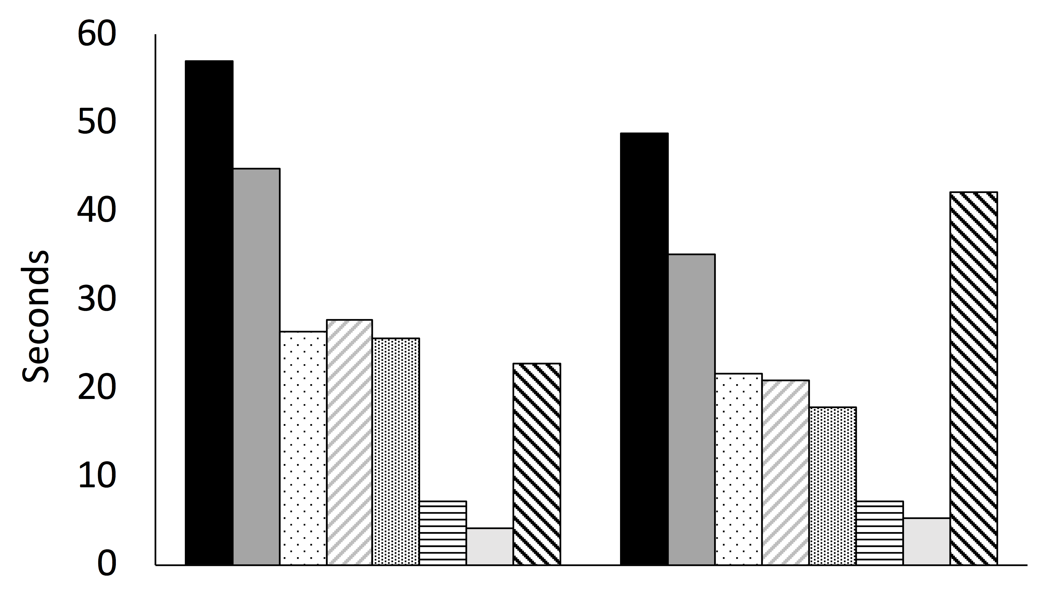
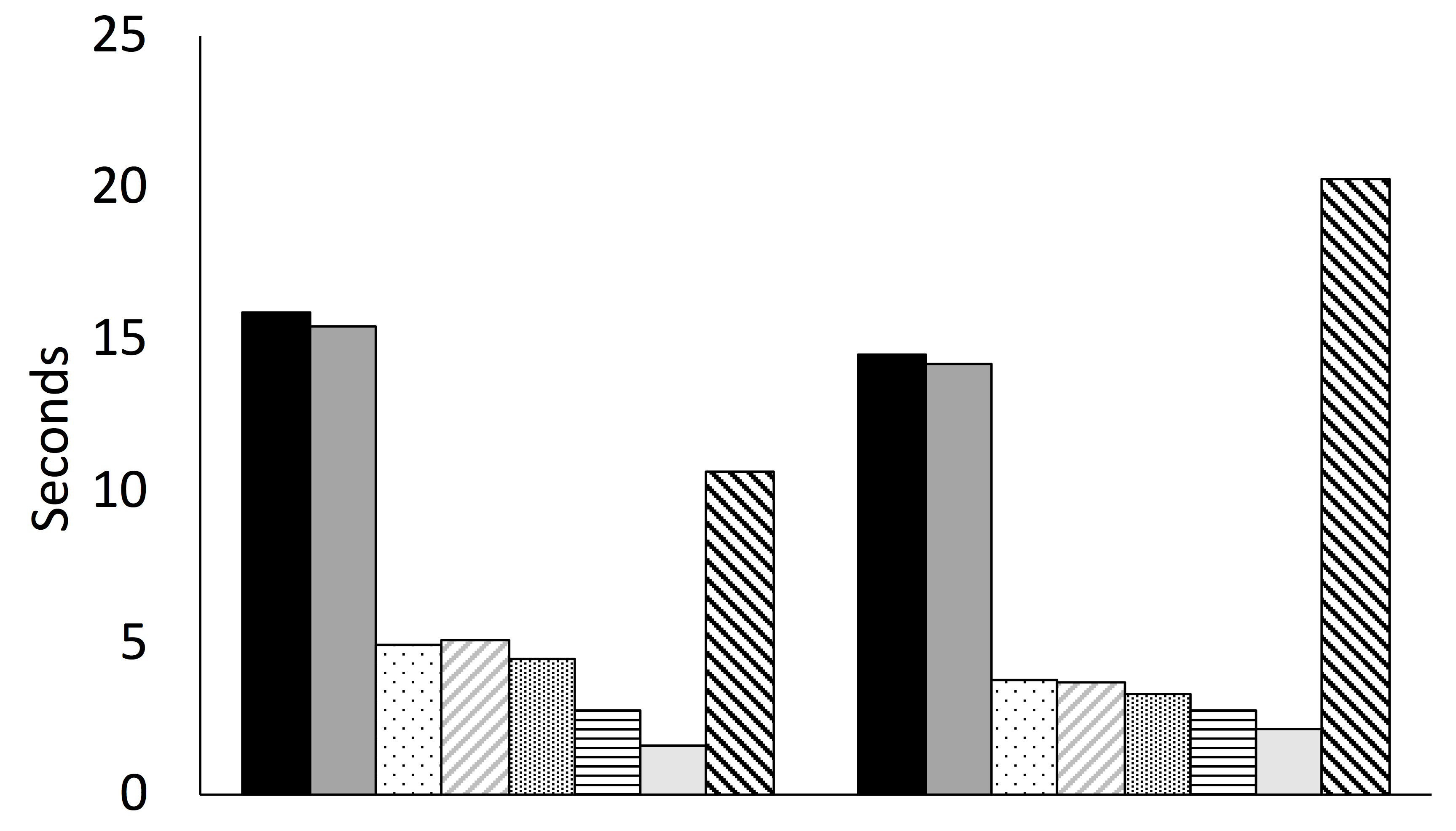
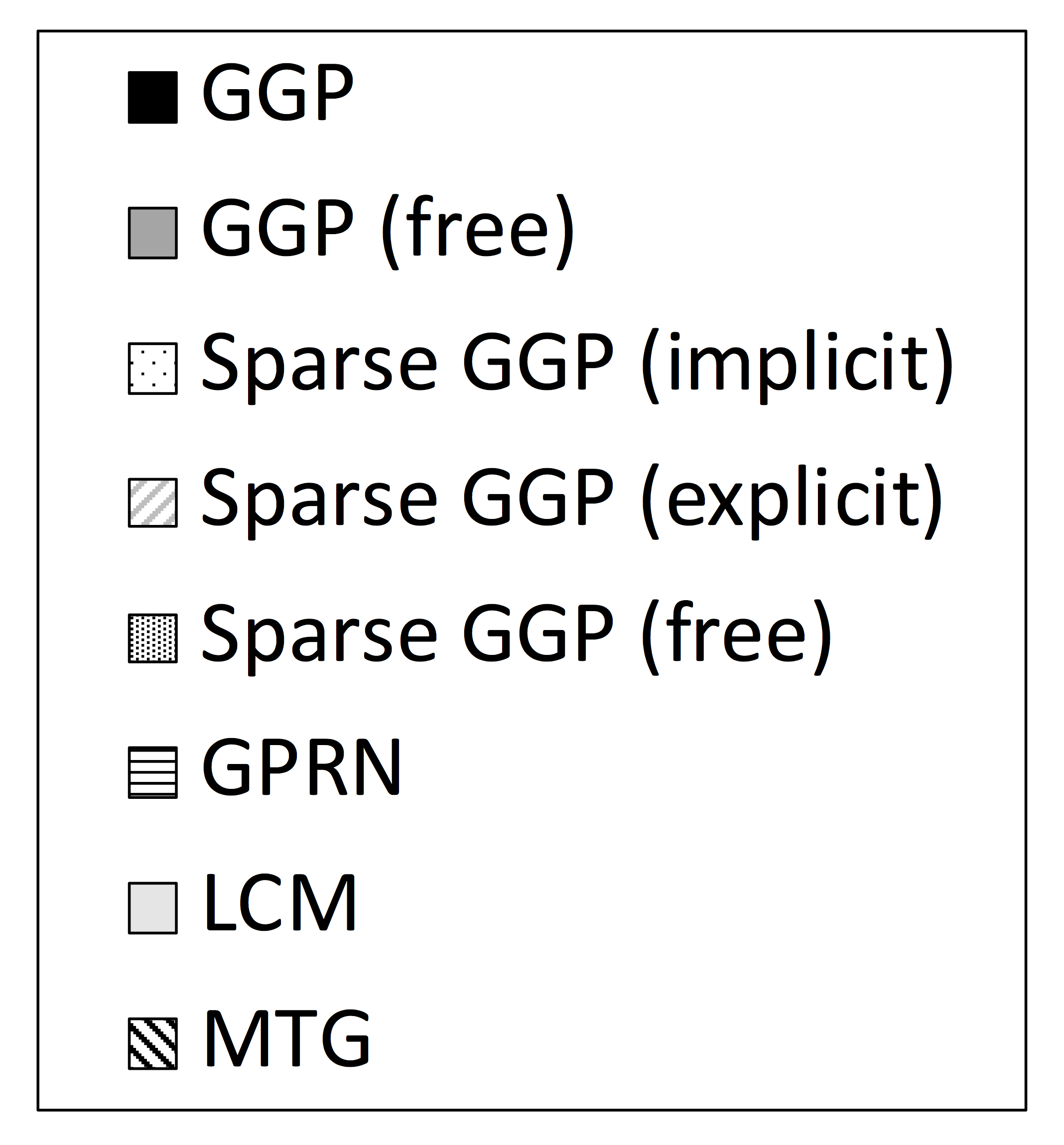
Computation times are shown at Figure 1 for sparse versus general ggp models and benchmark models. Results confirm that sparse ggp models have substantially lower time costs than general counterparts; step time and elbo computation time are decreased by 49 to 57 percent and 43 to 57 percent respectively, with Kronecker posteriors showing greater reductions than diagonal posteriors (55 versus 50 percent, respectively, on average). The most substantial improvements, however, are for prediction, where sparse models are three to four times faster over the full test set. Further, mean sparse model prediction time scales close to linearly between $P=25$ (at 3.6 seconds) and $P=50$ (at 8.5 seconds). Computation time for step and elbo for $P=50$ (not shown) scales at a higher-than-linear rate overall (on average three times the cost of comparable models for $P=25$), which we mainly attribute to the grouping structure selected.

We also find that, for the same prior, average time cost is always lower under the Kronecker posterior, consistent with their lower complexity as discussed in the supplement, E. Further, freely parameterized ggp models have lower time costs than ‘standard’ counterparts reflecting the lower complexity of operations on $\mathbf{K}_{\mathbf{h}\mathbf{h}}^{r}$ elements ($\mathcal{O}(1)$ versus $\mathcal{O}(H)$ for explicitly defined kernels).

Diagonal	Kronecker	Diagonal	Kronecker

Figure 1: Computation times for ggp versus sparse ggp models ($P=25$) for diagonal and Kronecker posteriors. Left: Average time to compute the full evidence lower bound. Right: Average time to compute predictions over the full test set.

Time costs for gprn and lcm benchmarks are lower again than sparse ggp based models, in the order of 1.3 to 6.3 times faster per operation. The mtg, however, has very low step time (up to 27 times faster than sparse ggp models) and comparable time cost for elbo in the diagonal case but substantially poorer results for elbo and prediction computation times for remaining tests.

6 Related work

The problem of forecasting local solar output in the short term is of significant interest for the purpose of distributed grid control and household energy management [32, 35]. A number of studies confirm that exploiting spatial dependencies between proximate sites can yield significant gains in forecast accuracy and stability [10, 38]. More importantly, inherent to this application is the need for modeling uncertainty in a flexible and principled way (see e.g. [4]), hence our motivation to use gps.

The literature on scalable inference for gp models is vast and the reader is referred to [20] for a comprehensive review of this area. Here we focus on closely related approaches to ours. Early methods adopt low-rank decompositions or assume some kind of conditional independence [26, 22], with later studies extending these conditional independence ideas to convolutional multi-task models [1, 2]. Nowadays it is widely recognized that the inducing variable framework of [31], made scalable by [17], is one of the de facto standards for scalable gps. However, other approaches such as those based on random feature expansions of the covariance function remain relevant [16, 8]. Another idea that has been used in sparse methods is that of structured inputs, e.g. regular one-dimensional gridded inputs, which induce Toeplitz matrices with sparse inverses [36].

Other methods make use of conditional independence relationships arising naturally in Gaussian Markov random fields, particularly the integrated nested Laplace approximation (inla) of [25]. These approaches assume a more general conditional independence structure arising from the Markov blanket property. Closely related to methods inducing conditional independence, several recent techniques consider low-rank approximations in inducing point frameworks [13, 9]. In fact, [13] use a low-rank pivoted Cholesky approximation with pre-conditioning for various gp models including sparse methods. Other approaches using low-rank approximations based on spectral methods have also been proposed as in [27, 12].

While sparse variational and other recent low-rank gp methods have provided substantial gains in scalability in recent years, as general approaches they do not necessarily exploit efficiencies where sparse, cross-task covariances can be specified a priori as may be possible in well understood spatio-temporal problems. Finally, given the increasing capabilities of current GPU-based computing architectures, it is not surprising to see very recent developments to solve gp regression exactly in very large datasets [33].

7 Discussion

We have shown that by exploiting known properties of multivariate Gaussians and conditional independence across latent functions, it is possible to significantly improve the scalability of multi task mixing models with respect to the number of functions. We have applied this approach to the problem of solar forecasting at multiple distributed sites using two large multi task datasets and demonstrated that both spatially driven and freely parameterized sparse cross function covariance structures can be exploited to achieve faster learning and prediction without sacrificing forecast performance. In particular the cost of prediction is dramatically reduced and shown to be linear in the number of grouped latent functions.

Appendix A An example of a sparse ggp prior

Figure 2: Example of Undirected Graphical Model in Star Formation for $\mathbf{F}_{r}=(f_{1},f_{2},\ldots,f_{Q_{r}})^{\prime}$.

Appendix B Code and Datasets

We have made our implementation of the sparse and non sparse ggp models available at the Github repository: https://github.com/spggp/sparse-ggp.

The repository also contains datasets used in reported experiments and example scripts for execution.

Appendix C Expressions for multivariate Gaussian precision matrix

The precision matrix from [28, 34], has a sparse, winged diagonal form

$$\mathbf{\Lambda}=\begin{bmatrix}\mathbf{\Lambda}_{11}&\mathbf{\Lambda}_{21}^{\prime}&\mathbf{\Lambda}_{31}^{\prime}&\cdots&\mathbf{\Lambda}_{Q_{r}1}^{\prime}\\ \mathbf{\Lambda}_{21}&\mathbf{\Lambda}_{22}&0&\cdots&0\\ \mathbf{\Lambda}_{31}&0&\mathbf{\Lambda}_{33}&\cdots&0\\ \vdots&\vdots&\vdots&\ddots&\vdots\\ \mathbf{\Lambda}_{Q_{r}1}&0&0&\cdots&\mathbf{\Lambda}_{Q_{r}Q_{r}}\end{bmatrix}$$

where

$$\mathbf{\Lambda}_{11} =\mathbf{K}_{11}^{-1}+\sum_{i=2}^{Q_{r}}\mathbf{K}_{11}^{-1}\mathbf{K}_{1i}\mathbf{K}_{ii.1}^{-1}\mathbf{K}_{i1}\mathbf{K}_{11}^{-1}$$

$$\mathbf{\Lambda}_{1i} =-\mathbf{K}_{11}^{-1}\mathbf{K}_{1i}\mathbf{K}_{ii.1}^{-1}$$

$$\mathbf{\Lambda}_{ii} =\mathbf{K}_{ii.1}^{-1},\quad\text{where}$$

$$\mathbf{K}_{ii.1} =\mathbf{K}_{ii}-\mathbf{K}_{i1}\mathbf{K}_{11}^{-1}\mathbf{K}_{1i},\quad i=2,\ldots,Q_{r}$$

The sparse Cholesky factor of $\mathbf{K}$ has the form

$$\mathbf{\Phi}=\begin{bmatrix}\mathbf{\Phi}_{11}&0&0&\cdots&0\\ \mathbf{\Phi}_{21}&\mathbf{\Phi}_{22}&0&\cdots&0\\ \mathbf{\Phi}_{31}&0&\mathbf{\Phi}_{33}&\cdots&0\\ \vdots&\vdots&\vdots&\ddots&\vdots\\ \mathbf{\Phi}_{Q_{r}1}&0&0&\cdots&\mathbf{\Phi}_{Q_{r}Q_{r}}\end{bmatrix}$$

where

$$\mathbf{\Phi}_{11} =\mathrm{Chol}(\kappa_{11}),\quad\mathbf{\Phi}_{i1}=\kappa_{i1}(\mathbf{\Phi}_{11})^{-1},\quad\text{and}$$

$$\mathbf{\Phi}_{ii} =\mathrm{Chol}(\kappa_{ii}-\kappa_{i1}\kappa_{11}^{-1}\kappa_{1i}).$$

Appendix D Proof of implicit sparsity in exact gp priors

Construction of a Gram matrix, associated Cholesky factor and inverse using general routines and direct sparse constructions are equivalent where kernels implicitly give rise to the identity where

$$\kappa(\mathbf{h}_{i},\mathbf{h}_{j}) =\kappa(\mathbf{h}_{i},\mathbf{h}_{k})\kappa(\mathbf{h}_{k},\mathbf{h}_{k})^{-1}\kappa(\mathbf{h}_{k},\mathbf{h}_{j})$$

$$\iff f(\mathbf{h}_{i})\perp f(\mathbf{h}_{j})\quad\lvert\quad f(\mathbf{h}_{k})$$ (13)

for any points $\mathbf{h}_{i}$, $\mathbf{h}_{j}$ and $\mathbf{h}_{k}$.

Where kernels can be expressed as products of real-valued functions of $\mathbf{h}_{i}$ and $\mathbf{h}_{j}$, i.e. assuming $\kappa(\mathbf{h}_{i},\mathbf{h}_{j})=\phi(\mathbf{h}_{i})\psi(\mathbf{h}_{j})$, and assuming the inverses ($\phi(\mathbf{h}_{i})^{-1}$, $\psi(\mathbf{h}_{j})^{-1}$) are defined for all $\mathbf{h}_{i},\mathbf{h}_{j}\in\mathbf{H}$, kernels give rise to this identity. To see this, consider a positive semi-definite kernel such that

$$\kappa(\mathbf{h}_{i},\mathbf{h}_{j}) =\phi(\mathbf{h}_{i})\psi(\mathbf{h}_{j})$$

$$\implies\kappa(\mathbf{h}_{k},\mathbf{h}_{k})^{-1} =\phi(\mathbf{h}_{k})^{-1}\psi(\mathbf{h}_{k})^{-1}$$

$$\implies\kappa(\mathbf{h}_{i},\mathbf{h}_{j}) =\phi(\mathbf{h}_{i})\psi(\mathbf{h}_{k})\phi(\mathbf{h}_{k})^{-1}\psi(\mathbf{h}_{k})^{-1}$$

$$\times\phi(\mathbf{h}_{k})\psi(\mathbf{h}_{j})$$

$$=\kappa(\mathbf{h}_{i},\mathbf{h}_{k})\kappa(\mathbf{h}_{k},\mathbf{h}_{k})^{-1}\kappa(\mathbf{h}_{k},\mathbf{h}_{j})$$ (14)

Kernels of this form are valid, positive semi-definite kernels so long as the properties of symmetry and positive semi-definiteness are satisfied. Symmetry implies $\kappa(\mathbf{h}_{i},\mathbf{h}_{j})=\kappa(\mathbf{h}_{j},\mathbf{h}_{i})$, implying $\phi(\mathbf{h}_{i})\psi(\mathbf{h}_{j})=\phi(\mathbf{h}_{j})\psi(\mathbf{h}_{i})$ for all $\mathbf{h}_{i},\mathbf{h}_{j}\in\mathbf{H}$. Positive semi-definiteness implies for any examples $\mathbf{h}_{i},\mathbf{h}_{j}$ and any set of real numbers $\lambda_{1},\ldots,\lambda_{l}$, $\sum_{i=1}^{l}\sum_{j=1}^{l}\lambda_{i},\lambda_{j}\kappa(\mathbf{h}_{i},\mathbf{h}_{j})\geq 0$ (see e.g. [15]).

We note that following diagonal correction the implicitly sparse model is no longer invariant to pivot choice, however is still an exact gp when used as in our model (i.e. to characterize cross function covariance in the mixing model). For a collection of random variables to meet the definition of a gp, it is only required that any finite subset of the collection is jointly Gaussian distributed, not precluding finite index sets [24]. This observation also extends to the explicitly sparse case and undefined, freely parameterized case.

Appendix E Computational Complexity

We consider complexity of key terms required for inference and prediction for sparse versus non-sparse models in the following sections, specifically complexity per group of latent functions. In the discussion that follows, it is assumed that $d$-dimensioned matrix inverses can be evaluated with complexity $\mathcal{O}(d^{3})$ in the general case and $\mathcal{O}(d)$ in sparse or diagonal cases due to nonzero elements of sparse matrices growing linearly with $d$ (see §3.1).

Entropy

The entropy component of the elbo is approximated by

$$\mathcal{L}_{\text{ent}}\geq-\sum_{k=1}^{K}\pi_{k}\log\sum_{l=1}^{K}\pi_{l}\mathcal{N}(\mathbf{m}_{k};\mathbf{m}_{l},\mathbf{S}_{k}+\mathbf{S}_{l})\quad\text{with}$$

$$\mathcal{N}(\mathbf{m}_{k};\mathbf{m}_{l},\mathbf{S}_{k}+\mathbf{S}_{l})=\prod_{r=1}^{R}\mathcal{N}(\mathbf{m}_{kr};\mathbf{m}_{lr},\mathbf{S}_{kr}+\mathbf{S}_{lr}).$$ (15)

The normal terms in (15) differ in complexity over posterior forms and whether $l=k$. In the case where $K>1$ and with a Kronecker posterior, both the general and sparse ggp have poor scalability since evaluation requires the log determinant and inverse of $\mathbf{S}_{kr}+\mathbf{S}_{lr}$ with complexity $\mathcal{O}((MQ_{r})^{3})$. Hence, we consider $K=1$ or diagonal posteriors for $K\geq 1$. In the diagonal case time and space complexity is $\mathcal{O}(MQ_{r})$ for sparse and non sparse models ($\mathcal{O}(KMQ_{r})$ for $K>1$).

For the non-diagonal case, the entropy component for each group $r$ reduces to $-\frac{1}{2}(\text{log}\left\lvert 2\mathbf{S}_{kr}\right\rvert)-C$ where $C$ is constant with respect to model parameters. Since the log determinant decomposes as $\text{log}\left\lvert 2\mathbf{S}_{kr}\right\rvert=Q_{r}M\ln 2+M\ln\left\lvert\mathbf{S}_{krb}\right\rvert+Q_{r}\ln\left\lvert\mathbf{S}_{krw}\right\rvert$ evaluation depends only on the diagonal with complexity $\mathcal{O}(Q_{r}+M)$. The cost of storage is $\mathcal{O}(Q_{r}+M)$ versus $\mathcal{O}(Q_{r}^{2}+M^{2})$ for sparse and general cases.

Cross Entropy

$\mathcal{L}_{\text{cross}}$ has several components that differ across sparse and general models, since

$$\mathcal{L}_{\text{cross}}(\boldsymbol{\lambda})=-\frac{1}{2}\sum_{k=1}^{K}\pi_{k}\sum_{r=1}^{R}\left[M_{r}\log(2\pi)+\log\left\lvert\mathbf{K}_{uu}^{r}\right\rvert+\mathbf{m}_{kr}^{\prime}(\mathbf{K}_{uu}^{r})^{-1}\mathbf{m}_{kr}+\mbox{ \rm tr }((\mathbf{K}_{uu}^{r})^{-1}\mathbf{S}_{kr})\right].$$ (16)

Evaluation of $\mathcal{L}_{\text{cross}}$ involves three potentially costly expressions, $\left\lvert\mathbf{K}_{uu}^{r}\right\rvert$, $(\mathbf{K}_{uu}^{r})^{-1}\mathbf{m}_{kr}$ and $\mbox{ \rm tr }((\mathbf{K}_{uu}^{r})^{-1}\mathbf{S}_{kr})$, naively $\mathcal{O}((MQ_{r})^{3})$, considered in turn below.

Log determinant: Similar to the entropy term, the expression $\left\lvert\mathbf{K}_{uu}^{r}\right\rvert$ decomposes to require only the calculation of $\left\lvert\mathbf{K}_{\mathbf{h}\mathbf{h}}^{r}\right\rvert$ and $\left\lvert\mathbf{K}_{\mathbf{z}\mathbf{z}}^{r}\right\rvert$ in $\mathcal{O}(M^{3}+Q_{r}^{3})$ or $\mathcal{O}(M^{3}+Q_{r})$ per group for general and sparse models respectively.

Matrix-vector term: The winged diagonal form of $(\mathbf{K}_{\mathbf{h}\mathbf{h}}^{r})^{-1}$ enables computation of $(\mathbf{K}_{uu}^{r})^{-1}\mathbf{m}_{kr}$ in $\mathcal{O}(M^{3}+Q_{r})$ in the sparse case versus $\mathcal{O}(M^{3}+Q_{r}^{3})$ time in the general case.

Trace term: The trace term involves both prior and posterior covariance matrices. For the Kronecker posterior which allows $\mbox{ \rm tr }((\mathbf{K}_{uu}^{r})^{-1}\mathbf{S}_{kr})=\mbox{ \rm tr }((\mathbf{K}_{\mathbf{h}\mathbf{h}}^{r})^{-1}\mathbf{S}_{krb})\mbox{ \rm tr }((\mathbf{K}_{\mathbf{z}\mathbf{z}}^{r})^{-1}\mathbf{S}_{krw})$ complexity is reduced from $\mathcal{O}(M^{3}+Q_{r}^{3})$ to $\mathcal{O}(Q_{r}+M^{3})$ from the general to sparse. Where $\mathbf{S}_{kr}$ is diagonal, the trace term requires only diagonal elements of $(\mathbf{K}_{\mathbf{h}\mathbf{h}}^{r})^{-1}$, $(\mathbf{K}_{\mathbf{z}\mathbf{z}}^{r})^{-1}$ and $\mathbf{S}_{kr}$. leading to $\mathcal{O}(Q_{r}+M^{3}+MQ_{r})$ versus $\mathcal{O}(Q_{r}^{3}+M^{3}+MQ_{r})$ in the general case.

Expected Log Likelihood

$\mathcal{L}_{\text{ell}}$ is defined as

$$\mathcal{L}_{\text{ell}}(\boldsymbol{\lambda})=\sum_{n=1}^{N}\mathbb{E}_{q_{(n)}(\mathbf{f}_{(n)}|\boldsymbol{\lambda})}{\left[\log p(\mathbf{y}_{(n)}|\mathbf{f}_{(n)},\boldsymbol{\phi})\right]}$$ (17)

where we estimate the expectation in (17) by mc sampling from $q_{(n)}(\mathbf{f}_{(n)}|\boldsymbol{\lambda})$ as discussed below.

E.1 Indirect sampling

Sampling from the posterior distribution of $\mathbf{f}_{(n)}$ and similarly $\mathbf{f}_{\star}$ is required for both $\mathcal{L}_{\text{ell}}$ and prediction. Samples from $q_{(n)}(\mathbf{f}_{(n)}|\boldsymbol{\lambda})$ can be drawn from component group posteriors i.e. $q_{k(n)}(\mathbf{f}_{(n)Q_{r}}|\boldsymbol{\lambda}_{kr})=\mathcal{N}(\mathbf{b}_{kr(n)},\mathbf{\Sigma}_{kr(n)})$ with mean and covariance expressions given by $\mathbf{b}_{kr(n)}=\mathbf{A}_{r(n)}\mathbf{m}_{kr}$ and $\mathbf{\Sigma}_{kr(n)}=\widetilde{\mathbf{K}}_{r(n)}+\mathbf{A}_{r(n)}\mathbf{S}_{kr}\mathbf{A}_{r(n)}^{\prime}$, where

$$\widetilde{\mathbf{K}}_{r(n)} =\mathbf{K}_{\mathbf{h}\mathbf{h}}^{r}\times\left[\kappa_{r}(\mathbf{x}_{(n)},\mathbf{x}_{(n)}\right.$$

$$\left.-\kappa_{r}(\mathbf{x}_{(n)},\mathbf{Z}_{r})(\mathbf{K}_{\mathbf{z}\mathbf{z}}^{r})^{-1}\kappa_{r}(\mathbf{Z}_{r},\mathbf{x}_{(n)})\right]\quad\text{and}$$

$$\mathbf{A}_{r(n)} =\left[\mathbf{I}_{Q_{r}}\otimes\kappa_{r}(\mathbf{x}_{(n)},\mathbf{Z}_{r})(\mathbf{K}_{\mathbf{z}\mathbf{z}}^{r})^{-1}\right]$$

Given a Kronecker posterior the quadratic term simplifies to

$$\mathbf{A}_{r(n)}\mathbf{S}_{kr}\mathbf{A}_{r(n)}^{\prime}=\left[\mathbf{S}_{krb}\otimes\right.$$

$$\left.\kappa_{r}(\mathbf{x}_{(n)},\mathbf{Z}_{r})(\mathbf{K}_{\mathbf{z}\mathbf{z}}^{r})^{-1}\mathbf{S}_{krw}(\mathbf{K}_{\mathbf{z}\mathbf{z}}^{r})^{-1}\kappa_{r}(\mathbf{Z}_{r},\mathbf{x}_{(n)})\right]$$

Direct sampling as in [10] requires factorizing the posterior covariance to obtain a premultiplier $\Psi(\mathbf{\Sigma}_{kr(n)})$ such that $\Psi\Psi^{\prime}=\mathbf{\Sigma}_{kr(n)}$. However, since this differs for each observation the associated cost per group is $\mathcal{O}(NQ_{r}^{3})$, where $N$ is mini-batch size for $\mathcal{L}_{\text{ell}}$ sampling or $N_{test}$ for prediction. We avoid this by making use of known Cholesky factors and sampling from two component distributions using the property that the sum of two independent, normally distributed random variables, $\mathbf{X}\sim\mathcal{N}(\boldsymbol{\mu}_{\mathbf{X}},\Sigma_{\mathbf{X}})$ and $\mathbf{Y}\sim\mathcal{N}(\boldsymbol{\mu}_{\mathbf{Y}},\Sigma_{\mathbf{Y}})$ is also a normally distributed with mean $\boldsymbol{\mu}_{\mathbf{X}}+\boldsymbol{\mu}_{\mathbf{Y}}$ and covariance $\Sigma_{\mathbf{X}}+\Sigma_{\mathbf{Y}}$. We draw independent samples from two distributions specified as $\mathcal{N}(\mathbf{0},\widetilde{\mathbf{K}}_{r(n)})$ and $\mathcal{N}(\mathbf{b}_{kr(n)},\mathbf{A}_{r(n)}\mathbf{S}_{kr}\mathbf{A}_{r(n)}^{\prime})$, and sum these to return samples from $\mathcal{N}(\mathbf{b}_{kr(n)},\mathbf{\Sigma}_{kr(n)})$.

Complexity of factorizations for $\widetilde{\mathbf{K}}_{r(n)}$ and $\mathbf{A}_{r(n)}\mathbf{S}_{kr}\mathbf{A}_{r(n)}^{\prime}$ once obtained differs across variants but where a sparse prior is adopted, is reduced to $\mathcal{O}(NQ_{r})$. Critically, in the sparse case memory complexity is significantly reduced by replacing the premultiplier $\Psi(\widetilde{\mathbf{K}}_{r(n)})$ with vector operations reducing memory complexity from $\mathcal{O}(NQ_{r}^{2})$ to $\mathcal{O}(NQ_{r})$.

The time costs to obtain the quadratic term $\mathbf{A}_{r(n)}\mathbf{S}_{kr}\mathbf{A}_{r(n)}^{\prime}$ are $\mathcal{O}(NM^{2}Q_{r}+M^{3})$, $\mathcal{O}(N(M^{2}+Q_{r}^{2})+M^{3})$ and $\mathcal{O}(N(M^{2}+Q_{r})+M^{3})$ for the diagonal, general Kronecker and sparse Kronecker posteriors respectively. Similarly, the time costs of obtaining $\widetilde{\mathbf{K}}_{r(n)}$ are $\mathcal{O}(N(M^{2}+Q_{r}^{2})+M^{3})$ or $\mathcal{O}(N(M^{2}+Q_{r})+M^{3})$ for the general and sparse priors respectively. Direct sampling would then require combination and factorization of these components in $\mathcal{O}(NQ_{r}^{3})$ time and with $\mathcal{O}(NQ_{r}^{2})$ memory.

Indirect sampling requires factorization of $\widetilde{\mathbf{K}}_{r(n)}$ in $\mathcal{O}(NQ_{r}^{2}+Q_{r}^{3})$ time for general priors and $\mathcal{O}(NQ_{r})$ for sparse priors. Similarly, given a Kronecker posterior, Cholesky factors for the quadratic term can be obtained in $\mathcal{O}(NQ_{r}^{2}+Q_{r}^{3})$ and $\mathcal{O}(NQ_{r})$ for general and sparse specifications, respectively, and $\mathcal{O}(NQ_{r})$ in the diagonal case.

Overall, indirect sampling reduces time, but not memory, complexity relative to direct sampling in the general model. However, by using sparse priors it is possible to achieve significant reductions from the general indirect model. Further gains still are possible if a sparse Kronecker posterior is used in lieu of a diagonal posterior. The last point arises since (broadly speaking) operations involving sparse matrices can exploit decomposition properties of the Kronecker product to achieve linear complexity that is additive, rather than multiplicative, over $M$ and $Q_{r}$. The same observation may be made about complexity reductions in entropy and cross entropy terms. Further details are provided in the supplement.

Appendix F Details of experimental set-up

Three classes of non-ggp benchmark models are considered, the linear coregional model (lcm), gprn and multi-task model with task-specific features (mtg) of [6]. These benchmarks are chosen as they can be implemented in the same inference framework as the ggp and sparse ggp,allowing direct comparison of model performance. For the lcm model, we report two specifications for $P=25$. The first mirrors the ggp with $P=Q_{g}$ -and the second is a lower ranked model with $Q_{g}=5$ ($Q_{g}=4$) for diagonal (Kronecker) posteriors. For $P=50$ we report only the first specification (the best lcm model based on rmse). For the gprn, we report models with $Q_{g}=2$. This was the best performing specification for $P=25$, and the largest value for $Q_{g}$ able to run on the same platform as sparse ggp models.

F.1 Kernels

Kernels for mtg models are defined as $\kappa(f_{j}(\mathbf{x}),f_{j^{\prime}}(\mathbf{x}^{\prime}))=\kappa_{Per.}(t,s)\kappa_{RBF}(\boldsymbol{l}_{jt},\boldsymbol{l}_{j^{\prime}s})\kappa_{RBF-Ep.(2)}(\mathbf{h}_{j},\mathbf{h}_{j^{\prime}})$. For gprn latent functions in a row $\mathbf{W}_{i}$, the kernel is defined as $\kappa_{Per.}(t,s)\kappa_{RBF}(\boldsymbol{l}_{it},\text{ }\boldsymbol{l}_{is})$. For node functions, we use a radial basis kernel with lag features. For lcm $P=Q_{g}$, node functions are defined as combined periodic-radial basis kernels. For lower rank mixing models, we tested two node specifications for $Q_{g}=2,3,4,5$, (a) lags for all sites assigned to each node function, and (b) subsets of lags assigned to node functions based on k-means clustering of lags into $Q_{g}$ groups. Reported benchmarks for lcm use clustered lags, while gprn benchmarks use complete lags per node.

For node functions, $\kappa_{\mathbf{g}_{j}}(\mathbf{x}_{t},\mathbf{x}_{s})$ is a radial basis function kernel on a vector of lagged power features at site $i$, i.e. for site $i$ at time $t$, $\boldsymbol{l}_{i,t}=(y_{i,t},y_{i,t-1})$. For each row-group $r$ in $\mathbf{W}_{(n)}$, $\kappa_{r}(f_{j}(\mathbf{x}),f_{j^{\prime}}(\mathbf{x}^{\prime}))=\kappa_{r}(\mathbf{x},\mathbf{x}^{\prime})\kappa_{r}(\mathbf{h}_{j},\mathbf{h}_{j^{\prime}})$ with $\kappa_{r}(\mathbf{x},\mathbf{x}^{\prime})=\kappa_{Per.}(t,s)\kappa_{RBF}(\boldsymbol{l}_{rt},\boldsymbol{l}_{rs})$, where $\kappa_{Per.}(t,s)$ is a periodic kernel on a time index $t$.

F.2 Solar model variants

Selection of sparsity constraints a priori

Given the spatial nature of covariance between sites and where node functions align with tasks, the weight applied to each node by a given task would be expected to be a function of the (notional) spatial location of the node relative to the target task. We assume that weights are conditionally independent given the weight assigned to the task-associated node for that node. We enforce this constraint for each row-group $i$ of $\mathbf{W}_{(n)}$,

$$\mathbf{W}_{(n)ij}\perp\mathbf{W}_{(n)ik}\quad\lvert\quad\mathbf{W}_{(n)ii}$$ (18)

$j,k\neq i$, $j\neq k$. Since latent function groupings in the ggp framework can be any subset of $\mathbf{F}$ in any order, it is only required that, for sparse inference, latent functions within each group $\mathbf{W}_{(n)i.}$ are ordered such that $\mathbf{W}_{(n)ii}$ acts as the pivot. Within each row of weights, this gives rise to the star configuration for the undirected graphical model (as illustrated at Figure 2 in the supplement), with a single pivot weight function ($\mathbf{W}_{(n)ii}$), and conditionally independent child weight functions corresponding to cross-site nodes ($\mathbf{W}_{(n)ij},j\neq i$).

Cross-function kernel variants

We test three sparse forms of $\mathbf{K}_{\mathbf{h}\mathbf{h}}^{r}$, which we term (a) ‘implicitly sparse’ (sparsity is automatic i.e. implicit in the model due to separable kernel specification as discussed at §3.2.1), (b) ‘explicitly sparse’ (a stationary kernel that does not give rise to automatic sparsity but is used in conjuntion with the constraint in (4) explicitly imposed), and (c) ‘free sparsity’ ($\mathbf{K}_{\mathbf{h}\mathbf{h}}^{r}$ is freely parameterized using $2Q_{r}-1$ parameters for nonzero Cholesky elements and no kernel form is defined).

In the implicitly sparse case, we use a separable, dot product wavelet kernel with Ricker mother wavelet function (see [39]) plus diagonal correction as described at §3.2.1, which we assume to be shared across groups. The full kernel is given by $\kappa_{r(wav.)}+\kappa_{r(diag)}$ and the (full rank) sparse Cholesky can be constructed as in (5) with $\mathbf{\Phi}_{ii}=\sqrt{\kappa_{r(diag)}},i\neq 1$.

For the explicit sparsity case, we use a combined radial basis, Epanechnikov kernel function with the constraint at (4) enforced by setting $Chol(\mathbf{K}_{\mathbf{h}\mathbf{h}}^{r})_{j,k}=0$, $j,k\neq 1$, $j\neq k$. Specifically, $\kappa_{r}(\mathbf{h}_{j},\mathbf{h}_{j^{\prime}})=\kappa_{RBF}(\mathbf{h}_{j},\mathbf{h}_{j^{\prime}})\kappa_{Ep.}(\mathbf{h}_{j},\mathbf{h}_{j^{\prime}})$, $j,j^{\prime}=1\ldots P$.

F.3 Experimental Settings

All models are estimated based on the variational framework explained in §4 with indirect sampling used for both sparse and general models. Starting values for common components were set to be equal across all models and the number of inducing points per group of latent functions is set to approximately standardize computational complexity per iteration relating to $RM^{3}$, using $M=200$ per ggp group as the baseline.

The elbo is iteratively optimized until its relative change over successive epochs is less than $10^{-5}$ up to a maximum of 200 epochs or maximum of 20 hours. Optimization is performed using adam [19] with settings $\{LR=0.005;\beta_{1}=0.09;\beta_{2}=0.99\}$. All data except time index features are normalized prior to optimization. Time and performance measures are captured every five epochs. Timed experimental results reported exclude time required to compute and store the various performance measures during optimization.

Appendix G Additional Experimental Results

Table 2: Forecast accuracy and variance of ggp, sparse ggp and benchmark models. Results shown for diagonal and Kronecker posteriors with $K=1$ for Adelaide ($P=25$) and Sydney ($P=50$) datasets. Results are reported for best performing gprn and lcm benchmarks (based on rmse) and for lcm where $Q_{g}=P$. m-rank is average model rank over accuracy measures (rmse, mae and nlpd).

P = 25
	rmse	mae	nlpd	m-rank	f-var
Diagonal
ggp	0.343	0.216	0.399	7.3	0.121
ggp (free)	0.345	0.215	0.378	7.0	0.116
Sparse ggp (implicit)	0.344	0.217	0.423	10.7	0.124
Sparse ggp (explicit)	0.345	0.215	0.382	7.7	0.115
Sparse ggp (free)	0.343	0.215	0.371	4.7	0.115
lcm ($Q_{g}=P$)	0.371	0.235	0.553	15.0	0.181
lcm ($Q_{g}=5$)	0.366	0.239	0.481	14.3	0.151
gprn ($Q_{g}=2$)	0.344	0.217	0.451	10.7	0.149
mtg	0.381	0.241	0.501	16.7	0.171
Kronecker
ggp	0.343	0.213	0.382	4.3	0.117
ggp (free)	0.344	0.213	0.384	5.3	0.112
Sparse ggp (implicit)	0.342	0.213	0.414	4.7	0.120
Sparse ggp (explicit)	0.341	0.214	0.374	2.7	0.114
Sparse ggp (free)	0.344	0.216	0.378	7.0	0.111
lcm ($Q_{g}=P$)	0.375	0.236	0.583	16.0	0.180
lcm ($Q_{g}=4$)	0.367	0.240	0.475	14.7	0.147
gprn ($Q_{g}=2$)	0.342	0.214	0.446	5.7	0.150
mtg	0.381	0.237	0.502	16.3	0.170
P = 50
Kronecker	rmse	mae	nlpd	m-rank	f-var
Sparse ggp (implicit)	0.421	0.254	0.622	1.0	0.159
Sparse ggp (explicit)	0.421	0.257	0.626	2.3	0.141
Sparse ggp (free)	0.423	0.258	0.625	2.7	0.139
lcm ($Q_{g}=P$)	0.451	0.283	0.807	5.3	0.211
gprn ($Q_{g}=2$)	0.428	0.263	0.664	4.0	0.185
mtg	0.483	0.297	0.741	5.7	0.211

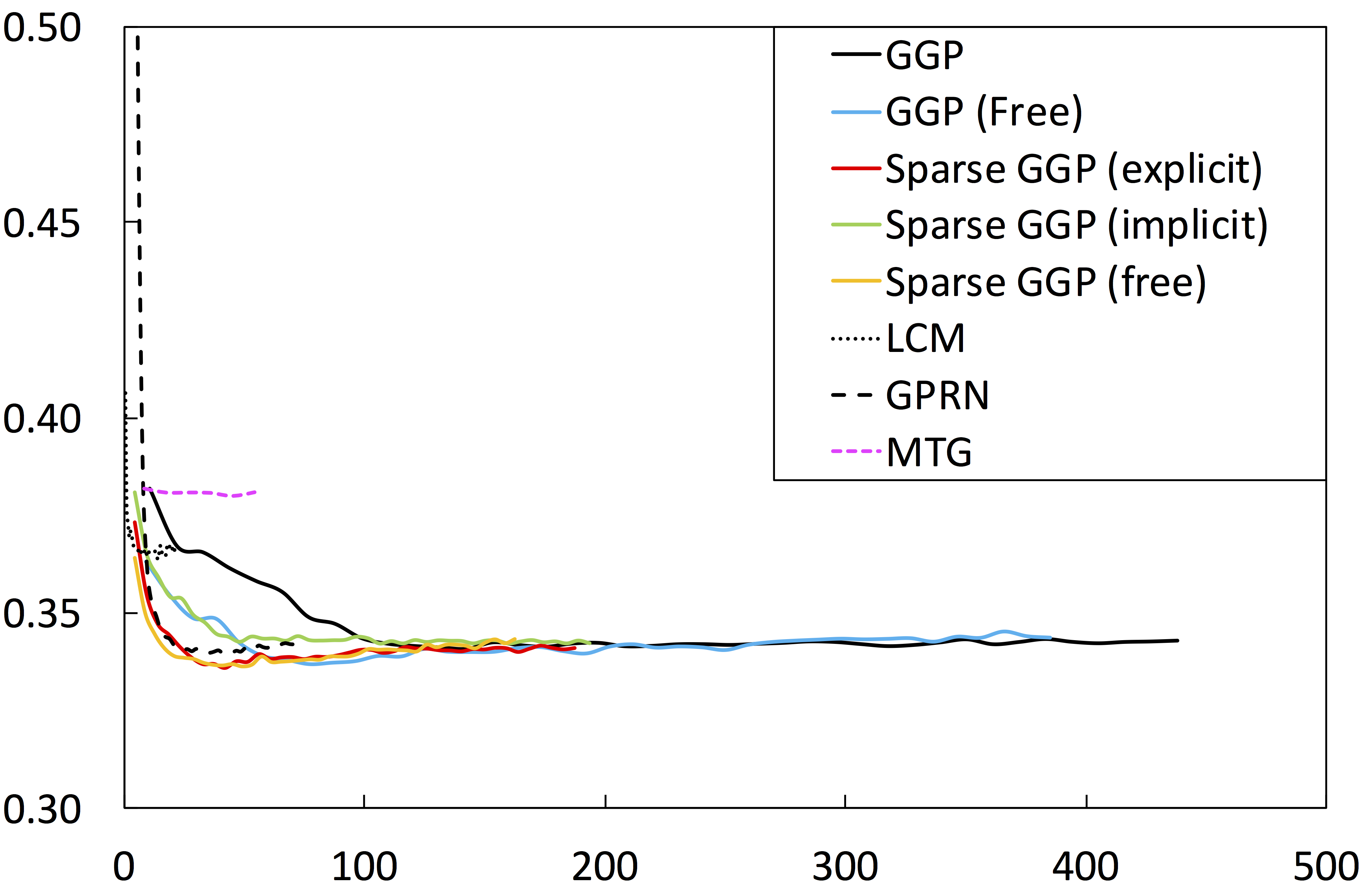
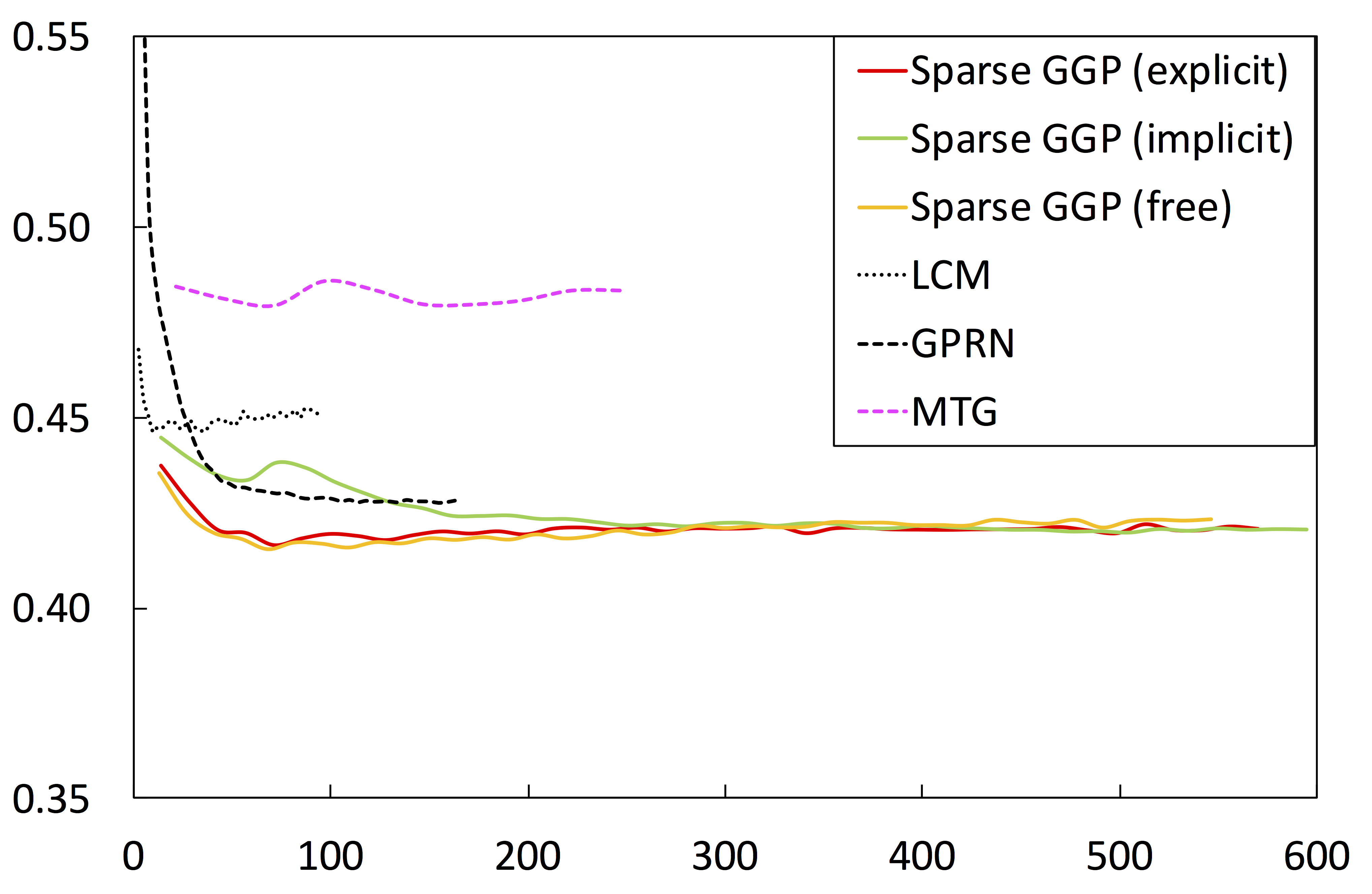
Further experimental results are provided at Table 2. Representative results for forecast accuracy over estimation time for rmse with sparse posterior are shown at Figures 3 and 4. Optimization of benchmark models is faster than ggp based models in some cases, however we also find that performance of ggp models quickly surpasses that of benchmark models. We found rankings in terms of speed at which gains are achieved to be consistent across accuracy measures and posterior specifications. In particular, lcm and gprn achieve their gains quickly as do explicitly sparse and free sparse ggp models, while general ggp models and implicitly sparse ggp models achieve gains more gradually.

Figure 3: rmse over optimization time for $P=25$ with Kronecker posterior.

Figure 4: rmse over optimization time for $P=50$ with Kronecker posterior.

Estimated covariance

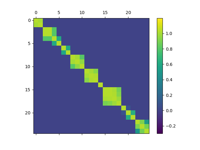
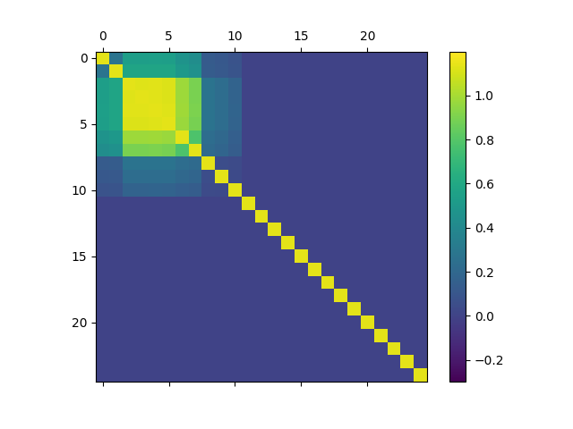
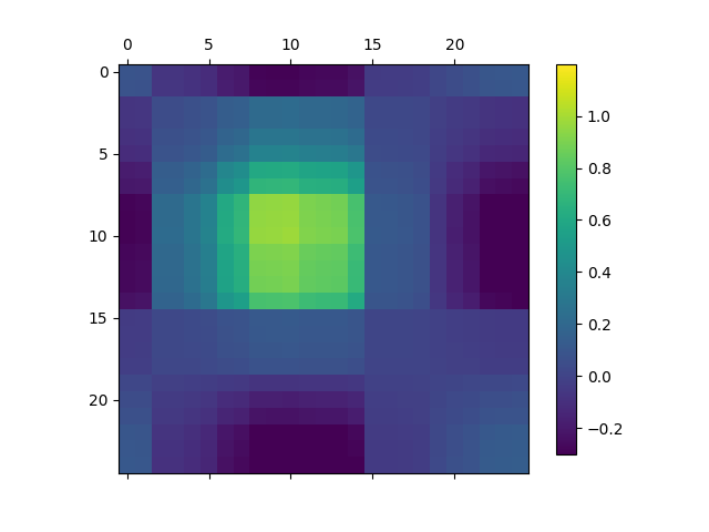
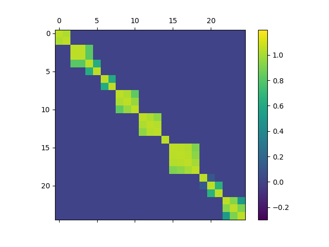
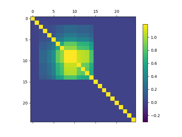
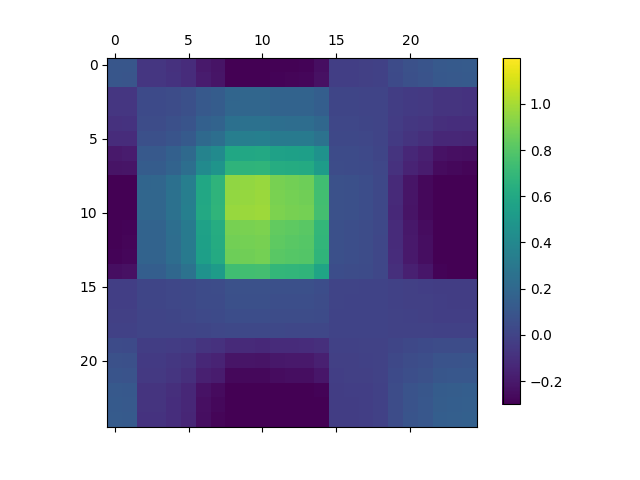
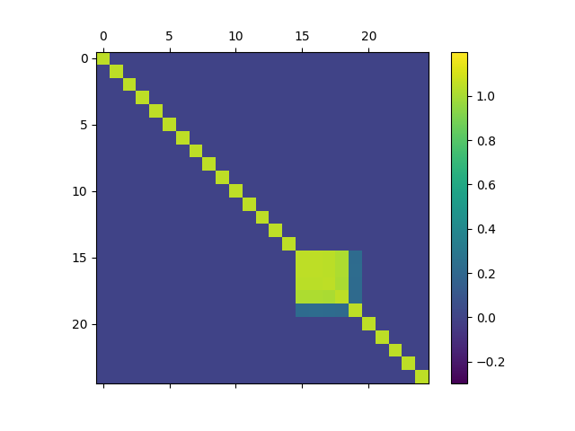
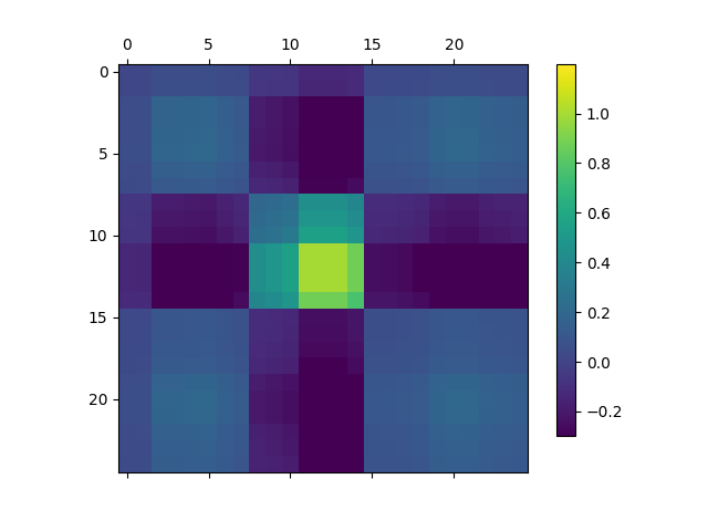
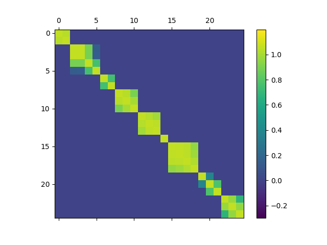
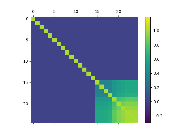
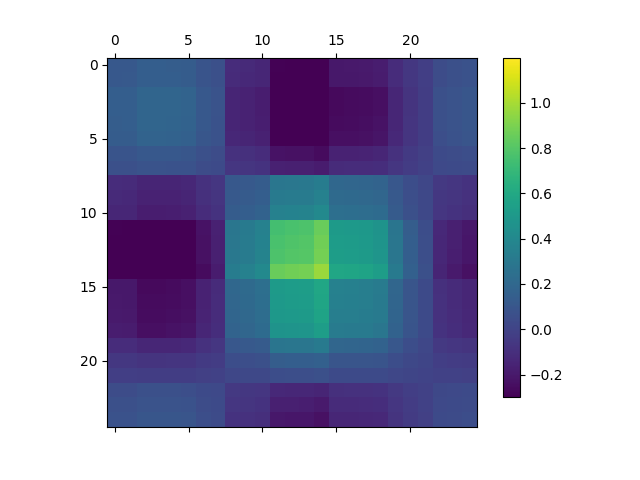
Illustrative examples of $\mathbf{K}_{\mathbf{h}\mathbf{h}}^{r}$ estimated under the different ggp specifications with diagonal posteriors are presented at Figure 5. Heatmaps are shown for different row groups for sites in longitudinal order. As shown for the initial full ggp specification, parameters across row groups were found to be largely consistent with few exceptions (this was also true for latitudinal lengthscales). In contrast, parameters under sparse (explicit) and sparse (implicit) were found to be very adaptive, varying in lengthscale and magnitude. While the explicit sparse construction forces the model to place the most weight on nearest sites, weight centred under the wavelet kernel broadly tended to nearby sites but far less rigidly. Freely parameterized models (not shown) did not tend toward covariance structures estimated for models with explicit kernel definitions. Rather, $\mathbf{K}_{\mathbf{h}\mathbf{h}}^{r}$ in both the full and sparse free models tended to a very sparse diagonal structure.

(a)	(b)	(c)

Figure 5: Examples of $\mathbf{K}_{\mathbf{h}\mathbf{h}}^{r}$ under ggp and sparse ggp model variants for $P=25$ (diagonal). Heatmaps of $\mathbf{K}_{\mathbf{h}\mathbf{h}}^{r}$ are shown for four row-groups in $\mathbf{W}$ for tasks $i=4,10,16,22$ for tasks (sites) ordered by site longitude. Estimated $\mathbf{K}_{\mathbf{h}\mathbf{h}}^{r}$ shown for ggp (Panel (a)), Sparse ggp (explicit) (Panel (b)) and Sparse ggp (implicit) (Panel (c)). Heatmaps in Panel (c) are shown without the diagonal correction term.

References

- [1] Mauricio Álvarez and Neil D Lawrence. Sparse convolved Gaussian processes for multi-output regression. In Neural Information Processing Systems. 2009.
- [2] Mauricio A Álvarez and Neil D Lawrence. Computationally efficient convolved multiple output Gaussian processes. Journal of Machine Learning Research, 12(5):1459–1500, 2011.
- [3] Mauricio A. Álvarez, Lorenzo Rosasco, and Neil D. Lawrence. Kernels for vector-valued functions: A review. Found. Trends Mach. Learn., 4(3):195–266, March 2012.
- [4] J. Antonanzas, N. Osorio, R. Escobar, R. Urraca, F.J. Martinez de Pison, and F. Antonanzas-Torres. Review of photovoltaic power forecasting. Solar Energy, 136:78 – 111, 2016.
- [5] Edwin V Bonilla, Felix V Agakov, and Christopher KI Williams. Kernel multi-task learning using task-specific features. In AISTATS, pages 43–50, 2007.
- [6] Edwin V. Bonilla, Kian Ming A. Chai, and Christopher K. I. Williams. Multi-task Gaussian process prediction. In Neural Information Processing Systems. 2008.
- [7] Noel Cressie and Christopher K Wikle. Statistics for spatio-temporal data. John Wiley & Sons, 2011.
- [8] Kurt Cutajar, Edwin V Bonilla, Pietro Michiardi, and Maurizio Filippone. Random feature expansions for deep gaussian processes. In Proceedings of the 34th International Conference on Machine Learning-Volume 70, pages 884–893. JMLR. org, 2017.
- [9] Kurt Cutajar, Michael Osborne, John Cunningham, and Maurizio Filippone. Preconditioning kernel matrices. In International Conference on Machine Learning, pages 2529–2538, 2016.
- [10] Astrid Dahl and Edwin V Bonilla. Grouped Gaussian processes for solar power prediction. arXiv preprint arXiv:1806.02543, 2018.
- [11] Amir Dezfouli and Edwin V Bonilla. Scalable inference for Gaussian process models with black-box likelihoods. In Neural Information Processing Systems. 2015.
- [12] Trefor Evans and Prasanth Nair. Scalable gaussian processes with grid-structured eigenfunctions (gp-grief). In International Conference on Machine Learning, pages 1416–1425, 2018.
- [13] Jacob Gardner, Geoff Pleiss, Kilian Q Weinberger, David Bindel, and Andrew G Wilson. Gpytorch: Blackbox matrix-matrix gaussian process inference with gpu acceleration. In Advances in Neural Information Processing Systems, pages 7587–7597, 2018.
- [14] Jacob R. Gardner, Geoff Pleiss, Ruihan Wu, Kilian Q. Weinberger, and Andrew Gordon Wilson. Product kernel interpolation for scalable Gaussian processes. arXiv, abs/1802.08903, 2018.
- [15] Marc G Genton. Classes of kernels for machine learning: a statistics perspective. Journal of machine learning research, 2(Dec):299–312, 2001.
- [16] James Hensman, Nicolas Durrande, Arno Solin, et al. Variational fourier features for gaussian processes. Journal of Machine Learning Research, 18:151–1, 2017.
- [17] James Hensman, Nicolo Fusi, and Neil D Lawrence. Gaussian processes for big data. In Uncertainty in Artificial Intelligence, 2013.
- [18] James Hensman, Magnus Rattray, and Neil D. Lawrence. Fast nonparametric clustering of structured time-series. IEEE Transactions on Pattern Analysis and Machine Intelligence, 00 2014.
- [19] Diederik P. Kingma and Jimmy Ba. Adam: A method for stochastic optimization. CoRR, abs/1412.6980, 2014.
- [20] Haitao Liu, Yew-Soon Ong, Xiaobo Shen, and Jianfei Cai. When Gaussian process meets big data: A review of scalable GPs. arXiv preprint arXiv:1807.01065, 2018.
- [21] Joaquin Quinonero-Candela and Carl Edward Rasmussen. Analysis of some methods for reduced rank gaussian process regression. In Switching and learning in feedback systems, pages 98–127. Springer, 2005.
- [22] Joaquin Quiñonero-Candela and Carl Edward Rasmussen. A unifying view of sparse approximate Gaussian process regression. JMLR, 6:1939–1959, 2005.
- [23] J. Quiñonero-Candela, CE. Rasmussen, and CKI. Williams. Approximation Methods for Gaussian Process Regression, pages 203–223. Neural Information Processing. MIT Press, Cambridge, MA, USA, September 2007.
- [24] Carl Edward Rasmussen and Christopher K. I. Williams. Gaussian processes for machine learning. The MIT Press, 2006.
- [25] Håvard Rue, Sara Martino, and Nicolas Chopin. Approximate Bayesian inference for latent Gaussian models by using integrated nested Laplace approximations. Journal of the royal statistical society: Series b (statistical methodology), 71(2):319–392, 2009.
- [26] Ed Snelson and Zoubin Ghahramani. Sparse Gaussian processes using pseudo-inputs. In Neural Information Processing Systems, 2006.
- [27] Arno Solin and Simo Särkkä. Hilbert space methods for reduced-rank gaussian process regression. arXiv preprint arXiv:1401.5508, 2014.
- [28] Dongchu Sun and Xiaoqian Sun. Estimation of the multivariate normal precision and covariance matrices in a star-shape model. Annals of the Institute of Statistical Mathematics, 57(3):455–484, 2005.
- [29] Xiaoqian Sun and Dongchu Sun. Estimation of the cholesky decomposition of the covariance matrix for a conditional independent normal model. Statistics & probability letters, 73(1):1–12, 2005.
- [30] Yee Whye Teh, Matthias Seeger, and Michael I. Jordan. Semiparametric latent factor models. In Artificial Intelligence and Statistics, 2005.
- [31] Michalis Titsias. Variational learning of inducing variables in sparse Gaussian processes. In AISTATS, 2009.
- [32] Cyril Voyant, Gilles Notton, Soteris Kalogirou, Marie-Laure Nivet, Christophe Paoli, Fabrice Motte, and Alexis Fouilloy. Machine learning methods for solar radiation forecasting: A review. Renewable Energy, 105:569 – 582, 2017.
- [33] Ke Alexander Wang, Geoff Pleiss, Jacob R Gardner, Stephen Tyree, Kilian Q Weinberger, and Andrew Gordon Wilson. Exact gaussian processes on a million data points. arXiv preprint arXiv:1903.08114, 2019.
- [34] Joe Whittaker. Graphical models in applied multivariate statistics. Wiley Publishing, 2009.
- [35] Joakim Widen, Nicole Carpman, Valeria Castellucci, David Lingfors, Jon Olauson, Flore Remouit, Mikael Bergkvist, Morten Grabbe, and Rafael Waters. Variability assessment and forecasting of renewables: A review for solar, wind, wave and tidal resources. Renewable and Sustainable Energy Reviews, 44:356–375, 2015.
- [36] Andrew Wilson and Hannes Nickisch. Kernel interpolation for scalable structured gaussian processes (kiss-gp). In International Conference on Machine Learning, pages 1775–1784, 2015.
- [37] Andrew G. Wilson, David A. Knowles, and Zoubin Ghahramani. Gaussian process regression networks. In International Conference on Machine Learning, 2012.
- [38] Dazhi Yang, Jan Kleissl, Christian A Gueymard, Hugo TC Pedro, and Carlos FM Coimbra. History and trends in solar irradiance and pv power forecasting: A preliminary assessment and review using text mining. Solar Energy, 2018.
- [39] Li Zhang, Weida Zhou, and Licheng Jiao. Wavelet support vector machine. IEEE Transactions on Systems, Man, and Cybernetics, Part B (Cybernetics), 34(1):34–39, 2004.