Galerkin Method with Trigonometric Basis on Stable Numerical Differentiation

Abstract

This paper considers the $p$ ($p=1,2,3$) order numerical differentiation on function $y$ in $(0,2\pi)$. They are transformed into corresponding Fredholm integral equation of the first kind. Computational schemes with analytic solution formulas are designed using Galerkin method on trigonometric basis. Convergence and divergence are all analysed in Corollaries 5.1, 5.2, and a-priori error estimate is uniformly obtained in Theorem 6.1, 7.1, 7.2. Therefore, the algorithm achieves the optimal convergence rate $O(\delta^{\frac{2\mu}{2\mu+1}})\ (\mu=\frac{1}{2}\ \textrm{or}\ 1)$ with periodic Sobolev source condition of order $2\mu p$. Besides, we indicate a noise-independent a-priori parameter choice when the function $y$ possesses the form of

$$\sum^{p-1}_{k=0}a_{k}t^{k}+\sum^{N_{1}}_{k=1}b_{k}\cos kt+\sum^{N_{2}}_{k=1}c_{k}\sin kt,\ b_{N_{1}},c_{N_{2}}\neq 0,$$

In particular, in numerical differentiations for functions above, good filtering effect (error approaches 0) is displayed with corresponding parameter choice. In addition, several numerical examples are given to show that even derivatives with discontinuity can be recovered well.

• August 2017

1 Introduction

Numerical differentiation is a classical ill-posed problem which arises in different practical fields, such as option pricing, thermodynamics and photoelectric response (See e.g. [4,11,13-16,25]). In process of numerical differentiation on a given function $y(x)$ of specific smoothness, always there would interfuse with a noise $\delta y$ in measurement or calculations. For this sake, it is routine to do numerical differentiation on the noisy function $y^{\delta}:=y+\delta y$, where the high frequency part in $\delta y$ would bring uncontrolled huge error when computing with traditional numerical algorithms. In order to overcome the difficulties of ill-posedness, several kinds of regularization method were introduced.
Tikhonov method (See [8,11,12,17,26-28]) is a classical regularization method for numerical differentiation of first order. It is generally modeled that, for $x\in[0,1]$ with a grid $\Delta=\{0=x_{0}<x_{1}<\cdots<x_{n}=1\}$ and $h=\max_{i}x_{i+1}-x_{i}$ being its mesh size, given finite noisy samples $\tilde{y}_{i}$ of $y(x_{i})$ such that $|\tilde{y}_{i}-y(x_{i})|\leq\delta$. Assume that $\tilde{y}_{0},\ \tilde{y}_{n}$ are exactly known boundary data, that is, $\tilde{y}_{0}=y(0),\ \tilde{y}_{n}=y(1)$. Then minimizing the cost functional

$$\Psi[f]:=\frac{1}{n-1}\sum^{n-1}_{i=1}(\tilde{y}_{i}-f(x_{i}))^{2}+\alpha\|f^{\prime\prime}\|^{2}$$

in $\{f\in H^{2}(0,1):f(0)=y(0),f(1)=y(0)\}$ gives minimizer $f_{\alpha}$. Afterward differentiating this minimizer gives $f^{\prime}_{\alpha}$ as the regularized solution to the exact derivative $y^{\prime}$ with appropriate parameter choice $\alpha=\alpha(\delta)$. Further results illustrate that $f^{\prime}_{\alpha(\delta)}$ can converge to $y^{\prime}$ with best rate $O(\sqrt{\delta})$ with parameter choice for $\alpha=\delta^{2}$ (See [28]). However, we note that the penalty term $\|f^{\prime\prime}\|$ in cost functional basically demand that the all candidate solutions $f^{\prime}_{\alpha}$ must be at least $H^{1}$ smooth and further result in [27,28] illustrates that, for $y\in C[0,1]/H^{2}(0,1)$, under specific parameter choice $\alpha=\delta^{2}$, the upper bound for $\|f^{\prime}_{\delta^{2}}-y^{\prime}\|$ must tend to infinity as $\delta,h\to 0$. Thus this algorithm naturally deny to recover derivative with regularity less than $H^{1}$, especially discontinuous derivative.
Difference method [4,23] is another classical regularization method for numerical differentiation (including higher orders). It constructs difference quotient of $p$ order as regularized solution to exact derivatives $y^{(p)}$ with the stepsize $h$ being the regularization parameter. The convergence of this scheme is established in $L^{\infty}$ setting and will basically demand that $y^{\prime}\in C^{0,\alpha},\alpha>0$ (See [4]) which also deny to recover derivatives that are only continuous and discontinuous. Furthermore, the best convergence rate $O(\delta^{\frac{2}{3}})$ and $O(\delta^{\frac{1}{3}})$ for first and second order numerical differentiation are derived with $h=O(\delta^{\frac{1}{3}})$ respectively. But we need note the essential flaw in this algorithm that the numerical derivatives constructed by this algorithm will lose its smoothness and all be piecewise constant, whether the original function is smooth or not.
In this paper, we first formulate the $p$ order derivative $y^{(p)}$ as the unique solution of Fredholm integral equation of the first kind

$$A^{(p)}\varphi:=\frac{1}{(p-1)!}\int^{x}_{0}(x-t)^{p-1}\varphi(t)dt=y(x),\ x\in(0,2\pi).$$ (1.1)

where $A^{(p)}:L^{2}(0,2\pi)\to L^{2}(0,2\pi)$. For the simple design of computational scheme, we apply Galerkin method with trigonometric basis to above equation to construct a regularized solutions to $y^{(p)}$ (refer to [9,19-22] for similar techniques). The basic setting can be described as below:
Assume that

$$y^{\delta},\ y,\ \delta y\in L^{2}(0,2\pi)\ \textrm{and}\ \ \|\delta y\|_{L^{2}}\leq\delta,$$

where $\delta$ is noise level. Given a projection sequence $\{P_{n}\}$ which project $L^{2}(0,2\pi)$ onto subspace

$$X_{n}:=span\{\frac{1}{\sqrt{2\pi}},\frac{\cos t}{\sqrt{\pi}},\frac{\sin t}{\sqrt{\pi}},\cdots,\frac{\cos nt}{\sqrt{\pi}},\frac{\sin nt}{\sqrt{\pi}}\},$$

we discrete (1.1) into a finite-rank approximation system

$$A^{(p)}_{n}\varphi_{n}=y_{n}\ \ \varphi_{n}\in X_{n},y_{n}:=P_{n}y\in X_{n},$$ (1.2)

where $A^{(p)}_{n}:=P_{n}A^{(p)}P_{n}:X_{n}\longrightarrow X_{n}$.
Now solving (1.2) in sense of Moore-Penrose inverse gives ${A_{n}^{(p)}}^{\dagger}P_{n}y$. This is a natural approximation scheme for $y^{(p)}$, where $\dagger$ denotes the Moore-Penrose inverse of linear operator. Considering the noise $\delta y$, above scheme should be adjusted to a regularized scheme

$${A_{n}^{(p)}}^{\dagger}P_{n}y^{\delta}\ \textrm{with}\ n^{(p)}=n^{(p)}(\delta),$$ (1.3)

where $n^{(p)}:=n^{(p)}(\delta)$ is the regularization parameter choice such that

$$n^{(p)}:=n^{(p)}(\delta)\to+\infty,\delta\to 0^{+}$$

and

$$\|{A^{(p)}_{n^{(p)}(\delta)}}^{\dagger}P_{n^{(p)}(\delta)}y^{\delta}-y^{(p)}\|_{L^{2}}\to 0,\ \delta\to 0^{+}.$$

Here notice that $n^{(p)}:=n^{(p)}(\delta)\ (p=1,2,3)$ stands for parameter choice strategy of the first three order numerical differentiation respectively. Throughout this paper, without special indication, we follow this notation and $p\in\overline{1,2,3}$.
Main results of this paper and corresponding remarks are listed as follows.

• For $y\in{\mathcal{H}}^{p}_{0}(0,2\pi)$ (this restriction on initial value data is removable), where ${\mathcal{H}}^{p}_{0}(0,2\pi):=\{y\in H^{p}(0,2\pi):y(0)=\cdots=y^{(p-1)}(0)=0\}.$ a priori error estimate is obtained uniformly for first three order numerical differentiation as

  $$\|{A^{(p)}_{n}}^{\dagger}P_{n}y^{\delta}-y^{(p)}\|_{L^{2}(0,2\pi)}\leq C^{(p)}n^{p}\delta+(\gamma^{(p)}+1)\|(I-P_{n})y^{(p)}\|_{L^{2}},$$

  This determines the parameter choice strategy:

  $$n^{(p)}=n^{(p)}(\delta)=\kappa\delta^{a-\frac{1}{p}},$$

  where $a\in(0,\frac{1}{p})$ is optional and $\kappa$ is a constant which depends on the concrete form of $\|(I-P_{n})y^{(p)}\|_{L^{2}}$. This establish a convergence result for numerical differentiation of first three order when $y^{(p)}\in L^{2}$, especially for derivative with discontinuities. However, we need specify that, when recovering $y^{(p)}\in L^{2}$ are only continuous and discontinuous with no periodic smoothness, the constant $\kappa$ is unknown and need to test in experiments (See section 8.3). In addition we give a notice that, whether the derivative is smooth or not, its approximation by above algorithm will be real analytic since it is a trigonometric polynomial.

• Supplemented with a priori information

  $$y^{(p)}\in H_{per}^{l}(0,2\pi),\ l>0\ \ (\textrm{periodic smoothness})$$

  above error estimate is strengthened into a more explicit form as

  $$\|{A^{(p)}_{n}}^{\dagger}P_{n}y^{\delta}-y^{(p)}\|_{L^{2}(0,2\pi)}\leq C^{(p)}n^{p}\delta+(\gamma^{(p)}+1)\frac{1}{n^{l}}\|y^{(p)}\|_{H_{per}^{l}},$$

  where $C^{(p)}$, $\gamma^{(p)}$ are all independent constants given in proceeding sections. And optimal convergence rate $O(\delta^{\frac{2\mu}{2\mu+1}})$ can be derived under periodic Sobolev source condition

  $$y^{(p)}\in H_{per}^{2\mu p}(0,2\pi)\ \ \mu=\frac{1}{2}\ \textrm{or}\ 1,$$

  with parameter choice $n^{(p)}=\lambda^{(p)}\delta^{-\frac{1}{(2\mu+1)p}}$, where $\lambda^{(p)}$ is a constant only depends on exact derivative $y^{(p)}$ and can be given explicitly in preceding sections 6,7. In particular, when

  $$y^{(p)}=a_{0}+\sum^{N_{1}}_{k=1}b_{k}\cos kx+\sum^{N_{2}}_{k=1}c_{k}\sin kx\in H^{\infty}_{per}(0,2\pi)$$

  the optimal parameter choice will degenerate to a constant $n=\max(N_{1},N_{2})$ which does not depend on noise. Furthermore, the numerical study in section 8.1 demonstrates the good filtering effect (error approaches 0) occurs in this specific case.

• In a more general setting for $p$ order numerical differentiation when $y\in H^{p}(0,2\pi)$, it is indicated in Corollary 6.2 that, when $y\in H^{p}(0,2\pi)\setminus{\mathcal{H}}^{p}_{0}(0,2\pi)$,

  $$\|{A^{(p)}_{n}}^{\dagger}P_{n}y\|_{L^{2}}\longrightarrow\infty\ (n\to\infty).$$

  Now any parameter choice $n^{(p)}(\delta)$ such that $n^{(p)}=n^{(p)}(\delta)\to\infty\ (\delta\to 0^{+})$ may not be a proper regularization parameter since we can not determine

  $$\|{A^{(p)}_{n^{(p)}(\delta)}}^{\dagger}P_{n^{(p)}(\delta)}y^{\delta}-y^{(p)}\|_{L^{2}}\to 0,\ \delta\to 0^{+}.$$

  through traditional estimate any more (See second point behind Corollary 5.2). In order to recover the regularization effect of algorithm, we introduce Taylor polynomial truncation of $p-1$ order to reform the regularized scheme, that is, using

  $$\bar{y}=y(x)-\sum^{p-1}_{k=0}\frac{y^{(k)}(0)}{k!}x^{k}\in{\mathcal{H}}^{p}_{0}(0,2\pi),$$

  to replace $y\in H^{p}(0,2\pi)$. In this way, the regularization effect can be well recovered (See section 6,7)with exact measurements on initial value data. Furthermore, we take possible noise in measurements in initial value data into consideration, and this effectively relax the requirement on precision of initial value data.

Outline of Paper: In section 2, we introduce some tools and basic lemmas. In section 3, we illustrate general framework, give the main idea on how to utilize the noisy data $y^{\delta}$ to recover the $p$ order derivatives $y^{(p)}$. In section 4, we give corresponding analytic solution formula to Galerkin approximation system which determines the well-posedness result and upper bound for noise error. In section 5, we propose an estimate on approximation error when RHS $y$ belongs to $\mathcal{H}^{p}_{0}(0,2\pi)$, and give the convergence and divergence results with respect to $y\in\mathcal{H}^{p}_{0}(0,2\pi)$ and $y\in L^{2}(0,2\pi)\setminus\mathcal{H}^{p}_{0}(0,2\pi)$ respectively. In sections 6 and 7, with periodic Sobolev source condition of order $2\mu p$, we construct a priori error estimate and indicate the parameter choice strategy for optimal convergence rate $O(\delta^{\frac{2\mu}{2\mu+1}})$ when $y\in\mathcal{H}^{p}_{0}(0,2\pi)$ and $y\in H^{p}(0,2\pi)\setminus\mathcal{H}^{p}_{0}(0,2\pi)$ respectively. In section 8, we test some numerical examples to show the characteristics and effects of algorithm when derivatives are smooth and discontinuous respectively. In section 9, we conclude the main work of this paper.

2 Preliminary and Basic Lemmas

2.1 Moore-Penrose inverse

Let $X,Y$ be Hilbert space, and $A$ be bounded linear operator mapping from $X$ to $Y$. $\mathcal{D}(A)$, $\mathcal{N}(A)$ and $\mathcal{R}(A)$ denote its domain, null space and range, respectively.
For $A:X\to Y$ and $y\in\mathcal{R}(A)\oplus\mathcal{R}(A)^{\perp}$, the Moore-Penrose inverse $x^{\dagger}:=A^{\dagger}y$ is defined as the element of smallest norm satisfying

$$\|Ax^{\dagger}-y\|=\inf\{\|Ax-y\||x\in X\}.$$

Thus $A^{\dagger}:\mathcal{D}(A^{\dagger}):=\mathcal{R}(A)\oplus\mathcal{R}(A)^{\perp}\subseteq Y\longrightarrow X$ defines a closed linear operator from $Y$ to $X$.
In the following, we indicate some useful properties of Moore-Penrose inverse $A^{\dagger}$:

• If $A:X\to Y$ is one-to-one, then, for $y\in\mathcal{R}(A)$, $A^{\dagger}y$ naturally degenerates into $A^{-1}y$.

• If $\mathcal{R}(A)$ is closed, then $\mathcal{D}(A^{\dagger})=\mathcal{R}(A)\oplus\mathcal{R}(A)^{\perp}=Y$ and by closed graph theorem, $A^{\dagger}:Y\to X$ is bounded.

• If $\mathcal{R}(A)$ is closed, then $AA^{\dagger}=P_{\mathcal{R}(A)},\ A^{\dagger}A=P_{\mathcal{N}(A)^{\perp}}.$ If $\mathcal{R}(A)$ is not necessarily closed, then the former identity need be adjusted into

  $$AA^{\dagger}y=P_{\overline{\mathcal{R}(A)}}y,\ \forall y\in\mathcal{R}(A)\oplus\mathcal{R}(A)^{\perp}.$$ (2.1)

For more comprehensive information on Moore-Penrose inverses, see [2, Chapter 9] or [6,7].

2.2 Sobolev spaces

Throughout this paper, we only discuss on Sobolev space over $\mathrm{R}$. Without specification, we denote $H^{p}(0,2\pi):=H_{\mathrm{R}}^{p}(0,2\pi)$. Here we introduce all kinds of notations of Sobolev spaces which will be used in the context. For more information, see [1,5] and [3, Appendix 4].

2.2.1 Sobolev spaces of integer order

For some positive integer $p$, the Sobolev space $H^{p}(0,2\pi)$ is defined as

$$H^{p}(0,2\pi):=\{y\in L^{2}(0,2\pi):D^{1}y,\cdots,D^{p}y\in L^{2}(0,2\pi)\},$$ (2.2)

where $D^{k}y$ means weak derivative, defined as $\zeta\in L^{2}(0,2\pi)$ which satisfies

$$\int^{2\pi}_{0}\zeta\varphi dx=(-1)^{k}\int^{2\pi}_{0}y\varphi^{(k)}dx,\ \varphi\in C^{\infty}_{0}(0,2\pi).$$

Equivalently, it can be characterized in absolute continuous form (refer to [3, Page 14]) as

$$H^{p}(0,2\pi)=\mathcal{U}^{p}[0,2\pi]:=\{y\in C^{p-1}[0,2\pi]:$$

$$\textrm{there exists}\ \Psi\in L^{2}(0,2\pi)\ \textrm{ such that}\ y^{(p-1)}(x)=\alpha+\int^{x}_{0}\Psi(t)dt,\alpha\in\mathrm{R}\}$$ (2.3)

Here notice that above $"="$ admits a possible change in a set of measure zero. In this paper, when it concerns Sobolev functions of one variable $y\in H^{p}(0,2\pi)$, we, by default, modify $y\in H^{p}(0,2\pi)\ (p\in\mathrm{N})$ in a set of measure zero such that it belongs to the latter fine function space $\mathcal{U}^{p}[0,2\pi]$.
Besides, for $p\in\mathrm{N}$, we define

$${\mathcal{H}}^{p}_{z}(0,2\pi):=\{y\in H^{p}(0,2\pi):y(z)=\cdots=y^{(p-1)}(z)=0\},\ z=0\ \textrm{or}\ 2\pi$$

and

$${\dot{\mathcal{H}}}^{2p}(0,2\pi):=\{y\in H^{2p}(0,2\pi):$$

$$y(2\pi)=\cdots=y^{(p-1)}(2\pi)=y^{(p)}(0)=\cdots=y^{(2p-1)}(0)=0\}.$$

2.2.2 Fractional periodic Sobolev spaces

For real number $s>0$, periodic Sobolev spaces of fractional order $H_{per}^{s}(0,2\pi)$ is defined in trigonometric form as

$$H_{per}^{s}(0,2\pi):=\{\varphi\in L^{2}(0,2\pi):\xi^{2}_{0}+\sum^{\infty}_{k=1}(1+k^{2})^{s}(\xi^{2}_{k}+\eta^{2}_{k})<\infty\},$$

where

$$\xi_{0}=\frac{1}{\sqrt{2\pi}}\int^{2\pi}_{0}\varphi(t)dt,\ \xi_{k}=\frac{1}{\sqrt{\pi}}\int^{2\pi}_{0}\varphi(t)\cos ktdt,\ \eta_{k}=\frac{1}{\sqrt{\pi}}\int^{2\pi}_{0}\varphi(t)\sin ktdt.$$

Supplementing another element $\psi\in H_{per}^{s}(0,2\pi)$, its inner product is rephrased as

$$(\varphi,\psi)_{H_{per}^{s}}=\xi_{0}\zeta_{0}+\sum^{\infty}_{k=1}(1+k^{2})^{s}(\xi_{k}\zeta_{k}+\eta_{k}\lambda_{k})$$

with

$$\zeta_{0}=\frac{1}{\sqrt{2\pi}}\int^{2\pi}_{0}\psi(t)dt,\ \zeta_{k}=\frac{1}{\sqrt{\pi}}\int^{2\pi}_{0}\psi(t)\cos ktdt,\ \lambda_{k}=\frac{1}{\sqrt{\pi}}\int^{2\pi}_{0}\psi(t)\sin ktdt.$$

In addition, we define

$$H^{\infty}_{per}(0,2\pi):=\bigcap_{s>0}H^{s}_{per}(0,2\pi).$$

2.3 Integro-differential operator of $p$ order

Define integro-differential operator of integer order $p$ as:

$$A^{(p)}:L^{2}(0,2\pi)\longrightarrow L^{2}(0,2\pi)$$

$$\varphi\longmapsto(A^{(p)}\varphi)(x):=\frac{1}{\Gamma(p)}\int^{x}_{0}(x-t)^{p-1}\varphi(t)dt,\ x\in(0,2\pi).$$ (2.4)

This is a compact linear operator with infinite-dimensional range, which satisfies

Lemma 2.1

$${\mathcal{H}}^{p}_{0}(0,2\pi)=\mathcal{R}(A^{(p)}),\ p=1,2,3.$$

Proof 1

”$\subseteq$”: Assume that $y\in{\mathcal{H}}^{p}_{0}(0,2\pi)\ (p=1,2,3)$. There exists a $y^{\star}\in\mathcal{U}^{p}[0,2\pi]$ as a modification of $y$ in a possible $0$ measure set with $0$ initial value data, that is, $y^{\star}(0)=\cdots={y^{\star}}^{(p-1)}(0)=0$. With integration formula by parts, it is not difficult to verify that,

$$\frac{1}{(p-1)!}\int^{x}_{0}(x-t)^{p-1}{y^{\star}}^{(p)}(t)dt=y^{\star}(x)=y(x),\ a.e..$$

Thus,

$${\mathcal{H}}^{p}_{0}(0,2\pi)\subseteq\mathcal{R}(A^{(p)}),\ p=1,2,3.$$

”$\supseteq$”: For simplicity, we only provide proof of case $p=2$. Assuming $y\in\mathcal{R}(A^{(2)})$, then there exists a $\varphi\in L^{2}(0,2\pi)$ such that

$$\int^{x}_{0}(x-t)\varphi(t)dt=y(x),\ a.e..$$

It is not difficult to verify that

$$D^{1}y=\int^{x}_{0}\varphi(t)dt,\ D^{2}y=\varphi(t)\ a.e.$$

With definition of (2.2), it yields that $y\in H^{2}(0,2\pi)$. Then by absolute continuous characterization (2.3) of Sobolev function of one variable, there exist a $y^{\star}\in\mathcal{U}^{2}[0,2\pi]$ as modification of $y$ in a $0$ measure set. Thus we have

$$y^{\star}=\int^{x}_{0}(x-t)\varphi(t)dt,\ {y^{\star}}^{\prime}=D^{1}y^{\star}=D^{1}y=\int^{x}_{0}\varphi(t)dt,\ a.e.$$

Notice that

$$y^{\star},\ {y^{\star}}^{\prime},\ \int^{x}_{0}(x-t)\varphi(t)dt,\ \int^{x}_{0}\varphi(t)dt$$

are all continuous functions, thus

$$y^{\star}=\int^{x}_{0}(x-t)\varphi(t)dt,\ {y^{\star}}^{\prime}=\int^{x}_{0}\varphi(t)dt.\ (\textrm{strictly})$$

”$\supseteq$” holds for case $p=2$.

With above equality, we describe the density of range in $L^{2}(0,2\pi)$.

Lemma 2.2

$$\overline{\mathcal{R}(A^{(p)})}=L^{2}(0,2\pi),\ P_{\overline{\mathcal{R}(A^{(p)})}}=I\ \ (p=1,2,3),$$

where $I$ is the identity operator on $L^{2}(0,2\pi)$.

Proof 2

With Lemma 2.1, ${\mathcal{H}}^{p}_{0}(0,2\pi)=\mathcal{R}(A^{(p)}).$ Recall the fact that $C^{\infty}_{0}(0,2\pi)$ is dense in $L^{2}(0,2\pi)$ and notice that $C^{\infty}_{0}(0,2\pi)\subseteq{\mathcal{H}}^{p}_{0}(0,2\pi)$, then $L^{2}(0,2\pi)=\overline{C^{\infty}_{0}(0,2\pi)}\subseteq\overline{{\mathcal{H}}^{p}_{0}(0,2\pi)}\subseteq L^{2}(0,2\pi).$ The result follows.

This implies that $\mathcal{R}(A^{(p)})^{\perp}={0}$, and

$$\mathcal{D}({A^{(p)}}^{\dagger})=\mathcal{R}(A^{(p)})\oplus\mathcal{R}(A^{(p)})^{\perp}=\mathcal{R}(A^{(p)})={\mathcal{H}}^{p}_{0}(0,2\pi).$$

Now differentiating the both sides of equation (1.1) for $y\in\mathcal{H}^{p}_{0}(0,2\pi)$ in $p$ order yields that ${A^{(p)}}^{\dagger}y={A^{(p)}}^{-1}y=y^{(p)}$. This gives

Lemma 2.3

${A^{(p)}}^{\dagger}y=y^{(p)},\ \forall y\in{\mathcal{H}}^{p}_{0}(0,2\pi).$

2.4 Galerkin Projection scheme with Moore-Penrose inverses

Let $X$ be Hilbert space. For the linear operator equation

$$A\varphi=y,$$

where $A:X\longrightarrow X$ is bounded and linear. To approximate

$$\varphi^{\dagger}:=A^{\dagger}y\in X,$$

We introduce a sequence of finite-dimensional subspaces $\{X_{n}\}$, which satisfies

$$X_{n}\subseteq X_{n+1},\ \overline{\bigcup^{\infty}_{n=1}X_{n}}=X.$$

Then construct a sequence of orthogonal projections $\{P_{n}\}$, where $P_{n}$ projects $X$ onto $X_{n}$, and gives Galerkin approximation setting

$$A_{n}\varphi_{n}=y_{n},\ \ y_{n}:=P_{n}y\in X_{n},$$ (2.5)

where $A_{n}:=P_{n}AP_{n}:X_{n}\longrightarrow X_{n}$. Hence solving (2.5) in sense of Moore-Penrose inverse gives Galerkin projection scheme

$$\varphi^{\dagger}_{n}:=A^{\dagger}_{n}y_{n}\in X_{n},$$ (2.6)

where $A^{\dagger}_{n}:\mathcal{R}(A_{n})+{\mathcal{R}(A_{n})}^{\perp_{n}}=X_{n}\longrightarrow X_{n}$. Notice that $\perp_{n}$ means orthogonal complement in finite dimensional Hilbert space $X_{n}$.
Now $\{\varphi^{\dagger}_{n}\}$ is a natural approximate scheme for $\varphi^{\dagger}$. To study its convergence property, we introduce the Groetsch regularizer for setting (2.5) as

$$R_{n}:=A_{n}^{\dagger}P_{n}A:X\longrightarrow X_{n}\subseteq X,$$

define the Groetsch regularity as $\ \sup\limits_{n}\|R_{n}\|<+\infty$, and introduce the following result:

Lemma 2.4

For above Galerkin approximate setting (2.5), if Groetsch regularity holds, then
(a) For $y\in\mathcal{D}(A^{\dagger})=\mathcal{R}(A)+\mathcal{R}(A)^{\perp}$.

$$\|A^{\dagger}_{n}P_{n}P_{\overline{\mathcal{R}(A)}}y-A^{\dagger}y\|\leq\|P_{\mathcal{N}(A_{n})}A^{\dagger}y\|+\|R_{n}-I_{X}\|\|(I-P_{n})A^{\dagger}y\|,$$ (2.7)

(b) For $y\notin\mathcal{D}(A^{\dagger})$,

$$\lim_{n\to\infty}\|A^{\dagger}_{n}P_{n}P_{\overline{\mathcal{R}(A)}}y\|=\infty.$$

Proof 3

see[18, theorem 2.2]

2.5 Higher order estimate under trigonometric basis

To further estimate the right term $\|(I-P_{n})A^{\dagger}y\|$ under trigonometric basis in $L^{2}$, similar to the result [3, Lemma A.43], we introduce another error estimate:

Lemma 2.5

Let $P_{n}:L^{2}(0,2\pi)\longrightarrow X_{n}\subset L^{2}(0,2\pi)$ be an orthogonal projection operator, where

$$X_{n}:=\{\xi_{0}\cdot\frac{1}{\sqrt{2\pi}}+\sum\limits^{n}_{k=1}\xi_{k}\frac{\cos kt}{\sqrt{\pi}}+\sum\limits^{n}_{k=1}\eta_{k}\frac{\sin kt}{\sqrt{\pi}}:\ \xi_{0},\xi_{k},\eta_{k}\in\mathrm{R}\}.$$

Then $P_{n}$ is given as follows

$$(P_{n}x)(t)=\xi_{0}\frac{1}{\sqrt{2\pi}}+\sum\limits^{n}_{k=1}\xi_{k}\frac{\cos kt}{\sqrt{\pi}}+\sum^{n}_{k=1}\eta_{k}\frac{\sin kt}{\sqrt{\pi}},$$

where

$$\xi_{0}=\frac{1}{\sqrt{2\pi}}\int^{2\pi}_{0}x(t)dt,\ \xi_{k}=\int^{2\pi}_{0}x(t)\frac{\cos kt}{\sqrt{\pi}}dt,$$

$$\eta_{k}=\int^{2\pi}_{0}x(t)\frac{\sin kt}{\sqrt{\pi}}dt,\ \ 1\leq k\leq n$$

are the Fourier coefficients of $x$. Furthermore, the following estimate holds:

$$\|x-P_{n}x\|_{L^{2}}\leq\frac{1}{n^{r}}\|x\|_{H_{per}^{r}}\ \ for\ all\ x\in\ H_{per}^{r}(0,2\pi),$$

where $r\geq 0$.

3 General Framework

We start from

Problem 3.1

Assume that we have $y\in{\mathcal{H}}^{p}_{0}(0,2\pi)$ and $y^{\delta}$ measured on $(0,2\pi)$, belonging to $L^{2}(0,2\pi)$ such that $\|y^{\delta}-y\|_{L^{2}}\leq\delta$. How to get a stable approximation to $y^{(p)}$ ?

In Lemma 2.3, we have known that $y^{(p)}$ is the solution of linear operator equation

$$A^{(p)}\varphi:=\frac{1}{\Gamma(p)}\int^{x}_{0}(x-t)^{p-1}\varphi(t)dt=y(x),\ x\in(0,2\pi),$$ (3.1)

when

$$y\in{\mathcal{H}}^{p}_{0}(0,2\pi):=\{y\in H^{p}(0,2\pi):y(0)=\cdots=y^{(p-1)}(0)=0\}.$$

3.1 Formulation of finite-dimensional approximation system

In the following, we consider to approximate $y^{(p)}$ by the Galerkin method. Set

$$A^{(p)}:X=L^{2}(0,2\pi)\longrightarrow L^{2}(0,2\pi).$$

Choose a sequence of orthogonal projection operators $\{P_{n}\}$, where $P_{n}$ projects $L^{2}(0,2\pi)$ onto

$$X_{n}:=span\{\frac{1}{\sqrt{2\pi}},\frac{\cos t}{\sqrt{\pi}},\frac{\sin t}{\sqrt{\pi}},\cdots,\frac{\cos nt}{\sqrt{\pi}},\frac{\sin nt}{\sqrt{\pi}}\}.$$

Then degenerate the original operator equation with noisy data

$$A^{(p)}\varphi=y^{\delta}$$

into a finite-rank system

$$A_{n}^{(p)}\varphi_{n}=y^{\delta}_{n},$$ (3.2)

where

$$A_{n}^{(p)}:=P_{n}A^{(p)}P_{n}:X_{n}\longrightarrow X_{n},\ \ y^{\delta}_{n}:=P_{n}y^{\delta}.$$ (3.3)

Span $A_{n}^{(p)}$ under above basis, then the finite-rank system (3.2) is transformed into the linear system as

$$M_{n}^{(p)}u_{n}=b^{\delta}_{n},\ u_{n},b^{\delta}_{n}\in\mathrm{R}^{2n+1}.$$ (3.4)

Notice that $M_{n}^{(p)}$ and $b^{\delta}_{n}$ are defined as follows:

$$M_{n}^{(p)}:=(m_{ij}^{(p)})_{(2n+1)\times(2n+1)}$$

where

$$m_{ij}^{(p)}:=(A^{(p)}_{n}(\xi_{j}),\xi_{i})_{L^{2}},\ i,j\in\overline{0,1,2,\cdots,2n-1,2n}$$

$$\xi_{0}:=\frac{1}{\sqrt{2\pi}},\xi_{2k-1}:=\frac{\cos kx}{\sqrt{\pi}},\xi_{2k}:=\frac{\sin kx}{\sqrt{\pi}},\ k\in\overline{1,2,\cdots,n}.$$

Indeed,

$$A_{n}^{(p)}(\frac{1}{\sqrt{2\pi}},\frac{\cos t}{\sqrt{\pi}},\frac{\sin t}{\sqrt{\pi}},\cdots,\frac{\cos nt}{\sqrt{\pi}},\frac{\sin nt}{\sqrt{\pi}})$$

$$=(\frac{1}{\sqrt{2\pi}},\frac{\cos t}{\sqrt{\pi}},\frac{\sin t}{\sqrt{\pi}},\cdots,\frac{\cos nt}{\sqrt{\pi}},\frac{\sin nt}{\sqrt{\pi}})M_{n}^{(p)}.$$ (3.5)

And $b^{\delta}_{n}:=(f_{0},f_{1},g_{1},\cdots,f_{n},g_{n})^{T}$ is defined as

$$f_{0}:=\int^{2\pi}_{0}y^{\delta}(t)\frac{1}{\sqrt{2\pi}}dt$$

$$f_{k}:=\int^{2\pi}_{0}y^{\delta}(t)\frac{\cos kt}{\sqrt{\pi}}dt,\ g_{k}:=\int^{2\pi}_{0}y^{\delta}(t)\frac{\sin kt}{\sqrt{\pi}}dt,k\in\overline{1,2,\cdots,n}.$$

Indeed,

$$y^{\delta}_{n}=(\frac{1}{\sqrt{2\pi}},\frac{\cos t}{\sqrt{\pi}},\frac{\sin t}{\sqrt{\pi}},\cdots,\frac{\cos nt}{\sqrt{\pi}},\frac{\sin nt}{\sqrt{\pi}})b_{n}^{\delta}.$$

Once we figure out ${u_{n}^{p,\delta}}={M_{n}^{(p)}}^{\dagger}b^{\delta}_{n}$, then we obtain solution for (3.2),

$${\varphi_{n}^{p,\delta}}=(\frac{1}{\sqrt{2\pi}},\frac{\cos t}{\sqrt{\pi}},\frac{\sin t}{\sqrt{\pi}},\cdots,\frac{\cos nt}{\sqrt{\pi}},\frac{\sin nt}{\sqrt{\pi}}){u^{p,\delta}_{n}}.$$

in sense of Moore-Penrose inverse, ${\varphi_{n}^{p,\delta}}={A_{n}^{(p)}}^{\dagger}y^{\delta}_{n}$. This is the regularized scheme. In the following, we need to determine a regularization parameter $n^{(p)}=n^{(p)}(\delta)$ such that

$${\varphi_{n^{(p)}(\delta)}^{p,\delta}}:={A_{n^{(p)}(\delta)}^{(p)}}^{\dagger}y^{\delta}_{n^{(p)}(\delta)}\stackrel{{\scriptstyle s}}{{\longrightarrow}}y^{(p)},\ \delta\to 0^{+}.$$

3.2 Total error estimate and parameter choice for regularization

Now, in order to control the accuracy of computation, we adjust parameter choice strategy $n^{(p)}=n^{(p)}(\delta)$ according to following total error estimate

$$\|\varphi^{p,\delta}_{n}-y^{(p)}\|_{L^{2}}:=\|{A^{(p)}_{n}}^{\dagger}P_{n}y^{\delta}-y^{(p)}\|_{L^{2}}.$$ (3.6)

Since Lemma 2.3 illustrates that

$$y^{(p)}={A^{(p)}}^{\dagger}y,\ y\in{\mathcal{H}}^{p}_{0}(0,2\pi),$$ (3.7)

inserting (3.7) into (3.6), the formula (3.6) becomes

$$\|{A^{(p)}_{n}}^{\dagger}P_{n}y^{\delta}-{A^{(p)}}^{\dagger}y\|_{L^{2}},\ y\in{\mathcal{H}}^{p}_{0}(0,2\pi).$$

Throughout this paper we use the following definitions

• Total error

  $$e^{(p)}_{T}:=\|{A^{(p)}_{n}}^{\dagger}P_{n}y^{\delta}-{A^{(p)}}^{\dagger}y\|_{L^{2}},$$

which is broken into two parts (c.f.[10, Chapter 1.1]):

• Noise error:

  $$e^{(p)}_{N}:=\|{A^{(p)}_{n}}^{\dagger}P_{n}y^{\delta}-{A^{(p)}_{n}}^{\dagger}P_{n}y\|_{L^{2}}$$

• Approximation error:

  $$e^{(p)}_{A}:=\|{A^{(p)}_{n}}^{\dagger}P_{n}y-{A^{(p)}}^{\dagger}y\|_{L^{2}}$$

It is an easy observation that $e^{(p)}_{T}\leq e^{(p)}_{N}+e^{(p)}_{A}$. Upon this fact, we figure out the total error estimate by estimating $e^{(p)}_{N}$ and $e^{(p)}_{A}$ respectively.

4 Well-posedness and numerical scheme of Galerkin System

With concrete expressions of $M^{(p)}_{n}$ in Appendix A, it is not difficult to obtain:

Theorem 4.1

Finite dimensional system (3.4) is well-posed, that is, there exists a unique solution to (3.4), denoted as

$$u^{p,\delta}_{n}={M^{(p)}_{n}}^{-1}b^{\delta}_{n},$$

where

$$b^{\delta}_{n}=(f_{0},f_{1},g_{1},\cdots,f_{n},g_{n})^{T},u^{p,\delta}_{n}=(\xi^{(p)}_{0},\xi^{(p)}_{1},\eta^{(p)}_{1},\cdots,\xi^{(p)}_{n},\eta^{(p)}_{n})^{T}.$$

Moreover, analytic formulas for the solution of Galerkin approximation system (3.2) are determined as follows:

$${A^{(p)}_{n}}^{\dagger}P_{n}y=\xi^{(p)}_{0}\frac{1}{\sqrt{2\pi}}+\sum^{n}_{k=1}\xi^{(p)}_{k}\frac{\cos kt}{\sqrt{\pi}}+\sum^{n}_{k=1}\eta^{(p)}_{k}\frac{\sin kt}{\sqrt{\pi}}.$$

Corresponding three cases are listed as follows.
Case $p=1$:

$$\xi^{(1)}_{0}=\frac{1}{\pi}(f_{0}+\sqrt{2}\sum_{k=1}^{n}f_{k}),$$ (4.1)

$$\xi^{(1)}_{k}=\sqrt{2}\xi^{(1)}_{0}+kg_{k},$$ (4.2)

$$\eta^{(1)}_{k}=-kf_{k}.$$ (4.3)

Case $p=2$:

$$\xi^{(2)}_{0}=\frac{L^{-1}_{n}}{4\pi^{2}}(f_{0}+\sqrt{2}\sum_{k=1}^{n}f_{k}+\frac{\sqrt{2}\pi}{2n+1}\sum_{k=1}^{n}kg_{k}),$$ (4.4)

$$\xi^{(2)}_{k}=\sqrt{2}\xi^{(2)}_{0}-k^{2}f_{k},$$ (4.5)

$$\eta^{(2)}_{k}=\frac{2k}{2n+1}\sum^{n}_{k=1}kg_{k}-k^{2}g_{k}-\frac{\sqrt{2}k\pi}{2n+1}\xi^{(2)}_{0},$$ (4.6)

where

$$L_{n}:=\frac{1}{6}+\frac{1}{2\pi^{2}}S_{n}-\frac{1}{4}\frac{2n}{2n+1},\ S_{n}:=\sum^{n}_{k=1}\frac{1}{k^{2}}.$$

Case $p=3$:

$$\xi^{(3)}_{0}=\frac{T^{-1}_{n}}{4\pi^{3}}(f_{0}+\sqrt{2}\sum\limits_{k=1}^{n}f_{k}+\frac{\sqrt{2}\pi}{2n+1}\sum\limits_{k=1}^{n}kg_{k}-F_{n}\sum\limits_{k=1}^{n}k^{2}f_{k}),$$ (4.7)

$$\xi^{(3)}_{k}=-k^{3}g_{k}+\frac{2}{2n+1}k^{2}\sum\limits_{k=1}^{n}kg_{k}-\frac{2\pi k^{2}}{(2n+1)^{2}}\sum^{n}_{k=1}k^{2}f_{k}+\varepsilon_{n,k}\xi^{(3)}_{0}$$ (4.8)

$$\eta^{(3)}_{k}=k^{3}f_{k}-\frac{2k}{2n+1}\sum\limits_{k=1}^{n}k^{2}f_{k}-\frac{\sqrt{2}\pi k}{2n+1}\xi^{(3)}_{0},$$ (4.9)

where

$$T_{n}:=\frac{1}{12}+\frac{1}{2n+1}\frac{1}{\pi^{2}}S_{n}-\frac{1}{3}\frac{2n}{2n+1}+\frac{n^{2}}{(2n+1)^{2}},$$

$$F_{n}:=\frac{4\sqrt{2}\pi^{2}}{2n+1}L_{n},\ K_{n}:=-2\pi^{2}L_{n},\varepsilon_{n,k}=\sqrt{2}(1+\frac{2k^{2}}{2n+1}K_{n}).$$

Remark 4.1

After we solve the Galerkin approximation system, we know that $A^{(p)}_{n}:X_{n}\to X_{n}$ is one-to-one and surjective. For the usage of the proceeding section, we claim that $\mathcal{N}(A^{(p)}_{n})=0,\ \mathcal{R}(A^{(p)})=X_{n}.$

Remark 4.2

With above analytic formulas, it is not difficult to figure out that

$$\|{A_{n}^{(p)}}^{\dagger}\|_{X_{n}\to X_{n}}\leq C^{(p)}n^{p}$$ (4.10)

where $C^{(1)}=\sqrt{3},\ C^{(2)}\approx 11.8040,\ C^{(3)}\approx 345.0754$. Here we specify that $\|\cdot\|_{X_{n}}$ is induced by $\|\cdot\|_{L^{2}}$, that is, $\|x_{n}\|_{X_{n}}:=\|x_{n}\|_{L^{2}}$, $\forall x_{n}\in X_{n}$. This give bound to the estimate of noise error.

5 Estimate on Approximation Error and Instability result

We use Lemma 2.4 to analyse the convergence and divergence of Galerkin method. The key point is the estimate of

$$\sup_{n}\|R^{(p)}_{n}\|<+\infty,\textrm{where}\ R^{(p)}_{n}:={A^{(p)}_{n}}^{\dagger}P_{n}A^{(p)}.$$ (5.1)

To gain an uniform upper bound for above formula, we first prepare two decay estimate of

$$R^{(p)}_{n}(\frac{\cos jt}{\sqrt{\pi}})\ \textrm{and}\ R^{(p)}_{n}(\frac{\sin jt}{\sqrt{\pi}})$$

with respect to integer variable $j$:

Lemma 5.1

For operators $A^{(p)},A^{(p)}_{n}$ defined in (2.4),(3.3) respectively, set

$$({A^{(p)}_{n}}^{\dagger}P_{n}A^{(p)}(\frac{\cos jt}{\sqrt{\pi}})(t)=\alpha^{(p)}_{0}\frac{1}{\sqrt{2\pi}}+\sum^{n}_{k=1}\alpha^{(p)}_{k}\frac{\cos kt}{\sqrt{\pi}}+\sum^{n}_{k=1}\beta^{(p)}_{k}\frac{\sin kt}{\sqrt{\pi}}.$$

When $j\geq n+1$,

$$\alpha^{(p)}_{0}=\alpha^{(p)}_{0}(n,j)=(({A^{(p)}_{n}}^{\dagger}P_{n}A^{(p)}(\frac{\cos jt}{\sqrt{\pi}}),\frac{1}{\sqrt{2\pi}})_{L^{2}},$$

$$\alpha^{(p)}_{k}=\alpha^{(p)}_{k}(n,j)=(({A^{(p)}_{n}}^{\dagger}P_{n}A^{(p)}(\frac{\cos jt}{\sqrt{\pi}}),\frac{\cos kt}{\sqrt{\pi}})_{L^{2}},$$

$$\beta^{(p)}_{k}=\beta^{(p)}_{k}(n,j)=(({A^{(p)}_{n}}^{\dagger}P_{n}A^{(p)}(\frac{\cos jt}{\sqrt{\pi}}),\frac{\sin kt}{\sqrt{\pi}})_{L^{2}},$$

and

$$|\alpha^{(p)}_{0}|\leq\frac{C_{1}^{(p)}}{j},\ |\alpha^{(p)}_{k}|\leq\frac{C_{2}^{(p)}}{j},|\beta^{(p)}_{k}|\leq\frac{C_{3}^{(p)}}{j},\ 1\leq k\leq n.$$ (5.2)

where

$$C_{1}^{(1)}=0,\ C_{1}^{(2)}=\sqrt{2},\ C_{1}^{(3)}=11\sqrt{2},$$

$$C_{2}^{(1)}=0,\ C_{2}^{(2)}=2,\ C_{2}^{(3)}=23,$$

$$C_{3}^{(1)}=0,\ C_{3}^{(2)}=\pi,\ C_{3}^{(3)}=11\pi.$$

When $p=3$, we need an extra condition $n\geq 5$ to maintain above estimate.

Proof 4

Case $p=1$: When $j\geq n+1$, substituting (B.1) into (4.1),(4.2) and (4.3), it follows that

$$({A^{(1)}_{n}}^{\dagger}P_{n}A^{(1)}(\frac{\cos jt}{\sqrt{\pi}}))(t)={A^{(1)}_{n}}^{\dagger}(0)=0.$$

This gives lemma for case $p=1$.
Case $p=2$: Inserting (B.2) into (4.4), it follows that

$$\alpha^{(2)}_{0}=\frac{\sqrt{2}L^{-1}_{n}}{4\pi^{2}j^{2}}.$$

Hence

$$0\leq\alpha^{(2)}_{0}\leq\frac{\sqrt{2}}{j}\ (\textrm{by (C.1)}).$$ (5.3)

Besides, inserting (B.2) into (4.5),(4.6) respectively, it yields that

$$\alpha^{(2)}_{k}=\sqrt{2}\alpha^{(2)}_{0},\beta^{(2)}_{k}=-\frac{\sqrt{2}k\pi}{2n+1}\alpha^{(2)}_{0}.$$

Then, by (5.3),

$$0\leq\alpha^{(2)}_{k}\leq\frac{2}{j},\ -\frac{\pi}{j}\leq\beta^{(2)}_{k}\leq 0.$$

Case $p=3$: Inserting (B.3) into (4.7), it follows that

$$\alpha^{(3)}_{0}=\frac{T^{-1}_{n}}{4\pi^{3}}\frac{\sqrt{2}\pi}{j^{2}}\frac{1}{2n+1}.$$

Notice Proposition C.1 (C.4),

$$T_{n}\in[\frac{1}{396}\frac{1}{n}\frac{1}{2n+1},\frac{3}{40}\frac{1}{n(2n+1)}],\ n\geq 5.$$

Hence,

$$0\leq\alpha^{(3)}_{0}\leq\frac{11\sqrt{2}}{j},\ \textrm{where}\ \alpha^{(3)}_{0}:=\alpha^{(3)}_{0}(n,j),\textrm{and}\ n\geq 5.$$ (5.4)

Besides, insert (B.3) into (4.8), then it follows that

$$\alpha^{(3)}_{k}=\frac{1}{2n+1}\frac{2k^{2}}{j^{2}}+\sqrt{2}(1+\frac{2k^{2}}{2n+1}K_{n})\alpha^{(3)}_{0}.$$ (5.5)

By Proposition C.1(C.2), it is routine to obtain that

$$\frac{2k^{2}}{2n+1}K_{n}\in[-2,0],\ 1+\frac{2k^{2}}{2n+1}K_{n}\in[-1,1].$$

Hence, with (5.4),

$$0\leq|\alpha^{(3)}_{k}|\leq\frac{23}{j}.$$

Further, insert (B.3) into (4.9), and we have

$$\beta^{(3)}_{k}=-\frac{\sqrt{2}\pi k}{2n+1}\alpha^{(3)}_{0}.$$

Hence

$$-\frac{11\pi}{j}\leq\beta^{(3)}_{k}\leq 0\ \ (\textrm{by (5.4)}).$$

Lemma 5.2

For operators $A^{(p)},A^{(p)}_{n}$ defined in (2.4),(3.3) respectively, set

$$({A^{(p)}_{n}}^{\dagger}P_{n}A^{(p)}(\frac{\sin jt}{\sqrt{\pi}})(t)=\theta^{(p)}_{0}\frac{1}{\sqrt{2\pi}}+\sum^{n}_{k=1}\theta^{(p)}_{k}\frac{\cos kt}{\sqrt{\pi}}+\sum^{n}_{k=1}\omega^{(p)}_{k}\frac{\sin kt}{\sqrt{\pi}}.$$

When $j\geq n+1$,

$$\theta^{(p)}_{0}=\theta^{(p)}_{0}(n,j)=(({A^{(p)}_{n}}^{\dagger}P_{n}A^{(p)}(\frac{\sin jt}{\sqrt{\pi}}),\frac{1}{\sqrt{2\pi}})_{L^{2}},$$

$$\theta^{(p)}_{k}=\theta^{(p)}_{k}(n,j)=(({A^{(p)}_{n}}^{\dagger}P_{n}A^{(p)}(\frac{\sin jt}{\sqrt{\pi}}),\frac{\cos kt}{\sqrt{\pi}})_{L^{2}},$$

$$\omega^{(p)}_{k}=\omega^{(p)}_{k}(n,j)=(({A^{(p)}_{n}}^{\dagger}P_{n}A^{(p)}(\frac{\sin jt}{\sqrt{\pi}}),\frac{\sin kt}{\sqrt{\pi}})_{L^{2}},$$

and

$$|\theta^{(p)}_{0}|\leq\frac{C_{4}^{(p)}}{j},\ |\theta^{(p)}_{k}|\leq\frac{C_{5}^{(p)}}{j},|\omega^{(p)}_{k}|\leq\frac{C_{6}^{(p)}}{j},\ 1\leq k\leq n.$$ (5.6)

where

$$C_{4}^{(1)}=\frac{\sqrt{2}}{\pi},\ C_{4}^{(2)}=\frac{3\sqrt{2}}{2},\ C_{4}^{(3)}=\frac{44\sqrt{2}}{3},$$

$$C_{5}^{(1)}=\frac{2}{\pi},\ C_{5}^{(2)}=3,\ C_{5}^{(3)}=30,$$

$$C_{6}^{(1)}=0,\ C_{6}^{(2)}=5,\ C_{6}^{(3)}=48.$$

Notice that when $p=3$, we need the extra condition $n\geq 5$ to maintain above estimate.

Proof 5

Case $p=1$: When $j\geq n+1$, insert (B.4) into (4.1),(4.2),(4.3), then

$$({A^{(1)}_{n}}^{\dagger}P_{n}A^{(1)}(\frac{\sin jt}{\sqrt{\pi}}))(t)={A^{(1)}_{n}}^{\dagger}(\frac{\sqrt{2}}{j}\cdot\frac{1}{\sqrt{2\pi}})=\frac{\sqrt{2}}{\pi j}\cdot\frac{1}{\sqrt{2\pi}}+\sum^{n}_{k=1}\frac{2}{\pi j}\cdot\frac{\cos kt}{\sqrt{\pi}}.$$

This gives lemma for case $p=1$.
Case $p=2$: Insert (B.5) into (4.4), and it follows that

$$\theta^{(2)}_{0}=\frac{1}{2n+1}\frac{\sqrt{2}}{4\pi j}L^{-1}_{n}.$$

With Proposition C.1 (C.1), it follows that

$$0\leq\theta^{(2)}_{0}\leq\frac{3\sqrt{2}}{2j}.$$ (5.7)

Besides, insert (B.5) into (4.5),(4.6), then

$$\theta^{(2)}_{k}=\sqrt{2}\theta^{(2)}_{0},\ \omega^{(2)}_{k}=\frac{1}{j}\frac{2k}{2n+1}-\frac{k}{2n+1}\cdot\sqrt{2}\pi\theta^{(2)}_{0}.$$

Then by (5.7) we have

$$0\leq\theta^{(2)}_{k}\leq\frac{3}{j},\ -\frac{5}{j}\leq\omega^{(2)}_{k}\leq\frac{1}{j}.$$

Case $p=3$: Insert (B.6) into (4.7), and it follows that

$$\theta^{(3)}_{0}=\frac{T^{-1}_{n}}{4\pi^{3}}\frac{1}{j}(F_{n}-\frac{\sqrt{2}}{j^{2}}).$$

Notice that it is easy to obtain that

$$|F_{n}-\frac{\sqrt{2}}{j^{2}}|\leq\frac{4\sqrt{2}}{n(2n+1)}$$

from Proposition C.1 (C.3). In this way, with Proposition C.1 (C.4), when $n\geq 5$,

$$|\theta^{(3)}_{0}|=\frac{T^{-1}_{n}}{4\pi^{3}}\frac{1}{j}|F_{n}-\frac{\sqrt{2}}{j^{2}}|\leq 396n(2n+1)\cdot\frac{1}{4\pi^{3}}\frac{1}{j}\cdot\frac{4\sqrt{2}}{n(2n+1)}$$

$$\leq\frac{396\sqrt{2}}{27}\frac{1}{j}=\frac{44\sqrt{2}}{3}\frac{1}{j}.$$ (5.8)

Besides, insert (B.6) into (4.8), and we have

$$\theta^{(3)}_{k}=\frac{1}{(2n+1)^{2}}\frac{2\pi k^{2}}{j}+\sqrt{2}(1+\frac{2k^{2}}{2n+1}K_{n})\theta^{(3)}_{0}.$$

Hence, by (5.8)

$$|\theta^{(3)}_{k}|\leq\frac{4k^{2}}{(2n+1)^{2}}\frac{\frac{\pi}{2}}{j}+\sqrt{2}\theta^{(3)}_{0}\leq\frac{2}{j}+\sqrt{2}\theta^{(3)}_{0}\leq\frac{2}{j}+\sqrt{2}\cdot\frac{44\sqrt{2}}{3}\frac{1}{j}=\frac{30}{j}.$$

Further, insert (B.6) into (4.9), and it follows that

$$\omega^{(3)}_{k}=\frac{2k}{2n+1}\frac{1}{j}-\frac{k}{2n+1}\sqrt{2}\pi\theta^{(3)}_{0}.$$

Hence, by (5.8)

$$|\omega^{(3)}_{k}|\leq\frac{1}{j}+\frac{\sqrt{2}}{2}\pi|\theta^{(3)}_{0}|\leq\frac{1}{j}+\frac{\sqrt{2}}{2}\pi\frac{44\sqrt{2}}{3}\frac{1}{j}\leq\frac{48}{j}.$$

Lemma 5.3

Set $A^{(p)},A_{n}^{(p)}$ defined in (2.4), (3.3) respectively. Then

$$\|K^{(p)}_{n}\|_{L^{2}\to L^{2}}\leq\kappa^{(p)},\ \forall n\in\mathrm{N}$$

where

$$K^{(p)}_{n}:={A_{n}^{(p)}}^{\dagger}P_{n}A^{(p)}(I-P_{n}):L^{2}(0,2\pi)\longrightarrow X_{n}\subseteq L^{2}(0,2\pi)$$

Remark 5.1

With direct computations, we can obtain that

$$\kappa^{(1)}\approx 0.7801,\ \kappa^{(2)}\approx 7.3729,\ \kappa^{(3)}\approx 74.8198.$$

Proof 6

Set $v=a_{0}\frac{1}{\sqrt{2\pi}}+\sum^{\infty}_{k=1}a_{k}\frac{\cos kt}{\sqrt{\pi}}+\sum^{\infty}_{k=1}b_{k}\frac{\sin kt}{\sqrt{\pi}}$ such that $\|v\|_{L^{2}}=1$, that is, $a^{2}_{0}+\sum^{\infty}_{k=1}a^{2}_{k}+\sum^{\infty}_{k=1}b^{2}_{k}=1.$ We consider the estimate on $\|K^{(p)}_{n}v\|_{L^{2}},\ n\in\mathrm{N}$.
Since ${A^{(p)}_{n}}^{\dagger}P_{n}A^{(p)}$ $(n\in\mathrm{N})$ is continuous with Remark 4.2,

$$K^{(p)}_{n}v={A^{(p)}_{n}}^{\dagger}P_{n}A^{(p)}(I-P_{n})v$$

$$={A^{(p)}_{n}}^{\dagger}P_{n}A^{(p)}(\sum^{\infty}_{j=n+1}a_{j}\frac{\cos jt}{\sqrt{\pi}}+\sum^{\infty}_{j=n+1}b_{j}\frac{\sin jt}{\sqrt{\pi}})$$

$$=\sum_{j=n+1}^{\infty}a_{j}{A^{(p)}_{n}}^{\dagger}P_{n}A^{(p)}(\frac{\cos jt}{\sqrt{\pi}})+\sum_{j=n+1}^{\infty}b_{j}{A^{(p)}_{n}}^{\dagger}P_{n}A^{(p)}(\frac{\sin jt}{\sqrt{\pi}}).$$

Recall Lemma 5.1 and Lemma 5.2. It follows that

$${A^{(p)}_{n}}^{\dagger}P_{n}A^{(p)}(I-P_{n})v=H_{0}\frac{1}{\sqrt{2\pi}}+\sum^{n}_{k=1}H_{k}\frac{\cos kt}{\sqrt{\pi}}+\sum^{n}_{k=1}G_{k}\frac{\sin kt}{\sqrt{\pi}},$$ (5.9)

where

$$H_{0}=\sum^{\infty}_{j=n+1}(a_{j}\alpha^{(p)}_{0}(n,j)+b_{j}\theta^{(p)}_{0}(n,j)),$$

$$H_{k}=\sum_{j=n+1}^{\infty}(a_{j}\alpha^{(p)}_{k}(n,j)+b_{j}\theta^{(p)}_{k}(n,j)),$$

$$G_{k}=\sum_{j=n+1}^{\infty}(a_{j}\beta^{(p)}_{k}(n,j)+b_{j}\omega^{(p)}_{k}(n,j)).$$

By (5.2), (5.6) and the Cauchy inequality, we have

$$H^{2}_{0}\leq\frac{{C^{(p)}_{1}}^{2}+{C^{(p)}_{4}}^{2}}{n}\sum^{\infty}_{j=n+1}(a^{2}_{j}+b^{2}_{j}),$$ (5.10)

$$H^{2}_{k}\leq\frac{{C^{(p)}_{2}}^{2}+{C^{(p)}_{5}}^{2}}{n}\sum^{\infty}_{j=n+1}(a^{2}_{j}+b^{2}_{j}),$$ (5.11)

$$G^{2}_{k}\leq\frac{{C^{(p)}_{3}}^{2}+{C^{(p)}_{6}}^{2}}{n}\sum^{\infty}_{j=n+1}(a^{2}_{j}+b^{2}_{j}).$$ (5.12)

(5.10),(5.11),(5.12) together with (5.9) give that, for all $v$ such that $\|v\|_{L^{2}}=1$,

$$\|{K^{(p)}_{n}}v\|_{L^{2}}^{2}\leq(\sum^{6}_{i=1}{C^{(p)}_{i}}^{2})\sum^{\infty}_{j=n+1}(a^{2}_{j}+b^{2}_{j})$$

$$\leq(\sum^{6}_{i=1}{C^{(p)}_{i}}^{2})\|v\|_{L^{2}}^{2}\ \ (\kappa^{(p)}:=\sqrt{\sum^{6}_{i=1}{C^{(p)}_{i}}^{2}}).$$

where $C^{(p)}_{i}\ (p=1,2,3;\ i=1,2,\cdots,6)$ are all constants defined in Lemma 5.1 and Lemma 5.2.

Theorem 5.1

The Groetsch regularity holds for Galerkin setting (3.2); that is,

$$\sup_{n}\|R^{(p)}_{n}\|_{L^{2}\longrightarrow L^{2}}\leq\gamma^{(p)}<\infty\ (\gamma^{(p)}:=1+\kappa^{(p)}),$$

where

$$R^{(p)}_{n}:={A_{n}^{(p)}}^{\dagger}P_{n}A^{(p)}:L^{2}(0,2\pi)\longrightarrow X_{n}\subseteq L^{2}(0,2\pi)$$

and $A^{(p)},A_{n}^{(p)}$ are defined in (2.4), (3.3) respectively.

Proof 7

Since

$${A^{(p)}_{n}}^{\dagger}P_{n}A^{(p)}=K^{(p)}_{n}+{A^{(p)}_{n}}^{\dagger}P_{n}A^{(p)}P_{n}=K^{(p)}_{n}+{A^{(p)}_{n}}^{\dagger}{A^{(p)}_{n}}$$

$$=K^{(p)}_{n}+P_{\mathcal{N}(A^{(p)}_{n})^{\perp_{n}}}=K^{(p)}_{n}+P_{n}\ (\textrm{Since}\ \mathcal{N}(A^{(p)}_{n})={0}\ \textrm{in Remark 4.1}),$$

by Lemma 5.3 we have

$$\|{A^{(p)}_{n}}^{\dagger}P_{n}A^{(p)}\|_{L^{2}\to L^{2}}\leq\gamma^{(p)},\ n\in\mathrm{N},\ \gamma^{(p)}:=1+\kappa^{(p)}.$$

After the examination of (5.1), we have an estimate on the approximation error.

Corollary 5.1

For ${A^{(p)}_{n}}$ defined as (3.3), we have

$$\|{A^{(p)}_{n}}^{\dagger}P_{n}y-y^{(p)}\|_{L^{2}}\leq(\gamma^{(p)}+1)\|(I-P_{n})y^{(p)}\|_{L^{2}}\longrightarrow 0\ (n\to\infty)$$

for every $y\in{\mathcal{H}}^{p}_{0}(0,2\pi)$. Furthermore, with a priori information $y^{(p)}\in H_{per}^{l}(0,2\pi)$, it yields that

$$\|{A^{(p)}_{n}}^{\dagger}P_{n}y-y^{(p)}\|_{L^{2}}\leq\frac{(\gamma^{(p)}+1)}{n}\|y^{(p)}\|_{H_{per}^{l}},$$

where $\gamma^{(p)}$ is constant given in Theorem 5.1.

Proof 8

By Lemma 2.2, 2,3, for $y\in{\mathcal{H}}^{p}_{0}(0,2\pi)$,

$$\|{A^{(p)}_{n}}^{\dagger}P_{n}y-y^{(p)}\|_{L^{2}}=\|{A^{(p)}_{n}}^{\dagger}P_{n}P_{\overline{\mathcal{R}(A^{(p)})}}y-{A^{(p)}}^{\dagger}y\|_{L^{2}}.$$

Using Lemma 2.4, Remark 4.1, Theorem 5.1, it yields that

$$\|{A^{(p)}_{n}}^{\dagger}P_{n}y-y^{(p)}\|_{L^{2}}\leq(\gamma^{(p)}+1)\|(I-P_{n})y^{(p)}\|_{L^{2}}.$$ (5.13)

Now provided with a priori information $y^{(p)}\in H_{per}^{l}(0,2\pi),\ l>0.$ It yields that

$$\|(I-P_{n})y^{(p)}\|_{L^{2}}\leq\frac{1}{n^{l}}\|y^{(p)}\|_{H_{per}^{l}}$$

from Lemma 2.5. This improves (5.13) to the latter result needed.

Corollary 5.2

For ${A^{(p)}_{n}}$ defined as (3.3), we have

$$\|{A^{(p)}_{n}}^{\dagger}P_{n}y\|_{L^{2}}\longrightarrow\infty\ (n\to\infty)$$

for every $y\in L^{2}(0,2\pi)\setminus\mathcal{R}(A^{(p)})$, where $\mathcal{R}(A^{(p)})={\mathcal{H}}^{p}_{0}(0,2\pi)$.

Proof 9

Lemma 2.4 tells that $\mathcal{D}({A^{(p)}}^{\dagger})=\mathcal{R}(A^{(p)})$. Since the estimate of (5.1) holds, with Lemma 2.4 (b), the result surely holds.

Here Corollary 5.2 tells us two questions:

• the first question is, for $p$ order numerical differentiation, when $y\in{\mathcal{H}}^{p}_{0}(0,2\pi)$, with interfuse of noise $\delta y$, $y^{\delta}$ would generally locate in $L^{2}(0,2\pi)\setminus\mathcal{H}^{p}_{0}(0,2\pi)$. Then with increasing choice of index $n$ independent of noise level $\delta$,

  $$\|{A^{(p)}_{n}}^{\dagger}P_{n}y^{\delta}\|_{L^{2}}\longrightarrow\infty\ (n\to\infty)$$

  This fact shows that, without proper parameter choice strategy for $n^{(p)}:=n^{(p)}(\delta)$, numerical scheme constructed as ${A^{(p)}_{n}}^{\dagger}P_{n}y^{\delta}$ is natively instable.

• the second question is a worse one. With the more general setting $y\in H^{p}(0,2\pi)$ for $p$ order Numerical differentiation, if $y\in H^{p}(0,2\pi)\setminus{\mathcal{H}}^{p}_{0}(0,2\pi)$, then, with any parameter choice strategy $n^{(p)}:=n^{(p)}(\delta)$ such that $n^{(p)}(\delta)\to+\infty\ (\delta\to 0^{+})$, approximation error

  $$e^{(p)}_{A}=\|{A^{(p)}_{{n^{(p)}}(\delta)}}^{\dagger}P_{{n^{(p)}}(\delta)}y-y^{(p)}\|_{L^{2}}\longrightarrow\infty\ (\delta\to 0^{+}).$$

  In addition with estimate on noise error $e^{(p)}_{N}\leq C^{(p)}n^{(p)}(\delta)\to\infty\ (\delta\to 0^{+})$ (by (4.10)), one could see the invalidness of single regularization parameter choice since only adjusting parameter choice $n=n^{(p)}(\delta)$ can not gives $e^{(p)}_{T}\to 0\ (\delta\to 0^{+})$.

The following two sections will answer above two questions respectively.

6 Total Error Estimate for $y\in{\mathcal{H}}^{p}_{0}(0,2\pi)$ and Parameter Choice for Regularization

To solve the first question, we introduce regularization in the following procedure:
Combining Corollary 5.1 with Remark 4.2, it gives

Theorem 6.1

Set ${A^{(p)}_{n}}$ as (3.3), $y\in{\mathcal{H}}^{p}_{0}(0,2\pi)$. Then

$$\|{A^{(p)}_{n}}^{\dagger}P_{n}y^{\delta}-y^{(p)}\|_{L^{2}(0,2\pi)}\leq C^{(p)}n^{p}\delta+\|(I-P_{n})y^{(p)}\|_{L^{2}}.$$ (6.1)

Furthermore, with a priori information $y^{(p)}\in H_{per}^{l}(0,2\pi)$,

$$\|{A^{(p)}_{n}}^{\dagger}P_{n}y^{\delta}-y^{(p)}\|_{L^{2}(0,2\pi)}\leq C^{(p)}n^{p}\delta+(\gamma^{(p)}+1)\frac{1}{n^{l}}\|y^{(p)}\|_{H_{per}^{l}}.$$ (6.2)

Remark 6.1

In the case that $y\in{\mathcal{H}}^{p}_{0}(0,2\pi)$ is provided but no a priori information on exact solution $y^{(p)}$, we determine parameter choice strategy from (6.1) as

$$n_{1}^{(p)}:=n_{1}^{(p)}(\delta)=\kappa\delta^{a-\frac{1}{p}},$$ (6.3)

where $a\in(0,\frac{1}{p})$ is optional. However, we specify that, in this case, the convergence rate can not be obtained higher than $O(1)$.
In the case that $y\in{\mathcal{H}}^{p}_{0}(0,2\pi)$ and $y^{(p)}\in H^{l}_{per}(0,2\pi)$, we could determine parameter choice strategy from (6.2) as

$$n_{2}^{(p)}=n_{2}^{(p)}(\delta)=(\frac{l(\gamma^{(p)}+1)\|y^{(p)}\|_{H_{per}^{l}}}{pC^{(p)}})^{\frac{1}{l+p}}\delta^{-\frac{1}{l+p}}.$$ (6.4)

Hence it follows that

$$\|{A^{(p)}_{n_{2}^{(p)}(\delta)}}^{\dagger}P_{n_{2}^{(p)}(\delta)}y^{\delta}-y^{(p)}\|_{L^{2}(0,2\pi)}\leq\Gamma_{p}\|y^{(p)}\|^{\frac{p}{l+p}}_{H_{per}^{l}}\delta^{\frac{l}{l+p}},$$ (6.5)

where

$$\Gamma_{p}:=((\frac{l}{p})^{\frac{p}{l+p}}+(\frac{l}{p})^{\frac{-1}{l+p}})(C^{(p)})^{\frac{l}{l+p}}(\gamma^{(p)}+1)^{\frac{p}{l+p}}.$$

Remark 6.2

Assume that

$$y^{(p)}\in H_{per}^{2\mu p}(0,2\pi)\ (\mu=\frac{1}{2}\ \textrm{or}\ 1).$$ (6.6)

Choosing $n_{3}^{(p)}=n_{3}^{(p)}(\delta)=\delta^{-\frac{1}{(2\mu+1)p}}$, we gain the optimal convergence rate from (6.5), that is,

$$\|{A^{(p)}_{n_{3}^{(p)}(\delta)}}^{\dagger}P_{n_{3}^{(p)}(\delta)}y^{\delta}-y^{(p)}\|=O(\delta^{\frac{2\mu}{2\mu+1}}).$$

Here we specify that (6.6) is a slightly variant version of the standard source condition stated in [10], that is, $y^{(p)}\in\mathcal{R}({A^{(p)}}^{*}A^{(p)})^{\mu}\ (\mu=\frac{1}{2}\ \textrm{or}\ 1)$, where

$$\mathcal{R}({A^{(p)}}^{*}A^{(p)})^{\frac{1}{2}}=\mathcal{R}({A^{(p)}}^{*})=\mathcal{H}^{p}_{2\pi}(0,2\pi),\ \mathcal{R}({A^{(p)}}^{*}A^{(p)})={\dot{\mathcal{H}}}^{2p}(0,2\pi).$$

Notice that

$$Codim_{H^{p}}\mathcal{H}^{p}_{2\pi}(0,2\pi)=Codim_{H^{p}}H_{per}^{p}(0,2\pi)=p$$

and

$$Codim_{H^{2p}}{\dot{\mathcal{H}}}^{2p}(0,2\pi)=Codim_{H^{2p}}H_{per}^{2p}(0,2\pi)=2p.$$

Remark 6.3

Assume that noise level $\delta$ range in any closed interval $[\delta_{0},\delta_{1}]\subseteq(0,+\infty)$. If $y\in{\mathcal{H}}^{p}_{0}(0,2\pi)$ and $y^{(p)}\in H_{per}^{\infty}(0,2\pi)$ such that $\lim_{l\to\infty}\|y^{(p)}\|^{\frac{1}{l+p}}_{H_{per}^{l}}$ exists, then the regularization parameter is determined by (6.4) as

$$n^{(p)}=\lim_{l\to\infty}\|y^{(p)}\|^{\frac{1}{l+p}}_{H_{per}^{l}},$$ (6.7)

which only depends on exact derivative $y^{(p)}$, not concerned with noise level $\delta$. Furthermore, in the case that $y\in\mathcal{H}^{p}_{0}(0,2\pi)$ and

$$y^{(p)}=a_{0}+\sum^{N_{1}}_{k=1}b_{k}\cos kt+\sum^{N_{2}}_{k=1}c_{k}\sin kt\in H_{per}^{\infty}(0,2\pi),$$ (6.8)

where $b_{N_{1}},\ c_{N_{2}}\neq 0$. The regularization parameter is determined by (6.7) as

$$n^{(p)}=\max(N_{1},N_{2}),$$ (6.9)

which only depends on the highest frequency of trigonometric polynomial in (6.8), not concerned with noise level $\delta$.

7 Extended Numerical Differentiation on $H^{p}(0,2\pi)$

7.1 Extended result with exact measurements at endpoint $x=0$

Theorem 6.1 provides a result of stable numerical differentiation on $y\in{\mathcal{H}}^{p}_{0}(0,2\pi)$, where

$${\mathcal{H}}^{p}_{0}(0,2\pi):=\{y\in H^{p}(0,2\pi),y(0)=\cdots=y^{(p-1)}(0)=0\}.$$

We consider to remove the restriction on initial value data, and extend the result into case $y\in H^{p}(0,2\pi)$.
Observing that, for $y\in H^{p}(0,2\pi)$,

$$y(x)-\sum^{p-1}_{k=0}\frac{y^{(k)}(0)}{k!}x^{k}\in{\mathcal{H}}^{p}_{0}(0,2\pi),$$

we naturally adjust regularized scheme (1.3) into

$${A^{(p)}_{n}}^{\dagger}P_{n}(y^{\delta}-\sum^{p-1}_{k=0}\frac{y^{(k)}(0)}{k!}x^{k}).$$

Now, given exact measurements on the initial value data,

$$y(0),y^{\prime}(0),\cdots,y^{(p-1)}(0).$$

we can adjust Theorem 6.1 into the following version.

Theorem 7.1

Set ${A^{(p)}_{n}}$ as (3.3), $y\in H^{p}(0,2\pi)$. Then

$$\|{A^{(p)}_{n}}^{\dagger}P_{n}(y^{\delta}-\sum^{p-1}_{k=0}\frac{y^{(k)}(0)}{k!}x^{k})-y^{(p)}\|_{L^{2}}\leq C^{(p)}n^{p}\delta+(\gamma^{(p)}+1)\|(I-P_{n})y^{(p)}\|_{L^{2}}.$$

Furthermore, with a priori information $y^{(p)}\in H_{per}^{l}(0,2\pi)$,

$$\|{A^{(p)}_{n}}^{\dagger}P_{n}(y^{\delta}-\sum^{p-1}_{k=0}\frac{y^{(k)}(0)}{k!}x^{k})-y^{(p)}\|_{L^{2}}\leq C^{(p)}n^{p}\delta+(\gamma^{(p)}+1)\frac{1}{n^{l}}\|y^{(p)}\|_{H_{per}^{l}}.$$

7.2 Extended result with noisy measurements at endpoint $x=0$

However, in practical cases, one can not obtain initial value data $y(0),y^{\prime}(0),y^{\prime\prime}(0)$ exactly. Instead, one could only obtain a cluster of noisy data, denoted as $\Lambda_{0}(0),\Lambda_{1}(0),\Lambda_{2}(0)$ respectively. Now provided with above endpoint measurement, we reformulate the problem of $p$ order numerical differentiation as:

Problem 7.1

Assume that we have

• $y\in H^{p}(0,2\pi)$ and $y^{\delta}$ measured on $(0,2\pi)$, which belongs to $L^{2}(0,2\pi)$ such that $\|y^{\delta}-y\|_{L^{2}}\leq\delta$,

• Noisy initial value data $\Lambda_{0}(0),\ \cdots,\Lambda_{p-1}(0)$ for $y(0),\cdots,y^{(p-1)}(0)$ respectively, which satisfies that

  $$|\Lambda_{k}(0)-y^{(k)}(0)|\leq\delta_{i},\ k=0,\cdots,p-1.$$

How to gain stable approximation to $y^{(p)}$?

An estimate similar to (6.2) is constructed to answer this question:

Theorem 7.2

Set ${A^{(p)}_{n}}$ as (3.3), $y\in H^{p}(0,2\pi)$ and $y^{(p)}\in H_{per}^{l}(0,2\pi)$. Then

$$\|{A^{(p)}_{n}}^{\dagger}P_{n}(y^{\delta}-(\sum^{p-1}_{k=0}\frac{\Lambda_{k}(0)}{k!}x^{k}))-y^{(p)}\|_{L^{2}}$$

$$\leq C^{(p)}n^{p}\delta+\Delta_{p}C^{(p)}n^{p}\delta_{i}+(\gamma^{(p)}+1)\frac{1}{n^{l}}\|y^{(p)}\|_{H_{per}^{l}}$$

For convenience of notations, we set $\delta_{i}=\delta$, then it follows that

$$\|{A^{(p)}_{n}}^{\dagger}P_{n}(y^{\delta}-(\sum^{p-1}_{k=0}\frac{\Lambda_{k}(0)}{k!}x^{k}))-y^{(p)}\|_{L^{2}}$$

$$\leq C_{\Delta}^{(p)}n^{p}\delta+(\gamma^{(p)}+1)\frac{1}{n^{l}}\|y^{(p)}\|_{H_{per}^{l}},$$

where $C_{\Delta}^{(p)}:=(\Delta_{p}+1)C^{(p)}$ and $\Delta_{p}:=\sum\limits^{p-1}_{k=0}\frac{\|x^{k}\|_{L^{2}}}{k!}$.

Remark 7.1

In this case, it is necessary to specify that the parameter choice strategy should be adjusted from (6.4) to the following,

$$n^{(p)}=n^{(p)}(\delta)=(\frac{l(\gamma^{(p)}+1)\|y^{(p)}\|_{H_{per}^{l}}}{pC_{\Delta}^{(p)}})^{\frac{1}{l+p}}\delta^{-\frac{1}{l+p}}.$$ (7.1)

Also, assume that noise level $\delta$ range in the interval $(\delta_{0},\delta_{1})$, where $0<\delta_{0}<<1$ and $\delta_{1}<+\infty$. When $y\in H^{p}(0,2\pi)$ and $y^{(p)}\in H_{per}^{\infty}$ such that $\lim_{l\to\infty}\|y^{(p)}\|^{\frac{1}{l+p}}_{H_{per}^{l}}$ exists, the regularization parameter is determined by (7.1) as

$$n^{(p)}=\lim_{l\to\infty}\|y^{(p)}\|^{\frac{1}{l+p}}_{H^{l}},$$ (7.2)

which remains not concerned with noise level $\delta$, also not concerned with the additional noise level $\delta_{i}$ of initial value data. Besides, in the case that

$$y=\sum^{p-1}_{k=0}a_{k}x^{k}+\sum^{N_{1}}_{k=1}b_{k}\cos kt+\sum^{N_{2}}_{k=1}c_{k}\sin kt,$$

where $b_{N_{1}},\ c_{N_{2}}\neq 0$. The optimal parameter choice is determined by (7.2) as

$$n^{(p)}=\max(N_{1},N_{2}),$$ (7.3)

which is just the same as (6.9), still not concerned with noise level $\delta$ and additional noise in initial value data.

Remark 7.2

The optimal convergence rate $O(\delta^{\frac{2\mu}{2\mu+1}})$ can be achieved in the same way as Remark 6.2.

Proof 10

For $y\in H^{p}(0,2\pi)$ and $y^{\delta}\in L^{2}[0,2\pi]$ with $\|y^{\delta}-y\|\leq\delta$,

$$\|{A^{(p)}_{n}}^{\dagger}P_{n}(y^{\delta}-(\sum^{p-1}_{k=0}\frac{\Lambda_{k}(0)}{k!}x^{k}))-y^{(p)}\|_{L^{2}}\leq e^{\prime}_{T}+e^{\prime}_{P},$$

where

$$e^{\prime}_{T}:=\|{A^{(p)}_{n}}^{\dagger}P_{n}(y^{\delta}-\sum^{p-1}_{k=0}\frac{y^{(k)}(0)}{k!}x^{k})-(y-\sum^{p-1}_{k=0}\frac{y^{(k)}(0)}{k!}x^{k})^{(p)}\|_{L^{2}},$$

$$e^{\prime}_{P}:=\|{A^{(p)}_{n}}^{\dagger}P_{n}(\sum^{p-1}_{k=0}\frac{y^{(k)}(0)}{k!}x^{k}-\sum^{p-1}_{k=0}\frac{\Lambda_{k}(0)}{k!}x^{k})\|_{L^{2}}.$$

Apply Theorem 7.1, and it follows that

$$e^{\prime}_{T}\leq C^{(p)}n^{p}\delta+(\gamma^{(p)}+1)\frac{1}{n^{l}}\|y^{(p)}\|_{H_{per}^{l}}.$$

Besides,

$$e^{\prime}_{P}\leq\|{A^{(p)}_{n}}^{\dagger}\|\|P_{n}\|\sum^{p-1}_{k=0}\frac{\delta_{e}}{k!}\|x^{k}\|_{L^{2}}\leq\Delta_{p}C^{(p)}n^{p}\delta_{i},$$

where $\Delta_{p}:=\sum\limits^{p-1}_{k=0}\frac{\|x^{k}\|_{L^{2}}}{k!}$. Then we have

$$\|{A^{(p)}_{n}}^{\dagger}P_{n}(y^{\delta}-(\sum^{p-1}_{k=0}\frac{\Lambda_{k}(0)}{k!}x^{k}))-y^{(p)}\|_{L^{2}}$$

$$\leq C^{(p)}n^{p}\delta+\Delta_{p}C^{(p)}n^{p}\delta_{i}+(\gamma^{(p)}+1)\frac{1}{n^{l}}\|y^{(p)}\|_{H_{per}^{l}}.$$

8 Numerical Experiments

All experiments are performed in Intel(R) Core(TM) i7-7500U CPU @2.70GHZ 2.90 GHZ Matlab R 2017a. For all experiments, the regularized solution is given by

$$\varphi^{p,\delta,\delta_{i}}_{n}:={A^{(p)}_{n}}^{\dagger}P_{n}(y^{\delta}-\Lambda^{(p)}(x)),$$

with regularization parameter choice $n=n^{(p)}=n^{(p)}(\delta,\delta_{i})(p=1,2,3)$, where

$$\delta y=\delta\frac{\sin kx}{\sqrt{\pi}},\ y^{\delta}(x)=y(x)+\delta y.$$

and

$$\Lambda^{(p)}(x)=\sum^{p-1}_{k=0}\frac{\Lambda_{k}(0)}{k!}x^{k}\ \textrm{with}\ \Lambda_{k}(0)=y^{(k)}(0)+\delta_{i},\ k\in\overline{0,1,\cdots,p-1}.$$

All experiments are divided into two cases:

• Case I: $\delta\neq 0,\delta_{i}=0$, that is, high frequency noise $\delta y$ and exact initial value data.

• Case II: $\delta=\delta_{i}\neq 0$, that is, high frequency noise $\delta y$ and noisy initial value data.

The following index is introduced to measure the computational accuracy in tests:

• Relative error

  $$r=\frac{\|\varphi^{p,\delta,\delta_{i}}_{n^{(p)}(\delta,\delta_{i})}-y^{(p)}\|_{L^{2}}}{\|y^{(p)}\|_{L^{2}}}.$$

8.1 On smooth functions

Example 8.1

Set

$$p(x)=\sum^{6}_{k=1}\frac{1}{k^{2}}\sin(kx),\ q_{i}(x)=\sum^{p-1}_{i=0}1*x^{i},\ p=1,2,3$$

$$y_{i}(x)=p(x)+q_{i}(x),\ y_{i}^{\delta}(x)=y_{i}(x)+\delta\frac{\sin 12x}{\sqrt{\pi}}.$$

We use the $y^{\delta}_{i}$ as test function for $i$ order numerical differentiation. Notice that

$$y_{1}^{\prime}(x)=\sum^{6}_{k=1}\frac{1}{k}\cos(kx),\ y_{2}^{\prime\prime}(x)=-\sum^{6}_{k=1}\sin(kx),$$

$$y_{3}^{\prime\prime\prime}(x)=-\sum^{6}_{k=1}k\cos(kx).$$

$$y_{1}(0)=1,\ y_{2}(0)=1,\ y^{\prime}_{2}(0)=1+\sum^{6}_{k=1}\frac{1}{k}$$

$$y_{3}(0)=1,\ y^{\prime}_{3}(0)=1+\sum^{6}_{k=1}\frac{1}{k},\ y^{\prime\prime}_{3}(0)=2.$$

		$n$	$2$	$4$	$6$	$8$	12
$p=1$	$\delta_{i}=0$	$r$	0.4023	0.2132	$1.5194e^{-16}$	$1.5194e^{-16}$	0.0554
	$\delta_{i}=0.01$	$r$	0.4024	0.2035	$0.0133$	$0.0152$	0.0532
$p=2$	$\delta_{i}=0$	$r$	1.0695	0.6808	$7.5244e^{-15}$	$1.1876e^{-14}$	0.3666
	$\delta_{i}=0.01$	$r$	1.0830	0.7046	$0.0732$	0.1051	0.3046
$p=3$	$\delta_{i}=0$	$r$	1.1879	1.3802	$6.6497e^{-14}$	$1.6561e^{-13}$	0.0469
	$\delta_{i}=0.01$	$r$	1.1884	1.3827	$0.0081$	$0.0150$	0.0355

Table 1: Above experiments correspond to the three examples in Example 8.1. Case I,II are uniformly set as $(\delta,\delta_{i})=(0.01,0)$ and $(\delta,\delta_{i})=(0.01,0.01)$ respectively. Notice that $r$ denotes the relative error.

		$n$	$2$	$4$	$6$	$8$	12
$p=1$	$\delta_{i}=0$	$t$	0.3341	0.3673	0.4178	0.4577	0.5983
	$\delta_{i}=0.01$	$t$	0.3391	0.3728	0.4488	0.4935	0.5748
$p=2$	$\delta_{i}=0$	$t$	0.4670	0.6070	0.6385	0.8051	0.8400
	$\delta_{i}=0.01$	$t$	0.4892	0.5641	0.6218	0.7126	0.8160
$p=3$	$\delta_{i}=0$	$t$	0.2755	0.3958	0.4497	0.5024	0.6810
	$\delta_{i}=0.01$	$t$	0.4723	0.5151	0.6348	0.7240	1.1838

Table 2: $t$ denotes the CPU time $(s)$ for the corresponding experiment in Table 1.

8.1.1 Unified observation on cases with smooth derivative

We first investigate into the case $(\delta,\delta_{i})=(0.01,0)$. All data in this case can be divided into three phases $\mathcal{V}_{1}=\{2,4\}$, $\mathcal{V}_{2}=\{6,8\}$, $\mathcal{V}_{3}=\{12\}$.
We can compare above three phases and quickly find that when $n\in\mathcal{V}_{2}$, the relative error $r$ is the least and almost approaches $0$. This displays the good filtering effect of algorithm on specific class of functions (the sum of trigonometric polynomial and polynomial of order less than order $p$, where $p$ denotes the order of numerical differentiation), and also correspond to the fact indicated by (6.9): the best regularization parameter $n=6$.
Now we explain the source of the good filtering effect in case $p=2$, the other cases are similar.

• The exact measurement of initial value data help give a precise Taylor polynomial truncation to eliminate the polynomial term $q_{2}(x)$ in $y^{\delta}_{2}$, thus the computational scheme is transformed into ${A^{(2)}_{n}}^{\dagger}P_{n}(\bar{p}(x)+\delta y)$, where $\bar{p}(x)=p(x)-\sum^{6}_{k=1}\frac{1}{k}x$.

• The parameter choice $n=6$ appropriately eliminate the noise component $\delta y$, now ${A^{(2)}_{6}}^{\dagger}P_{6}(\bar{p}(x)+\delta y)={A^{(2)}_{6}}^{\dagger}P_{6}\bar{p}(x)$. Notice that $\bar{p}(x)\in\mathcal{R}(A^{(2)})$, ${A^{(2)}}^{\dagger}\bar{p}(x)=y^{\prime\prime}_{2}$,

  $$A^{(2)}_{6}y^{\prime\prime}_{2}=P_{6}A^{(2)}P_{6}y^{\prime\prime}_{2}=P_{6}A^{(2)}y^{\prime\prime}_{2}$$

  $$=P_{6}A^{(2)}{A^{(2)}}^{\dagger}\bar{p}(x)=P_{6}P_{\overline{\mathcal{R}(A^{(2)})}}\bar{p}(x)=P_{6}\bar{p}(x)\ \textrm{by}\ (2.1).$$

  Then the uniqueness of Galerkin system in Theorem 4.1 gives that ${A^{(2)}_{6}}^{\dagger}P_{6}\bar{p}(x)=y^{\prime\prime}_{2}$, that is, approximate solution strictly equals to the exact solution in this case, the good filtering effect appears.

The deviation of the accuracy in $\mathcal{V}_{1}$ and $\mathcal{V}_{3}$ can also be explained in the same way. The former case of choice $n=2$ with lower accuracy is due to that $P_{n}y^{\delta}_{2},\ n=2$ does not cover the major part of $p(x)$, but with the increase of $n\in\mathcal{V}_{1}$, the coverage increases and hence the accuracy improves. As to the latter case $\mathcal{V}_{3}$, now the $\delta y=\frac{\sin 12x}{\sqrt{\pi}}$ come into the computation, thus the good filtering effect disappears.
For case II with noise pair $(\delta,\delta_{i})=(0.01,0.01)$, it can be seen in Table 1 that, when regularization parameter $n\in\mathcal{V}_{2}$, the corresponding relative error $r$ all approach or exceed 0.01 uniformly. Now, compared to the case I with the same choice for regularization parameter, the good filtering effect of case I are strongly weakened. This is because the noise $\delta_{i}$ in initial value data bring a not complete Taylor polynomial truncation and hence parameter $n=6$ can not eliminate the lower-frequency noise components in

$$\Lambda^{(p)}(x)-\sum^{p-1}_{k=0}\frac{y^{(k)}(0)}{k!}x^{k}.$$

8.2 On periodic weakly differentiable derivatives

In this subsection, we mainly investigate the effectiveness of parameter choice (6.4) and (7.1) for general case (compared with the case in subsection 8.1).

8.2.1 First order

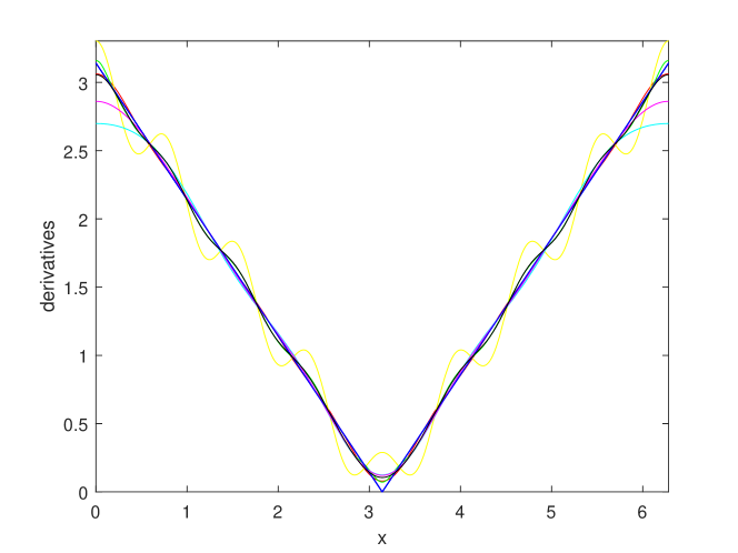
Example 8.2

Set

$$y(x)=\left\{\begin{array}[]{rcl}\pi x-\frac{1}{2}x^{2},\ 0\leq x<\pi,\\ \frac{1}{2}x^{2}-\pi x+\pi^{2},\pi\leq x<2\pi.\end{array}\right.$$

$$y(0)=0,$$

$$y^{\delta}(x)=y(x)+\delta\frac{\sin kx}{\sqrt{\pi}},$$

$$y^{\prime}(x)=\left\{\begin{array}[]{rcl}\pi-x,\ 0\leq x<\pi,\\ x-\pi,\pi\leq x<2\pi.\end{array}\in H^{1}_{per}(0,2\pi)\right.$$

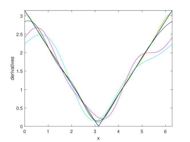
8.2.2 Second order

Example 8.3

Set

$$y(x)=\left\{\begin{array}[]{rcl}\frac{1}{2}\pi x^{2}-\frac{1}{6}x^{3},\ 0\leq x<\pi,\\ \frac{1}{6}x^{3}-\frac{1}{2}\pi x^{2}+\pi^{2}x-\frac{1}{3}\pi^{3},\pi\leq x<2\pi.\end{array}\right.$$

$$y(0)=0,\ y^{\prime}(0)=0$$

$$y^{\delta}(x)=y(x)+\delta\frac{\sin kx}{\sqrt{\pi}},$$

$$y^{\prime\prime}(x)=\left\{\begin{array}[]{rcl}\pi-x,\ 0\leq x<\pi,\\ x-\pi,\pi\leq x<2\pi.\end{array}\in H^{1}_{per}(0,2\pi)\right.$$

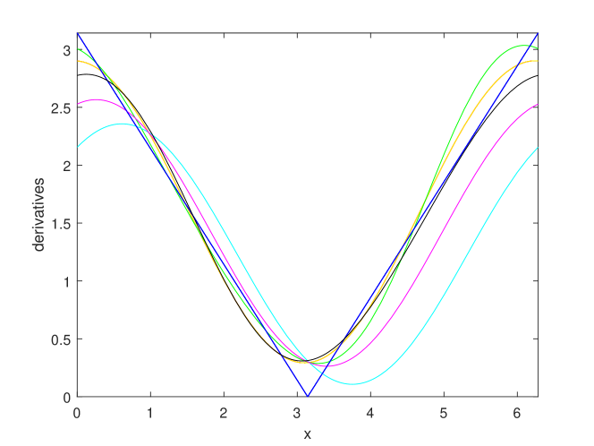
8.2.3 Third order

Example 8.4

Set

$$y(x)=\left\{\begin{array}[]{rcl}\frac{1}{6}\pi x^{3}-\frac{1}{24}x^{4},\ 0\leq x<\pi,\\ \frac{1}{24}x^{4}-\frac{1}{6}\pi x^{3}+\frac{1}{2}\pi^{2}x^{2}-\frac{1}{3}\pi^{3}x+\frac{1}{12}\pi^{4},\pi\leq x<2\pi.\end{array}\right.$$

$$y(0)=0,\ y^{\prime}(0)=0,\ y^{\prime\prime}(0)=0;$$

$$y^{\delta}(x)=y(x)+\delta\frac{\sin kx}{\sqrt{\pi}},$$

$$y^{\prime\prime\prime}(x)=\left\{\begin{array}[]{rcl}\pi-x,\ 0\leq x<\pi,\\ x-\pi,\pi\leq x<2\pi.\end{array}\in H^{1}_{per}(0,2\pi)\right.$$

Figure 1: The figure corresponds to Example 8.2 where the bule curve denotes the exact derivative, the red, yellow, green curves denote the case $(\delta,\delta_{i},n)=(0.1,0,7)$, $(\delta,\delta_{i},n)=(0.05,0,10)$ and $(\delta,\delta_{i},n)=(0.01,0,23)$ and the lightcyan, manganese purple, black curves denote the case $(\delta,\delta_{i},n)=(0.1,0.1,4)$, $(\delta,\delta_{i},n)=(0.05,0.05,5)$ and $(\delta,\delta_{i},n)=(0.01,0.01,12)$ respectively.

Figure 2: The figure corresponds to Example 8.3 where the bule curve denotes the exact derivative, the red, yellow, green curves denote the case $(\delta,\delta_{i},n)=(0.1,0,3)$, $(\delta,\delta_{i},n)=(0.05,0,3)$ and $(\delta,\delta_{i},n)=(0.01,0,6)$ and the lightcyan, manganese purple, black curves denote the case $(\delta,\delta_{i},n)=(0.1,0.1,2)$, $(\delta,\delta_{i},n)=(0.05,0.05,3)$ and $(\delta,\delta_{i},n)=(0.01,0.01,4)$ respectively.

Figure 3: The figure corresponds to Example 8.4 where the bule curve denotes the exact derivative, the red, yellow, green curves denote the case $(\delta,\delta_{i},n)=(0.1,0,1)$, $(\delta,\delta_{i},n)=(0.05,0,1)$ and $(\delta,\delta_{i},n)=(0.01,0,2)$ and the lightcyan, manganese purple, black curves denote the case $(\delta,\delta_{i},n)=(0.1,0.1,1)$, $(\delta,\delta_{i},n)=(0.05,0.05,1)$ and $(\delta,\delta_{i},n)=(0.01,0.01,2)$ respectively.

8.2.4 Unified observation on cases with periodic weakly differentiable derivative

In this subsection, we utilize strategies (6.4) and (7.1) to determine regularization parameter for two cases with different noise level respectively. The figures 1-3 show the good effectiveness of strategy proposed in this paper in a general aspect.

8.3 On discontinuous derivatives

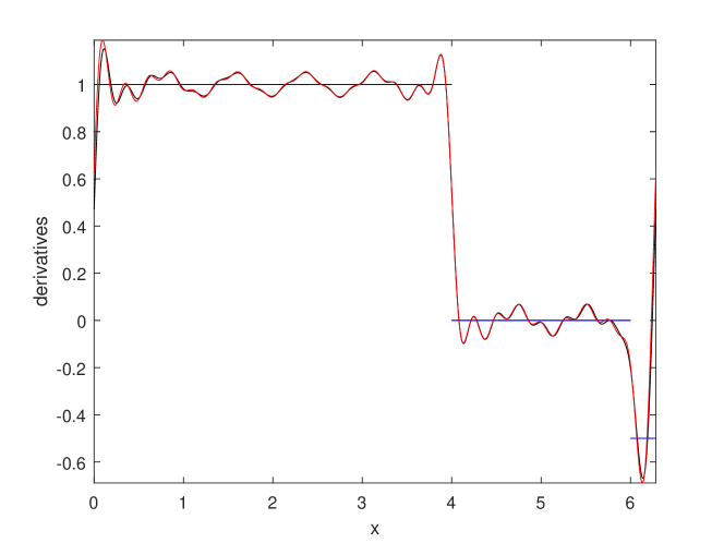
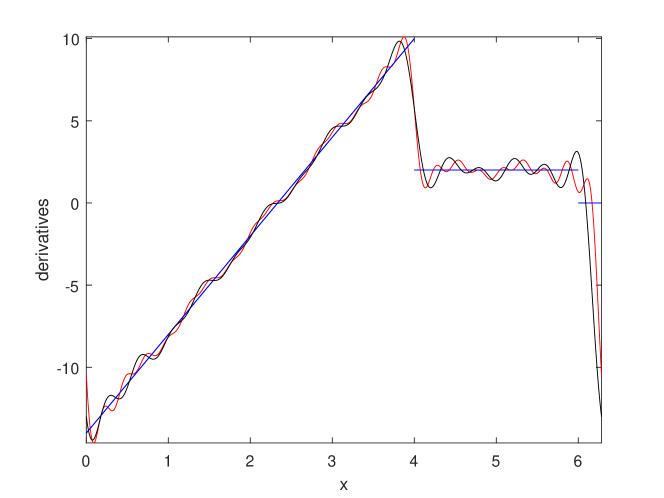
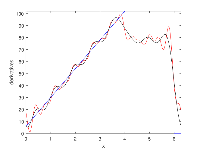
In the following numerical examples with non-periodic discontinuous derivatives, we choose to adjust parameter

$$n^{(p)}=n^{(p)}(\delta,\delta_{i}),\ p=1,2,3,$$

with experiments, not by (6.3) for the uncertainties to determine $\kappa$. Figures corresponding to least-error $r$ in numerical differentiation of each order are attached.

8.3.1 First order

Example 8.5

Set

$$y(x)=\left\{\begin{array}[]{rcl}x,\ 0\leq x<4,\\ 4,\ 4\leq x<6,\\ 7-\frac{x}{2},6\leq x<2\pi.\end{array}\right.$$

$$y(0)=0,$$

$$y^{\delta}(x)=y(x)+\delta\frac{\sin kx}{\sqrt{\pi}},$$

$$y^{\prime}(x)=\left\{\begin{array}[]{rcl}1,\ 0\leq x<4,\\ 0,\ 4\leq x<6,\\ -\frac{1}{2},6\leq x<2\pi.\end{array}\right.$$

8.3.2 Second order

Example 8.6

Set

$$y(x)=\left\{\begin{array}[]{rcl}x^{3}-7x^{2},\ 0\leq x<4,\\ x^{2}-16x,\ 4\leq x<6,\\ -4x-36,6\leq x<2\pi.\end{array}\right.$$

$$y(0)=0,y^{\prime}(0)=0,$$

$$y^{\delta}(x)=y(x)+\delta\frac{\sin kx}{\sqrt{\pi}},$$

$$y^{\prime\prime}(x)=\left\{\begin{array}[]{rcl}6x-14,\ 0\leq x<4,\\ 2,\ 4\leq x<6,\\ 0,6\leq x<2\pi.\end{array}\right.$$

8.3.3 Third order

Example 8.7

Set

$$y(x)=\left\{\begin{array}[]{rcl}x^{4}+x^{3},\ 0\leq x<4,\\ 13x^{3}-48x^{2}+64x,\ 4\leq x<6,\\ 186x^{2}-1340x+2808,6\leq x<2\pi.\end{array}\right.$$

$$y(0)=0,y^{\prime}(0)=0,y^{\prime\prime}(0)=0,$$

and

$$y^{\delta}(x)=y(x)+\delta\frac{\sin kx}{\sqrt{\pi}},$$

$$y^{\prime\prime\prime}(x)=\left\{\begin{array}[]{rcl}24x+6,\ 0\leq x<4,\\ 78,\ 4\leq x<6,\\ 0,6\leq x<2\pi.\end{array}\right.$$

		$n$	$4$	$6$	$8$	$16$	24
$p=1$	$\delta_{i}=0$	$r$	0.2786	0.2551	0.2294	0.1474	0.1294
	$\delta_{i}=0.01$	$r$	0.2734	0.2486	$0.2216$	$0.1378$	0.1187
$p=2$	$\delta_{i}=0$	$r$	0.4148	0.3175	0.2754	0.2068	0.1636
	$\delta_{i}=0.01$	$r$	0.4239	0.3323	0.2948	0.2603	0.2667
$p=3$	$\delta_{i}=0$	$r$	0.1413	0.1185	0.1209	0.1137	0.1490
	$\delta_{i}=0.01$	$r$	0.1446	0.1185	0.1060	0.1383	0.4010

Table 3: Above experiments correspond to Example 8.2, 8.3 and 8.4 respectively. Case I,II are uniformly set as $(\delta,\delta_{i})=(0.01,0)$ and $(\delta,\delta_{i})=(0.01,0.01)$ respectively. Notice that $r$ denotes the relative error. ($k=8$)

		$n$	$4$	$6$	$8$	$16$	24
$p=1$	$\delta_{i}=0$	$t$	1.73	2.67	3.89	12.47	103.05
	$\delta_{i}=0.01$	$t$	1.55	2.66	4.29	13.80	142.73
$p=2$	$\delta_{i}=0$	$t$	3.77	6.57	11.38	73.04	175.93
	$\delta_{i}=0.01$	$t$	3.95	6.46	11.09	116.55	230.05
$p=3$	$\delta_{i}=0$	$t$	6.10	13.06	19.47	127.01	304.70
	$\delta_{i}=0.01$	$t$	7.79	11.45	17.89	149.72	438.42

Table 4: $t$ denotes the CPU time $(s)$ for the corresponding experiments in Table 3.

Figure 4: The figure corresponds to Example 8.2 where the bule curve denotes the exact derivative, and the red, black curves denote the case $(\delta,\delta_{i},n)=(0.01,0,24)$ and $(\delta,\delta_{i},n)=(0.01,0.01,24)$ respectively.

Figure 5: The figure corresponds to Example 8.3 where the blue curve denotes the exact derivative, and the red, black curve denote the case $(\delta,\delta_{i},n)=(0.01,0,24)$ and $(\delta,\delta_{i},n)=(0.01,0.01,16)$ respectively.

Figure 6: The figure corresponds to Example 8.4 where the blue curve denote the exact derivative, and the red, black curves denote the case $(\delta,\delta_{i},n)=(0.01,0,16)$ and $(\delta,\delta_{i},n)=(0.01,0.01,8)$ respectively.

8.3.4 Unified observation on cases with discontinuous derivative

It can be concluded from figure 4,5,6 that, in both cases, when regularization parameters are chosen appropriately, the computational error can be well controlled. However, for sake of the intersection of frequency band of $y$ and $\delta y$ (this does not happen in the example we list in the subsection 8.1), the good filtering effect disappears in case with discontinuous derivative. Besides, we note that when the choice of $n$ increases to $\mathcal{U}:=\{16,24\}$, the CPU time will increase to a considerable amount.

9 Conclusion

The core theoretical work of this paper locates in the uniform upper estimate for

$$\|{A^{(p)}_{n}}^{\dagger}P_{n}A^{(p)}\|_{L^{2}\to L^{2}}$$

where $A^{(p)},A_{n}^{(p)}$ are defined in (2.4), (3.3) respectively. This determines the error estimate for approximation error and give a complete answer to regularization procedure.
In experiments, the algorithm has its advantage over other classical regularization method:

• It induces a noise-independent a-priori parameter choice strategy for function of a specific class

  $$y(t)=\sum^{N_{1}}_{k=1}a_{k}\cos kt+\sum^{N_{2}}_{k=1}b_{k}\sin kt+\sum^{p-1}_{k=0}c_{k}t^{k}$$

  where $p$ is the order of numerical differentiation. Good filtering effect (error approaches 0) is displayed when the algorithm acts on functions of above class with best parameter choice.

• Derivatives discontinuities can also be recovered well although there exists a unknown constant $\kappa$ to test in experiments.

Appendix A Representation of $M_{n}^{(p)}$

$$M_{n}^{(p)}=\left(\begin{array}[]{cccc}a^{(p)}&u^{(p)}_{1}&\cdots&u^{(p)}_{n}\\ {v^{(p)}_{1}}^{T}&M^{(p)}_{11}&\cdots&M^{(p)}_{1n}\\ \vdots&\vdots&\ddots&\vdots\\ {v^{(p)}_{n}}^{T}&M^{(p)}_{n1}&\cdots&M^{(p)}_{nn}\\ \end{array}\right)_{(2n+1)\times(2n+1)},\ p=1,2,3.$$

where

$$a^{(1)}=\pi,a^{(2)}=\frac{2\pi^{2}}{3},a^{(3)}=\frac{\pi^{3}}{3}$$

$$u^{(1)}_{k}=(0,\frac{\sqrt{2}}{k}),\ v^{(1)}_{k}=-u^{(1)}_{k}$$

$$u^{(2)}_{k}=(\frac{\sqrt{2}}{k^{2}},\frac{\sqrt{2}\pi}{k}),\ v^{(2)}_{k}=(\frac{\sqrt{2}}{k^{2}},-\frac{\sqrt{2}\pi}{k})$$

$$u^{(3)}_{k}=(\frac{\sqrt{2}\pi}{k^{2}},\frac{2\sqrt{2}\pi^{2}}{3\cdot k}-\frac{\sqrt{2}}{k^{3}}),\ v^{(3)}_{k}=(\frac{\sqrt{2}\pi}{k^{2}},-\frac{2\sqrt{2}\pi^{2}}{3\cdot k}+\frac{\sqrt{2}}{k^{3}}),1\leq k\leq n$$

$$M^{(1)}_{ij}=0,\forall i\neq j,$$

$$M^{(1)}_{ii}=\left(\begin{array}[]{cc}0&-\frac{1}{i}\\ \frac{1}{i}&0\\ \end{array}\right),\ 1\leq i\leq n.$$

$$M^{(2)}_{ij}=\left(\begin{array}[]{cc}0&0\\ 0&-\frac{1}{i\cdot j}\\ \end{array}\right),\ 1\leq i,j\leq n,\ i\neq j.$$

$$M^{(2)}_{ii}=\left(\begin{array}[]{cc}-\frac{1}{i^{2}}&0\\ 0&-\frac{3}{i^{2}}\\ \end{array}\right),\ 1\leq i\leq n.$$

$$M^{(3)}_{ij}=\left(\begin{array}[]{cc}0&\frac{2}{i^{2}\cdot j}\\ -\frac{2}{i\cdot j^{2}}&-\frac{2\pi}{i\cdot j}\\ \end{array}\right),\ 1\leq i,j\leq n,\ i\neq j.$$

$$M^{(3)}_{ii}=\left(\begin{array}[]{cc}0&\frac{3}{i^{3}}\\ -\frac{3}{i^{3}}&-\frac{2\pi}{i^{2}}\\ \end{array}\right),\ 1\leq i\leq n.$$

Appendix B Some Fourier expansions

Lemma B.1

For $A^{(p)}$ defined in (2.4), when $j\geq n+1$, set

$$(P_{n}A^{(p)}(\frac{\cos jt}{\sqrt{\pi}}))(x)=c^{(p)}_{0}\frac{1}{\sqrt{2\pi}}+\sum^{n}_{k=1}c^{(p)}_{k}\frac{\cos kx}{\sqrt{\pi}}+\sum^{n}_{k=1}d^{(p)}_{k}\frac{\sin kx}{\sqrt{\pi}},$$

Then Fourier coefficients are determined as follows:

$$c^{(1)}_{0}=c^{(1)}_{k}=d^{(1)}_{k}=0,\ k\in\overline{1,...,n},$$ (2.1)

$$c^{(2)}_{0}=\frac{\sqrt{2}}{j^{2}},c^{(2)}_{k}=0,d^{(2)}_{k}=0,\ k\in\overline{1,...,n},$$ (2.2)

$$c^{(3)}_{0}=\frac{\sqrt{2}\pi}{j^{2}},c^{(3)}_{k}=0,d^{(3)}_{k}=-\frac{2}{kj^{2}},\ k\in\overline{1,...,n}.$$ (2.3)

Lemma B.2

For $A^{(p)}$ defined in (2.4), when $j\geq n+1$, set

$$(P_{n}A^{(p)}(\frac{\sin jt}{\sqrt{\pi}}))(x)=s^{(p)}_{0}\frac{1}{\sqrt{2\pi}}+\sum^{n}_{k=1}s^{(p)}_{k}\frac{\cos kx}{\sqrt{\pi}}+\sum^{n}_{k=1}t^{(p)}_{k}\frac{\sin kx}{\sqrt{\pi}},$$

Then Fourier coefficients are determined as follows

$$s^{(1)}_{0}=\frac{\sqrt{2}}{j},\ s^{(1)}_{k}=0,\ t^{(1)}_{k}=0,\ k\in\overline{1,...,n},$$ (2.4)

$$s^{(2)}_{0}=\frac{\sqrt{2}\pi}{j},\ s^{(2)}_{k}=0,\ t^{(2)}_{k}=-\frac{2}{kj},\ k\in\overline{1,...,n},$$ (2.5)

$$s^{(3)}_{0}=\frac{2\sqrt{2}\pi^{2}}{3j}-\frac{\sqrt{2}}{j^{3}},\ s^{(3)}_{k}=\frac{2}{k^{2}j},\ t^{(3)}_{k}=-\frac{2\pi}{kj}\ k\in\overline{1,...,n}.$$ (2.6)

Appendix C Some Inequalities

Proposition C.1

Set $L_{n},K_{n},F_{n},T_{n}$ defined as in Theorem 4.1. Then

$$L^{-1}_{n}\in[10n,36n],$$ (3.1)

$$K_{n}\in[-\frac{2}{n},-\frac{1}{2n}],$$ (3.2)

$$F_{n}\in[\frac{\sqrt{2}}{n(2n+1)},\frac{4\sqrt{2}}{n(2n+1)}],$$ (3.3)

$$T_{n}\in[\frac{1}{396}\frac{1}{n}\frac{1}{2n+1},\frac{3}{40}\frac{1}{n(2n+1)}],\ n\geq 5.$$ (3.4)

References

- [1] A. Adams, J. F. Fournier: Sobolev Spaces. Second Edition, Academic Press, 2003.
- [2] A. Israel, T. Greville: Generalized Inverses Theory and Applications. Second Edition, Springer-Verlag, New York, 2003.
- [3] A. Kirsch: An Introduction to the Mathematical Theory of Inverse Problems. Springer, New York, 1996.
- [4] A. Ramm, A. Smirnova: On stable numerical differentiation. Math. Comput. 70, 1131-1153 (2001).
- [5] C. Evans, F. Gariepy: Measure theory and fine properties of functions, Studies in Advanced Mathematics. CRC Press, Boca Raton, FL, 1992.
- [6] C. Groetsch: Generalized inverses of Linear Operators, Marcel Dekker, New York, 1977.
- [7] C. Groetsch: On a regularization-Ritz method for Fredholm equations of the first kind. J. Integral Equations 4, 173-182 (1982).
- [8] C. Groetsch: The Theory of Tikhonov Regularization for Fredholm Equations of the First Kind. Pitman, Boston, 1984.
- [9] F. Dou, C. Fu, Y. Ma: A wavelet-Galerkin method for high order numerical differentiation. Appl. Math. Comput. 215, 3702-3712 (2010).
- [10] H. Engl, M. Hanke, A. Neubauer: Regularization of Inverse Problems. Kluwer, Dordrecht, 1996.
- [11] H. Egger, H. Engl: Tikhonov regularization applied to the inverse problem of option pricing: convergence analysis and rates. Inverse Problems 21, 1027-1045 (2005).
- [12] J. Cullum: Numerical differentiation and regularization. SIAM J. Numer. Anal. 8, 254-265 (1971).
- [13] M. Dehghan: Quasi-implicit and two-level explicit finite-difference procedures for solving the one-dimensional advection equation. Applied Mathematics and Computation 167 (2005) 46-67.
- [14] M. Dehghan: Numerical solution of the three-dimensional advection-diffusion equation. Applied Mathematics and Computation 150 (2004) 5-19.
- [15] M. Dehghan, M. Abbaszadeh: A finite difference/finite element technique with error estimate for space fractional tempered diffusion-wave equation. Computers and Mathematics with Applications 75 (8), (2018) 2903-2914.
- [16] M. Dehghan: Finite difference procedures for solving a problem arising in modeling and design of certain optoelectronic devices. Mathematics and Computers in Simulation 71 (2006) 16-30.
- [17] M. Hanke, O. Scherzer: Inverse problems light: numerical differentiation. Am. Math. Mon. 108, 512-521 (2001).
- [18] N. Du: Finite-dimensional approximation settings for infinite-dimensional Moore-Penrose inverses. SIAM J. Numer. Anal. 46, 1454-1482 (2008).
- [19] P. Assari, M. Dehghan: Solving a class of nonlinear boundary integral equations based on the meshless local discrete Galerkin (MLDG) method. Applied Numerical Mathematics 123 (2018) 137-158.
- [20] P. Assari, M. Dehghan: A Meshless Galerkin Scheme for the Approximate Solution of Nonlinear Logarithmic Boundary Integral Equations Utilizing Radial Basis Functions. Journal of Computational and Applied Mathematics 333 (2018) 362-381.
- [21] P. Assari, M. Dehghan: A Meshless Local Discrete Galerkin (MLDG) Scheme for Numerically Solving Two-Dimensional Nonlinear Volterra Integral Equations. Applied Mathematics and Computation 350 (2019) 249-265.
- [22] P. Assari: A Meshless Local Galerkin Method for the Numerical Solution of Hammerstein Integral Equations Based on the Moving Least Squares Technique. Journal of Applied Analysis and Computation 9 (2019) 75-104.
- [23] P. Mathe, S. Pereverzev: The use of higher order finite difference schemes is not dangerous. Journal of Complexity. 25, 3-10 (2009).
- [24] R. Kress: Linear Integral Equations, Springer-Verlag, Berlin, 1989.
- [25] T. Hein, B. Hofmann: On the nature of ill-posedness of an inverse problem arising in option pricing. Inverse Problems 19, 1319-1338 (2003).
- [26] T. Wei, Y. Hon, Y. Wang: Reconstruction of numerical derivatives from scattered noisy data. Inverse Problems 21, 657-672 (2005).
- [27] X. Wan, Y. Wang and M Yamamoto: Detection of irregular points by regularization in numerical differentiation and application to edge detection. Inverse Problems 22, 1089-1103 (2006).
- [28] Y. Wang, X. Jia, J. Cheng: A numerical differentiation method and its application to reconstruction of discontinuity. Inverse Problems 18, 1461-1476 (2002).