Applicability of coupling strength estimation for linear chains of restricted access

Abstract

The characterization of an unknown quantum system requires the Hamiltonian identification. The full access to the system, however, is usually restricted, hindering the direct retrieval of relevant parameters, and a reliable indirect estimation is usually required. In this work, the algorithm proposed by Burgarth et al. [Phys. Rev. A 79, 020305 (2009)], which allows estimating the coupling strengths in a linear chain by addressing only one end site, is further investigated. The scheme is numerically studied for states with chain structure, exploring its applicability against observational errors including the limited signal-noise ratio and the finite spectral width. The spectral distribution of the end state is shown to determine the applicability of the method, and reducing the loss from truncated spectral components is critical to realizing the robust reconstruction of coupling strengths.

I Introduction

The accurate control of the Hamiltonian of designed systems is always a prerequisite to carry out desired tasks, e.g., quantum computation Ladd et al. (2010); Bassett and Awschalom (2012) quantum communication Bose (2003) and quantum metrology Giovannetti et al. (2006, 2011). The systems are usually microscopic structures which are delicately engineered to realize specific functions. To verify and benchmark these fabricated structures, the characterization of the system via Hamiltonian identification is desired Cole (2015). Usually, the dynamics within the system are extremely complicated, and the probing access is often restricted. A delicately devised identification scheme is supposed to allow the sensible estimation of unknown parameters, reconstructing the Hamiltonian indirectly based on partially available information, e.g., the a priori knowledge about the structure of the quantum network, the initial state, or an accessible subset of observables, et al..

Under the challenge of complicated dynamics and restricted addressing resources, various identification algorithms have been developed aiming at experimental realizations. In a many-body system, the dynamical decoupling technique, which simplifies the problem by decoupling each pair of qubits from the rest, allows for the Hamiltonian identification with arbitrary long-range couplings between qubits Wang et al. (2015). Besides, the dynamics can be altered by tuning the control pulse that is applied to the probe spin, improving the precision of estimation scheme Kiukas et al. (2017); Liu and Yuan (2017). In a network of limited access, the identification scheme is intended to bridge the Hamiltonian parameters and the observables from accessible subsystem that are relatively easy to measure. The system realization theory is proposed for temporal record of the observables of a local subsystem Zhang and Sarovar (2014, 2015), which has been experimentally demonstrated on a liquid nuclear magnetic resonance quantum information processor Hou et al. (2017). Zeeman marker protocol shows that local field-induced spectral shifts can be used to estimate parameters in spin chains or networks Burgarth and Ajoy (2017). Also, when the graph infection rule is satisfied, the similar parameter estimation is also available utilizing the spectral information retrieved from a partially accessible spin Burgarth et al. (2009); Burgarth and Maruyama (2009).

In this work, we re-examine the estimation algorithm proposed in Burgarth et al. (2009), where the reconstruction of coupling strengths in a linear chain without the full access is considered. The procedure, probing the global properties from a local site, is similar to the estimation of spring constants in classical-harmonic oscillator chains. By accessing only the end of the linear chain, the algorithm allows deducing all coupling strengths from the data of associated spectral information. Nevertheless, the errors of the input data are inevitable and may significantly influence the reconstruction results. In this work, we focus on the applicability of the algorithm when the acquired initial data deviate from the actual values. The simulations show that the spectral distribution is an important indicator of the applicability of the algorithm. Examining the spectral distribution, the increasing number of spectral components that approach zero are likely to fail the reconstruction. The applicability depends on both the properties of individual system and conditions of measurement. The work is organized as followings. In Sec. II, the recursive relations among spectral coefficients and coupling strengths from adjacent sites are derived. In Sec. III, the robustness and the availability of the algorithm are discussed under different conditions when input errors are introduced.

II Theory of coupling strength estimation

We consider the state transfer within a system governed by the generic Schrödinger equation,

$$\dot{c}_{i}=-\mathrm{i}\varepsilon_{i}c_{i}-\mathrm{i}\sum_{k\sim i}J_{i,k}c_{k},$$ (1)

with $c_{i}$ the amplitude of state $|i\rangle$, $\varepsilon_{i}$ the energy and $J_{i,k}$ the coupling strength. The symbol "$\sim$" means the two states are coupled. With amplitude $c_{i}=\langle i|\Psi(t)\rangle$ represented spectrally, $c_{i}=\sum_{n}C_{i,n}\mathrm{e}^{-\mathrm{i}\lambda_{n}t}$, where $C_{i,n}=\langle i|\lambda_{n}\rangle\langle\lambda_{n}|\psi(0)\rangle$ is the spectral coefficient of mode $n$. The relation of $C_{i,n}$ among coupled states reads

$$C_{i,n}=\frac{1}{\lambda_{n}-\varepsilon_{i}}\sum_{k\sim i}J_{i,k}C_{k,n}.$$ (2)

The relation allows estimating the parameters using the information retrieved from a subset of states under the restricted-access condition. The simplest example is a linear chain as shown in Fig. 1, where only the leftmost state $|1\rangle$ is accessible. Given an $N$-state chain with energies $\varepsilon_{i}$ known, all coupling strengths $J_{i,i+1}$ can be reconstructed using the spectral information simply read from state $|1\rangle$.

Figure 1: Schematics of parameter estimation for a chain of $N$ states. Assuming that the access of the chain is restricted, only state $|1\rangle$, the left-most site of the chain, can be measured by the detector and all the rest (states $|2\rangle$, $|3\rangle$, …, $|N\rangle$) is concealed by a blackbox. Using the scheme of parameter estimation, however, all coupling strengths, $J_{i,i+1}$, can be estimated if the spectral information of $|1\rangle$ is available.

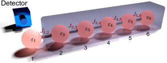
The feasibility of the scheme can be shown by the repetitive use of Eq. (2) and the normalization condition $\langle i|i\rangle=1$. Given the eigenmode $n$, the $C_{1,n}$ of left-most state $|1\rangle$ allows deriving $C_{2,n}$ of the next one,

$$C_{2,n}=\frac{\lambda_{n}-\varepsilon_{1}}{J_{12}}C_{1,n}.$$ (3)

Given that only $J_{i,k}$ with $k=i\pm 1$ are nonvanishing in a linear chain, the repetitive use of Eq. (2) yields coefficients of subsequent states recursively,

$$C_{i+1,n}=\frac{(\lambda-\varepsilon_{i})C_{i,n}-J_{i-1,i}C_{i-1,n}}{J_{i,i+1}}.$$ (4)

The denominator $J_{i,i+1}$ should be non-zero, since a "broken" coupling forbids the retrieval of the information on the further side. Eqs. (3) and (4) allow for the recursive evaluation of $C_{i+1,n}$ from $C_{i,n}$ and $C_{i-1,n}$.

On the other hand, the normalization condition $\langle i|i\rangle=1$ should be satisfied. With $C_{i,n}=\langle i|\lambda_{n}\rangle\langle\lambda_{n}|\psi(0)\rangle$, we have $\langle i|i\rangle=\sum_{n}\langle i|\lambda_{n}\rangle\langle\lambda_{n}|i\rangle=\sum_{n}|\frac{C_{i,n}}{\langle\lambda_{n}|\psi(0)\rangle}|^{2}=1.$ The unknown denominator $\langle\lambda_{n}|\psi(0)\rangle$ depends on the concrete form of initial state $|\psi(0)\rangle$. If the system is initially prepared by populating state $|1\rangle$ only, as considered in our case, $|\psi(0)\rangle=|1\rangle$, the denominator reads $|\langle\lambda_{n}|\psi(0)\rangle|^{2}=|\langle\lambda_{n}|1\rangle|^{2}=C_{1,n}$ and the normalization condition becomes

$$\langle i|i\rangle=\sum_{n}\frac{|C_{i,n}|^{2}}{C_{1,n}}=1.$$ (5)

With only state $|1\rangle$ accessible, the information of $|1\rangle$, $c_{1}(t)=\sum_{n}C_{1,n}\mathrm{e}^{-\mathrm{i}\lambda_{n}t}$, is supposed to be acquired by measurement, providing the input values of $C_{1,n}$ and $\lambda_{n}$ for further parameter estimation. The measured $C_{1,n}$ should be normalized by Eq. (5). Next, substituting Eq. (3) into Eq. (5) with $i=2$, the normalization condition $\langle 2|2\rangle=1$ yields

$$J_{1,2}=\sqrt{\sum_{n}^{N}|\lambda_{n}-\varepsilon_{1}|^{2}C_{1,n}}$$ (6)

and the normalized $C_{2,n}$ using Eq. (3). With the evaluated $J_{i-1,i}$, $C_{i,n}$ and $C_{i-1,n}$, Eq. (5) generates the $J_{i,i+1}$ for $i\geqslant 2$,

$$J_{i,i+1}=\sqrt{\sum_{n}^{N}\frac{|(\lambda_{n}-\varepsilon_{i})C_{i,n}-J_{i-1,i}C_{i-1,n}|^{2}}{C_{1,n}}}.$$ (7)

Hence, all coupling strengths can be recursively evaluated based on the above derived Eqs . (3), (4), (6) and (7).

In a realistic experimental setup, the above scheme works for any system that can be reduced to the form equivalent to Eq. (1). In Burgarth and Maruyama (2009), the method is applied to the spin chain described by Heisenberg Hamiltonian,

$$\hat{H}=\sum_{i}^{N-1}J_{i,i+1}(\sigma_{i}^{+}\sigma_{i+1}^{-}+\sigma_{i}^{-}\sigma_{i+1}^{+}+\Delta\sigma_{i}^{z}\sigma_{i+1}^{z})$$ (8)

with $\Delta$ the anisotropy. Assuming the system is prepared within the single excitation section, the subsequent evolution under the Hamiltonian (8) is still restricted to the single excitation sector. The time evolution is mapped to the generic Schrödinger equation for a single particle, Eq. (1), where the energies are given by $\varepsilon_{i}=\Delta\left[\sum_{j=1}^{N-1}J_{j,j+1}-2(J_{i,i+1}+J_{i-1,i})\right]$. Therefore, the above mentioned states $\{|i\rangle\}$, in this case, have been mapped to spatial sites. The values of $C_{1,n}$ are embedded in the reduced density matrix of $|1\rangle$, which can be experimentally obtained by quantum state tomography Burgarth and Maruyama (2009). Here, we are not concerned with the specific realization of the measurement, Hence, the input variables $\lambda_{n}$ and $C_{1,n}$ are assumed to be readily reachable, but they are not necessarily guaranteed to be completely precise, as will be discussed later.

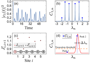
As a simple example, the estimation of $J_{i,i+1}$ in a chain with six sites is demonstrated in Fig. 2. Since the influence from disorder is not of concern in this work, all energies $\varepsilon_{i}$ are zero, as will also be considered in the following discussions. With only site $|1\rangle$ accessible, the time evolution of state $|1\rangle$ [Fig. 2(a)] is supposed to be detectable. In the associated spectral distribution [Fig. 2(b)], the position and the height of each spectral peak provide $\lambda_{n}$ and $C_{1,n}$, respectively, as required as input values by the estimation scheme. Performing the evaluation using Eqs . (3), (4), (6) and (7) recursively, we successfully reconstruct all the five unknown coupling strengths $J_{i,i+1}$, as shown in Fig. 2(c).

Figure 2: Reconstruction of $J_{i,i+1}$ for a chain of $N=6$ and $\varepsilon_{i}=0$. Panel (a) shows the temporal evolution of population on site 1, and (b) shows its spectral distribution that provides $\lambda_{n}$ and $C_{1,n}$ as required by the reconstruction algorithm. In (c), applying the parameter estimation, the five unknown coupling strengths are estimated. The estimated values $J_{i,i+1}^{\prime}$ show good agreement with the actual values $J_{i,i+1}$. Panel (d) presents the possible errors with the input values $\lambda_{n}$ and $C_{1,n}$ that may hamper the reconstruction procedure. For peak 1, the $C_{1,n}$ below the threshold during the measurement is simply truncated. For peak 2, the broadening of the spectral peak results in the deviation of the measured eigenvalue $\lambda_{n}^{\prime}$ from the actual $\lambda_{n}$.

III Influence from errors of input variables

During the actual measurement, the finite instrumental resolution, the limited signal-noise ratio and other perturbances may hinder the precise acquisition of initial input $\lambda_{n}$ and $C_{1,n}$. Therefore, the robustness of the algorithm against the deviations of these input values is critical to the success of the parameter estimation. The influence from imprecision of measured $C_{1,n}$ has been mentioned in Burgarth et al. (2009), showing rather robust performance against small deviations. When the finite signal-noise ratio of $C_{1,n}$ detection is considered, the even worse situation occurs when partial information are lost due to the truncation of small values. As is shown in Fig. 2(d), the finite signal-noise ratio sets the truncation threshold. As the value of $C_{1,n}$ for peak 1 is below the line representing the threshold, the corresponding $C_{1,n}$ is missing. Besides the errors in $C_{1,n}$ which are encoded in heights of spectral peaks, the $\lambda_{n}$ that are read from positions of peaks are also susceptible to errors during the measurement. As is shown by peak 2 in (d), the nonvanishing spectral width caused by either the finite instrumental resolution or the fluctuation during the measurement may contribute to the uncertainty $\Delta\lambda_{n}$. The imprecise $\lambda_{n}$ also deteriorate the performance of  $J_{i,i+1}$-reconstruction.

We take the example of the simplest parametric setup, a chain of 100 sites with identical coupling strengths $J_{i,i+1}=1$ and energies $\varepsilon_{i}=0$,  to show how the input values influence the results. Under the ideal condition without any deviations of $\lambda_{n}$ and $C_{1,n}$, the simulated results show the $J_{i,i+1}$ can be correctly recovered for a long chain (tested up to thousands sites). In a realistic experiment, however, the spectral peaks of small-valued $C_{1,n}$ may not be well resolved, or even simply be truncated. For the $n$th mode, when $C_{1,n}$ is zero, from Eqs. (3) and (4), all $C_{i,n}$ vanish, leading to the zero component in Eq. (7) without the associated contribution; and also, Eq. (7) is not bothered by the numerical difficulty of division by zero. However, with the less number of observed peaks than the actual number, the lost information does influence the reconstructed results.

Figure 3: For a homogeneous linear chain of $N=100$, panel (a) shows the spectral distribution $C_{1,n}$ versus $\lambda_{n}$. The region below $10^{-1}C_{\text{max}}$, as indicated by purple line in (a), is zoomed as shown in panel (b). Assuming the $C_{1,n}$ can be resolved up to $10^{-1}$ (purple), $10^{-2}$ (green) and $10^{-3}$ (red) of $C_{\text{max}}$, all the input data $(\lambda_{n},C_{1,n})$ with $C_{1,n}$ below the threshold are truncated. The corresponding estimated coupling strengths $J_{i,i+1}^{\prime}$ are shown in (c), (d) and (e), respectively, comparing with the original coupling strengths $J_{i,i+1}$.

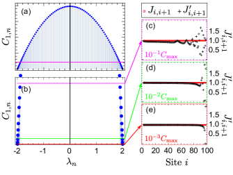
The influence from the truncation is shown in Fig. 3. For a homogeneous linear chain with all $\varepsilon_{i}=\varepsilon$ and $J_{i,i+1}=J$, the eigenvalues are given by $\lambda_{n}=\varepsilon+2J\cos[\pi n/(N+1)]$ for $n=1,\ldots,N$. The element of associated eigenvector for the $i$th site read $C_{i,n}=\sin[n\pi i/(N+1)]$. For the probing state $|1\rangle$, $C_{1,n}=\sin[n\pi/(N+1)]$, as is shown by the spectral distribution in Fig. 3(a). The $C_{1,n}$ of small values are around both the far ends along the $\lambda_{n}$-axis, where the data below a given threshold are truncated if a finite signal-noise ratio is specified. For different truncation thresholds as indicated in Fig. 3(b), the estimated results of $J_{i,i+1}$ are compared in Fig. 3(c)-(e).

Assuming that the maximum value of $C_{1,n}$ is $C_{\text{max}}$, when the threshold is $10^{-1}C_{\text{max}}$ with ten pairs of $C_{1,n}$ truncated, significant deviation appears from $i=50$. When the data below $10^{-2}C_{\text{max}}$ are truncated with three pairs of $C_{1,n}$ missing, the $J_{i,i+1}$ can be correctly reconstructed up to $i=80$. Further, when only one pair of data are truncated below the threshold $10^{-3}C_{\text{max}}$, the deviation only appear at the rightmost sites of the chain. The results suggest the complete data of $C_{1,n}$ should be important to the success of the algorithm. More intriguingly, though all $C_{1,n}$ contribute to the evaluation of each $J_{i,i+1}$, when some components are missing, the chain can still be recovered to some extent instead of failing the reconstruction as a whole, which shows the robustness of the algorithm.

Next, we consider the estimation when $J_{i,i+1}$ vary with $i$, as we desire in practice. Without loss of generality, the $J_{i,i+1}$ are randomly chosen within a given interval, i.e., the disorder induced by $J_{i,i+1}$. It is shown that the interval is highly relevant to the performance of the estimation. Figs. 4(a) and (b) present the dependence of the reconstruction on the interval. In (a), when the span is small, $J_{i,i+1}\in[0.9,1.1]$, the $J_{i,i+1}$ can be correctly estimated up to $i=28$. While when the span is large, $J_{i,i+1}\in[0.8,1.2]$, the applicability deteriorates—the estimated values $J^{\prime}_{i,i+1}$ starts deviating from $J_{i,i+1}$ around site 16, as can be straightforwardly read from the error defined by $\delta J_{i,i+1}=J^{\prime}_{i,i+1}-J_{i,i+1}$ as shown in Fig. 4(c).

Figure 4: Estimation of $J_{i,i+1}$ in a chain of $N=50$ when $C_{1,n}$ is resolved up to $10^{-3}$. The $J_{i,i+1}$ are randomly distributed in range (a) $[0.9,1.1]$  and (b) $[0.8,1.2]$. The errors $\delta J_{i,i+1}=J^{\prime}_{i,i+1}-J_{i,i+1}$ for the two different intervals are compared in panel (c). The different parametric ranges lead to distinguished spectral distributions, as shown in (d) and (e).

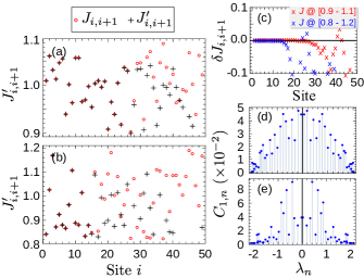
As discussed above, the reconstruction is rather robust for a long chain with identical $J_{i,i+1}$. When $J_{i,i+1}$ are randomly distributed, however, the effective distance of reconstruction is significantly shortened, showing an anticorrelation between the distance and the distribution interval of $J_{i,i+1}$. Examining the spectral distribution, the anticorrelation can also be explained by the truncation of $C_{1,n}$ as discussed for the homogeneous chain. The distribution interval of $J_{i,i+1}$ influences the spectral pattern and the probability to find $C_{1,n}$ around zero. With the distribution of random $J_{i,i+1}$ broadened, the spectral distribution Figs. 4(d) and (e) is no more as regular as that in the homogeneous chain. The $C_{1,n}$ scatter to a larger range with the increasing distribution interval of $J_{i,i+1}$, and more $C_{1,n}$ approach zero. As discussed for the homogeneous chain, these near-zero $C_{1,n}$ are likely to be truncated, and the resultant lost spectral components worsen the applicability of the algorithm. In addition, it is found that the decreasing  $J_{i,i+1}$ also lowers the value of $C_{1,n}$ and impedes the parameter estimation, as can be intuitively understood since any broken bridge hinders the probe of further sites. The above discussion also applies when disorders of $\varepsilon_{i}$ are involved as the spectral distribution also presents the similar pattern and suggests the involvement of the localization.

Besides the influence from errors of $C_{1,n}$, the measurement of $\lambda_{n}$ also affects the $J_{i,i+1}$ reconstruction. Assuming the actual eigenvalue is $\lambda_{n}$, the restricted resolution or disturbance during the experiment may deviate the measured value from $\lambda_{n}$, $\lambda_{n}^{\prime}=\lambda_{n}+\Delta\lambda_{n}$. The fluctuation $\Delta\lambda_{n}$ in each measurement results in the difference of estimated $J_{i,i+1}^{\prime}$, as illustrated in Fig. 2(d). The eventual $J_{i,i+1}^{\prime}$ should be the average of reconstructed results after multiple measurements. We sample 2000 random $\Delta\lambda_{n}$ of normal distribution, $\Delta\lambda_{n}\sim\mathcal{N}(0,\sigma^{2})$, to estimated the randomly distributed  $J_{i,i+1}\in[0.9,1.1]$ in a chain of $N=100$ as shown in Fig. 5(a). Here, the influence by the truncation of small-valued $C_{1,n}$ is neglected.

Figure 5: The estimation of coupling strengths when $\Delta\lambda_{n}$ is considered for each measurement. In a chain of 100 sites with $J_{i,i+1}\in[0.9,1.1]$, the reconstructed $J_{i,i+1}^{\prime}$ are compared with $J_{i,i+1}$ in (a) when $\Delta\lambda_{n}=0$. In (b), the reconstructed $J_{i,i+1}^{\prime}$ are shown when $\sigma=0.001$. The errors $\delta J_{i,i+1}$ are presented in (c), (d) and (e) for $\sigma=10^{-1}$, $10^{-2}$ and $10^{-3}$, respectively.

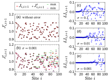
From the errors $\delta J_{i,i+1}$ as shown in Fig. 5(c), (d) and (e), the $J_{i,i+1}$ can be roughly estimated up to $i=20$, $40$ and $60$, respectively, for $\sigma=10^{-1}$, $10^{-2}$ and $10^{-3}$. While without $\Delta\lambda_{n}$ fluctuation [Fig. 5(a)], all $J_{i,i+1}$ are correctly reconstructed. Therefore, the precise measurement $\lambda_{n}$ is shown to be critical to the precise reconstruction. For a longer chain, we did not find significant deviations. However, the denser spectral distribution with more states involved will hinder the precise retrieval of $\lambda_{n}$, if the instrumental resolution of $\lambda_{n}$-acquisition is finite.

IV Conclusion

The reconstruction of parameters within a partially accessible system is an important problem when indirect probing is the only option to acquire the desired information. In this work, the algorithm to estimate parameters in a linear chain is investigated. Starting with the generic Schrödinger equation, it is confirmed that the coupling strengths can be efficiently deduced from the recursive relation using the spectral information of only the end site. We focus on the applicability of the algorithm, which is shown to be highly relevant to the spectral distribution on the accessible state. Given the errors induced by the finite signal-noise ratio, the increasing number of truncated spectral components are shown to gradually deteriorate the reconstruction performance. It is found that reducing the loss of spectral components is critical to the success of the method. Even so, the partially successful estimation in the presence of truncations shows the robustness of the algorithm and the estimation can be conducted in a controllable way. Since the spectral distribution is system dependent, the applicability of the method also varies with systems. Accordingly, it is advisable to understand the nature of the system before applying the method.