Generalized Minkowski sets for the regularization of inverse problems.

Abstract

Many works on inverse problems in the imaging sciences consider regularization via one or more penalty functions or constraint sets. When the models/images are not easily described using one or a few penalty functions/constraints, additive model descriptions for regularization lead to better imaging results. These include cartoon-texture decomposition, morphological component analysis, and robust principal component analysis; methods that typically rely on penalty functions. We propose a regularization framework, based on the Minkowski set, that merges the strengths of additive models and constrained formulations. We generalize the Minkowski set, such that the model parameters are the sum of two components, each of which is constrained to an intersection of sets. Furthermore, the sum of the components is also an element of another intersection of sets. These generalizations allow us to include multiple pieces of prior knowledge on each of the components, as well as on the sum of components, which is necessary to ensure physical feasibility of partial-differential-equation based parameters estimation problems. We derive the projection operation onto the generalized Minkowski sets and construct an algorithm based on the alternating direction method of multipliers. We illustrate how we benefit from using more prior knowledge in the form of the generalized Minkowski set using seismic waveform inversion and video background-anomaly separation.

1 Introduction

The inspiration for this work is twofold. First, we want to build on the success of the regularization of inverse problems in the imaging sciences using intersections of constraint sets. This approach may be in the form of minimizing a differentiable function $f(m):\mathbb{R}^{N}\rightarrow\mathbb{R}$, such that the estimated model parameters, $m\in\mathbb{R}^{N}$ are an element of the intersection of $p$ convex and possibly non-convex sets, $\bigcap_{i=1}^{p}\mathcal{C}_{i}$. The corresponding optimization problem reads $\min_{m}f(m)\>\>\text{s.t.}\>\>m\in\bigcap_{i=1}^{p}\mathcal{C}_{i}$. See, e.g., [Gragnaniello et al., 2012, Pham et al., 2014a, b, Smithyman et al., 2015, Peters and Herrmann, 2017, Esser et al., 2018, Yong et al., 2018, Peters et al., 2018]. Alternatively, we can also formulate certain types of inverse problems directly as a feasibility (also known as set-theoretic estimation) or projection problem [Youla and Webb, 1982, Trussell and Civanlar, 1984, Combettes, 1993, 1996]. This approach solves $\min_{m}1/2\|x-m\|_{2}^{2}\>\>\text{s.t.}\>\>m\in\bigcap_{i=1}^{p}\mathcal{C}_{i}$ or seeks any $m\in\bigcap_{i=1}^{p}\mathcal{C}_{i}$. The mentioned regularization techniques describe each piece of prior knowledge about the model parameters $m$ as a set. However, prior knowledge represented as a single set or as an intersection of different sets may not capture all we know. For instance, if the model contains oscillatory as well as blocky features. Because these are fundamentally different properties, working with one or multiple constraint sets alone may not able to express the simplicity of the entire model.

Motivated by ideas from cartoon-texture decomposition (CTD) and morphological component analysis (MCA) [Osher et al., 2003, Schaeffer and Osher, 2013, Starck et al., 2005, Ono et al., 2014] and robust or sparse principal component analysis (RPCA) [Candès et al., 2011, Gao et al., 2011a, b], we consider an additive model structure. Additive model structures decompose $m$ into two or more components—e.g., into a blocky cartoon-like component $u\in\mathbb{R}^{N}$ and an oscillatory texture-like component $v\in\mathbb{R}^{N}$. For this purpose, a penalty method is often used to state the decomposition problem as

$$\min_{u,v}\|m-u-v\|+\frac{\alpha}{2}\|Au\|+\frac{\beta}{2}\|Bv\|.$$ (1)

While this method has been successful, it requires careful choices for the penalty parameters $\alpha>0$ and $\beta>0$. These parameters determine how ‘much’ of $m$ ends up in each component, but also depend on the noise level. In addition, the values of these parameters relate to the choices for the norms and the linear operators $A\in\mathbb{C}^{M_{1}\times N}$ and $B\in\mathbb{C}^{M_{2}\times N}$. In this work, we are concerned with regularizing inverse problems by including multiple pieces of prior knowledge. For additive models, this means the number of terms in the sum and thus the number of penalty parameters will increase rapidly.

A constrained formulation can partially avoid the difficulties of selecting numerous penalty parameters because each constraint set can be defined independently of all other sets. This is contrary to penalty methods where the penalty parameters are trade-offs between the different penalty functions. Therefore, we explore the use of Minkowski sets for regularizing inverse problems. We require that the vector of model parameters, $m$, is an element of the Minkowski set $\mathcal{V}$, or vector sum of two sets $\mathcal{C}_{1}$ and $\mathcal{C}_{1}$, which is defined as

$$\mathcal{V}\equiv\mathcal{C}_{1}+\mathcal{C}_{1}=\{m=u+v\>|\>u\in\mathcal{C}_{1},v\in\mathcal{C}_{2}\}.$$ (2)

A vector $m$ is an element of $\mathcal{V}$ if it is the sum of vectors $u\in\mathcal{C}_{1}$ and $v\in\mathcal{C}_{2}$. Each set describes particular model properties for each component. Examples are total-variation, sparsity in a transform domain (Fourier, wavelets, curvelets, shearlets) or matrix rank. For practical reasons, we assume that all sets, sums of sets, and intersections of sets are non-empty, which implies that projection and feasibility problems have at least one solution. Our algorithm design uses the property that the sum of $p$ sets $\mathcal{C}_{i}$ is convex if all $\mathcal{C}_{i}$ are convex [Hiriart-Urruty and Lemaréchal, 2012, p. 24]. We apply our set-based regularization to imaging inverse problems with the Euclidean projection operator:

$$\mathcal{P}_{\mathcal{V}}(m)\in\mathop{\rm arg\min}_{x}\frac{1}{2}\|x-m\|_{2}^{2}\quad\text{s.t}\quad x\in\mathcal{V}.$$ (3)

This projection allows us to use Minkowski constraint sets in algorithms such as (spectral) projected gradient [SPG, Birgin et al., 1999], projected quasi-Newton [PQN, Schmidt et al., 2009], projected Newton algorithms [Bertsekas, 1982, Schmidt et al., 2012], and proximal-map based algorithms if we include the Minkowski constraint as an indicator function. We define this indicator function for a set $\mathcal{V}$ as

$$\iota_{\mathcal{V}}(m)=\begin{cases}0&\text{if }m\in\mathcal{V},\\ +\infty&\text{if }m\notin\mathcal{V},\\ \end{cases}$$ (4)

and the proximal map for a function $g(m):\mathbb{R}^{N}\rightarrow\mathbb{R}\cup\{+\infty\}$ as $\operatorname{prox}_{\gamma,g}(m)=\mathop{\rm arg\min}_{x}g(x)+\frac{\gamma}{2}\|x-m\|_{2}^{2}$, with $\gamma>0$. The proximal map for the indicator function of a set is the projection: $\operatorname{prox}_{\gamma,\iota_{\mathcal{V}}}(m)=\mathcal{P}_{\iota_{\mathcal{V}}}(m)$.

While Minkowski sets and additive models are powerful regularizers, they lack certain critical features needed for solving problems that involve physical parameters. For instance, there is, in general, no guarantee that the sum of two or more components lies within lower and upper bounds or satisfies other crucial constraints that ensure physically realistic model estimates. It is also not straightforward to include multiple pieces of prior information on each component.

1.1 Related work

The above introduced decomposition strategies, morphological component analysis or cartoon-texture [Osher et al., 2003, Schaeffer and Osher, 2013, Starck et al., 2005, Ono et al., 2014] and robust or sparse principal component analysis [Candès et al., 2011, Gao et al., 2011a, b]), share the additive model construction with multiscale decompositions in image processing [e.g., Meyer, 2001, Tadmor et al., 2004]. While each of the sets that appear in a Minkowski sum can describe a particular scale, this is not our primary aim or motivation. We use the summation structure to build more complex models out of simpler ones, more aligned with cartoon-texture decomposition and robust principal component analysis.

Projections onto Minkowski sets also appear in computational geometry, collision detection, and computer-aided design [e.g., Dobkin et al., 1993, Varadhan and Manocha, 2006, Lee et al., 2016], but the problems and applications are different. In our case, sets describe model properties and prior knowledge in $\mathbb{R}^{N}$. In computational geometry, sets are often the vertices of polyhedral objects in $\mathbb{R}^{2}$ or $\mathbb{R}^{3}$ and do not come with closed-form expressions for projectors or the Minkowski sum. We do not need to form the Minkowski set explicitly, and we show that projections onto the set are sufficient to regularize inverse problems.

1.2 Contributions and outline

We propose a constrained regularization approach suitable for inverse problems with an emphasis on physical parameter estimation, where we describe the model parameters using multiple components. This implies that we need to work with multiple constraints for each component while offering assurances that the sum of the components also adheres to certain constraints. For this purpose, we introduce a generalization of the Minkowski set and a formulation void of penalty parameters. We formulate the projection on such generalized Minkowski sets and construct an algorithm based on the alternating direction method of multipliers, including a discussion on important algorithmic details. We show how to use the projector to formulate inverse problems based on these sets.

The algorithms and numerical example are available as an open-source software package written in Julia. The algorithms and software are suitable for small 2D models, as well as for larger 3D geological models or videos, as we will show in the numerical examples section using seismic parameter estimation and video processing examples. These examples also demonstrate that the developed constrained problem formulation, algorithm, and software allow us to define constraints based on the entire 2D/3D model, but also simultaneously on slices/rows/columns/fibers of that model. This feature enables us to include more prior knowledge more directly into the inverse problem.

2 Generalized Minkowski set

It is challenging to select a single constraint set or intersection of multiple sets to describe models and images that contain distinct morphological components $u$ and $v$. While the Minkowski set allows us to define different constraint sets for the different components, limitations come to light when working with physical parameter estimation applications.

For instance, there is usually prior knowledge about the physically realistic values in $m\in\mathbb{R}^{N}$. Moreover, the successful applications of constrained formulations that we discussed in the introduction all use multiple constraints on the model parameters, and we want to combine that concept with constraints on the components.

The second extension of the basic concept of a Minkowski set is that we allow the constraint set on each component to be an intersection of multiple sets as well. In this way, we can include multiple pieces of prior information about each component.

We propose the generalized Minkowski constraint set for the regularization of inverse problems as

Definition 1 (Generalized Minkowski Set).

A vector $m\in\mathbb{R}^{N}$ is an element of the generalized Minkowski set,

$$\mathcal{M}\equiv\{m=u+v\>|\>u\in\bigcap_{i=1}^{p}\mathcal{D}_{i},\>v\in\bigcap_{j=1}^{q}\mathcal{E}_{j},\>m\in\bigcap_{k=1}^{r}\mathcal{F}_{k}\},$$ (5)

if $m$ is an element of the intersection of $r$ sets $\mathcal{F}_{k}$ and also the sum of two components $u\in\mathbb{R}^{N}$ and $v\in\mathbb{R}^{N}$. The vector $u$ is an element of the intersection of $p$ sets $\mathcal{D}_{i}$ and $v$ is an element of the intersection of $q$ sets $\mathcal{E}_{j}$.

The convexity of $\mathcal{M}$ follows from the properties of the sets $\mathcal{D}_{i}$, $\mathcal{E}_{j}$ and $\mathcal{F}_{k}$.

Proposition 1.

The generalized Minkowski set is convex if $\mathcal{D}_{i}$, $\mathcal{E}_{j}$ and $\mathcal{F}_{k}$ are convex sets for all $i$, $j$ and $k$.

Proof.

It follows directly from the definition that $\bigcap_{i=1}^{p}\mathcal{D}_{i}$, $\bigcap_{j=1}^{q}\mathcal{E}_{j}$, and $\bigcap_{k=1}^{r}\mathcal{F}_{k}$ are convex sets. As a result, the Minkowski sum $\bigcap_{i=1}^{p}\mathcal{D}_{i}+\bigcap_{j=1}^{q}\mathcal{E}_{j}$ is is also convex by because it is the sum of two convex sets [Hiriart-Urruty and Lemaréchal, 2012, p. 24]. Finally, It follows that $\mathcal{M}$ is a convex set, because it is the intersection of the convex intersection $\bigcap_{k=1}^{r}\mathcal{F}_{k}$, and the convex sum $\bigcap_{i=1}^{p}\mathcal{D}_{i}+\bigcap_{j=1}^{q}\mathcal{E}_{j}$. ∎

To summarize in words, $m$ is an element of the intersection of two convex sets, one is the convex Minkowski sum, the other is a convex intersection. The set $\mathcal{M}$ is therefore also convex. Note that convexity and closedness of $\bigcap_{i=1}^{p}\mathcal{D}_{i}$ and $\bigcap_{j=1}^{q}\mathcal{E}_{j}$ does not imply their sum is closed.

It is conceptually straightforward to extend set definition (5) to a sum of three or more components, but we work with two components for the remainder of this paper for notational convenience. In the discussion section, we highlight some potential computational challenges that come with a generalized Minkowski sets of more than two components.

3 Projection onto the generalized Minkowski set

In the following section, we show how to use the generalized Minkowski set, Equation (5), to regularize inverse problems with computationally cheap or expensive forward operators. First, we need to develop an algorithm to compute the projection onto $\mathcal{M}$. Using the projection operator, $\mathcal{P}_{\mathcal{M}}(\cdot)$, we can formulate inverse problems as a projection directly. Alternatively, we can use the projection operator inside projected gradient/Newton-type algorithms. Each constraint set definition may include a linear operator (the transform-domain operator) in its definition. We make the linear operators explicit, because the projection operator corresponding to, for example, $\{x\>|\>\|x\|_{2}\leq\sigma\}$, is available in closed form and easy to compute, but the projection onto $\{x\>|\>\|Ax\|_{2}\leq\sigma\}$ is not when $AA^{T}\neq\alpha I$ for $\alpha>0$, see examples in, e.g., Combettes and Pesquet [2011], Parikh and Boyd [2014], Beck, 2017, ch. 6 & 7, Diamond et al. [2018]. Let us introduce the linear operators $A_{i}\in\mathbb{R}^{M_{i}\times N}$, $B_{j}\in\mathbb{R}^{M_{j}\times N}$, and $C_{k}\in\mathbb{R}^{M_{k}\times N}$. With indicator functions and exposed linear operators, we formulate the projection of $m\in\mathbb{R}^{N}$ onto set (5) as

$$\min_{u,v,w}\frac{1}{2}\|w-m\|_{2}^{2}+\sum_{i=1}^{p}\iota_{\mathcal{D}_{i}}(A_{i}u)+\sum_{j=1}^{q}\iota_{\mathcal{E}_{j}}(B_{j}v)+\sum_{k=1}^{r}\iota_{\mathcal{F}_{k}}(C_{k}w)+\iota_{w=u+v}(w,u,v),$$ (6)

where $\iota_{w=u+v}(w,u,v)$ is the indicator function for the equality constraint $w=u+v$ that occurs in the definition of $\mathcal{M}$. The sets $\mathcal{D}_{i}$, $\mathcal{E}_{j}$, and $\mathcal{F}_{k}$ have the same role as in the previous section. The above problem is the minimization of a sum of functions acting on different as well as shared variables. We recast it in a standard form such that we can solve it using algorithms based on the alternating direction method of multipliers [ADMM, e.g., Boyd et al., 2011, Eckstein and Yao, 2015]. Rewriting in a standard form allows us to benefit from recently proposed schemes for selecting algorithm parameters that decrease the number of iterations and lead to more robust algorithms in case we use non-convex sets [Xu et al., 2016, 2017b]. As a first step, we introduce the vector $x\in\mathbb{R}^{2N}$ that stacks two out of the three optimization variables in (6) as

$$\begin{split}x\equiv\begin{pmatrix}u\\ v\end{pmatrix}.\end{split}$$ (7)

We substitute this new definition in Problem (6) and eliminate the equality constraints $w=u+v$ to arrive at

$$\min_{x}\frac{1}{2}\|\begin{pmatrix}I_{N}\>\>\>I_{N}\end{pmatrix}x-m\|_{2}^{2}+\sum_{i=1}^{p}\iota_{\mathcal{D}_{i}}(\begin{pmatrix}A_{i}\>\>\>0\end{pmatrix}x)+\sum_{j=1}^{q}\iota_{\mathcal{E}_{j}}(\begin{pmatrix}0\>\>\>B_{j}\end{pmatrix}x)+\sum_{k=1}^{r}\iota_{\mathcal{F}_{k}}(\begin{pmatrix}C_{k}\>\>\>C_{k}\end{pmatrix}x),$$ (8)

where $0_{M_{i}\times N}\in\mathbb{R}^{M_{i}\times N}$ indicate all zeros matrices of appropriate dimensions. Next, we take the linear operators out of the indicator function such that we end up with sub-problems that are usually projections with closed-form solutions. Thereby we avoid the need for nesting iterative algorithms to solve sub-problems related to the indicator functions of constraint sets.

To separate indicator functions and linear operators, we introduce additional vectors $y_{i}$ for $i\in\{1,2,\dots,p+q+r+1\}$ of appropriate dimensions. From now on we use $s=p+q+r+1$ to shorten notation. With the new variables, we rewrite problem formulation (8) and add linear equality constraints to obtain

$$\min_{\{y_{i}\},x}\frac{1}{2}\|y_{s}-m\|_{2}^{2}+\sum_{i=1}^{p}\iota_{\mathcal{D}_{i}}(y_{i})+\sum_{j=1}^{q}\iota_{\mathcal{E}_{j}}(y_{j+p})+\sum_{k=1}^{r}\iota_{\mathcal{F}_{k}}(y_{k+p+q})\>\>\text{s.t.}\>\>\tilde{A}x=\tilde{y},$$ (9)

where

$$\tilde{A}x=\tilde{y}\Leftrightarrow\begin{pmatrix}A_{1}&0\\ \vdots&0\\ A_{p}&0\\ 0&B_{1}\\ 0&\vdots\\ 0&B_{q}\\ C_{1}&C_{1}\\ \vdots&\vdots\\ C_{r}&C_{r}\\ I_{N}&I_{N}\\ \end{pmatrix}\begin{pmatrix}u\\ v\end{pmatrix}=\begin{pmatrix}y_{1}\\ \vdots\\ y_{p}\\ y_{p+1}\\ \vdots\\ y_{p+q}\\ y_{p+q+1}\\ \vdots\\ y_{p+q+r}\\ y_{p+q+r+1}\\ \end{pmatrix}.$$

Now define the new function

$$\tilde{f}(\tilde{y},m)\equiv\sum_{i=1}^{s}f_{i}(y_{i},m)\equiv\frac{1}{2}\|y_{s}-m\|_{2}^{2}+\sum_{i=1}^{p}\iota_{\mathcal{D}_{i}}(y_{i})+\sum_{j=1}^{q}\iota_{\mathcal{E}_{j}}(y_{j+p})+\sum_{k=1}^{r}\iota_{\mathcal{F}_{k}}(y_{k+p+q}),$$ (10)

such that we obtain the projection problem in the form

$$\min_{x,\tilde{y}}\tilde{f}(\tilde{y},m)\>\>\text{s.t.}\>\>\tilde{A}x=\tilde{y}.$$ (11)

If $x$ and $\tilde{y}$ are a solution to this problem, the equality constraints enforce $u+v=y_{p+q+r+1}$ and we recover the projection of $m$ as $y_{p+q+r+1}$ or as $\begin{pmatrix}I_{N}\>\>I_{N}\end{pmatrix}x$. Now that Problem (11) is in a form that we can solve with the ADMM algorithm, we proceed by writing down the augmented Lagrangian for Problem (11) [Nocedal and Wright, 2000, Chapter 17] as

$$L_{\rho_{1},\dots,\rho_{s}}(x,y_{1},\dots,y_{s},v_{1},\dots,v_{s})=\sum_{i=1}^{s}\bigg{[}f_{i}(y_{i})+v_{i}^{T}(y_{i}-A_{i}x)+\frac{\rho_{i}}{2}\|y_{i}-A_{i}x\|^{2}_{2}\bigg{]},$$ (12)

where $\rho_{i}>0$ are the augmented Lagrangian penalty parameters and $v_{i}\in\mathbb{R}^{M_{i}}$ are the vectors of Lagrangian multipliers. We denote a block-row of the matrix $\tilde{A}$ as $A_{i}$. The relaxed ADMM iterations with relaxation parameters $\gamma_{i}\in(0,2]$ and iteration counter $l$ are given by

$$x^{l+1}=\arg\min_{x}\sum_{i=1}^{s}\frac{\rho_{i}^{l}}{2}\|y_{i}^{l}-A_{i}x+\frac{v_{i}^{l}}{\rho_{i}^{l}}\|^{2}_{2}=\Big{[}\sum_{i=1}^{s}(\rho_{i}^{l}A_{i}^{T}A_{i})\Big{]}^{-1}\sum_{i=1}^{s}\Big{(}A_{i}^{T}(\rho_{i}^{l}y_{i}^{l}+v_{i}^{l})\Big{)}$$

$$\text{compute for}\>\>i\in\{1,\dots,s\}\>\>\text{independently in parallel:}$$

$$\bar{x}_{i}^{l+1}=\gamma_{i}^{l}A_{i}x_{i}^{l+1}+(1-\gamma_{i}^{l})y_{i}^{l}$$ (13)

$$y_{i}^{l+1}=\arg\min_{y_{i}}\Big{[}f_{i}(y_{i})+\frac{\rho_{i}^{l}}{2}\|y_{i}^{l}-\bar{x}_{i}^{l+1}+\frac{v_{i}^{l}}{\rho_{i}^{l}}\|^{2}_{2}\Big{]}=\operatorname{prox}_{f_{i},\rho_{i}}(\bar{x}_{i}^{l+1}-\frac{v_{i}^{l}}{\rho_{i}^{l}})$$

$$v_{i}^{l+1}=v_{i}^{l}+\rho_{i}^{l}(y_{i}^{l+1}-\bar{x}_{i}^{l+1}).$$

These iterations are similar to the Simultaneous Direction Method of Multipliers [SDMM, Combettes and Pesquet, 2011, Kitic et al., 2016]) and the SALSA algorithm [Afonso et al., 2011]. The difference is that we have an additional relaxation step and use a separate augmented Lagrangian penalty parameter and relaxation parameter for each index $i$ that corresponds to a different set. The structure of these iterations look identical to the algorithm presented by Peters and Herrmann [2019] to compute the projection onto an intersection of sets, but here we solve a different problem and have different block-matrix structures. We briefly mention the main properties of each sub-problem.

$x^{l+1}$ computation. This step is the solution of a large, sparse, square, and symmetric linear system. The system matrix has the following block structure:

$$Q\equiv\sum_{i=1}^{s}(\rho_{i}A_{i}^{T}A_{i})=$$ (14)

$$\begin{pmatrix}\sum_{i=1}^{p}\rho_{i}A_{i}^{T}A_{i}+\sum_{k=1}^{r}\rho_{k}C_{k}^{T}C_{k}+\rho_{s}I_{N}&\sum_{k=1}^{r}\rho_{k}C_{k}^{T}C_{k}+\rho_{s}I_{N}\\ \sum_{k=1}^{r}\rho_{k}C_{k}^{T}C_{k}+\rho_{s}I_{N}&\sum_{j=1}^{q}\rho_{j}B_{j}^{T}B_{j}+\sum_{k=1}^{r}\rho_{k}C_{k}^{T}C_{k}+\rho_{s}I_{N}\end{pmatrix}.$$

This matrix is positive-definite if $\tilde{A}$ has full column rank. We assume this is true in the remainder because we always use bound constraints on each of the components. This implies that at least one of the $A_{i}$ and one of the $B_{i}$ is the identity matrix, which makes $Q$ positive-definite. We compute $x^{l+1}$ with the conjugate gradient (CG) method, warm started by $x^{l}$ as the initial guess. We choose CG instead of an iterative method for least-squares problems such as LSQR [Paige and Saunders, 1982] because solvers for least-squares work with $A$ and $A^{T}$ separately and need to compute a matrix-vector product (MVP) with each $A_{i}$ and $A_{i}^{T}$ at every iteration. This becomes computationally expensive if there are many linear operators, as is the case for our problem. CG uses a single MVP with $Q$ per iteration. The cost of this MVP does not increase if we add orthogonal matrices to $\tilde{A}$ (DCT, DFT, various wavelet transforms). If the matrices in $\tilde{A}$ have (partially) overlapping sparsity patterns (matrices based on discrete derivatives for exmple), the cost also does not increase (much). We pre-compute all $A_{i}^{T}A_{i}$ for fast updating of $Q$ when one or more of the $\rho_{i}$ change (see below).

$y_{i}^{l+1}$ computation. For every index $i$, we can compute $\operatorname{prox}_{f_{i},\rho_{i}}(\bar{x}_{i}^{l+1}-\frac{v_{i}^{l}}{\rho_{i}^{l}})$ independently in parallel. For indices $i\in\{1,2,\dots,s-1\}$, the proximal maps are projections onto sets $\mathcal{D}$, $\mathcal{E}$ or $\mathcal{F}$. These projections do not include linear operators, and we know the solutions in closed form (e.g., $\ell_{1}$-norm, $\ell_{2}$-norm, rank, cardinality, bounds).

$\rho_{i}^{l+1},\gamma_{i}^{l+1}$ updates. We use the updating scheme for $\rho$ and $\gamma$ from adaptive-relaxed ADMM, introduced by Xu et al. [2017b]. Numerical results show that this updating scheme accelerates the convergence of ADMM [Xu et al., 2017a, b, c], also is also robust when solving some non-convex problems [Xu et al., 2016]. We use a different relaxation and penalty parameter for each function $f_{i}(y_{i})$, as do Song et al. [2016]; Xu et al. [2017c], which allows $\rho_{i}$ and $\gamma_{i}$ to adapt to the various linear operators of different dimensions that correspond to each constraint set.

Parallelism and communication. The only serial part of the algorithm defined in (3) is the $x^{l+1}$ computation. We use multi-threaded MVPs in the compressed diagonal format if $Q$ has a banded structure. The other parts of the iterations, $y_{i}^{l+1}$, $v_{i}^{l+1},`\rho_{i}^{l+1},\gamma_{i}^{l+1}$, are all independent so we can compute them in parallel for each index $i$. There are two operations in (3) that require communication between workers that carry out computations in parallel. We need to send $x^{l+1}$ to every worker that computes a $y_{i}^{l+1}$, $v_{i}^{l+1}$, $\rho_{i}^{l+1}$, and $\gamma_{i}^{l+1}$. The second and last piece of communication is the map-reduce parallel sum to form the right-hand side for the next iteration when we compute $x^{l+1}=\sum_{i=1}^{s}\Big{(}A_{i}^{T}(\rho_{i}^{l}y_{i}^{l}+v_{i}^{l})\Big{)}$.

In practice, we will use the proposed algorithm to solve problems that often involve non-convex sets. Therefore, we do not provide guarantees that algorithms like ADMM behave as expected, because their convergence proofs typically require closed, convex and proper functions, see, e.g., Boyd et al. [2011], Eckstein and Yao [2015]. This is not a point of great concern to us, because the main motivation to base our algorithm on ADMM is rapid empirical convergence, ability to deal with many constraint sets efficiently, and strong empirical performance in case of non-convex sets.

4 Formulation of inverse problems with generalized Minkowski constraints

So far, we proposed a generalization of the Minkowski set ($\mathcal{M}$, equation (5)), and developed an algorithm to compute projections onto this set. The next step is to solve inverse problems where the generalized Minkowski set describes the prior knowledge. Therefore, we need to combine the set $\mathcal{M}$ with a data-fitting procedure, for which we discuss two formulations. One is primarily suitable when the data-misfit function is computationally expensive to evaluate. The second formulation is for inverse problems where the forward operator is both linear and computationally inexpensive to evaluate. We discuss the two approaches in more detail below.

4.1 Inverse problems with computationally expensive data-misfit evaluations

We consider a non-linear and possibly non-convex data-misfit function $f(m):\mathbb{R}^{N}\rightarrow\mathbb{R}$ that depends on model parameters $m\in\mathbb{R}^{N}$. Our assumptions for this inverse problem formulation is that the computational budget allows for much fewer data-misfit evaluations than the required number of iterations to project onto the generalized Minkowski set, as defined in (3). We can deal with this imbalance by attempting to make as much progress towards minimizing $f(m)$, while always satisfying the constraints. The minimization of the data-misfit, subject to satisfying the generalized Minkowski constraint is then formulated as

$$\min_{m}f(m)\>\>\text{s.t.}\>\>m\in\mathcal{M}.$$ (15)

If we solve this problem with algorithms that use a projection onto $\mathcal{M}$ at every iteration, the model parameters $m$ satisfy the constraints at every iteration; a property desired by several works in non-convex geophysical parameter estimation [Smithyman et al., 2015, Peters and Herrmann, 2017, Esser et al., 2018, Yong et al., 2018, Peters et al., 2018]. These works obtain better model reconstructions from non-convex problems by carefully changing the constraints during the data-fitting procedure. The first two numerical experiments in this work use the spectral projected gradient algorithm [SPG, Birgin et al., 1999, 2003]). At iteration $l$, SPG updates the model as

$$m^{l+1}=(1-\gamma)m^{l}-\gamma\mathcal{P}_{\mathcal{M}}(m^{l}-\alpha\nabla_{m}f(m^{l})),$$ (16)

where $\mathcal{P}_{\mathcal{M}}$ is the Euclidean projection onto $\mathcal{M}$. The Barzilai-Borwein [Barzilai and Borwein, 1988] step-length $\alpha>0$ is a scalar approximation of the Hessian that is informed by previous model estimates and gradients of $f(m)$. A non-monotone line-search estimates the scalar $\gamma\in(0,1]$ and prevents $f(m)$ from increasing too many iterations in sequence. The line-search back-tracks between two points in a convex set if $\mathcal{M}$ is convex and the initial $m_{0}$ is feasible, so every line-search iterate is feasible by construction. SPG thus requires a single projection onto $\mathcal{M}$ if all constraint sets that construct the generalized Minkowski set are convex.

4.2 Linear inverse problems with computationally cheap forward operators

Contrary to the previous section, we now assume a linear relationship between the model parameters $m\in\mathbb{R}^{N}$ and the observed data, $d_{\text{obs}}\in\mathbb{R}^{M}$. The second assumption, for the problem formulation in this section, that the evaluation of the linear forward operator is not much more time consuming than other computational components in the iterations from (3). Examples of such operators $G\in\mathbb{R}^{M\times N}$ are masks and blurring kernels. We may then put data-fitting and regularization on the same footing and formulate an inverse problem with constraints as a feasibility or projection problem. Both these formulations add a data-fit constraint to the constraints that describe model properties, e.g., [Youla and Webb, 1982, Trussell and Civanlar, 1984, Combettes, 1993, 1996]. There are many data-fit constraint sets, including the point-wise set $\mathcal{G}^{\text{data}}\equiv\{m\>|\>l[i]\leq(Gm-d_{\text{obs}})[i]\leq u[i]\}$ with lower and upper bounds on the misfit. We use the notation $l[i]$ for entry $i$ of the lower-bound vector $l$. The data-fit constraint can be any set onto which we know how to project. An example of a global data-misfit constraint is the norm-based set $\mathcal{G}^{\text{data}}\equiv\{m\>|\>\sigma_{l}\leq\|Gm-d_{\text{obs}}\|\leq\sigma_{u}\}$ with scalar bounds $\sigma_{l}<\sigma_{u}$. This set is non-convex if $\sigma_{l}>0$, i.e., the annulus constraint in case of the $\ell_{2}$ norm. This set has a ‘hole’ in the interior of the set that explicitly avoids fitting the data noise in the $\ell_{2}$ sense.

We denote our formulation of a linear inverse problem with a data-fit constraint, and a generalized Minkowski set constraint (5) on the model parameters as

$$\min_{x}\frac{1}{2}\|x-m\|_{2}^{2}\quad\text{s.t.}\quad\begin{cases}x\in\mathcal{M}\\ x\in\mathcal{G}^{\text{data}}\end{cases}.$$ (17)

The solution is the projection of an initial guess, $m$, onto the intersection of a data-fit constraint and a generalized Minkowski constraint on the model parameters. As before, there are constraints on the model $x$, as well as the components $u$ and $v$. Problem (17) is the same as before in Equation (5) and we can solve it with the algorithm from the previous section. In the current case, we have one additional constraint on the sum of the components.

5 Numerical examples

The algorithm and examples are available open-source at https://petersbas.github.io/GeneralizedMinkowskiSetDocs/. The Julia software is build on-top of the SetIntersectionProjection package [Peters and Herrmann, 2019].

5.1 Seismic full-waveform inversion 1

We start with a simple experiment and show how a Minkowski set describes the provided prior knowledge naturally and results in a better model estimate compared to a single constraint set or intersection of multiple sets. The problem is to estimate the acoustic velocity $m\in\mathbb{R}^{N}$ of the model in Figure 1 from observed seismic data modeled by the Helmholtz equation. This problem, known as full-waveform inversion [FWI, Tarantola, 1986, Pratt et al., 1998, Virieux and Operto, 2009], is often formulated as the minimization of a differentiable, but non-convex data-fit

$$f(m)=\frac{1}{2}\|d_{\text{predicted}}(m)-d_{\text{observed}}\|_{2}^{2},$$ (18)

where the partial-differential-equation constraints are already eliminated and are part of $d_{\text{predicted}}(m)$, see, e.g., Haber et al. [2000]. The observed data, $d_{\text{observed}}$ are discrete frequencies of $\{3.0,6.0,9.0\}$ Hertz.

Figure 1 shows the true model, initial guess for $m$, and the source and receiver geometry. We assume prior information about the bounds on the parameter values, and that the anomaly has a rectangular shape with a lower velocity than the background.

The results in Figure 1 using bounds or bounds and the true anisotropic total-variation (TV) as a constraint, do not lead to a satisfying model estimate. The diagonally shaped model estimates are mostly due to the source and receiver positioning, known as vertical seismic profiling (VSP) in geophysics. Here we will show that the generalized Minkowski set $\mathcal{M}$ (5) leads to an improved model estimate using convex sets only. If we have the prior knowledge that the anomaly we need to find has a lower velocity than the background medium, we can easily include this information as a Minkowski set. The following four sets summarize our prior knowledge:

1. $\mathcal{F}_{1}=\{x\>|\>2350\leq x[i]\leq 2550\}$ : bounds on sum

2. $\mathcal{F}_{2}=\{x\>|\>\|((D_{z}\otimes I_{x})^{T}\>\>(I_{z}\otimes D_{x})^{T})^{T}x\|_{1}\leq\sigma\}$ : anisotropic total-variation on sum

3. $\mathcal{D}_{1}=\{u\>|\>-150\leq u[i]\leq 0\}$ : bounds on anomaly

4. $\mathcal{E}_{1}=\{v\>|\>v[i]=2500\}$ : bounds on background

The generalized Minkowski set combines the four above sets as $(\mathcal{F}_{1}\bigcap\mathcal{F}_{2})\bigcap(\mathcal{D}_{1}+\mathcal{E}_{1})$. In words, we fix the background velocity, require any anomaly to be negative, and the total model estimate has to satisfy bound constraints and have a low anisotropic total-variation. To minimize the data-misfit subject to the generalized Minkowski constraint,

$$\min_{m}\frac{1}{2}\|d_{\text{predicted}}(m)-d_{\text{observed}}\|_{2}^{2}\>\>\text{s.t.}\>\>m\in(\mathcal{F}_{1}\bigcap\mathcal{F}_{2})\bigcap(\mathcal{D}_{1}+\mathcal{E}_{1}),$$ (19)

we use the SPG algorithm as described in the previous section, with $15$ iterations and a non-monotone line search with a memory of five function values. The result that uses the generalized Minkowski constraint (Figure 1e) is much better compared to bounds and the correct total-variation because the constraints on the sign of the anomaly prevent incorrect high-velocity artifacts.

(a)

(b)

(c)

(d)

(e)

Figure 1: The true model for the data generation for the full-waveform inversion $1$ example, the initial guess for parameter estimation, and the model estimates with various constraints. Crosses and circles indicate receivers and sources, respectively.

While there are other ways to fix a background model and invert for an anomaly, this example illustrates that our proposed regularization approach incorporates information on the sign of an anomaly conveniently and the constraints remain convex. It is straightforward to change and add constraints on each component, also in the more realistic situation that the background is not known and should not be fixed, as we show in the following example.

5.2 Seismic full-waveform inversion 2

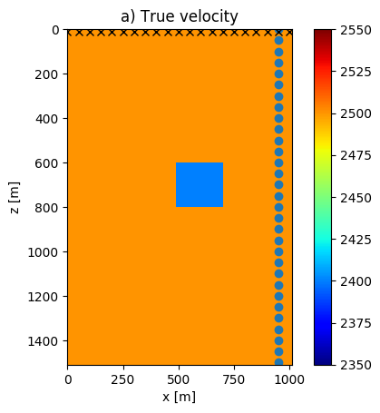
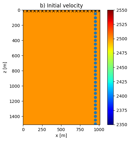
This time, the challenge is to estimate a model (Figure 2a) that has both a background and an anomaly component that are very different from the initial guess (Figure 2b). This means we can no longer fix one of the two components of the generalized Minkowski sum.

The experimental setting is a bit different from the previous example. The sources are in one borehole, the receivers in another borehole at the other side of the model (cross-well full-waveform inversion). Except for a single high-contrast anomaly, the velocity is increasing monotonically, both gradually and discontinuously. The prior knowledge that we assume consists of i) upper and lower bounds on the velocity and also on the anomaly ii) the model is relatively simple in the sense that we assume it has a rank of at most five iii) the background parameters are increasing monotonically with depth iv) the background is varying smoothly in the lateral direction v) the size of the anomaly is not larger than one fifth of the height of the model and not larger than one third of the width of the model. We do not assume prior information on the total-variation of the model, but for comparison, we show the result when we use the true total-variation as a constraint. The following sets formalize the aforementioned prior knowledge:

1. $\mathcal{F}_{1}=\{x\>|\>2350\leq x[i]\leq 2850\}$

2. $\mathcal{F}_{2}=\{x\>|\>\|((D_{z}\otimes I_{x})^{T}\>(I_{z}\otimes D_{x})^{T})^{T}x\|_{1}\leq\sigma\}$

3. $\mathcal{F}_{3}=\{x\>|\>\operatorname{rank}(x)\leq 5\}$

4. $\mathcal{D}_{1}=\{x\>|\>2350\leq x[i]\leq 2850\}$

5. $\mathcal{D}_{2}=\{u\>|\>0\leq(D_{z}\otimes I_{x})u\leq\infty\}$

6. $\mathcal{D}_{3}=\{u\>|\>-0.1\leq(I_{z}\otimes D_{x})u\leq 0.1\}$

7. $\mathcal{E}_{1}=\{v\>|\>300\leq v[i]\leq 350\}$

8. $\mathcal{E}_{2}=\{v\>|\>\operatorname{cardinality}(v)\leq(n_{z}/5\times n_{x}/3)\}$

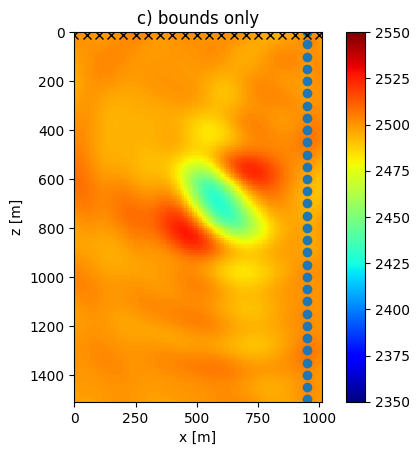
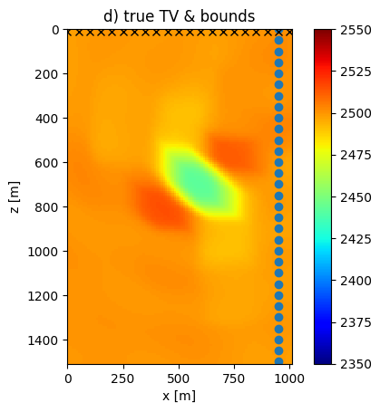
As before, the sets $\mathcal{F}_{k}$ act on the sum of components, $\mathcal{D}_{i}$ describe component one (background), and $\mathcal{E}_{j}$ constrain the other component (anomaly). This collection of prior knowledge is quite specific, but we use it to illustrate how a generalized Minkowski set conveniently includes all this information. Figure 2c shows the model $m$ found by SPG applied to the problem $\min_{m}f(m)\>\>\text{s.t.}\>\>m\in\mathcal{F}_{1}$. We see oscillatory features in the result with bound constraints only, but the main issue is the appearance of a low-velocity artifact, located just below the true anomaly. Figure 2d shows that even if we know the correct total-variation, the result is less oscillatory than using just bound constraints, but still shows an erroneous low-velocity anomaly. When we also include the rank constraint, i.e., we use the set $\mathcal{F}_{1}\bigcap\mathcal{F}_{2}\bigcap\mathcal{F}_{3}$, the result does not improve (Figure 2e). The generalized Minkowski set $\big{(}\bigcap_{k=1}^{3}\mathcal{F}_{k}\big{)}\bigcap\big{(}\bigcap_{i=1}^{3}\mathcal{D}_{i}+\bigcap_{j=1}^{2}\mathcal{E}_{j}\big{)}$ does not yield a result with the large incorrect low-velocity artifact just below the correct high-velocity anomaly (Figure 2g), even though we did not include information on the sign of the anomaly as we did in the previous example. There are still two smaller horizontal and vertical artifacts. Overall, the Minkowski set based constraint results in the best background and anomaly estimation.

(a)

(b)

(c)

(d)

(e)

(f)

Figure 2: The true and initial models corresponding to the full-waveform inversion $2$ example. Figure shows parameter estimation results with various intersections of sets, as well as the result using a generalized Minkowski constraint set. Only the result obtained with the generalized Minkowski set does not show an incorrect low-velocity anomaly.

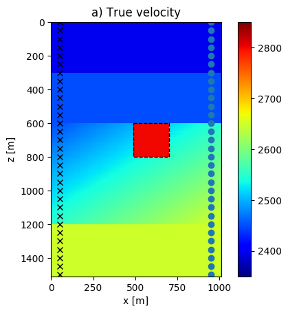
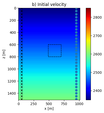
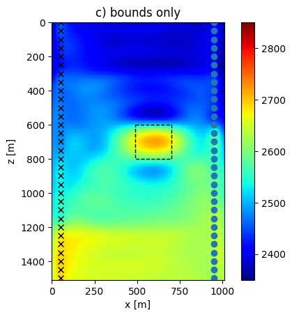
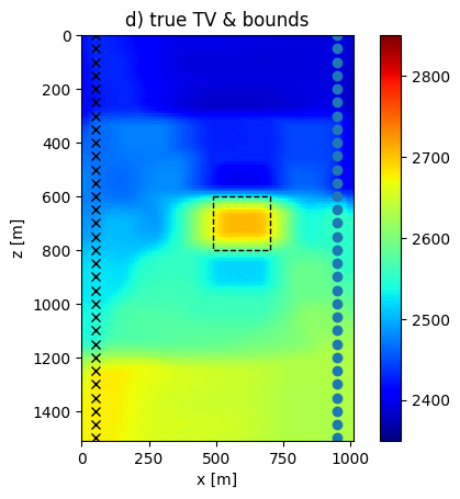
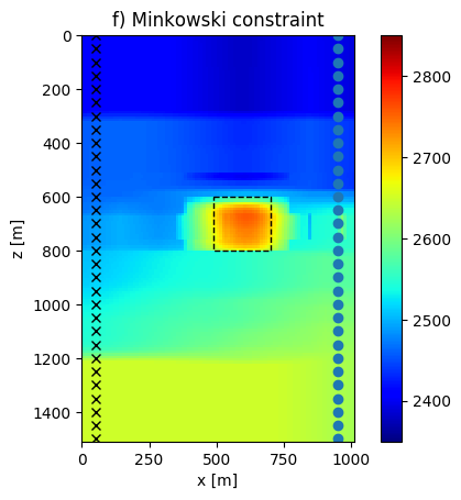
This example shows that the generalized Minkowski set allows for the inclusion of prior knowledge on the two (or more) different components, as well as their sum. The results show that this leads to improved model estimates. Information that we may have about background or anomaly is often difficult or impossible to include in an inverse problem as a single constraint set or intersection of multiple sets, but it fits the summation structure of the generalized Minkowski set. In many practical problems, we do have some information about an anomaly. When looking for air or water filled voids and tunnels in engineering or archeological geophysics, we know that the acoustic wave propagation velocity is usually lower than the background and we also have at least a rough idea about the size of the anomaly. In seismic hydrocarbon exploration, there are high-contrast salt structures in the subsurface, almost always with higher acoustic velocity than the surrounding geology.

5.3 Video processing

Background-anomaly separation of a tensor $T\in\mathbb{R}^{n_{x}\times n_{y}\times n_{t}}$, where $x$ and $y$ are the two spatial coordinates and $t$ is the time, is a common problem in video processing. The separation problem is often used to illustrate robust principal component analysis (RPCA), and related convex and non-convex formulations of sparse + low-rank decomposition algorithms [e.g., Candès et al., 2011, Netrapalli et al., 2014, Kang et al., 2015, Driggs et al., 2017].

Here we show that the generalized Minkowski set for an inverse problem, proposed in Equation (5), describes prior knowledge that is obtained from an example, as well as simple human intuition about a background-anomaly separation problem in video processing. To include multiple pieces of prior knowledge, we choose to work with the video in tensor format and use the flexibility of our regularization framework to impose constraints on the tensor, as well as on individual slices and fibers. This is different from RPCA approaches that matricize or flatten the video tensor to a matrix of size $n_{x}n_{y}\times n_{t}$, such that each column of the matrix is a vectorized time-slice [Candès et al., 2011, Netrapalli et al., 2014, Kang et al., 2015], and also differs from tensor-based RPCA methods that work with a tensor only, e.g., [Zhang et al., 2014, Wang and Navasca, 2015].

Beyond the basic decomposition problem, the escalator video comes with some additional challenges. There is a dynamic background component (the steps of the escalator), and there are reflections of people in the glass that are weak anomalies and duplicates of persons. The video contains noise and part of the background pixel intensity changes significantly ($55$ on a $0-255$ grayscale) over time. We subtract the mean of each time frame as a pre-processing step to mitigate the change in intensity. Below, we describe simple methods to derive prior knowledge for the video background component and how to translate observations and human intuition to a generalized Minkowski set.

Constraint sets for background. We assume that the last $20$ time frames, that do not contain people, are available to derive constraints for the background. From these frames, we use the minimum and maximum value for each pixel over time as the bounds for the background component, denoted as set $\mathcal{D}_{1}$. This is one constraint defined per time fiber. The second constraint is the subspace spanned by the last $20$ frames. We require that each time frame of the background be a linear combination of the training frames organized as a matrix $S\in\mathbb{R}^{n_{x}n_{y}\times 20}$, where each column is a vectorized video frame of $T$. We denote this constraint as $\mathcal{D}_{2}=\{u\>|\>u=Sc,\>c\in\mathbb{R}^{20}\}$, with coefficient vector $c$, which we obtain during the projection operation: $\mathcal{P}_{\mathcal{D}_{2}}(u)=S(S^{T}S)^{-1}S^{T}u$. After computing the singular value decomposition $S=U\Sigma V^{T}$, the projection simplifies to $\mathcal{P}_{\mathcal{D}_{2}}(u)=UU^{T}u$

Constraint sets for sum of components. We constrain the sum of the background and anomaly components to the interval of grayscale values $[0-255]$ minus the mean of each time-frame, denoted as set $\mathcal{F}_{1}$.

Constraint sets for anomaly. There are bound constraints on the anomaly component that we define as the bounds on the sum minus the bounds on the background. We denote this set as $\mathcal{E}_{1}$. To enhance the quality of the anomaly component, we add various types of sparsity constraints. Non-convex sets and set definitions per tensor slice translate simple intuition into constraints. The first type of sparsity constraint is the set $\mathcal{E}_{2}=\{T\>|\>\operatorname{card}(T_{\Omega_{i}})\leq(n_{x}/4\times n_{y}/4)\>\forall i\in\{1,2,\dots,n_{t}\}\}$ where $T_{\Omega_{i}}$ is a time slice of the video tensor. This constraint limits the number of anomaly pixels in each frame to $1/16$ of the total number of pixels in each time slice. The second and third constraint sets are limits on the vertical and horizontal derivative of each time-frame image separately. If we assume the prior knowledge that there are no more than ten persons in the video at each time, we can use $\mathcal{E}_{3}=\{T\>|\>\operatorname{card}((I_{x}\otimes D_{y})\operatorname{vec}(T_{\Omega_{i}}))\leq 480,\>i\in\{1,2,\dots,n_{t}\}\}$, based on the rough estimate of $10\>\text{persons}\times 12\>\text{pixels wide}\times 4\>\text{boundaries}$ (the four vertical boundaries are background - head - upper body - legs - background). Similarly for the horizontal direction, we define $\mathcal{E}_{4}=\{T\>|\>\operatorname{card}((D_{x}\otimes I_{y})\operatorname{vec}(T_{\Omega_{i}}))\leq 440,\>i\in\{1,2,\dots,n_{t}\}\}$.

Putting it all together, we project the video onto the generalized Minkowski set, i.e., we solve

$$\min_{x}\frac{1}{2}\|x-\operatorname{vec}(T)\|_{2}^{2}\>\>\text{s.t.}\>\>x\in\mathcal{F}_{1}\bigcap\big{(}\bigcap_{i=1}^{2}\mathcal{D}_{i}+\bigcap_{j=1}^{4}\mathcal{E}_{j}\big{)}$$ (20)

using the iterations derived in (3). Our formulation implies that the projection of a vector is always the sum of the two components, but this does not mean that $x$ is equal to $T$ at the solution, because we did not include a constraint on $x$ that says we need to fit the data accurately. We did not use a data-fit constraint because it is not evident how tight we want to fit the data or how much noise there is. By computing the projection of the original video, we still include a sense of proximity to the observed data.

Figure 3: Results of the generalized Minkowski decomposition applied to the escalator video. The figure shows four frames. The most noticeable artifacts are in the time stamp.

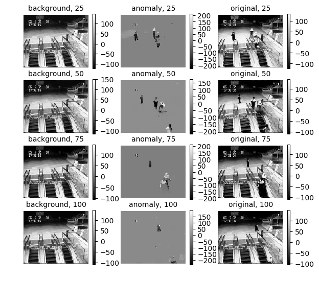
The result of the generalized Minkowski decomposition of the video shown in Figure (3), is visually better than the six methods compared by Driggs et al. [2017]. The compared results often show blurring of the escalator steps in the estimated background, especially when a person is on the escalator. Several results also show visible escalator structure in the anomaly estimation. Our simple approach does not suffer from these two problems. We do not need to estimate any penalty or trade-off parameters but rely on constraint sets based on intuition or whose parameters we can observe directly from a few training frames. We were able to conveniently mix constraints on slices and fibers of the tensor by working with the constrained formulation.

6 Discussion

So far, we described the concepts and algorithms for the case of a Minkowski sum with only two components. Our approach can handle more than two components, but the linear systems in Equation (14) will become larger. A better solver than plain conjugate-gradients can mitigate increased solutions times due to larger linear systems, possibly by taking the block structure into account.

Another potential issue related to Minkowski sums of more than two components is that it will be less intuitive what type of solutions are in the Minkowski sum of sets. We can regain some intuition about the generalized Minkowski set by looking at sampled elements from the set. Samples are simply obtained by projecting vectors (possible solutions, reference models, random vectors, …) onto the target set.

7 Conclusions

Inverse problems for physical parameter estimation and image and video processing often encounter model parameters with complex structure, so that it is difficult to describe the expected model parameters with a single set or intersection of multiple sets. In these situations, it may be easier to work with an additive model description where the model is the sum of morphologically distinct components.

We presented a regularization framework for inverse problems with the Minkowski set at its core. The additive structure of the Minkowski set allows us to enforce prior knowledge in the form of separate constraints on each of the model components. In that sense, our work differs from current approaches that rely on additive penalties for each component. As a result, we no longer need to introduce problematic trade-off parameters.

Unfortunately, the Minkowski set by itself is not versatile enough for physical parameter estimation because we also need to enforce bound constraints and other prior knowledge on the sum of the two components to ensure physical feasibility. Moreover, we would like to use more than one constraint per component to incorporate all prior knowledge that we may have available.

To deal with this situation, we proposed a generalization of the Minkowski set by defining it as the intersection of a Minkowski set with another intersection of constraint sets on the sum of the components. Each of the two or more components of the Minkowski set is also an intersection of sets. With this construction, we can enforce multiple constraints on the model parameters, as well as multiple constraints on each component. The generalized Minkowski set is convex if all contributing sets are convex.

To solve inverse problems with these constraints, we discuss how to project onto generalized Minkowski sets based on the alternating direction method of multipliers. The projection enables projected-gradient based method to minimize nonlinear functions subject to constraints. We also showed that for linear inverse problems, the linear forward operator fits in the projection computation directly as a data-fitting constraint. This makes the inversion faster if the application of the forward operator does not take much time.

Numerical examples show how the generalized Minkowski set helps to solve non-convex seismic parameter estimation problems and a background-anomaly separation task in video processing, given prior knowledge on the model parameters, as well as on the components. The proposed regularization framework thus combines the benefits of constrained problem formulations and additive model descriptions. The algorithms and accompanying software are suitable for toy problems, as well as for larger problems such as videos on 3D grids.

References

- Afonso et al. [2011] M. V. Afonso, J. M. Bioucas-Dias, and M. A. T. Figueiredo. An augmented lagrangian approach to the constrained optimization formulation of imaging inverse problems. IEEE Transactions on Image Processing, 20(3):681–695, March 2011. ISSN 1057-7149. doi: 10.1109/TIP.2010.2076294.
- Barzilai and Borwein [1988] Jonathan Barzilai and Jonathan M. Borwein. Two-point step size gradient methods. IMA Journal of Numerical Analysis, 8(1):141–148, 1988. doi: 10.1093/imanum/8.1.141. URL http://imajna.oxfordjournals.org/content/8/1/141.abstract.
- Beck [2017] A. Beck. First-Order Methods in Optimization. Society for Industrial and Applied Mathematics, Philadelphia, PA, 2017. doi: 10.1137/1.9781611974997. URL http://epubs.siam.org/doi/abs/10.1137/1.9781611974997.
- Bertsekas [1982] Dimitri P. Bertsekas. Projected newton methods for optimization problems with simple constraints. SIAM Journal on Control and Optimization, 20(2):221–246, 1982. doi: 10.1137/0320018. URL https://doi.org/10.1137/0320018.
- Birgin et al. [1999] Ernesto G. Birgin, José Mario Martínez, and Marcos Raydan. Nonmonotone spectral projected gradient methods on convex sets. SIAM J. on Optimization, 10(4):1196–1211, August 1999. ISSN 1052-6234. doi: 10.1137/S1052623497330963. URL http://dx.doi.org/10.1137/S1052623497330963.
- Birgin et al. [2003] Ernesto G. Birgin, José Mario Martínez, and Marcos Raydan. Inexact spectral projected gradient methods on convex sets. IMA Journal of Numerical Analysis, 23(4):539, 2003. doi: 10.1093/imanum/23.4.539. URL +http://dx.doi.org/10.1093/imanum/23.4.539.
- Boyd et al. [2011] Stephen Boyd, Neal Parikh, Eric Chu, Borja Peleato, and Jonathan Eckstein. Distributed optimization and statistical learning via the alternating direction method of multipliers. Found. Trends Mach. Learn., 3(1):1–122, January 2011. ISSN 1935-8237. doi: 10.1561/2200000016. URL http://dx.doi.org/10.1561/2200000016.
- Candès et al. [2011] Emmanuel J. Candès, Xiaodong Li, Yi Ma, and John Wright. Robust principal component analysis? J. ACM, 58(3):11:1–11:37, June 2011. ISSN 0004-5411. doi: 10.1145/1970392.1970395. URL http://doi.acm.org/10.1145/1970392.1970395.
- Combettes [1993] P. L. Combettes. The foundations of set theoretic estimation. Proceedings of the IEEE, 81(2):182–208, Feb 1993. ISSN 0018-9219. doi: 10.1109/5.214546.
- Combettes and Pesquet [2011] Patrick L. Combettes and Jean-Christophe Pesquet. Proximal splitting methods in signal processing. In Heinz H. Bauschke, Regina S. Burachik, Patrick L. Combettes, Veit Elser, D. Russell Luke, and Henry Wolkowicz, editors, Fixed-Point Algorithms for Inverse Problems in Science and Engineering, volume 49 of Springer Optimization and Its Applications, pages 185–212. Springer New York, 2011. ISBN 978-1-4419-9568-1. doi: 10.1007/978-1-4419-9569-8_10. URL http://dx.doi.org/10.1007/978-1-4419-9569-8_10.
- Combettes [1996] P.L. Combettes. The convex feasibility problem in image recovery. volume 95 of Advances in Imaging and Electron Physics, pages 155 – 270. Elsevier, 1996. doi: https://doi.org/10.1016/S1076-5670(08)70157-5. URL http://www.sciencedirect.com/science/article/pii/S1076567008701575.
- Diamond et al. [2018] S. Diamond, R. Takapoui, and S. Boyd. A general system for heuristic minimization of convex functions over non-convex sets. Optimization Methods and Software, 33(1):165–193, 2018. doi: 10.1080/10556788.2017.1304548. URL https://doi.org/10.1080/10556788.2017.1304548.
- Dobkin et al. [1993] David P. Dobkin, John Hershberger, David G. Kirkpatrick, and Subhash Suri. Computing the intersection-depth of polyhedra. Algorithmica, 9:518–533, 1993.
- Driggs et al. [2017] D. Driggs, S. Becker, and A. Aravkin. Adapting Regularized Low Rank Models for Parallel Architectures. ArXiv e-prints, February 2017.
- Eckstein and Yao [2015] Jonathan Eckstein and Wang Yao. Understanding the convergence of the alternating direction method of multipliers: Theoretical and computational perspectives. Pac. J. Optim. To appear, 2015.
- Esser et al. [2018] Ernie Esser, Lluis Guasch, Tristan van Leeuwen, Aleksandr Y. Aravkin, and Felix J. Herrmann. Total variation regularization strategies in full-waveform inversion. SIAM Journal on Imaging Sciences, 11(1):376–406, 2018. doi: 10.1137/17M111328X. URL https://doi.org/10.1137/17M111328X.
- Gao et al. [2011a] Hao Gao, Jian-Feng Cai, Zuowei Shen, and Hongkai Zhao. Robust principal component analysis-based four-dimensional computed tomography. Physics in Medicine and Biology, 56(11):3181, 2011a. URL http://stacks.iop.org/0031-9155/56/i=11/a=002.
- Gao et al. [2011b] Hao Gao, Hengyong Yu, Stanley Osher, and Ge Wang. Multi-energy ct based on a prior rank, intensity and sparsity model (prism). Inverse Problems, 27(11):115012, 2011b. URL http://stacks.iop.org/0266-5611/27/i=11/a=115012.
- Gragnaniello et al. [2012] D. Gragnaniello, C. Chaux, J. C. Pesquet, and L. Duval. A convex variational approach for multiple removal in seismic data. In 2012 Proceedings of the 20th European Signal Processing Conference (EUSIPCO), pages 215–219, Aug 2012.
- Haber et al. [2000] Eldad Haber, Uri M Ascher, and Doug Oldenburg. On optimization techniques for solving nonlinear inverse problems. Inverse Problems, 16(5):1263–1280, October 2000. ISSN 0266-5611. doi: 10.1088/0266-5611/16/5/309. URL http://stacks.iop.org/0266-5611/16/i=5/a=309?key=crossref.98f435f9ee66231b63da02b10f82a60b.
- Hiriart-Urruty and Lemaréchal [2012] Jean-Baptiste Hiriart-Urruty and Claude Lemaréchal. Fundamentals of convex analysis. Springer Science & Business Media, 2012.
- Kang et al. [2015] Z. Kang, C. Peng, and Q. Cheng. Robust pca via nonconvex rank approximation. In 2015 IEEE International Conference on Data Mining, pages 211–220, Nov 2015. doi: 10.1109/ICDM.2015.15.
- Kitic et al. [2016] S. Kitic, L. Albera, N. Bertin, and R. Gribonval. Physics-driven inverse problems made tractable with cosparse regularization. IEEE Transactions on Signal Processing, 64(2):335–348, Jan 2016. ISSN 1053-587X. doi: 10.1109/TSP.2015.2480045.
- Lee et al. [2016] Youngeun Lee, Evan Behar, Jyh-Ming Lien, and Young J. Kim. Continuous penetration depth computation for rigid models using dynamic minkowski sums. Computer-Aided Design, 78:14 – 25, 2016. ISSN 0010-4485. doi: https://doi.org/10.1016/j.cad.2016.05.012. URL http://www.sciencedirect.com/science/article/pii/S001044851630032X. SPM 2016.
- Meyer [2001] Yves Meyer. Oscillating patterns in image processing and nonlinear evolution equations: the fifteenth Dean Jacqueline B. Lewis memorial lectures, volume 22. American Mathematical Soc., 2001.
- Netrapalli et al. [2014] Praneeth Netrapalli, Niranjan U N, Sujay Sanghavi, Animashree Anandkumar, and Prateek Jain. Non-convex robust pca. In Z. Ghahramani, M. Welling, C. Cortes, N. D. Lawrence, and K. Q. Weinberger, editors, Advances in Neural Information Processing Systems 27, pages 1107–1115. Curran Associates, Inc., 2014. URL http://papers.nips.cc/paper/5430-non-convex-robust-pca.pdf.
- Nocedal and Wright [2000] J Nocedal and S J Wright. Numerical optimization. Springer, 2000.
- Ono et al. [2014] S. Ono, T. Miyata, and I. Yamada. Cartoon-texture image decomposition using blockwise low-rank texture characterization. IEEE Transactions on Image Processing, 23(3):1128–1142, March 2014. ISSN 1057-7149. doi: 10.1109/TIP.2014.2299067.
- Osher et al. [2003] Stanley Osher, Andrés Solé, and Luminita Vese. Image decomposition and restoration using total variation minimization and the h1. Multiscale Modeling and Simulation, 1(3):349–370, 2003. doi: 10.1137/S1540345902416247. URL http://dx.doi.org/10.1137/S1540345902416247.
- Paige and Saunders [1982] Christopher C. Paige and Michael A. Saunders. Lsqr: An algorithm for sparse linear equations and sparse least squares. ACM Trans. Math. Softw., 8(1):43–71, March 1982. ISSN 0098-3500. doi: 10.1145/355984.355989. URL http://doi.acm.org/10.1145/355984.355989.
- Parikh and Boyd [2014] Neal Parikh and Stephen Boyd. Proximal algorithms. Foundations and Trends® in Optimization, 1(3):127–239, 2014. ISSN 2167-3888. doi: 10.1561/2400000003. URL http://dx.doi.org/10.1561/2400000003.
- Peters and Herrmann [2017] Bas Peters and Felix J. Herrmann. Constraints versus penalties for edge-preserving full-waveform inversion. The Leading Edge, 36(1):94–100, 2017. doi: 10.1190/tle36010094.1. URL http://dx.doi.org/10.1190/tle36010094.1.
- Peters and Herrmann [2019] Bas Peters and Felix J Herrmann. Algorithms and software for projections onto intersections of convex and non-convex sets with applications to inverse problems. arXiv preprint arXiv:1902.09699, 2019.
- Peters et al. [2018] Bas Peters, Brendan R. Smithyman, and Felix J. Herrmann. Projection methods and applications for seismic nonlinear inverse problems with multiple constraints. GEOPHYSICS, 0(ja):1–100, 2018. doi: 10.1190/geo2018-0192.1. URL https://doi.org/10.1190/geo2018-0192.1.
- Pham et al. [2014a] M. Q. Pham, C. Chaux, L. Duval, and J. C. Pesquet. A constrained-based optimization approach for seismic data recovery problems. In 2014 IEEE International Conference on Acoustics, Speech and Signal Processing (ICASSP), pages 2377–2381, May 2014a. doi: 10.1109/ICASSP.2014.6854025.
- Pham et al. [2014b] M. Q. Pham, L. Duval, C. Chaux, and J. C. Pesquet. A primal-dual proximal algorithm for sparse template-based adaptive filtering: Application to seismic multiple removal. IEEE Transactions on Signal Processing, 62(16):4256–4269, Aug 2014b. ISSN 1053-587X. doi: 10.1109/TSP.2014.2331614.
- Pratt et al. [1998] G.R. Pratt, Changsoo Shin, and G.J. Hicks. Gauss-Newton and full Newton methods in frequency-space seismic waveform inversion. Geophysical Journal International, 133(2):341–362, May 1998. ISSN 0956540X. doi: 10.1046/j.1365-246X.1998.00498.x. URL http://doi.wiley.com/10.1046/j.1365-246X.1998.00498.x.
- Schaeffer and Osher [2013] Hayden Schaeffer and Stanley Osher. A low patch-rank interpretation of texture. SIAM Journal on Imaging Sciences, 6(1):226–262, 2013. doi: 10.1137/110854989. URL http://dx.doi.org/10.1137/110854989.
- Schmidt et al. [2009] Mark Schmidt, Ewout Van Den Berg, Michael P Friedlander, and Kevin Murphy. Optimizing costly functions with simple constraints: A limited-memory projected quasi-newton algorithm. In Proc. of Conf. on Artificial Intelligence and Statistics, 2009.
- Schmidt et al. [2012] Mark Schmidt, Dongmin Kim, and Suvrit Sra. Projected Newton-type Methods in Machine Learning, volume 35, chapter 11, pages 305–327. MIT Press, 04 2012.
- Smithyman et al. [2015] BR Smithyman, B Peters, and FJ Herrmann. Constrained waveform inversion of colocated vsp and surface seismic data. In 77th EAGE Conference and Exhibition 2015, 2015.
- Song et al. [2016] Changkyu Song, Sejong Yoon, and Vladimir Pavlovic. Fast admm algorithm for distributed optimization with adaptive penalty. In Proceedings of the Thirtieth AAAI Conference on Artificial Intelligence, AAAI’16, pages 753–759. AAAI Press, 2016. URL http://dl.acm.org/citation.cfm?id=3015812.3015924.
- Starck et al. [2005] J. L. Starck, M. Elad, and D. L. Donoho. Image decomposition via the combination of sparse representations and a variational approach. IEEE Transactions on Image Processing, 14(10):1570–1582, Oct 2005. ISSN 1057-7149. doi: 10.1109/TIP.2005.852206.
- Tadmor et al. [2004] E. Tadmor, S. Nezzar, and L. Vese. A multiscale image representation using hierarchical (bv,l2 ) decompositions. Multiscale Modeling & Simulation, 2(4):554–579, 2004. doi: 10.1137/030600448. URL https://doi.org/10.1137/030600448.
- Tarantola [1986] A. Tarantola. A strategy for nonlinear elastic inversion of seismic reflection data. GEOPHYSICS, 51(10):1893–1903, 1986. doi: 10.1190/1.1442046. URL http://library.seg.org/doi/abs/10.1190/1.1442046.
- Trussell and Civanlar [1984] H. Trussell and M. Civanlar. The feasible solution in signal restoration. IEEE Transactions on Acoustics, Speech, and Signal Processing, 32(2):201–212, April 1984. ISSN 0096-3518. doi: 10.1109/TASSP.1984.1164297.
- Varadhan and Manocha [2006] Gokul Varadhan and Dinesh Manocha. Accurate minkowski sum approximation of polyhedral models. Graphical Models, 68(4):343 – 355, 2006. ISSN 1524-0703. doi: https://doi.org/10.1016/j.gmod.2005.11.003. URL http://www.sciencedirect.com/science/article/pii/S1524070306000191. PG2004.
- Virieux and Operto [2009] J Virieux and S Operto. An overview of full-waveform inversion in exploration geophysics. Geophysics, 74(6):WCC1–WCC26, 2009. URL http://dx.doi.org/10.1190/1.3238367.
- Wang and Navasca [2015] Xiaofei Wang and Carmeliza Navasca. Adaptive low rank approximation for tensors. In The IEEE International Conference on Computer Vision (ICCV) Workshops, December 2015.
- Xu et al. [2016] Zheng Xu, Soham De, Mario Figueiredo, Christoph Studer, and Tom Goldstein. An empirical study of admm for nonconvex problems. In NIPS workshop on nonconvex optimization, 2016.
- Xu et al. [2017a] Zheng Xu, Mario Figueiredo, and Tom Goldstein. Adaptive ADMM with Spectral Penalty Parameter Selection. In Aarti Singh and Jerry Zhu, editors, Proceedings of the 20th International Conference on Artificial Intelligence and Statistics, volume 54 of Proceedings of Machine Learning Research, pages 718–727, Fort Lauderdale, FL, USA, 20–22 Apr 2017a. PMLR. URL http://proceedings.mlr.press/v54/xu17a.html.
- Xu et al. [2017b] Zheng Xu, Mario A. T. Figueiredo, Xiaoming Yuan, Christoph Studer, and Tom Goldstein. Adaptive relaxed admm: Convergence theory and practical implementation. In The IEEE Conference on Computer Vision and Pattern Recognition (CVPR), July 2017b.
- Xu et al. [2017c] Zheng Xu, Gavin Taylor, Hao Li, Mário A. T. Figueiredo, Xiaoming Yuan, and Tom Goldstein. Adaptive consensus ADMM for distributed optimization. In Doina Precup and Yee Whye Teh, editors, Proceedings of the 34th International Conference on Machine Learning, volume 70 of Proceedings of Machine Learning Research, pages 3841–3850, International Convention Centre, Sydney, Australia, 06–11 Aug 2017c. PMLR. URL http://proceedings.mlr.press/v70/xu17c.html.
- Yong et al. [2018] Peng Yong, Wenyuan Liao, Jianping Huang, and Zhenchuan Li. Total variation regularization for seismic waveform inversion using an adaptive primal dual hybrid gradient method. Inverse Problems, 34(4):045006, 2018. URL http://stacks.iop.org/0266-5611/34/i=4/a=045006.
- Youla and Webb [1982] D. C. Youla and H. Webb. Image restoration by the method of convex projections: Part 1-theory. IEEE Transactions on Medical Imaging, 1(2):81–94, Oct 1982. ISSN 0278-0062. doi: 10.1109/TMI.1982.4307555.
- Zhang et al. [2014] Zemin Zhang, Gregory Ely, Shuchin Aeron, Ning Hao, and Misha Kilmer. Novel methods for multilinear data completion and de-noising based on tensor-svd. In The IEEE Conference on Computer Vision and Pattern Recognition (CVPR), June 2014.