Asynchronous Federated Optimization

Abstract

Federated learning enables training on a massive number of edge devices. To improve flexibility and scalability, we propose a new asynchronous federated optimization algorithm. We prove that the proposed approach has near-linear convergence to a global optimum, for both strongly convex and a restricted family of non-convex problems. Empirical results show that the proposed algorithm converges quickly and tolerates staleness in various applications.

1 Introduction

Federated learning [Konevcnỳ et al.(2016)Konevcnỳ, McMahan, Yu, Richtárik, Suresh, and Bacon, McMahan et al.(2016)McMahan, Moore, Ramage, Hampson, et al.] enables training a global model on datasets partitioned across a massive number of resource-weak edge devices. Motivated by the modern phenomenon of distributed (often personal) data collected by edge devices at scale, federated learning can use the large amounts of training data from diverse users for better representation and generalization. Federated learning is also motivated by the desire for privacy preservation [Bonawitz et al.(2019)Bonawitz, Eichner, Grieskamp, Huba, Ingerman, Ivanov, Kiddon, Konecny, Mazzocchi, McMahan, et al., Bonawitz et al.(2017)Bonawitz, Ivanov, Kreuter, Marcedone, McMahan, Patel, Ramage, Segal, and Seth]. In some scenarios, on-device training without depositing data in the cloud may be legally required by regulations [Steve Anderson: HealthInsurance.org(1996), US Department of Education(2019), EU(2018)].

A federated learning system is often composed of servers and workers, with an architecture that is similar to parameter servers [Li et al.(2014a)Li, Andersen, Park, Smola, Ahmed, Josifovski, Long, Shekita, and Su, Li et al.(2014b)Li, Andersen, Smola, and Yu, Ho et al.(2013)Ho, Cipar, Cui, Lee, Kim, Gibbons, Gibson, Ganger, and Xing]. The workers (edge devices) train the models locally on private data. The servers aggregate the learned models from the workers and update the global model.

Federated learning has three key properties [Konevcnỳ et al.(2016)Konevcnỳ, McMahan, Yu, Richtárik, Suresh, and Bacon, McMahan et al.(2016)McMahan, Moore, Ramage, Hampson, et al.]: 1) Infrequent task activation. For the weak edge devices, learning tasks are executed only when the devices are idle, charging, and connected to unmetered networks [Bonawitz et al.(2019)Bonawitz, Eichner, Grieskamp, Huba, Ingerman, Ivanov, Kiddon, Konecny, Mazzocchi, McMahan, et al.]. 2) Infrequent communication. The connection between edge devices and the remote servers may frequently be unavailable, slow, or expensive (in terms of communication costs or battery power usage). 3) Non-IID training data. For federated learning, the data on different devices are disjoint, thus may represent non-identically distributed samples from the population.

Federated learning [McMahan et al.(2016)McMahan, Moore, Ramage, Hampson, et al., Bonawitz et al.(2019)Bonawitz, Eichner, Grieskamp, Huba, Ingerman, Ivanov, Kiddon, Konecny, Mazzocchi, McMahan, et al.] is most often implemented using the synchronous approach, which could be slow due to stragglers. When handling massive edge devices, there could be a large number of stragglers. As availability and completion time vary from device to device, due to limited computational capacity and battery time, the global synchronization is difficult, especially in the federated learning scenario.

Asynchronous training [Zinkevich et al.(2009)Zinkevich, Langford, and Smola, Lian et al.(2017)Lian, Zhang, Zhang, and Liu, Zheng et al.(2017)Zheng, Meng, Wang, Chen, Yu, Ma, and Liu] is widely used in traditional distributed stochastic gradient descent (SGD) for stragglers and heterogeneous latency  [Zinkevich et al.(2009)Zinkevich, Langford, and Smola, Lian et al.(2017)Lian, Zhang, Zhang, and Liu, Zheng et al.(2017)Zheng, Meng, Wang, Chen, Yu, Ma, and Liu]. In this paper, we take the advantage of asynchronous training and combines it with federated optimization.

We propose a novel asynchronous algorithm for federated optimization. The key ideas are (i) to solve regularized local problems to guarantee convergence, and (ii) then use a weighted average to update the global model, where the mixing weight is set adaptively as a function of the staleness. Together, these techniques result in an effective asynchronous federated optimization procedure. The main contributions of our paper are listed as follows:

• We propose a new asynchronous federated optimization algorithm and a prototype system design.

• We prove the convergence of the proposed approach for a restricted family of non-convex problems.

• We propose strategies for controlling the error caused by asynchrony. To this end, we introduce a mixing hyperparameter which adaptively controls the trade-off between the convergence rate and variance reduction according to the staleness.

• We show empirically that the proposed algorithm converges quickly and often outperforms synchronous federated optimization in practical settings.

Table 1: Notations and Terminologies.

Notation	Description
$n$	Number of devices
$T$	Number of global epochs
$[n]$	Set of integers $\{1,\ldots,n\}$
$H_{min}$	Minimal number of local iterations
$H_{max}$	Maximal number of local iterations
$\delta$	$\delta=\frac{H_{max}}{H_{min}}$ is the imbalance ratio
$H^{i}_{\tau}$	Number of local iterations
	in the $\tau^{\mbox{th}}$ epoch on the $i$th device
$x_{t}$	Global model in the $t^{\mbox{th}}$ epoch on server
$x^{i}_{\tau,h}$	Model initialized from $x_{\tau}$, updated in
	the $h$th local iteration, on the $i$th device
$\mathcal{D}^{i}$	Dataset on the $i$th device
$z^{i}_{t,h}$	Data (minibatch) sampled from $\mathcal{D}^{i}$
$\gamma$	Learning rate
$\alpha$	Mixing hyperparameter
$\rho$	Regularization weight
$t-\tau$	Staleness
$s(t-\tau)$	Function of staleness for adaptive $\alpha$
$\|\cdot\|$	All the norms in this paper are $l_{2}$-norms
Device	Where the training data are placed
Worker	One worker on each device,
	process that trains the model

Figure 1: System overview. \small0⃝: scheduler triggers training through coordinator. \small1⃝, \small2⃝: worker receives model $x_{t-\tau}$ from server via coordinator. \small3⃝: worker computes local updates as Algorithm 1. Worker can switch between the two states: working and idle. \small4⃝, \small5⃝, \small6⃝: worker pushes the locally updated model to server via the coordinator. Coordinator queues the models received in \small5⃝, and feeds them to the updater sequentially in \small6⃝. \small7⃝, \small8⃝: server updates the global model and makes it ready to read in the coordinator. In our system, \small1⃝ and \small5⃝ operate asynchronously in parallel.

2 Problem formulation

We consider federated learning with $n$ devices. On each device, a worker process trains a model on local data. The overall goal is to train a global model $x\in{\mathbb{R}}^{d}$ using data from all the devices. Formally, we solve $\min_{x\in{\mathbb{R}}^{d}}F(x),$ where $F(x)=\frac{1}{n}\sum_{i\in[n]}{\mathbb{E}}_{z^{i}\sim\mathcal{D}^{i}}f(x;z^{i})$, for $\forall i\in[n]$, $z^{i}$ is sampled from the local data $\mathcal{D}^{i}$ on the $i$th device. Note that different devices have different local datasets, i.e., $\mathcal{D}^{i}\neq\mathcal{D}^{j},\forall i\neq j$.

3 Methodology

The training takes $T$ global epochs. In the $t^{\mbox{th}}$ epoch, the server receives a locally trained model $x_{new}$ from an arbitrary worker, and updates the global model by weighted averaging: $x_{t}=(1-\alpha)x_{t-1}+\alpha x_{new},$ where $\alpha\in(0,1)$ is the mixing hyperparameter. A system overview is illustrated in Figure 1.

On an arbitrary device $i$, after receiving a global model $x_{t}$ (potentially stale) from the server, we locally solve the following regularized optimization problem using SGD for multiple iterations: $\min_{x\in{\mathbb{R}}^{d}}{\mathbb{E}}_{z^{i}\sim\mathcal{D}^{i}}f(x;z^{i})+\frac{\rho}{2}\|x-x_{t}\|^{2}.$ For convenience, we define $g_{x^{\prime}}(x;z)=f(x;z)+\frac{\rho}{2}\|x-x^{\prime}\|^{2}$.

Algorithm 1 Asynchronous Federated Optimization (FedAsync)

FServerServer FSchedulerScheduler FUpdaterUpdater FWorkerWorker

FnProcess: $\alpha\in(0,1)$ Initialize $x_{0}$, $\alpha_{t}\leftarrow\alpha,\forall t\in[T]$
Run Scheduler() thread and Updater() thread asynchronously in parallel

FnThread: Periodically trigger training tasks on some workers, and send the global model with time stamp

FnThread:

for epoch $t\in[T]$ do Receive the pair $(x_{new},\tau)$ from any worker
Optional: $\alpha_{t}\leftarrow\alpha\times s(t-\tau)$, $s(\cdot)$ is a function of the staleness
$x_{t}\leftarrow(1-\alpha_{t})x_{t-1}+\alpha_{t}x_{new}$

FnProcess:

for $i\in[n]$ in parallel do

if triggered by the scheduler then Receive the pair of the global model and its time stamp $(x_{t},t)$ from the server
$\tau\leftarrow t$, $x_{\tau,0}^{i}\leftarrow x_{t}$
Define $g_{x_{t}}(x;z)=f(x;z)+\frac{\rho}{2}\|x-x_{t}\|^{2}$, where $\rho>\mu$

for local iteration $h\in[H_{\tau}^{i}]$ do Randomly sample $z_{\tau,h}^{i}\sim\mathcal{D}^{i}$
Update $x_{\tau,h}^{i}\leftarrow x_{\tau,h-1}^{i}-\gamma\nabla g_{x_{t}}(x_{\tau,h-1}^{i};z_{\tau,h}^{i})$ Push $(x_{\tau,H_{\tau}^{i}}^{i},\tau)$ to the server

The server and workers conduct updates asynchronously, i.e., the server immediately updates the global model whenever it receives a local model. The communication between the server and the workers is non-blocking. Thus, the server and workers can update the models at any time without synchronization, which is favorable when the devices have heterogeneous conditions.

The detailed algorithm is shown in Algorithm 1. The model parameter $x_{\tau,h}^{i}$ is updated in the $h$th local iteration after receiving $x_{\tau}$, on the $i$th device. The data $z_{\tau,h}^{i}$ is randomly drawn in the $h$th local iteration after receiving $x_{\tau}$, on the $i$th device. $H_{\tau}^{i}$ is the number of local iterations after receiving $x_{\tau}$ on the $i$th device. $\gamma$ is the learning rate and $T$ is the total number of global epochs.

Remark 3.1.

On the server side, the scheduler and the updater run asynchronously in parallel. The scheduler periodically triggers training tasks and controls the staleness ($t-\tau$ in the updater thread). The updater receives models from workers and updates the global model. Our architecture allows for multiple updater threads with read-write lock on the global model, which improves the throughput.

Remark 3.2.

Intuitively, larger staleness results in greater error when updating the global model. For the local models with large staleness $(t-\tau)$, we can decrease $\alpha$ to mitigate the error caused by staleness. As shown in Algorithm 1, optionally, we use a function $s(t-\tau)$ to determine the value of $\alpha$. In general, $s(t-\tau)$ should be $1$ when $t=\tau$, and monotonically decrease when $(t-\tau)$ increases. There are many functions that satisfy such two properties, with different decreasing rate, e.g., $s_{a}(t-\tau)=\frac{1}{t-\tau+1}$. The options used in this paper can be found in Section 5.2.

4 Convergence analysis

First, we introduce some definitions and assumptions for our convergence analysis.

Definition 4.1.

(Smoothness) A differentiable function $f$ is $L$-smooth if for $\forall x,y$, $f(y)-f(x)\leq\left\langle\nabla f(x),y-x\right\rangle+\frac{L}{2}\|y-x\|^{2},$ where $L>0$.

Definition 4.2.

(Weak convexity) A differentiable function $f$ is $\mu$-weakly convex if the function $g$ with $g(x)=f(x)+\frac{\mu}{2}\|x\|^{2}$ is convex, where $\mu\geq 0$. $f$ is convex if $\mu=0$, and non-convex if $\mu>0$.

We have the following convergence guarantees. Detailed proofs can be found in the appendix.

Theorem 4.3.

Assume that $F$ is $L$-smooth and $\mu$-weakly convex, and each worker executes at least $H_{min}$ and at most $H_{max}$ local updates before pushing models to the server. We assume bounded delay $t-\tau\leq K$. The imbalance ratio of local updates is $\delta=\frac{H_{max}}{H_{min}}$. Furthermore, we assume that for $\forall x\in{\mathbb{R}}^{d},i\in[n]$, and $\forall z\sim\mathcal{D}^{i}$, we have $\|\nabla f(x;z)\|^{2}\leq V_{1}$ and $\|\nabla g_{x^{\prime}}(x;z)\|^{2}\leq V_{2}$, $\forall x^{\prime}$. For any small constant $\epsilon>0$, taking $\rho$ large enough such that $\rho>\mu$ and $-(1+2\rho+\epsilon)V_{2}+\rho^{2}\|x_{\tau,h-1}-x_{\tau}\|^{2}-\frac{\rho}{2}\|x_{\tau,h-1}-x_{\tau}\|^{2}\geq 0,\forall x_{\tau,h-1},x_{\tau}$, and $\gamma<\frac{1}{L}$, after $T$ global updates, Algorithm 1 converges to a critical point: $\min_{t=0}^{T-1}{\mathbb{E}}\|\nabla F(x_{t})\|^{2}\leq\frac{{\mathbb{E}}\left[F(x_{0})-F(x_{T})\right]}{\alpha\gamma\epsilon TH_{min}}+{\mathcal{O}}\left(\frac{\gamma H_{max}^{3}+\alpha KH_{max}}{\epsilon H_{min}}\right)+{\mathcal{O}}\left(\frac{\alpha^{2}\gamma K^{2}H_{max}^{2}+\gamma K^{2}H_{max}^{2}}{\epsilon H_{min}}\right).$

5 Experiments

In this section, we empirically evaluate the proposed algorithm.

5.1 Datasets

We conduct experiments on two benchmarks: CIFAR-10 [Krizhevsky and Hinton(2009)], and WikiText-2 [Merity et al.(2016)Merity, Xiong, Bradbury, and Socher]. The training set is partitioned onto $n=100$ devices. The mini-batch sizes are 50 and 20 respectively.

5.2 Evaluation setup

The baseline algorithm is FedAvg introduced by [McMahan et al.(2016)McMahan, Moore, Ramage, Hampson, et al.], which implements synchronous federated optimization. For FedAvg, in each epoch, $k=10$ devices are randomly selected to launch local updates. We also consider single-thread SGD as a baseline. For FedAsync, we simulate the asynchrony by randomly sampling the staleness $(t-\tau)$ from a uniform distribution.

We repeat each experiment 10 times and take the average. For CIFAR-10, we use the top-1 accuracy on the testing set as the evaluation metric. To compare asynchronous training and synchronous training, we consider “metrics vs. number of gradients”. The “number of gradients” is the number of gradients applied to the global model.

For convenience, we name Algorithm 1 as FedAsync. We also test the performance of FedAsync with adaptive mixing hyperparameters $\alpha_{t}=\alpha\times s(t-\tau)$, as outlined in Section 3. We employ the following three strategies for the weighting function $s(t-\tau)$ (parameterized by $a,b>0$): • Constant: $s(t-\tau)=1$. • Polynomial: $s_{a}(t-\tau)=(t-\tau+1)^{-a}$. • Hinge: $s_{a,b}(t-\tau)=\begin{cases}1&\mbox{if $t-\tau\leq b$}\\ \frac{1}{a(t-\tau-b)+1}&\mbox{otherwise}\end{cases}.$

For convenience, we refer to FedAsync with constant $\alpha$ as FedAsync+Const, FedAsync with polynomial adaptive $\alpha$ as FedAsync+Poly, and FedAsync with hinge adaptive $\alpha$ as FedAsync+Hinge.

[Top-1 accuracy on testing set, $t-\tau\leq 4$] [Top-1 accuracy on testing set, $t-\tau\leq 16$]

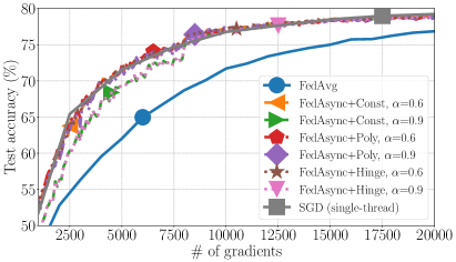
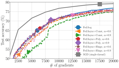
Figure 2: Top-1 accuracy (the higher the better) vs. # of gradients on CNN and CIFAR-10 dataset. The maximum staleness is $4$ or $16$. $\gamma=0.1$, $\rho=0.005$. For FedAsync+Poly, we take $a=0.5$. For FedAsync+Hinge, we take $a=10,b=4$. Note that when the maximum staleness is $4$, FedAsync+Const and FedAsync+Hinge with $b=4$ are the same.

5.3 Empirical results

We test FedAsync (asynchronous federated optimization in Algorithm 1) with different learning rates $\gamma$, regularization weights $\rho$, mixing hyperparameter $\alpha$, and staleness.

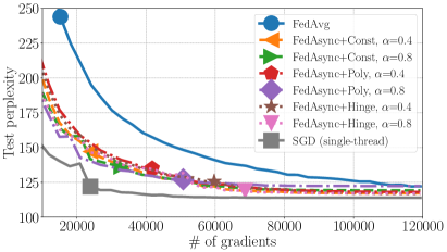
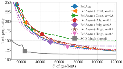
In Figure 2 and 3, we show how FedAsync converges when the number of gradients grows. We can see that when the overall staleness is small, FedAsync converges as fast as SGD, and faster than FedAvg. When the staleness is larger, FedAsync converges slower. In the worst case, FedAsync has similar convergence rate as FedAvg. When $\alpha$ is too large, the convergence can be unstable, especially for FedAsync+Const. The convergence is more robust when adaptive $\alpha$ is used.

[Perplexity on testing set, $t-\tau\leq 4$] [Perplexity on testing set, $t-\tau\leq 16$]

Figure 3: Perplexity (the lower the better) vs. # of gradients on LSTM-based language model and WikiText-2 dataset. The maximum staleness is $4$ or $16$. $\gamma=20$, $\rho=0.0001$. For FedAsync+Poly, we take $a=0.5$. For FedAsync+Hinge, we take $a=10,b=2$.

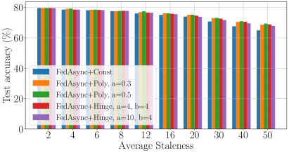
In Figure 4, we show how staleness affects the convergence of FedAsync, evaluated on CNN and CIFAR-10 dataset. Overall, larger staleness makes the convergence slower, but the influence is not catastrophic. Furthermore, the instability caused by large staleness can be mitigated by using adaptive $\alpha$. Using adaptive $\alpha$ always improves the performance, compared to using constant $\alpha$.

Figure 4: Top-1 accuracy on CNN and CIFAR-10 dataset at the end of training, with different staleness. $\gamma=0.1$, $\rho=0.01$. $\alpha$ has initial value $0.9$.

5.4 Discussion

In general, the convergence rate of FedAsync is between single-thread SGD and FedAvg. Larger $\alpha$ and smaller staleness make FedAsync closer to single-thread SGD. Smaller $\alpha$ and larger staleness makes FedAsync closer to FedAvg.

Empirically, we observe that FedAsync is generally insensitive to hyperparameters. When the staleness is large, we can tune $\alpha$ to improve the convergence. Without adaptive $\alpha$, smaller $\alpha$ is better for larger staleness. For adaptive $\alpha$, our best choice empirically was FedAsync+Hinge. FedAsync+Poly and FedAsync+Hinge have similar performance.

In summary, compared to FedAvg, FedAsync performs as good as, and in most cases better. When the staleness is small, FedAsync converges much faster than FedAvg. When the staleness is large, FedAsync still achieves similar performance as FedAvg.

6 Conclusion

We proposed a novel asynchronous federated optimization algorithm on non-IID training data. We proved the convergence for a restricted family of non-convex problems. Our empirical evaluation validated both fast convergence and staleness tolerance. An interesting future direction is the design of strategies to adaptively tune the mixing hyperparameters.

This work was funded in part by the following grants: NSF IIS 1909577, NSF CNS 1908888, NSF CCF 1934986 and a JP Morgan Chase Fellowship, along with computational resources donated by Intel, AWS, and Microsoft Azure.

Appendix

Appendix A Proofs

Theorem A.1.

Assume that $F$ is $L$-smooth and $\mu$-weakly convex, and each worker executes at least $H_{min}$ and at most $H_{max}$ local updates before pushing models to the server. We assume bounded delay $t-\tau\leq K$. The imbalance ratio of local updates is $\delta=\frac{H_{max}}{H_{min}}$. Furthermore, we assume that for $\forall x\in{\mathbb{R}}^{d},i\in[n]$, and $\forall z\sim\mathcal{D}^{i}$, we have $\|\nabla f(x;z)\|^{2}\leq V_{1}$ and $\|\nabla g_{x^{\prime}}(x;z)\|^{2}\leq V_{2}$, $\forall x^{\prime}$. Taking $\rho$ large enough such that $\rho>\mu$ and $-(1+2\rho+\epsilon)V_{2}+\rho^{2}\|x_{\tau,h-1}-x_{\tau}\|^{2}-\frac{\rho}{2}\|x_{\tau,h-1}-x_{\tau}\|^{2}\geq 0,\forall x_{\tau,h-1},x_{\tau}$, and $\gamma<\frac{1}{L}$, after $T$ global updates, Algorithm 1 converges to a critical point:

$$\min_{t=0}^{T-1}{\mathbb{E}}\|\nabla F(x_{t})\|^{2}$$

$$\leq\frac{{\mathbb{E}}\left[F(x_{0})-F(x_{T})\right]}{\alpha\gamma\epsilon TH_{min}}+{\mathcal{O}}\left(\frac{\gamma H_{max}^{3}+\alpha KH_{max}+\alpha^{2}\gamma K^{2}H_{max}^{2}+\gamma K^{2}H_{max}^{2}}{\epsilon H_{min}}\right).$$

Taking $\alpha=\frac{1}{\sqrt{H_{min}}}$, $\gamma=\frac{1}{\sqrt{T}}$, $T=H_{min}^{5}$, we have

$$\min_{t=0}^{T-1}{\mathbb{E}}\|\nabla F(x_{t})\|^{2}\leq{\mathcal{O}}\left(\frac{1}{\epsilon H_{min}^{3}}+\frac{\delta^{3}}{\epsilon\sqrt{H_{min}}}+\frac{K\delta}{\epsilon\sqrt{H_{min}}}+\frac{K^{2}\delta^{2}}{\epsilon\sqrt{H_{min}^{5}}}+\frac{K^{2}\delta^{2}}{\epsilon\sqrt{H_{min}^{3}}}\right).$$

Proof A.2.

Without loss of generality, we assume that in the $t^{\mbox{th}}$ epoch, the server receives the model $x_{new}$, with time stamp $\tau$. We assume that $x_{new}$ is the result of applying $H_{min}\leq H\leq H_{max}$ local updates to $x_{\tau}$ on the $i$th device. We also ignore $i$ in $x_{\tau,h}^{i}$ and $z_{\tau,h}^{i}$ for convenience.

Thus, using smoothness and strong convexity, conditional on $x_{\tau,h-1}$, for $\forall h\in[H]$ we have

$${\mathbb{E}}\left[F(x_{\tau,h})-F(x_{*})\right]$$

$$\leq{\mathbb{E}}\left[G_{x_{\tau}}(x_{\tau,h})-F(x_{*})\right]$$

$$\leq G_{x_{\tau}}(x_{\tau,h-1})-F(x_{*})-\gamma{\mathbb{E}}\left[\left\langle\nabla G_{x_{\tau}}(x_{\tau,h-1}),\nabla g_{x_{\tau}}(x_{\tau,h-1};z_{\tau,h})\right\rangle\right]$$

$$\quad+\frac{L\gamma^{2}}{2}{\mathbb{E}}\left[\|\nabla g_{x_{\tau}}(x_{\tau,h-1};z_{\tau,h})\|^{2}\right]$$

$$\leq F(x_{\tau,h-1})-F(x_{*})+\frac{\rho}{2}\|x_{\tau,h-1}-x_{\tau}\|^{2}-\gamma{\mathbb{E}}\left[\left\langle\nabla G_{x_{\tau}}(x_{\tau,h-1}),\nabla g_{x_{\tau}}(x_{\tau,h-1};z_{\tau,h})\right\rangle\right]$$

$$\quad+\frac{L\gamma^{2}}{2}{\mathbb{E}}\left[\|\nabla g_{x_{\tau}}(x_{\tau,h-1};z_{\tau,h})\|^{2}\right]$$

$$\leq F(x_{\tau,h-1})-F(x_{*})-\gamma{\mathbb{E}}\left[\left\langle\nabla G_{x_{\tau}}(x_{\tau,h-1}),\nabla g_{x_{\tau}}(x_{\tau,h-1};z_{\tau,h})\right\rangle\right]+\frac{L\gamma^{2}}{2}V_{2}+\frac{\rho H_{max}^{2}\gamma^{2}}{2}V_{2}$$

$$\leq F(x_{\tau,h-1})-F(x_{*})-\gamma{\mathbb{E}}\left[\left\langle\nabla G_{x_{\tau}}(x_{\tau,h-1}),\nabla g_{x_{\tau}}(x_{\tau,h-1};z_{\tau,h})\right\rangle\right]+\gamma^{2}{\mathcal{O}}(\rho H_{max}^{2}V_{2}).$$

Taking $\rho$ large enough such that $-(1+2\rho+\epsilon)V_{1}+\rho^{2}\|x_{\tau,h-1}-x_{\tau}\|^{2}-\frac{\rho}{2}\|x_{\tau,h-1}-x_{\tau}\|^{2}\geq 0,\forall x_{\tau,h-1},x_{\tau}$, and write $\nabla g_{x_{\tau}}(x_{\tau,h-1};z_{\tau,h})$ as $\nabla g_{x_{\tau}}(x_{\tau,h-1})$ for convenience, we have

$$\left\langle\nabla G_{x_{\tau}}(x_{\tau,h-1}),\nabla g_{x_{\tau}}(x_{\tau,h-1})\right\rangle-\epsilon\|\nabla F(x_{\tau,h-1})\|^{2}$$

$$=\left\langle\nabla F(x_{\tau,h-1})+\rho(x_{\tau,h-1}-x_{\tau}),\nabla f(x_{\tau,h-1})+\rho(x_{\tau,h-1}-x_{\tau})\right\rangle-\epsilon\|\nabla F(x_{\tau,h-1})\|^{2}$$

$$=\left\langle\nabla F(x_{\tau,h-1}),\nabla f(x_{\tau,h-1})\right\rangle+\rho\left\langle\nabla F(x_{\tau,h-1})+\nabla f(x_{\tau,h-1}),x_{\tau,h-1}-x_{\tau}\right\rangle$$

$$\quad+\rho^{2}\|x_{\tau,h-1}-x_{\tau}\|^{2}-\epsilon\|\nabla F(x_{\tau,h-1})\|^{2}$$

$$\geq-\frac{1}{2}\|\nabla F(x_{\tau,h-1})\|^{2}-\frac{1}{2}\|\nabla f(x_{\tau,h-1})\|^{2}-\frac{\rho}{2}\|\nabla F(x_{\tau,h-1})+\nabla f(x_{\tau,h-1})\|^{2}$$

$$\quad-\frac{\rho}{2}\|x_{\tau,h-1}-x_{\tau}\|^{2}+\rho^{2}\|x_{\tau,h-1}-x_{\tau}\|^{2}-\epsilon\|\nabla F(x_{\tau,h-1})\|^{2}$$

$$\geq-\frac{1}{2}\|\nabla F(x_{\tau,h-1})\|^{2}-\frac{1}{2}\|\nabla f(x_{\tau,h-1})\|^{2}-\rho\|\nabla F(x_{\tau,h-1})\|^{2}-\rho\|\nabla f(x_{\tau,h-1})\|^{2}$$

$$\quad-\frac{\rho}{2}\|x_{\tau,h-1}-x_{\tau}\|^{2}+\rho^{2}\|x_{\tau,h-1}-x_{\tau}\|^{2}-\epsilon\|\nabla F(x_{\tau,h-1})\|^{2}$$

$$\geq-(1+2\rho+\epsilon)V_{1}+\rho^{2}\|x_{\tau,h-1}-x_{\tau}\|^{2}-\frac{\rho}{2}\|x_{\tau,h-1}-x_{\tau}\|^{2}$$

$$=a\rho^{2}+b\rho+c\geq 0,$$

where $a=\|x_{\tau,h-1}-x_{\tau}\|^{2}>0$, $b=-2V_{1}-\frac{1}{2}\|x_{\tau,h-1}-x_{\tau}\|^{2}$, $c=-(1+\epsilon)V_{1}$. Thus, we have $\gamma\left\langle\nabla G_{x_{\tau}}(x_{\tau,h-1}),\nabla g_{x_{\tau}}(x_{\tau,h-1})\right\rangle\leq\gamma\epsilon\|\nabla F(x_{\tau,h-1})\|^{2}$.

Using $\tau-(t-1)\leq K$, we have $\|x_{\tau}-x_{t-1}\|^{2}\leq\|(x_{\tau}-x_{\tau+1})+\ldots+(x_{t-1}-x_{t-1})\|^{2}\leq K\|x_{\tau}-x_{\tau+1}\|^{2}+\ldots+K\|x_{t-1}-x_{t-1}\|^{2}\leq\alpha^{2}\gamma^{2}K^{2}H_{max}^{2}{\mathcal{O}}(V_{2}).$

Also, we have $\|x_{\tau}-x_{t-1}\|\leq\|(x_{\tau}-x_{\tau+1})+\ldots+(x_{t-1}-x_{t-1})\|\leq\|x_{\tau}-x_{\tau+1}\|^{2}+\ldots+\|x_{t-1}-x_{t-1}\|^{2}\leq\alpha\gamma KH_{max}{\mathcal{O}}(\sqrt{V_{2}}).$

Thus, we have

$${\mathbb{E}}\left[F(x_{\tau,h})-F(x_{*})\right]$$

$$\leq F(x_{\tau,h-1})-F(x_{*})-\gamma{\mathbb{E}}\left[\left\langle\nabla G_{x_{\tau}}(x_{\tau,h-1}),\nabla g_{x_{\tau}}(x_{\tau,h-1};z_{\tau,h})\right\rangle\right]+\gamma^{2}{\mathcal{O}}(\rho H_{max}^{2}V_{2})$$

$$\leq F(x_{\tau,h-1})-F(x_{*})-\gamma\epsilon\|\nabla F(x_{\tau,h-1})\|^{2}+\gamma^{2}{\mathcal{O}}(\rho H_{max}^{2}V_{2})$$

By rearranging the terms and telescoping, we have

$${\mathbb{E}}\left[F(x_{\tau,H})-F(x_{\tau})\right]\leq-\gamma\epsilon\sum_{h=0}^{H-1}{\mathbb{E}}\|\nabla F(x_{\tau,h})\|^{2}+\gamma^{2}{\mathcal{O}}(\rho H_{max}^{3}V_{2}).$$

Then, we have

$${\mathbb{E}}\left[F(x_{t})-F(x_{t-1})\right]$$

$$\leq{\mathbb{E}}\left[G_{x_{t-1}}(x_{t})-F(x_{t-1})\right]$$

$$\leq{\mathbb{E}}\left[(1-\alpha)G_{x_{t-1}}(x_{t-1})+\alpha G_{x_{t-1}}(x_{\tau,H})-F(x_{t-1})\right]$$

$$\leq{\mathbb{E}}\left[\alpha\left(F(x_{\tau,H})-F(x_{t-1})\right)+\frac{\alpha\rho}{2}\|x_{\tau,H}-x_{t-1}\|^{2}\right]$$

$$\leq\alpha{\mathbb{E}}\left[F(x_{\tau,H})-F(x_{t-1})\right]+\alpha\rho\|x_{\tau,H}-x_{\tau}\|^{2}+\alpha\rho\|x_{\tau}-x_{t-1}\|^{2}$$

$$\leq\alpha{\mathbb{E}}\left[F(x_{\tau,H})-F(x_{t-1})\right]+\alpha\rho\left(\gamma^{2}H_{max}^{2}{\mathcal{O}}(V_{2})+\alpha^{2}\gamma^{2}K^{2}H_{max}^{2}{\mathcal{O}}(V_{2})\right)$$

$$\leq\alpha{\mathbb{E}}\left[F(x_{\tau,H})-F(x_{t-1})\right]+\alpha\rho\left(\gamma^{2}K^{2}H_{max}^{2}{\mathcal{O}}(V_{2})\right)$$

$$\leq\alpha{\mathbb{E}}\left[F(x_{\tau,H})-F(x_{\tau})+F(x_{\tau})-F(x_{t-1})\right]+\alpha\gamma^{2}K^{2}H_{max}^{2}{\mathcal{O}}(V_{2}).$$

Using $L$-smoothness, we have

$$F(x_{\tau})-F(x_{t-1})$$

$$\leq\left\langle\nabla F(x_{t-1}),x_{\tau}-x_{t-1}\right\rangle+\frac{L}{2}\|x_{\tau}-x_{t-1}\|^{2}$$

$$\leq\|\nabla F(x_{t-1})\|\|x_{\tau}-x_{t-1}\|+\frac{L}{2}\|x_{\tau}-x_{t-1}\|^{2}$$

$$\leq\sqrt{V_{1}}\alpha\gamma KH_{max}{\mathcal{O}}(\sqrt{V_{2}})+\frac{L}{2}\alpha^{2}\gamma^{2}K^{2}H_{max}^{2}{\mathcal{O}}(V_{2})$$

$$\leq\alpha\gamma KH_{max}{\mathcal{O}}(\sqrt{V_{1}V_{2}})+\alpha^{2}\gamma^{2}K^{2}H_{max}^{2}{\mathcal{O}}(V_{2}).$$

Thus, we have

$${\mathbb{E}}\left[F(x_{t})-F(x_{t-1})\right]$$

$$\leq-\alpha\gamma\epsilon\sum_{h=0}^{H-1}{\mathbb{E}}\|\nabla F(x_{\tau,h})\|^{2}+\alpha\gamma^{2}{\mathcal{O}}(\rho H_{max}^{3}V_{2})$$

$$\quad+\alpha^{2}\gamma KH_{max}{\mathcal{O}}(\sqrt{V_{1}V_{2}})+\alpha^{3}\gamma^{2}K^{2}H_{max}^{2}{\mathcal{O}}(V_{2})$$

$$\quad+\alpha\gamma^{2}K^{2}H_{max}^{2}{\mathcal{O}}(V_{2}).$$

By rearranging the terms, we have

$$\sum_{h=0}^{H^{\prime}_{t}-1}{\mathbb{E}}\|\nabla F(x_{\tau,h})\|^{2}$$

$$\leq\frac{{\mathbb{E}}\left[F(x_{t-1})-F(x_{t})\right]}{\alpha\gamma\epsilon}+\frac{\gamma H_{max}^{3}}{\epsilon}{\mathcal{O}}(V_{2})$$

$$\quad+\frac{\alpha KH_{max}}{\epsilon}{\mathcal{O}}(\sqrt{V_{1}V_{2}})+\frac{\alpha^{2}\gamma K^{2}H_{max}^{2}}{\epsilon}{\mathcal{O}}(V_{2})+\frac{\gamma K^{2}H_{max}^{2}}{\epsilon}{\mathcal{O}}(V_{2}),$$

where $H^{\prime}_{t}$ is the number of local iterations applied in the $t$th iteration.

By telescoping and taking total expectation, after $T$ global epochs, we have

$$\min_{t=0}^{T-1}{\mathbb{E}}\left[\|\nabla F(x_{t})\|^{2}\right]$$

$$\leq\frac{1}{\sum_{t=1}^{T}H^{\prime}_{t}}\sum_{t=1}^{T}\sum_{h=0}^{H^{\prime}_{t}-1}\|\nabla F(x_{\tau,h})\|^{2}$$

$$\leq\frac{{\mathbb{E}}\left[F(x_{0})-F(x_{T})\right]}{\alpha\gamma\epsilon TH_{min}}+\frac{\gamma TH_{max}^{3}}{\epsilon TH_{min}}{\mathcal{O}}(V_{2})$$

$$\quad+\frac{\alpha KTH_{max}}{\epsilon TH_{min}}{\mathcal{O}}(\sqrt{V_{1}V_{2}})+\frac{\alpha^{2}\gamma K^{2}TH_{max}^{2}}{\epsilon TH_{min}}{\mathcal{O}}(V_{2})+\frac{\gamma K^{2}TH_{max}^{2}}{\epsilon TH_{min}}{\mathcal{O}}(V_{2})$$

$$\leq\frac{{\mathbb{E}}\left[F(x_{0})-F(x_{T})\right]}{\alpha\gamma\epsilon TH_{min}}+{\mathcal{O}}\left(\frac{\gamma H_{max}^{3}}{\epsilon H_{min}}\right)+{\mathcal{O}}\left(\frac{\alpha KH_{max}}{\epsilon H_{min}}\right)$$

$$\quad+{\mathcal{O}}\left(\frac{\alpha^{2}\gamma K^{2}H_{max}^{2}}{\epsilon H_{min}}\right)+{\mathcal{O}}\left(\frac{\gamma K^{2}H_{max}^{2}}{\epsilon H_{min}}\right).$$

Using $\delta=\frac{H_{max}}{H_{min}}$, and taking $\alpha=\frac{1}{\sqrt{H_{min}}}$, $\gamma=\frac{1}{\sqrt{T}}$, $T=H_{min}^{5}$, we have

$$\min_{t=0}^{T-1}{\mathbb{E}}\left[\|\nabla F(x_{t})\|^{2}\right]$$

$$\leq{\mathcal{O}}\left(\frac{1}{\epsilon H_{min}^{3}}\right)+{\mathcal{O}}\left(\frac{\delta^{3}}{\epsilon\sqrt{H_{min}}}\right)+{\mathcal{O}}\left(\frac{K\delta}{\epsilon\sqrt{H_{min}}}\right)+{\mathcal{O}}\left(\frac{K^{2}\delta^{2}}{\epsilon\sqrt{H_{min}^{5}}}\right)+{\mathcal{O}}\left(\frac{K^{2}\delta^{2}}{\epsilon\sqrt{H_{min}^{3}}}\right).$$

Appendix B Experiment details

B.1 NN architecture

In Table 2, we show the detailed network structures of the CNN used in our experiments.

Table 2: CNN Summary

Layer (type)	Parameters	Input Layer
conv1(Convolution)	channels=64, kernel_size=3, padding=1	data
activation1(Activation)	null	conv1
batchnorm1(BatchNorm)	null	activation1
conv2(Convolution)	channels=64, kernel_size=3, padding=1	batchnorm1
activation2(Activation)	null	conv2
batchnorm2(BatchNorm)	null	activation2
pooling1(MaxPooling)	pool_size=2	batchnorm2
dropout1(Dropout)	probability=0.25	pooling1
conv3(Convolution)	channels=128, kernel_size=3, padding=1	dropout1
activation3(Activation)	null	conv3
batchnorm3(BatchNorm)	null	activation3
conv4(Convolution)	channels=128, kernel_size=3, padding=1	batchnorm3
activation4(Activation)	null	conv4
batchnorm4(BatchNorm)	null	activation4
pooling2(MaxPooling)	pool_size=2	batchnorm4
dropout2(Dropout)	probability=0.25	pooling2
flatten1(Flatten)	null	dropout2
fc1(FullyConnected)	#output=512	flatten1
activation5(Activation)	null	fc1
dropout3(Dropout)	probability=0.25	activation5
fc3(FullyConnected)	#output=10	dropout3
softmax(SoftmaxOutput)	null	fc3

References

• [Bonawitz et al.(2017)Bonawitz, Ivanov, Kreuter, Marcedone, McMahan, Patel, Ramage, Segal, and Seth] Keith Bonawitz, Vladimir Ivanov, Ben Kreuter, Antonio Marcedone, H Brendan McMahan, Sarvar Patel, Daniel Ramage, Aaron Segal, and Karn Seth. Practical secure aggregation for privacy-preserving machine learning. In Proceedings of the 2017 ACM SIGSAC Conference on Computer and Communications Security, pages 1175–1191. ACM, 2017.
• [Bonawitz et al.(2019)Bonawitz, Eichner, Grieskamp, Huba, Ingerman, Ivanov, Kiddon, Konecny, Mazzocchi, McMahan, et al.] Keith Bonawitz, Hubert Eichner, Wolfgang Grieskamp, Dzmitry Huba, Alex Ingerman, Vladimir Ivanov, Chloe Kiddon, Jakub Konecny, Stefano Mazzocchi, H Brendan McMahan, et al. Towards federated learning at scale: System design. arXiv preprint arXiv:1902.01046, 2019.
• [EU(2018)] EU. European Union’s General Data Protection Regulation (GDPR). 2018. https://eugdpr.org/, Last visited: Nov. 2018.
• [Ho et al.(2013)Ho, Cipar, Cui, Lee, Kim, Gibbons, Gibson, Ganger, and Xing] Qirong Ho, James Cipar, Henggang Cui, Seunghak Lee, Jin Kyu Kim, Phillip B Gibbons, Garth A Gibson, Greg Ganger, and Eric P Xing. More effective distributed ml via a stale synchronous parallel parameter server. In Advances in neural information processing systems, pages 1223–1231, 2013.
• [Konevcnỳ et al.(2016)Konevcnỳ, McMahan, Yu, Richtárik, Suresh, and Bacon] Jakub Konevcnỳ, H Brendan McMahan, Felix X Yu, Peter Richtárik, Ananda Theertha Suresh, and Dave Bacon. Federated learning: Strategies for improving communication efficiency. arXiv preprint arXiv:1610.05492, 2016.
• [Krizhevsky and Hinton(2009)] Alex Krizhevsky and Geoffrey Hinton. Learning multiple layers of features from tiny images. Technical report, Citeseer, 2009.
• [Li et al.(2014a)Li, Andersen, Park, Smola, Ahmed, Josifovski, Long, Shekita, and Su] Mu Li, David G Andersen, Jun Woo Park, Alexander J Smola, Amr Ahmed, Vanja Josifovski, James Long, Eugene J Shekita, and Bor-Yiing Su. Scaling distributed machine learning with the parameter server. In OSDI, volume 14, pages 583–598, 2014a.
• [Li et al.(2014b)Li, Andersen, Smola, and Yu] Mu Li, David G Andersen, Alexander J Smola, and Kai Yu. Communication efficient distributed machine learning with the parameter server. In Advances in Neural Information Processing Systems, pages 19–27, 2014b.
• [Lian et al.(2017)Lian, Zhang, Zhang, and Liu] Xiangru Lian, Wei Zhang, Ce Zhang, and Ji Liu. Asynchronous decentralized parallel stochastic gradient descent. arXiv preprint arXiv:1710.06952, 2017.
• [McMahan et al.(2016)McMahan, Moore, Ramage, Hampson, et al.] H Brendan McMahan, Eider Moore, Daniel Ramage, Seth Hampson, et al. Communication-efficient learning of deep networks from decentralized data. arXiv preprint arXiv:1602.05629, 2016.
• [Merity et al.(2016)Merity, Xiong, Bradbury, and Socher] Stephen Merity, Caiming Xiong, James Bradbury, and Richard Socher. Pointer sentinel mixture models. arXiv preprint arXiv:1609.07843, 2016.
• [Steve Anderson: HealthInsurance.org(1996)] Steve Anderson: HealthInsurance.org. Health insurance portability and accountability act of 1996. Public law, 104:191, 1996.
• [US Department of Education(2019)] US Department of Education. Family Educational Rights and Privacy Act (FERPA). 2019. https://studentprivacy.ed.gov/?src=fpco, Last visited: May. 2019.
• [Zheng et al.(2017)Zheng, Meng, Wang, Chen, Yu, Ma, and Liu] Shuxin Zheng, Qi Meng, Taifeng Wang, Wei Chen, Nenghai Yu, Zhi-Ming Ma, and Tie-Yan Liu. Asynchronous stochastic gradient descent with delay compensation. In Proceedings of the 34th International Conference on Machine Learning-Volume 70, pages 4120–4129. JMLR. org, 2017.
• [Zinkevich et al.(2009)Zinkevich, Langford, and Smola] Martin Zinkevich, John Langford, and Alex J Smola. Slow learners are fast. In Advances in neural information processing systems, pages 2331–2339, 2009.