Heterogeneous Impact of the Minimum Wage:
Implications for Changes in Between- and Within-group Inequality

Abstract

Workers who earn at or below the minimum wage in the United States are mostly either less educated, young, or female. Little is known, however, concerning the extent to which the minimum wage influences wage differentials among workers with different observed characteristics and among workers with the same observed characteristics. This paper shows that changes in the real value of the minimum wage over recent decades have affected the relationship of hourly wages with education, experience, and gender. The results suggest that changes in the real value of the minimum wage account in part for the patterns of changes in education, experience, and gender wage differentials and mostly for the patterns of changes in within-group wage differentials.

Keywords: Minimum wage; wage inequality; censoring; quantile regression.
JEL classification: C21, C23, J31, J38, K31.

1 Introduction

Expectations for the role of the minimum wage in addressing inequality have increased worldwide with concerns over growing inequality in recent decades. The minimum wage has been introduced and expanded in many countries to lift the wages of the lowest paid workers. It has been pointed out, however, that the minimum wage can cause both intended and unintended consequences (Card and Krueger, 1995; Neumark and Wascher, 2008). The intended consequences are the beneficial effects on the distributions of wages and earnings (DiNardo, Fortin, and Lemieux, 1996; Lee, 1999; Teulings, 2003; Autor, Manning, and Smith, 2016; Dube, 2018). The unintended consequences are the adverse effects on employment, consumer prices, firm value and profitability, and firm entry and exits (Aaronson and French, 2007; Draca, Machin, and Reenen, 2011; Bell and Machin, 2018; Aaronson, French, Sorkin, and To, 2018). Proponents of the policy have typically assumed the view that the intended effects are substantial and the unintended effects are negligible. On the other hand, opponents have raised concerns that the unintended effects are not negligible. Most studies have focused on proving or disproving the existence of adverse effects of the minimum wage, and fewer studies have examined the distributional impact of the minimum wage in recent years (Card and Krueger, 2017).

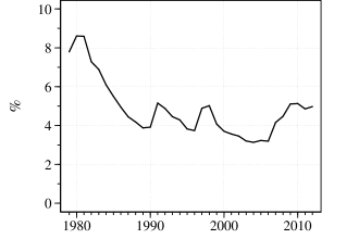
The proportion and characteristics of minimum wage workers serve as starting points for a discussion on the distributional impact of the minimum wage. According to the Current Population Survey (CPS), the proportion of workers who earn at or below the minimum wage in the United States ranges between 3 and 9 percent for the years 1979 to 2012 (Figure 1a). Less than 10 percent of workers have been directly affected by the minimum wage in the U.S. labor market. The extent to which the minimum wage affects the wage structure depends on the magnitude of the spillover effects on workers who earn more than the minimum wage. The minimum wage can exert a substantial influence on the wage structure if there are strong spillover effects.

Perhaps a less well-known fact is that minimum wage workers are concentrated in particular demographic groups. Approximately 90 percent of workers who earned at or below the minimum wage in the United States between the years 1979 and 2012 were high school graduates or less, younger than 25 years old, or female (Figure 1b). The reason was not that the minimum wage policy had been targeted based on education, experience, or gender, but because the lowest paid workers were mostly either less educated, young, or female. In light of this, the minimum wage may affect the relationship of hourly wages with education, experience, and gender.

Figure 1: Proportion and characteristics of minimum wage workers

(a) How many workers earn the minimum wage?

(b) Who earns the minimum wage?

Notes: Figure 1a is reproduced from Figure 2 in Autor et al. (2016). In Figure 1b, less-educated workers are those with a high school degree or less, and young workers are those aged 24 years or less.

Motivated by the fact above, we examine the distributional impact of the minimum wage in different ways from previous studies. We first consider a standard wage equation, in which the logarithm of real hourly wages is determined by education, experience and gender. We then look at changes in the distribution of wages resulting from the minimum wage through the lens of the wage equation. We allow the impact of the minimum wage to be heterogeneous with respect to unobserved, as well as observed, characteristics of workers, and for this purpose we adopt a quantile regression approach. Using quantile regression estimates, we evaluate the contribution of the minimum wage to changes in between- and within-group inequality.

We show that changes in the real value of the minimum wage over recent decades have affected the relationship of hourly wages with education, experience, and gender in the United States. The impact of the minimum wage is heterogeneous across workers depending on their observed characteristics. Consequently, changes in the real value of the minimum wage account in part for the patterns of changes in education, experience, and gender wage differentials. We further show that changes in the real value of the minimum wage over recent decades have affected wage differentials among workers with the same observed characteristics. The impact of the minimum wage is heterogeneous across quantiles of workers’ productivity not attributable to their observed characteristics. Consequently, changes in the real value of the minimum wage account mostly for the patterns of changes in within-group wage differential among workers with lower levels of experience.

The remainder of the paper is organized as follows. The next section reviews the related literature. Section 3 describes the data and institutional background. Section 4 presents an econometric framework to evaluate the quantitative contribution of the minimum wage to changes in between- and within-group inequality. Section 5 provides the empirical results. The final section concludes.

2 Related Literature

The literature has proven that the minimum wage has an effect on the distribution of hourly wages in the United States, while the magnitude and mechanisms of the effect vary across studies (DiNardo et al., 1996; Lee, 1999; Teulings, 2003; Autor et al., 2016). These studies develop and adopt different approaches that take into account different degrees of heterogeneity and spillovers in the impact of the minimum wage. DiNardo et al. (1996) develop a semiparametric approach to estimating discontinuous changes in the wage distribution at the minimum wage. Lee (1999) develop a semiparametric approach to estimating heterogeneous effects of the minimum wage across quantiles of the wage distribution. Teulings (2003) develops a parametric approach to estimating the impact of the minimum wage on the wage distribution. When comparing semiparametric approaches developed by DiNardo et al. (1996) and Lee (1999), DiNardo et al.’s (1996) approach allows for heterogeneous effects with respect to workers’ observed characteristics, while Lee’s (1999) approach does not. DiNardo et al.’s (1996) approach, however, requires additional assumptions to estimate the impact of the minimum wage from the cross-sectional distribution of wages. Consequently, DiNardo et al.’s (1996) approach does not allow for spillover effects, while Lee’s (1999) approach does. The approaches also differ in robustness to unobserved state and time effects. If there is sufficient variation in the minimum wage across states over time, Lee’s (1999) approach can separately identify the impact of the minimum wage from unobserved state and time effects. Autor et al. (2016) refine and apply Lee’s (1999) approach to data covering a longer period, and develop a test for the presence of spillover effects under a distributional assumption. However, no study has incorporated heterogeneous effects across workers with different observed characteristics in Lee’s (1999) approach.

Understanding the sources of changes in between- and within-group inequality is key to understanding the mechanisms of changes in wage inequality in the United States (Lemieux, 2006; Autor, Katz, and Kearney, 2008). However, little is known concerning the extent to which changes in between- and within-group wage differentials are attributed to changes in the real value of the minimum wage. In the literature, changes in between-group wage differentials have been typically attributed to changes in technology, workforce composition, and gender discrimination (see Katz and Autor, 1999; Blau and Kahn, 2017, for surveys). There is no consensus on the quantitative contribution of the minimum wage to changes in between-group wage differentials. DiNardo et al. (1996) and Lee (1999) conclude that changes in the educational wage differential are attributable only to a small extent to changes in the real value of the minimum wage, while Teulings (2003) concludes that changes in the educational wage differential are attributable to a large extent to changes in the real value of the minimum wage. DiNardo et al. (1996) demonstrate that the minimum wage was an important factor in accounting for changes in wage inequality in the 1980s. However, the literature identifying the sources of changes in within-group wage differentials have been less conclusive than the literature identifying the sources of changes in between-group wage differentials (Lemieux, 2006; Autor et al., 2008).

3 Data

The data used in our analysis are repeated cross-sectional data from the Current Population Survey Merged Outgoing Rotation Group. We construct variables in the same way as in Autor et al. (2016), and focus on the period between 1979 and 2012 to ensure the comparability of results. We restrict the sample to workers aged between 18 and 64 including males and females, full-time and part-time workers, but excluding self-employed workers, in the same way as in Autor et al. (2016). We, however, add in the sample individuals for whom we cannot observe wages. The yearly sample size ranges from 142,000 to 235,000. Following DiNardo et al. (1996), Lee (1999), and Autor et al. (2016), we weight each individual according to the sampling weight multiplied by hours worked.

Figure 2: The statutory minimum wage, 1979–2012

(a) Low minimum wage states (17 states)

(b) Medium minimum wage states (17 states)

(c) High minimum wage states (16 states)

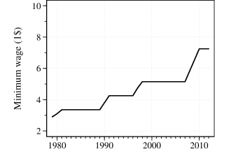
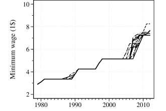
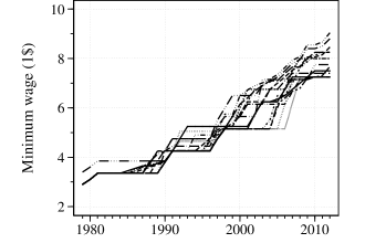
Notes: Panel (a) includes Alabama, Georgia, Idaho, Indiana, Kansas, Louisiana, Mississippi, North Dakota, Nebraska, Oklahoma, South Carolina, South Dakota, Tennessee, Texas, Utah, Virginia, and Wyoming. Panel (b) includes Arkansas, Arizona, Colorado, Kentucky, Maryland, Michigan, Minnesota, Missouri, Montana, North Carolina, New Hampshire, New Mexico, Nevada, Ohio, Pennsylvania, Wisconsin, and West Virginia. Panel (c) includes Alaska, California, Connecticut, Delaware, Florida, Hawaii, Iowa, Illinois, Massachusetts, Maine, New Jersey, New York, Oregon, Rhode Island, Vermont, and Washington.

Minimum wage laws differ across states and change over time in the United States. The federal government sets the federal minimum wage that applies to all states. State governments can set the state minimum wage higher than the federal minimum wage. The statutory minimum wage is the maximum of the federal minimum wage and the state minimum wage.

Figure 2 shows the trend in the statutory minimum wage. For ease of reference, we divide all 50 states evenly into three groups according to the level of statutory minimum wage. During the period, 17 states had no state minimum wage (Figure 2a). The statutory minimum wage equals the federal minimum wage in these states. The federal minimum wage increased four times: 1979 to 1981, 1989 to 1991, 1996 to 1998, and 2007 to 2010. The remaining 33 states set their state minimum wages (Figures 2b and 2c). The statutory minimum wage has been higher than the federal minimum wage for many years in these states. In the 1980s there was not much variation across states or changes over time in the minimum wage. On the other hand, in the 1990s and the 2000s there was substantial variation in the minimum wage across states over time.

Figure 3: The real value of the minimum wage, 1979–2012

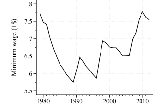
Notes: National averages are reported.

Figure 3 shows the national average trend in the real value of the minimum wage. The statutory minimum wage is deflated by the personal consumer expenditure price index using 2012 as the base year. During the period, there was a change in the trend in the year 1989. The real value of the minimum wage fell due to inflation from 1979 to 1989. Subsequently, the real value of the minimum wage exhibits an upward trend due to increases in the statutory minimum wage for the years 1989 to 2012.

4 Econometric Framework

In this section, we present our econometric framework. We start by introducing the (state-level) panel quantile regression model. Then, we describe the censored quantile regression model. We end this section by describing our approach to evaluating the quantitative contribution of the minimum wage to changes in between- and within-group inequality.

4.1 Model

The key feature of our model is that it allows the impact of the minimum wage to be heterogeneous with respect to workers’ observed and unobserved characteristics. This feature is essential for evaluating the contribution of the minimum wage to changes in between- and within-group inequality.

For the purpose of our analysis, we adopt the quantile regression approach pioneered by Koenker and Bassett (1978) and developed by Chetverikov, Larsen, and Palmer (2016). We have a repeated cross section of individuals $i=1,\ldots,N_{st}$ in states $s=1,\ldots,S$, and time $t=1,\ldots,T$. For each state and year, the structure of wages can be expressed using the following quantile regression model:

$$Q_{st}\left(\left.\tau\right|z_{ist}\right)=z_{ist}^{\prime}\alpha_{st}\left(\tau\right)\qquad\text{for \enskip}\tau\in\left(0,1\right),$$ (1)

where $Q_{st}\left(\left.\tau\right|z_{ist}\right)$ is the $\tau$th conditional quantile of the log of real hourly wages, $w_{ist}$, given a $J+1$ vector of observed individual characteristics, $z_{ist}$, for each state $s$ and year $t$. The vector of parameters $\alpha_{st}\left(\tau\right)$ can vary across quantiles $\tau$. The vector $z_{ist}$ includes a constant term, the linear and quadratic terms in years of education and of potential experience (age minus education minus six), and an indicator for being male. There are three reasons we use these variables. First, they are determined prior to the entry of the labor market. Second, they are commonly used as regressors in the quantile regression of wages (Buchinsky, 1994; Angrist, Chernozhukov, and Fernández-Val, 2006). Finally, and most importantly, they are useful to distinguish minimum wage workers. The quantile regression model (1) is more flexible than usual in that it allows all intercept and slope coefficients to vary across states and years.

Given the structure of wages described above, we examine the distributional impact of the minimum wage by looking at changes in the vector of coefficients, $\alpha_{st}\left(\tau\right)\equiv\bigl{(}\alpha_{0st}\left(\tau\right),\alpha_{1st}\left(\tau\right),\ldots,\alpha_{Jst}\left(\tau\right)\bigr{)}^{\prime}$, in equation (1) resulting from changes in the real value of the minimum wage. We consider the following (state-level) panel data model:

$$\alpha_{jst}\left(\tau\right)=m_{st}\beta_{j}\left(\tau\right)+x_{st}^{\prime}\gamma_{j}\left(\tau\right)+\epsilon_{jst}\left(\tau\right)\qquad\text{for }j=0,\ldots,J,$$ (2)

where $m_{st}$ is the log of the real value of the minimum wage, and $x_{st}$ is a vector of state-year characteristics. The vector $x_{st}$ includes state and year dummies and state-specific linear trends in the same way as in Autor et al. (2016). A set of parameters, $\beta\left(\tau\right)=\bigl{(}\beta_{0}\left(\tau\right),\beta_{1}\left(\tau\right),\ldots,\beta_{J}\left(\tau\right)\bigr{)}^{\prime}$, represents the heterogeneous impact of the minimum wage. Note that the first element of the vector $\boldsymbol{z}_{ist}$ is one. The second to last elements, $\beta_{1}\left(\tau\right)$ to $\beta_{J}\left(\tau\right)$, of the vector $\beta\left(\tau\right)$ measure the extent to which the impact of the minimum wage varies across individuals according to their observed characteristics. If the impact of the minimum wage is not heterogeneous with respect to observed characteristics, the parameter vector is $\beta\left(\tau\right)=\left(\beta_{0}\left(\tau\right),0,\ldots,0\right)^{\prime}$ for a given $\tau$. The quantile $\tau$ can be interpreted as the position in the distribution of workers’ productivity not attributable to their observed characteristics. If the impact of the minimum wage is not heterogeneous with respect to unobserved quantiles, the parameter vector is $\beta\left(\tau\right)=\left(\beta_{0},\beta_{1},\ldots,\beta_{J}\right)^{\prime}$ for all $\tau$.

Following Chetverikov et al. (2016), equations (1) and (2) can be estimated in two steps. In the first step, we perform separate quantile regressions of $w_{ist}$ by state $s$ and year $t$ for each quantile $\tau$ using the individual-level cross-sectional data. We then obtain a set of estimated parameters $\widehat{\alpha}_{st}\left(\tau\right)=\left(\widehat{\alpha}_{0,st}\left(\tau\right),\widehat{\alpha}_{1,st}\left(\tau\right),\ldots,\widehat{\alpha}_{J,st}\left(\tau\right)\right)^{\prime}$. In the second step, we perform the linear regression of $\widehat{\alpha}_{jst}\left(\tau\right)$ for each element $j$ and quantile $\tau$ using the state-level panel data. Relative to several applications discussed in Chetverikov et al. (2016), we allow for interactions between the treatment variable and individual characteristics, while we assume the exogeneity of the treatment variable. The minimum wage is commonly assumed to be exogenous in the literature. We, however, examine the possibility that differences in changes in the real value of the minimum wage across states may be driven by differences in changes in unobserved state characteristics.

The approach described above is related to the approach used in Lee (1999), who estimates the model of the form:

$$Q_{st}\left(\tau\right)-Q_{st}\left(0.5\right)=\bigl{(}m_{st}-Q_{st}\left(0.5\right)\bigr{)}\beta\left(\tau\right)+x_{st}^{\prime}\gamma\left(\tau\right)+\epsilon_{st}\left(\tau\right),$$ (3)

where $Q_{st}\left(\tau\right)$ is the $\tau$th unconditional quantile of $w_{ist}$. If the median wage, $Q_{st}\left(0.5\right)$, is absent, this model corresponds to the case in which all individual characteristics are excluded from equation (1). The main reason for the use of the median wage is presumably that there was insufficient variation in the state minimum wage during the period of the author’s analysis, 1979 to 1988.

4.2 Estimation

We address the issues of censoring and truncation, building on the approach described above.

Censoring

The wage distribution has been left-censored due to the minimum wage in many states (DiNardo et al., 1996; Lee, 1999). This issue is evident from the data but typically ignored when estimating the wage equation. The main reason, presumably, is that the magnitude of the bias due to left-censoring at the minimum wage is negligible if the interest lies at the mean impact. However, the magnitude of the bias may not be negligible if the interest lies at the distributional impact. The left-censoring due to the minimum wage can cause the fitted wage equation to be flat. In this case, the intercept coefficient becomes larger, while the slope coefficients become smaller. This effect is stronger at quantiles closer to the minimum wage. As a likely consequence, the censoring effect (the impact of the minimum wage at the minimum wage) may suffer from a downward bias, while the spillover effect (the impact of the minimum wage above the minimum wage) may suffer from an upward bias.

In addition, the earnings data from the CPS is right-censored due to top-coding. This issue has been widely recognized in the literature. Many studies using the CPS data make some adjustments for top-coding. Hubbard (2011) develops a maximum likelihood approach to addressing this issue under a distributional assumption, and shows that an increase in top-coded observations causes a serious bias in the trend in the gender wage differential. The trends in the education and experience wage differentials are also subject to the influence of top-coding.

We adopt the censored quantile regression approach developed in Powell (1986), Chernozhukov and Hong (2002), and Chernozhukov, Fernández-Val, and Kowalski (2015) to address the issue of censoring. This approach is semiparametric in the sense that it does not require a distributional assumption. We consider the following censored quantile regression model to deal with left-censoring due to the minimum wage and right-censoring due to top-coding.

$$Q_{st}\left(\left.\tau\right|\boldsymbol{z}_{ist}\right)=\begin{cases}m_{st}&\text{if }w_{ist}\leq m_{st},\\ z_{ist}^{\prime}\alpha_{st}\left(\tau\right)&\text{if }m_{st}<w_{ist}<c_{it}\\ c_{it}&\text{if }w_{ist}\geq c_{it},\end{cases},$$ (4)

where $c_{it}$ denotes the top-coded value. The key concept of this approach is to estimate the quantile regression model using the subsample of individuals who are unlikely to be left- or right-censored. Appendix A.2 details the estimation procedure.

Missing wages

There are diverse views on the employment effect of the minimum wage (Card and Krueger, 1995; Neumark and Wascher, 2008). Given the importance of this issue, a valid question may be whether changes in the wage distribution are due in part to a potential loss of employment resulting from a rise in the minimum wage. For the sake of discussion, we suppose that workers lose their jobs in the order of those with the lowest to highest productivity. In this case, percentile wages can mechanically increase even without any actual increase in wages. This implies that if the sample is restricted to employed individuals, the censoring effect and the spillover effect might be subject to an upward bias. The magnitude of the bias depends on the magnitude of the employment effect. We control for potential bias by imputing the wages of non-employed individuals.

Our approach builds on the quantile imputation approach developed in Yoon (2010) and Wei (2017). For the purpose of imputation, we use the censored quantile regression model, instead of the standard quantile regression, to take into account left- and right-censoring. In the process of imputation, we assume that non-employed individuals are less productive than median employed individuals, as is common in the literature on the gender wage differential (Johnson, Kitamura, and Neal, 2000). We allow for selection on unobservables in that sense. Appendix A.2 details the imputation procedure. Appendix A.3.1 provides the results without imputation.

Procedure

The estimation procedure is divided into three stages. First, we estimate the censored quantile regression model (4) using the sample of employed individuals and impute the wages of individuals for whom we cannot observe wages. Second, we estimate the censored quantile regression model (4) using the sample of employed and non-employed individuals, and obtain the estimates for intercept and slope coefficients $\widehat{\alpha}_{jst}\left(\tau\right)$ in the wage equation for $j=0$, $1$, $\ldots$, $5$, $s=1$, $2$, $\ldots$, $50$, $t=1979$, $1980$, $\ldots$, $2012$, and $\tau=0.04$, $0.05$, $\ldots$, $0.97$. Both in the first and second stages, we perform the separate regressions by state and year for each quantile. Finally, we estimate the linear regression model (2) of $\widehat{\alpha}_{jst}\left(\tau\right)$ using the state-level panel data.

Inference

Chetverikov et al. (2016) derive the asymptotic properties of estimators for parameters in equation (2). The authors show that estimation errors from the individual-level quantile regression are asymptotically negligible, if the size of the sample used in the individual-level quantile regression is sufficiently large relative to the size of the sample used in the state-level linear regression. Because the sample size may not be sufficiently large in the least populous states, we choose to report bootstrapped confidence intervals. We construct bootstrapped intervals from 500,000 bootstrap estimates obtained by repeating the individual-level censored quantile regression 500 times and then repeating the state-level linear regression 1,000 times for each quantile regression estimate. We allow for arbitrary forms of heteroscedasticity and serial correlation.

Specification checks

As is common when estimating the impact of the minimum wage on the wage distribution (DiNardo et al., 1996; Lee, 1999; Teulings, 2003; Autor et al., 2016), we focus primarily on the contemporaneous effect of the minimum wage. We estimate the following model in which we add the lag and lead variables, $m_{s,t-1}$ and $m_{s,t+1}$, to assess the validity of the model specification.

$$\alpha_{jst}\left(\tau\right)=m_{s,t-1}\beta_{j,-1}\left(\tau\right)+m_{st}\beta_{j,0}\left(\tau\right)+m_{s,t+1}\beta_{j,+1}\left(\tau\right)+x_{st}^{\prime}\gamma_{j}\left(\tau\right)+\epsilon_{jst}\left(\tau\right)\quad\text{for }j=0,\ldots,J.$$ (5)

If model (2) is correctly specified, we expect two restrictions to be satisfied. First, the long-term effect, $\beta_{j,-1}\left(\tau\right)+\beta_{j,0}\left(\tau\right)$, in model (5), would be the same as the contemporaneous effect, $\beta_{j}\left(\tau\right)$, in model (2). This restriction will be valid if the policy effect is well captured by the contemporaneous effect. Second, there would be no leading effect in model (5); that is, $\beta_{j,+1}\left(\tau\right)=0$. This restriction will not hold if changes in the real value of the minimum wage are driven by changes in unobserved state characteristics. We, thus, examine whether the long-term effect differs from the contemporaneous effect, and whether the leading effect differs from zero.

4.3 Measures of inequality

The aim of this paper is to evaluate the quantitative contribution of the minimum wage to changes in between- and within-group inequality. Here, we provide the definition of the two types of inequality, and describe the way to measure the contribution of the minimum wage along the lines of the model described above.

Figure 4: Inequality measures

(a) Between-group inequality

(b) Within-group inequality

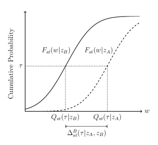
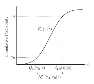
Notes: The conditional quantile function $Q_{st}\left(\left.\tau\right|z\right)$ is an inverse of $F_{st}\left(\left.w\right|z\right)$, where $F_{st}\left(\left.\cdot\right|z\right)$ is the conditional distribution function of $w_{ist}$ given $z_{ist}=z$ in state $s$ and year $t$.

Between-group inequality is the wage differential among workers with different observed characteristics. Consider two groups of workers, one of which consists of workers with individual characteristics, $z_{ist}=z_{A}$, and the other consists of workers with individual characteristics, $z_{ist}=z_{B}$. Between-group inequality can be defined as:

$$\Delta_{st}^{B}\left(\left.\tau\right|z_{A},z_{B}\right)\coloneqq Q_{st}\left(\left.\tau\right|z_{A}\right)-Q_{st}\left(\left.\tau\right|z_{B}\right)$$ (6)

for a given quantile $\tau$ (see Figure 4a for graphical description). Let $\widetilde{\Delta}_{st}^{B}$ denote the counterfactual between-group wage differential if the real value of the minimum wage were kept constant at a certain level. The contribution of the minimum wage can be measured by taking the difference between the actual wage differential and the counterfactual wage differential:

$$\Delta_{st}^{B}\left(\left.\tau\right|z_{A},z_{B}\right)-\widetilde{\Delta}_{st}^{B}\left(\left.\tau\right|z_{A},z_{B}\right).$$ (7)

Within-group inequality is the wage differential among workers with the same observed characteristics. Consider a range between two quantiles, $\tau_{A}$ and $\tau_{B}$, as a measure of inequality. Within-group inequality can be defined as:

$$\Delta_{st}^{W}\left(\left.\tau_{A},\tau_{B}\right|z\right)\coloneqq Q_{st}\left(\left.\tau_{A}\right|z\right)-Q_{st}\left(\left.\tau_{B}\right|z\right)$$ (8)

for a group of workers with individual characteristics, $z_{ist}=z$ (see Figure 4b for graphical description). Let $\widetilde{\Delta}_{st}^{W}$ denote the counterfactual within-group wage differential if the real value of the minimum wage is kept constant at a certain level. The contribution of the minimum wage can be measured by taking the difference between the actual wage differential and the counterfactual wage differential:

$$\Delta_{st}^{W}\left(\left.\tau_{A},\tau_{B}\right|z\right)-\widetilde{\Delta}_{st}^{W}\left(\left.\tau_{A},\tau_{B}\right|z\right).$$ (9)

5 Results

Our results are divided into two parts. The first part is a collection of the results regarding the impact of the minimum wage on the wage structure. The second part is a collection of the results regarding the contribution of the minimum wage to changes in between- and within-group inequality.

5.1 Impact on the wage structure

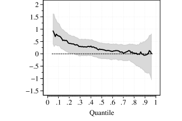
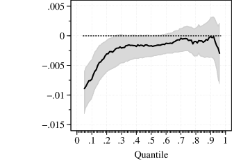
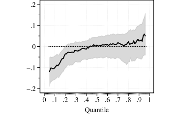
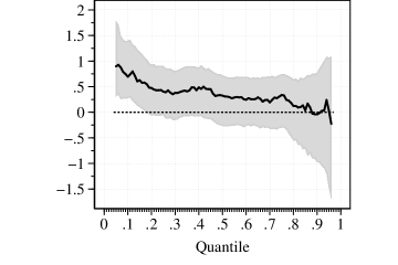
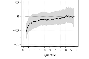
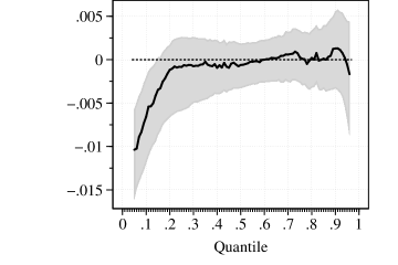
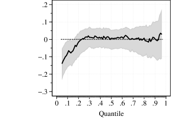
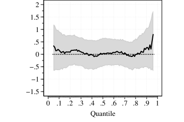
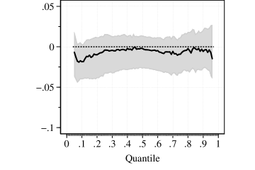
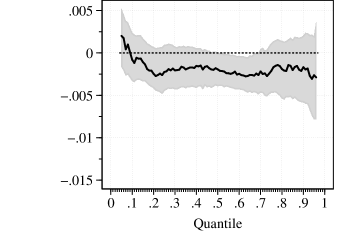
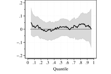
We first present the results of estimating equation (2). Figure 5 shows the impact of the minimum wage on the intercept and slope coefficients in the wage equation across quantiles. The four panels show the estimates for $\beta_{0}\left(\tau\right)$, $\beta_{1}\left(\tau\right)+2\beta_{2}\left(\tau\right)\overline{educ}$, $\beta_{3}\left(\tau\right)+2\beta_{4}\left(\tau\right)\overline{exper}$, and $\beta_{5}\left(\tau\right)$, respectively, where the bar represents the sample mean over all states and years. We summarize the impact of the minimum wage on the coefficients of linear and quadratic terms in education and experience as the impact on their marginal effects.

Figure 5: Impact of the minimum wage on the wage structure

(a) Intercept

(b) Education

(c) Experience

(d) Gender (male)

Notes: Estimates of partial effects in equation (2) are reported. The shaded area represents the 95 percent confidence interval. See Figure 17 for the uniform confidence band.

Both the intercept and slope coefficients in the wage equation are affected by the real value of the minimum wage. The intercept coefficient increases with a rise in the minimum wage (Figure 5a), while the slope coefficients of education, experience, and gender decrease with a rise in the minimum wage (Figures 5b, 5c, and 5d). The former result implies that a rise in the minimum wage results in a rise in the wages of the least-skilled workers in terms of observed characteristics. The latter result implies that a rise in the minimum wage weakens the relationship of hourly wages with education, experience, and gender. These results are consistent with the fact that less-educated, less-experienced, and female workers are more directly affected by a rise in the minimum wage than more-educated, more-experienced, and male workers. Furthermore, the magnitude of changes in the intercept and slope coefficients varies across quantiles. In all cases, the impact of the minimum wage is greatest at the lowest quantile and gradually declines in absolute value to zero by the 0.3 quantile. Spillover effects are present but limited mostly to the first quintile.

Figure 6: Long-term effect of the minimum wage on the wage structure

(a) Intercept

(b) Education

(c) Experience

(d) Gender (male)

Notes: Estimates of the long-term effects in equation (5) are reported. The shaded area represents the 95 percent confidence interval. See Figure 18 for the uniform confidence band.

Figure 7: Placebo effect on the wage structure

(a) Intercept

(b) Education

(c) Experience

(d) Gender (male)

Notes: Estimates of the leading effects in equation (5) are reported. The shaded area represents the 95 percent confidence interval. See Figure 19 for the uniform confidence band.

Lag and lead

Before discussing the contribution of the minimum wage to changes in between- and within-group inequality, we present the results when estimating the augmented equation (5). The four panels in Figure 6 show the estimates of the long-term effects. All estimates remain essentially unchanged, although they become less precise. Indeed, the long-term effects fall inside the 95 percent confidence intervals of the contemporary effects. The four panels in Figure 7 illustrate the estimates of the leading (placebo) effects. All estimates are close to zero for virtually all quantiles, and none of them are statistically significant. These results support our specification.

5.2 Contribution to changes in between- and within-group inequality

Finally, we discuss the quantitative contribution of the minimum wage to changes in between- and within-group inequality. As in Figure 3, the real value of the minimum wage declined by 30 log points due to inflation for the years 1979 to 1989 and subsequently increased by 28 log points due to increases in the statutory minimum wage for the years 1989 to 2012. Here, we provide the results for workers with 10 years of experience or less, who are subject to the influence of the minimum wage, for the latter period. Appendix A.3.2 shows the results for the former period.

5.2.1 Between-group inequality

Educational wage differential

We measure the educational wage differential by comparing workers with 16 years of education (equivalent to college graduates) and those with 12 years of education (equivalent to high school graduates), holding experience and gender constant. The four panels in Figure 8 show the national means of changes in the educational wage differential due to increases in the real value of the minimum wage for the years 1989 to 2012 by experience and gender for each decile $\tau=0.05$, $0.1$, $0.2$, …, $0.9$.

Figure 8: Changes in the educational wage differential (16 versus 12 years of education) due to the minimum wage, 1989–2012

(a) 5 years of experience, males

(b) 10 years of experience, males

(c) 5 years of experience, females

(d) 10 years of experience, females

Notes: Estimates of log-point changes in the educational wage differential due to the minimum wage are obtained from equation (7). The error bar represents the 95 percent confidence interval.

The minimum wage contributes to a reduction in the educational wage differential in the lower quantiles. The contribution of the minimum wage to a reduction in the educational wage differential is greater for more-experienced, female workers than less-experienced, male workers. For each group of workers, the contribution of the minimum wage is greatest at the 0.05th quantile and gradually declines in absolute value to zero by the 0.2th to 0.5th quantiles. For female workers with five years of experience, however, it is slightly greater at the 0.1th quantile than the 0.05th quantile. The reason is that, at the 0.05th quantile in this group, both more- and less-educated workers are affected by a rise in the real value of the minimum wage.

Figure 9: Actual and counterfactual changes in the educational wage differential (16 versus 12 years of education), 1989–2012

(a) 5 years of experience, males

(b) 10 years of experience, males

(c) 5 years of experience, females

(d) 10 years of experience, females

Notes: Actual and counterfactual log-point changes in the educational wage differential are obtained from equations (6) and (7).

The educational wage differential increased during the period (Figure 9). The trend in the educational wage differential is known to be important in accounting for the rise in wage inequality in the United States (Autor et al., 2008). The increase in the educational wage differential is typically attributed in the literature to skill-biased technological change and compositional changes in the workforce (Bound and Johnson, 1992; Katz and Murphy, 1992; Autor et al., 2008). The magnitude of the increase in the educational wage differential is greater in the higher quantiles than the lower quantiles during the period, as also shown by Buchinsky (1994) and Angrist et al. (2006). The educational wage differential did not increase at the 0.05 quantile and increased only moderately at the 0.1 quantile, while it increased more in the higher quantiles. If there were no increase in the real value of the minimum wage, however, the educational wage differential would increase at the 0.05 quantile and more than double at the 0.1 quantile for all groups. Consequently, in the counterfactual case in which the real value of the minimum wage is kept constant, the increase in the educational wage differential is more uniform across quantiles. Our results indicate that the minimum wage is another factor in accounting for the patterns of changes in the educational wage differential.

Experience wage differential

We measure the experience wage differential by comparing workers with 25 years of experience and those with five years of experience, holding education and gender constant. The four panels in Figure 10 show the national means of changes in the experience wage differential due to increases in the real value of the minimum wage for the years 1989 to 2012 by education and gender.

Figure 10: Changes in the experience wage differential (25 versus 5 years of experience) due to the minimum wage, 1989–2012

(a) 12 years of education, males

(b) 16 years of education, males

(c) 12 years of education, females

(d) 16 years of education, females

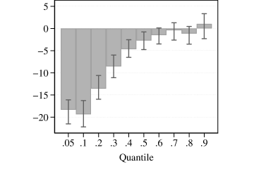
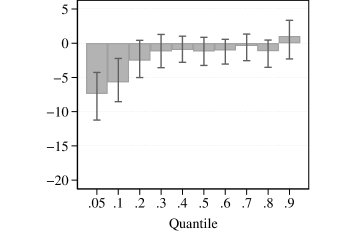
Notes: Estimates of log-point changes in the experience wage differential due to the minimum wage are obtained from equation (7). The error bar represents the 95 percent confidence interval.

The minimum wage contributes to a reduction in the experience wage differential in the lower quantiles. The contribution of the minimum wage to a reduction in the experience wage differential is greater for less-educated, female workers than more-educated, male workers. For each group of workers, the contribution of the minimum wage is greatest at the 0.05th quantile and gradually declines in absolute value to zero by the 0.2th to 0.5th quantiles. For female workers with 12 years of education, however, it is slightly greater at the 0.1th quantile than the 0.05th quantile. The reason is that, at the 0.05th quantile in this group, both more- and less-experienced workers are affected by a rise in the real value of the minimum wage.

Figure 11: Actual and counterfactual changes in the experience wage differential (25 versus 5 years of experience), 1989–2012

(a) 12 years of education, males

(b) 16 years of education, males

(c) 12 years of education, females

(d) 16 years of education, females

Notes: Actual and counterfactual log-point changes in the experience wage differential are obtained from equations (6) and (7).

The experience wage differential increased during the period with the exception of the lowest quantile (Figure 11). Changes in the experience wage differential are typically attributed in the literature to compositional changes in the workforce (Welch, 1979; Jeong, Kim, and Manovskii, 2015). The magnitude of the increase in the experience wage differential is greater in the higher quantiles than the lower quantiles during the period. The experience wage differential declined at the 0.05th quantile and increased only moderately at the median, while it increased more at the 0.7th and higher quantiles. If there were no increase in the real value of the minimum wage, however, the experience wage differential would increase in the lower as well as higher quantiles. Consequently, in the counterfactual case in which the real value of the minimum wage is kept constant, the increase in the educational wage differential at the 0.1th quantile is at least as high as the increase in the median for all groups. Our results indicate that the minimum wage is another factor in accounting for the patterns of changes in the experience wage differential.

Gender wage differential

We measure the gender wage differential by comparing male workers and female workers, holding education and experience constant. The four panels in Figure 12 show the national means of changes in the gender wage differential due to increases in the real value of the minimum wage for the years 1989 to 2012 by education and experience.

Figure 12: Changes in the gender wage differential (males versus females) due to the minimum wage, 1989–2012

(a) 12 years of education, 5 years of experience

(b) 12 years of education, 10 years of experience

(c) 16 years of education, 5 years of experience

(d) 16 years of education, 10 years of experience

Notes: Estimates of log-point changes in the gender wage differential due to the minimum wage are obtained from equation (7). The error bar represents the 95 percent confidence interval.

The minimum wage contributes to a reduction in the gender wage differential in the lower quantiles. The contribution of the minimum wage to a reduction in the gender wage differential is greater for less-educated, less-experienced workers than more-educated, more-experienced workers. For each group of workers, the contribution of the minimum wage is greatest at the 0.05th quantile and gradually declines in absolute value to zero by the 0.2th to 0.5th quantiles. For workers with 12 years of education and 5 years of experience, however, it is slightly greater at the 0.1th quantile than the 0.05th quantile. The reason is that, at the 0.05th quantile in this group, both male and female workers are affected by a rise in the real value of the minimum wage. For workers with 16 years of education, however, the contribution of the minimum wage is only modest across quantiles.

Figure 13: Actual and counterfactual changes in the gender wage differential (males versus females), 1989–2012

(a) 12 years of education, 5 years of experience

(b) 12 years of education, 10 years of experience

(c) 16 years of education, 5 years of experience

(d) 16 years of education, 10 years of experience

Notes: Actual and counterfactual log-point changes in the gender wage differential are obtained from equations (6) and (7).

The gender wage differential declined during the period (Figure 13). Changes in the gender wage differential are typically attributed in the literature to changes in workforce composition and gender discrimination (Blau and Kahn, 2017). Differently from the education and experience wage differentials, the magnitude of the change in the gender wage differential is almost uniform across quantiles. If there were no increase in the real value of the minimum wage, however, the gender wage differential would decline less in the lower quantiles. For workers with 12 years of education, the gender wage differential would not decline but could increase in the lower quantiles. Consequently, in the counterfactual case in which the real value of the minimum wage is kept constant, the decline in the gender wage differential is less in the lower quantiles than the higher quantiles for all groups. Our results indicate that the minimum wage is another factor in accounting for the patterns of changes in the gender wage differential.

5.2.2 Within-group inequality

The four panels in Figure 14 show the national means of changes in the 90/10 and 50/10 within-group wage differentials due to increases in the real value of the minimum wage for the years 1989 to 2012 by education, experience, and gender.

Figure 14: Changes in the 90/10, 50/10, and 50/20 within-group differentials due to the minimum wage, 1989–2012

(a) 90/10, males

(b) 90/10, females

(c) 50/10, males

(d) 50/10, females

(e) 50/20, males

(f) 50/20, females

Notes: Estimates of log-point changes in the within-group wage differentials due to the minimum wage are obtained from equation (9). The error bar represents the 95 percent confidence interval.

Figure 15: Actual and counterfactual changes in the 90/10, 50/10, and 50/20 within-group differentials, 1989–2012

(a) 90/10, males

(b) 90/10, females

(c) 50/10, males

(d) 50/10, females

(e) 50/20, males

(f) 50/20, females

Notes: Actual and counterfactual log-point changes in the within-group wage differentials are obtained from equations (8) and (9).

The minimum wage contributes to a reduction in the 90/10 and 50/10 within-group wage differentials among workers with lower levels of education and experience. The contribution of the minimum wage is the same for changes in the 90/10 and 50/10 within-group wage differentials except for female workers with 12 years of education and no experience. The results reflect the fact that changes in the real value of the minimum wage have no effect at the median or higher quantiles for almost all groups. The minimum wage also contributes to a reduction in the 50/20 within-group wage differential, but only moderately for fewer groups. The contribution of the minimum wage to changes in within-group wage differentials is greater for less-educated, less-experienced, female workers than more-educated, more-experienced, male workers. For workers with 16 years of education and five or more years of experience, the contribution of the minimum wage is close to zero.

The 90/10, 50/10, and 50/20 within-group wage differentials declined during the period (Figure 15). The 50/10 wage differential declined more than the 50/20 wage differential. The magnitude of the decline in within-group wage differentials is similar for male and female workers, but it is greater for less-educated, less-experienced workers than more-educated, more-experienced workers. If there were no increase in the minimum wage, however, the 50/10 and 50/20 wage differentials would change almost equally. Furthermore, within-group wage differentials would decline similarly for less-educated, less-experienced workers and more-educated, more-experienced workers, while they would decline less for male workers and would not decline but could increase for female workers. Our results indicate that the minimum wage accounts mostly for the patterns of changes in within-group wage differentials.

6 Conclusion

We have examined the impact of the minimum wage on the wage structure and evaluated the contribution of the minimum wage to changes in between- and within-group inequality in the United States. In doing so, we have addressed the issues of heterogeneity, censoring, and missing wages by combining three quantile regression approaches.

We have shown that changes in the real value of the minimum wage over recent decades have affected the relationship of hourly wages with education, experience, and gender. In the literature, changes in between-group wage differentials are typically attributed to skill-biased technological change, compositional changes in the workforce, and changes related to gender discrimination. Our results indicate that changes in the real value of the minimum wage account in part for the patterns of changes in the education, experience, and gender wage differentials. If there were no increase in the real value of the minimum wage in the 1990s and 2000s, the education and experience wage differentials would increase more uniformly across quantiles, while the gender wage differential would decline less uniformly across quantiles. Therefore, when we interpret the patterns of changes in between-group wage differentials through the lens of economic models, there is a need to adjust the data taking into account the influence of the minimum wage.

We have further shown that the impact of the minimum wage is heterogeneous across quantiles of workers’ productivity not attributable to their observed characteristics. In the literature, the sources of changes in within-group wage differentials are less conclusive than those of changes in between-group wage differentials. Our results indicate that changes in the real value of the minimum wage account mostly for the patterns of changes in within-group wage differentials for workers with 10 or less years of experience. In particular, the decline in the 50/10 and 50/20 within-group wage differential among female workers for the years 1989 to 2012 is attributed almost entirely to a rise in the real value of the minimum wage.

Appendix A Appendix

A.1 Conceptual framework

We provide a simple conceptual framework to understand the role of the minimum wage for the determination of the wage structure. Our model is related to and builds on the model in Bound and Johnson (1992) and Katz and Autor (1999). The key idea of the model is that the actual wage can be decomposed into the competitive market wage and the wedge. The wedge, which can be referred to as the rent, is a deviation of the actual wage from the competitive market wage.

The actual wage, $W_{ist}$, for an individual $i$ in state $s$ and year $t$ can be expressed as the product of the competitive market wage, $W_{t}^{c}$, in year $t$ and the rent, $R_{ist}$, for an individual $i$ in state $s$ and year $t$.

$$W_{ist}=W_{t}^{c}R_{ist}$$

The log of the actual wage, $w_{ist}$, can be decomposed additively into the log of the competitive market wage, $w_{t}^{c}$, and the log of the rent, $r_{ist}$.

$$w_{ist}=w_{t}^{c}+r_{ist}$$

In general, the rent is determined by state-specific institutional and non-competitive factors, $m_{st}$ and $\boldsymbol{x}_{st}$, and individual-specific productivity factors, $\boldsymbol{z}_{ist}$. Here, we consider the minimum wage to be a key institutional factor and allow for its interactive effect with individual characteristics.

$$R_{ist}=f\left(m_{st},x_{st},z_{ist}\right)=\exp\left[\left(z_{ist}^{\prime}\beta\right)m_{st}+\left(z_{ist}^{\prime}\otimes x_{st}^{\prime}\right)\gamma\right]$$

Given this functional form, the log wage equation can be derived as:

$$w_{ist}=z_{ist}^{\prime}\left[m_{st}\beta+\left(I_{J+1}\otimes x_{st}^{\prime}\right)\gamma\right],$$

where $I$ is an identity matrix, and $w_{t}^{c}$ is subsumed into $x_{st}$. The equation can be extended to allow for random coefficients.

$$w_{ist}=z_{ist}^{\prime}\left[m_{st}\beta\left(u\right)+\left(I_{J+1}\otimes x_{st}^{\prime}\right)\gamma\left(u\right)\right],$$

where $u$ represents unobserved individual characteristics, distributed uniformly from zero to one. This random coefficients model is an alternative representation of equations (1) and (2).

A.2 Estimation and imputation procedures

We describe the procedures for the censored quantile regression estimation and the quantile imputation. We implement the procedures for each state $s=1,\ldots,50$, each year $t=1979,1980,\ldots,2012$, and each quantile $\tau=0.04,0.05,\ldots,0.97$. In this section, we suppress the subscripts $s$ and $t$ for notational simplicity.

A.2.1 Censored quantile regression

The estimation proceeds in three steps (Chernozhukov and Hong, 2002). In the first and second steps, we select the sample to be used for estimation. In the third step, we estimate the quantile regression model using the selected sample.

Step 1.

We estimate the probabilities of not being left- and right-censored for each individual. When we partition the support of $\boldsymbol{z}_{i}$ into $\boldsymbol{\mathcal{Z}}_{1},\ldots,\mathcal{\boldsymbol{\mathcal{Z}}}_{H}$, we can nonparametrically estimate the probabilities of not being left- and right-censored from the empirical probabilities: $\widehat{p}^{L}\left(\boldsymbol{z}_{i}\right)\coloneqq\sum_{h=1}^{H}\widehat{p}_{h}^{L}\left\{\boldsymbol{z}_{i}\in\boldsymbol{\mathcal{Z}}_{h}\right\}$ and $\widehat{p}^{R}\left(\boldsymbol{z}_{i}\right)\coloneqq\sum_{h=1}^{H}\widehat{p}_{h}^{R}\left\{\boldsymbol{z}_{i}\in\boldsymbol{\mathcal{Z}}_{h}\right\}$, respectively, where for each $h$

$$\widehat{p}_{h}^{L}\left(\boldsymbol{z}_{i}\right)\coloneqq\frac{\sum_{i=1}^{N}\mathbbm{1}\left\{w_{i}>m,\boldsymbol{z}_{i}\in\boldsymbol{\mathcal{Z}}_{h}\right\}}{\sum_{i=1}^{N}\mathbbm{1}\left\{\boldsymbol{z}_{i}\in\boldsymbol{\mathcal{Z}}_{h}\right\}},\qquad\text{and}\qquad\widehat{p}_{h}^{R}\left(\boldsymbol{z}_{i}\right)\coloneqq\frac{\sum_{i=1}^{N}\mathbbm{1}\left\{w_{i}>c,\boldsymbol{z}_{i}\in\boldsymbol{\mathcal{Z}}_{h}\right\}}{\sum_{i=1}^{N}\mathbbm{1}\left\{\boldsymbol{z}_{i}\in\boldsymbol{\mathcal{Z}}_{h}\right\}}.$$

We partition the support of $\boldsymbol{z}_{i}$ by years of education (0–12, 12+), years of experience (0–9, 10–19, 20–29, 30+), and gender. Using the empirical probabilities, we select the sample:

$$\mathcal{I}_{1}\coloneqq\left\{i\in\left\{1,\ldots,N\right\}:1-\widehat{p}^{L}\left(\boldsymbol{z}_{i}\right)+\eta^{L}<\tau<\widehat{p}^{R}\left(\boldsymbol{z}_{i}\right)-\eta^{R}\right\},$$

where $\eta^{L}$ and $\eta^{R}$ are small positive constants to accommodate possible specification and estimation errors. Following Chernozhukov and Hong (2002), we set $\eta^{L}$ and $\eta^{R}$ at the 0.1th quantiles of the empirical probabilities of not being censored given $1-\widehat{p}^{L}\left(\boldsymbol{z}_{i}\right)<\tau$ and $\tau<\widehat{p}^{R}\left(\boldsymbol{z}_{i}\right)$, respectively.

Step 2.

We estimate the quantile regression model using the selected sample $\mathcal{I}_{1}$. Using a set of estimated coefficients $\widetilde{\boldsymbol{\alpha}}\left(\tau\right)$, we select the sample:

$$\mathcal{I}_{2}\coloneqq\left\{i\in\left\{1,\ldots,N\right\}:m+\zeta^{L}<\boldsymbol{z}_{i}^{\prime}\widetilde{\boldsymbol{\alpha}}\left(\tau\right)<c-\zeta^{R}\right\},$$

where $\zeta^{L}$ and $\zeta^{R}$ are small positive constants. Following Chernozhukov et al. (2015), we set $\eta^{L}$ and $\eta^{R}$ at the 0.03th quantiles of the positive fitted values of $\boldsymbol{z}_{i}^{\prime}\widetilde{\boldsymbol{\alpha}}\left(\tau\right)-m$ and $c_{i}-\boldsymbol{z}_{i}^{\prime}\widetilde{\boldsymbol{\alpha}}\left(\tau\right)$, respectively.

Step 3.

We estimate the quantile regression model using the selected sample $\mathcal{I}_{2}$.

A.2.2 Quantile imputation

The imputation proceeds in two steps (Wei, 2017).

Step 1.

We estimate the censored quantile regression model (4) using a sample of individuals for whom we can observe wages. We obtain a set of estimated coefficients $\left\{\widehat{\boldsymbol{\alpha}}\left(\tau\right):\tau\in\mathcal{T}^{\ast}\right\}$, where $\mathcal{T}^{\ast}\coloneqq\left\{0.04,0.05,\ldots,0.49\right\}$.

Step 2.

We draw a random variable, $u_{i}^{\ell}$, from a uniform distribution over $\mathcal{T}^{\ast}$ independently 10 times for individuals for whom we cannot their wages. For each realization of $u_{i}^{\ell}$, we predict their wages using the quantile regression model:

$$\widehat{w}_{i}^{\ell}\coloneqq\boldsymbol{z}_{i}^{\prime}\widehat{\boldsymbol{\alpha}}\bigl{(}u_{i}^{\ell}\bigr{)}.$$

If the predicted value is smaller than the minimum wage or greater than the top-coded value, it is replaced with the minimum wage or the top-coded value. We impute their wages by taking the mean of predicted values. We calculate their weights using hours worked imputed by fitting a fifth-order polynomial regression on wages.

A.3 Additional Results

Figure 16: Impact of the minimum wage on the wage structure without imputation

(a) Intercept

(b) Education

(c) Experience

(d) Gender (male)

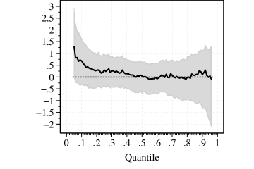
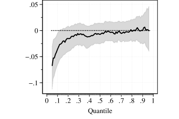
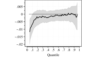
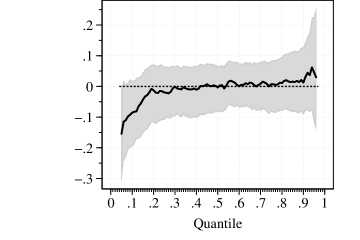
Notes: Estimates of partial effects in equation (2) are reported. The shaded area represents the 95 percent confidence interval.

A.3.1 Impact on the wage structure

Figure 16 shows the impact of the minimum wage on the intercept and slope coefficients in the wage equation across quantiles, when we do not impute the wages of individuals for whom we cannot observe wages. Both the intercept and slope coefficients in the wage equation are affected by the real value of the minimum wage in the same way as we see in Figure 5.

Figure 17: Impact of the minimum wage on the wage structure: confidence band

(a) Intercept

(b) Education

(c) Experience

(d) Gender (male)

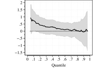
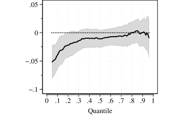
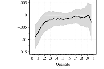
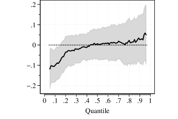
Notes: Estimates of partial effects in equation (2) are reported. The shaded area represents the 90 percent uniform confidence band.

Figures 17, 18, and 19 show uniform confidence bands of the estimates in Figures 5, 6, and 7, respectively. We follow Chernozhukov et al. (2013) in obtaining uniform confidence bands. Naturally, uniform confidence bands are wider than pointwise confidence intervals. However, we cannot reject the hypothesis of no effect of the minimum wage.

Figure 18: Long-term effect of the minimum wage on the wage structure: confidence band

(a) Intercept

(b) Education

(c) Experience

(d) Gender (male)

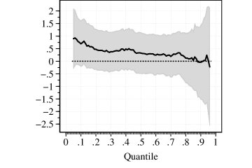
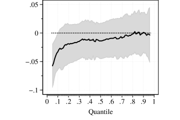
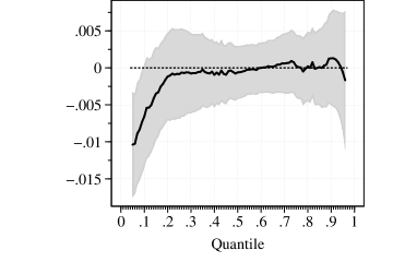
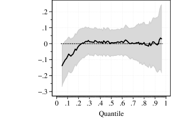
Notes: Estimates of the long-term effects in equation (5) are reported. The shaded area represents the 90 percent uniform confidence band.

Figure 19: Placebo effect on the wage structure: confidence band

(a) Intercept

(b) Education

(c) Experience

(d) Gender (male)

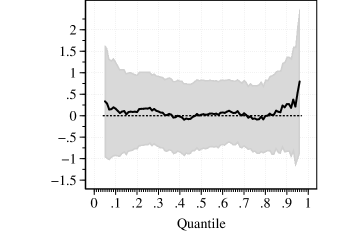
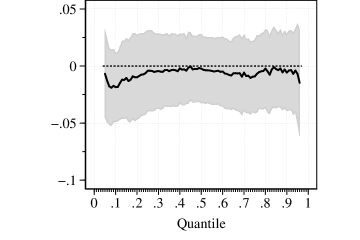
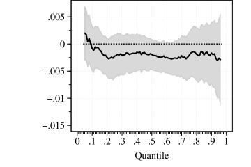
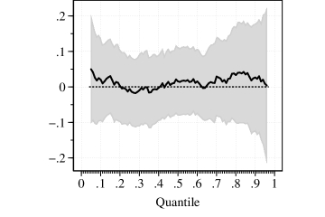
Notes: Estimates of the leading effects in equation (5) are reported. The shaded area represents the 90 percent uniform confidence band.

A.3.2 Changes in between- and within-group wage differentials, 1979–1989

Figures 20 to 23 show actual and counterfactual changes in between- and within-group wage differentials for the years 1979 to 1989.

Figure 20: Changes in the educational wage differential (16 versus 12 years of education), 1979–1989

(a) 5 years of experience, males

(b) 10 years of experience, males

(c) 5 years of experience, females

(d) 10 years of experience, females

During the 1979–1989 period, the educational wage differentials increased almost uniformly across quantiles (Figures 20), as also shown by Buchinsky (1994) and Angrist et al. (2006). If there were no decrease in the real value of the minimum wage, however, the educational wage differentials would increase less uniformly across quantiles.

The experience wage differentials also increased roughly uniformly, although they increased slightly more in the higher quantiles than the lower quantiles (Figures 21). If there were no decrease in the real value of the minimum wage, however, the experience wage differentials would increase more differently across quantiles.

Figure 21: Changes in the experience wage differential (25 versus 5 years of experience), 1979–1989

(a) 12 years of education, males

(b) 16 years of education, males

(c) 12 years of education, females

(d) 16 years of education, females

The gender wage differential declined more in the higher quantiles than the lower quantiles. If there were no decrease in the real value of the minimum wage, however, the gender wage differential would decline more uniformly across quantiles.

Figure 22: Changes in the gender wage differential (males versus females), 1979–1989

(a) 12 years of education, 5 years of experience

(b) 12 years of education, 10 years of experience

(c) 16 years of education, 5 years of experience

(d) 16 years of education, 10 years of experience

The 90/10, 50/10, and 50/20 within-group wage differentials changed little for male workers and increased for female workers. For female workers, the magnitude of the increase in within-group wage differentials is similar for less-educated and more-educated workers but greater for more-experienced than less-experienced workers. If there were no decrease in the real value of the minimum wage, however, within-group wage differentials would increase much less especially for workers with 5 or less years of experience.

Figure 23: Changes in the 90/10, 50/10, and 50/20 within-group differentials, 1979–1989

(a) 90/10, males

(b) 90/10, females

(c) 50/10, males

(d) 50/10, females

(e) 50/20, males

(f) 50/20, females

References

- Aaronson and French (2007) Aaronson, D. and E. French (2007): “Product Market Evidence on the Employment Effects of the Minimum Wage,” Journal of Labor Economics, 25, 167–200.
- Aaronson et al. (2018) Aaronson, D., E. French, I. Sorkin, and T. To (2018): “Industry Dynamics and the Minimum Wage: a Putty-clay Approach,” International Economic Review, 59, 51–84.
- Angrist et al. (2006) Angrist, J., V. Chernozhukov, and I. Fernández-Val (2006): “Quantile Regression under Misspecification, with an Application to the U.S. Wage Structure,” Econometrica, 74, 539–563.
- Autor et al. (2008) Autor, D. H., L. F. Katz, and M. S. Kearney (2008): “Trends in U.S. Wage Inequality: Revising the Revisionists,” Review of Economics and Statistics, 90, 300–323.
- Autor et al. (2016) Autor, D. H., A. Manning, and C. L. Smith (2016): “The Contribution of the Minimum Wage to US Wage Inequality over Three Decades: A Reassessment,” American Economic Journal: Applied Economics, 8, 58–99.
- Bell and Machin (2018) Bell, B. and S. Machin (2018): “Minimum Wages and Firm Value,” Journal of Labor Economics, 36, 159–195.
- Blau and Kahn (2017) Blau, F. D. and L. M. Kahn (2017): “The Gender Wage Gap: Extent, Trends, and Explanations,” Journal of Economic Literature, 55, 789–865.
- Bound and Johnson (1992) Bound, J. and G. Johnson (1992): “Changes in the Structure of Wages in the 1980’s: An Evaluation of Alternative Explanations,” American Economic Review, 82, 371–392.
- Buchinsky (1994) Buchinsky, M. (1994): “Changes in the U.S. Wage Structure 1963–1987: Application of Quantile Regression,” Econometrica, 62, 405–458.
- Card and Krueger (1995) Card, D. and A. B. Krueger (1995): Myth and Measurement, Princeton University Press.
- Card and Krueger (2017) ——— (2017): “Book Review: Myth and Measurement and the Theory and Practice of Labor Economics,” Industrial and Labor Relations Review, 70, 826–831.
- Chernozhukov et al. (2015) Chernozhukov, V., I. Fernández-Val, and A. E. Kowalski (2015): “Quantile Regression with Censoring and Endogeneity,” Journal of Econometrics, 186, 201–221.
- Chernozhukov et al. (2013) Chernozhukov, V., I. Fernández-Val, and B. Melly (2013): “Inference on Counterfactual Distributions,” Econometrica, 81, 2205–2268.
- Chernozhukov and Hong (2002) Chernozhukov, V. and H. Hong (2002): “Three-Step Censored Quantile Regression and Extramarital Affairs,” Journal of the American Statistical Association, 97, 872–888.
- Chetverikov et al. (2016) Chetverikov, D., B. Larsen, and C. Palmer (2016): “IV Quantile Regression for Group-Level Treatments, With an Application to the Distributional Effects of Trade,” Econometrica, 84, 809–833.
- DiNardo et al. (1996) DiNardo, J., N. M. Fortin, and T. Lemieux (1996): “Labor Market Institutions and the Distribution of Wages, 1973–1992: A Semiparametric Approach,” Econometrica, 64, 1001–1044.
- Draca et al. (2011) Draca, M., S. Machin, and J. V. Reenen (2011): “Minimum Wages and Firm Profitability,” American Economic Journal: Applied Economics, 3, 129–151.
- Dube (2018) Dube, A. (2018): “Minimum Wages and the Distribution of Family Incomes,” American Economic Journal: Applied Economics, forthcoming.
- Hubbard (2011) Hubbard, W. H. J. (2011): “The Phantom Gender Difference in the College Wage Premium,” Journal of Human Resources, 46, 568–586.
- Jeong et al. (2015) Jeong, H., Y. Kim, and I. Manovskii (2015): “The Price of Experience,” American Economic Review, 105, 784–815.
- Johnson et al. (2000) Johnson, W., Y. Kitamura, and D. Neal (2000): “Evaluating a Simple Method for Estimating Black-White Gaps in Median Wages,” American Economic Review Papers and Proceedings, 90, 339–343.
- Katz and Autor (1999) Katz, L. and D. Autor (1999): “Changes in the Wage Structure and Earnings Inequality,” Handbook of Labor Economics, 3A, 1463–1555.
- Katz and Murphy (1992) Katz, L. F. and K. M. Murphy (1992): “Changes in Relative Wages, 1963–1987: Supply and Demand Factors,” Quarterly Journal of Economics, 107, 35–78.
- Koenker (2017) Koenker, R. (2017): “Quantile Regression: 40 Years on,” Annual Review of Economics, 9, 155–176.
- Koenker and Bassett (1978) Koenker, R. and G. Bassett (1978): “Regression Quantiles,” Econometrica, 46, 33–50.
- Lee (1999) Lee, D. S. (1999): “Wage Inequality in the United States During the 1980s: Rising Dispersion or Falling Minimum Wage?” Quarterly Journal of Economics, 114, 977–1023.
- Lemieux (2006) Lemieux, T. (2006): “Increasing Residual Wage Inequality: Composition Effects, Noisy Data, or Rising Demand for Skill?” American Economic Review, 96, 461–498.
- Neumark and Wascher (2008) Neumark, D. and W. L. Wascher (2008): Minimum Wages, The MIT Press.
- Powell (1986) Powell, J. L. (1986): “Censored Regression Quantiles,” Journal of Econometrics, 32, 143–155.
- Teulings (2003) Teulings, C. N. (2003): “The Contribution of Minimum Wages to Increasing Wage Inequality,” The Economic Journal, 113, 801–803.
- Wei (2017) Wei, Y. (2017): “Quantile Regression with Measurement Errors and Missing Data,” in Handbook of Quantile Regression, ed. by R. Koenker, V. Chernozhukov, X. He, and L. Peng, Chapman and Hall/CRC.
- Welch (1979) Welch, F. (1979): “Effects of Cohort Size on Earnings: The Baby Boom Babies’ Financial Bust,” Journal of Political Economy, 87, S65–97.
- Yoon (2010) Yoon, J. (2010): “Quantile Regression Analysis with Missing Response with Applications to Inequality Measures and Data Combination,” Unpublished Manuscript.