Plane-strain waves in nonlinear elastic solids with softening

Harold Berjamin Bruno Lombard lombard@lma.cnrs-mrs.fr Aix-Marseille Univ, CNRS, Centrale Marseille, LMA, Marseille, France Guillaume Chiavassa Centrale Marseille, CNRS, Aix-Marseille Univ, M2P2 UMR 7340, 13451 Marseille Cedex 20, France Nicolas Favrie Aix-Marseille Univ, UMR CNRS 7343, IUSTI, Polytech Marseille, 13453 Marseille Cedex 13, France
Abstract

Propagation of elastic waves in damaged media (concrete, rocks) is studied theoretically and numerically. Such materials exhibit a nonlinear behavior, with long-time softening and recovery processes (slow dynamics). A constitutive model combining Murnaghan hyperelasticity with the slow dynamics is considered, where the softening is represented by the evolution of a scalar variable. The equations of motion in the Lagrangian framework are detailed. These equations are rewritten as a nonlinear hyperbolic system of balance laws, which is solved numerically using a finite-volume method with flux limiters. Numerical examples illustrate specific features of nonlinear elastic waves, as well as the effect of the material’s softening. In particular, the generation of solitary waves in a periodic layered medium is illustrated numerically.

keywords:
Nonlinear elastodynamics, softening, solitary waves, numerical methods
PACS:
43.25.Dc , 02.70.Bf
journal: Wave Motion

1 Introduction

Geomaterials such as rocks and concrete exhibit nonlinear features at small strains ε106similar-to𝜀superscript106\varepsilon\sim 10^{-6}. In particular, longitudinal resonance experiments reveal the generation of higher-order harmonics. Besides this phenomenon, the material exhibits also a softening with increasing strain amplitudes [1, 2]. After the forcing is stopped, the material recovers gradually its initial stiffness. This softening/recovery process is not instantaneous. The transient regime, named “slow dynamics” in the corresponding literature [3, 4, 5, 6], has a characteristic time much larger than the period of the forcing.

To describe nonlinear elastic behavior, the finite-strain theory is a self-consistent framework. Various constitutive laws of isotropic hyperelastic material express the stress as a function of a strain tensor, and are compatible with Hooke’s law in the infinitesimal strain limit [7, 8, 9]. Among them, the Murnaghan law [10] is frequently used to describe acoustic nonlinearity in rocks and concrete, and values of the parameters can be found in the literature [11, 12, 13]. However, hyperelasticity does not account for the long-time relaxation of elastic constants.

Several models from the literature describe the softening of the material by a dependence of the elastic constants on a scalar variable g𝑔g [14, 15, 16]. In the present study, the internal-variable model [16] is used, where the stress issued from Murnaghan’s law is multiplied by 1g1𝑔1-g. Hence, g0𝑔0g\equiv 0 corresponds to the hyperelastic case, and the material softens as g𝑔g increases. The evolution of g𝑔g is governed by a first-order differential equation compatible with the principles of thermodynamics. Both softening processes g˙0˙𝑔0\dot{g}\geqslant 0 and recovery processes g˙0˙𝑔0\dot{g}\leqslant 0 are possible [16], accordingly to the experimental observations.

In recent works [17], the corresponding one-dimensional equations of motion have been solved numerically using a finite-volume method with flux limiters [18]. The numerical method has been validated with respect to reference solutions, and qualitative agreement with experimental observations has been obtained. The present article describes a similar method in the two-dimensional plane-strain case. The numerical method is well-suited to the computation of nonlinear waves in the Lagrangian framework, and it can be used for various hyperelastic material models (cf. the related study [19] and references therein).

The article is organized as follows. In Section 2, the equations of motion are detailed, which are rewritten as a nonlinear hyperbolic system of balance laws in two space variables. The numerical method is presented in Section 3. Section 4 shows 2D numerical results illustrating the nonlinear wave propagation in elastic solids with softening. The case of a homogeneous medium is considered, as well as the case of a periodic layered medium with solitary wave solutions.

2 Governing equations

2.1 Lagrangian hyperelasticity with softening

We consider an homogeneous continuum. A particle initially located at some position 𝒙0subscript𝒙0\bm{x}_{0} of the reference configuration moves to a position 𝒙tsubscript𝒙𝑡\bm{x}_{t} of the deformed configuration. The deformation gradient is a second-order tensor defined by (see e.g. [7, 8, 20, 9])

𝑭=𝐠𝐫𝐚𝐝𝒙t=𝑰+𝐠𝐫𝐚𝐝𝒖,𝑭𝐠𝐫𝐚𝐝subscript𝒙𝑡𝑰𝐠𝐫𝐚𝐝𝒖\bm{F}=\mathbf{grad}\,\bm{x}_{t}=\bm{I}+\mathbf{grad}\,\bm{u}\,, (1)

where 𝒖=𝒙t𝒙0𝒖subscript𝒙𝑡subscript𝒙0\bm{u}=\bm{x}_{t}-\bm{x}_{0} denotes the displacement field and 𝐠𝐫𝐚𝐝𝐠𝐫𝐚𝐝\mathbf{grad} is the gradient with respect to the material coordinates 𝒙0subscript𝒙0\bm{x}_{0} (Lagrangian gradient). In the reference configuration, the deformation gradient (1) is equal to the metric tensor 𝑰𝑰\bm{I}. Here, the Euclidean space is described by an orthonormal basis (𝒆1,𝒆2,𝒆3)subscript𝒆1subscript𝒆2subscript𝒆3(\bm{e}_{1},\bm{e}_{2},\bm{e}_{3}) and a Cartesian coordinate system (O,x,y,z)𝑂𝑥𝑦𝑧(O,x,y,z), so that the matrix of the coordinates of 𝑰𝑰\bm{I} is the identity matrix.

The Lagrangian representation of motion is used. Hence, the material time derivative 𝑭˙=t𝑭˙𝑭subscript𝑡𝑭\dot{\bm{F}}=\partial_{t}\bm{F} of the deformation gradient satisfies

𝑭˙=𝐠𝐫𝐚𝐝𝒗,˙𝑭𝐠𝐫𝐚𝐝𝒗\dot{\bm{F}}=\mathbf{grad}\,\bm{v}\,, (2)

where 𝒗=𝒖˙𝒗˙𝒖\bm{v}=\dot{\bm{u}} is the velocity field. The conservation of mass implies ρ0/ρ=det𝑭subscript𝜌0𝜌𝑭{\rho_{0}}/{\rho}=\det\bm{F}, where ρ𝜌\rho denotes the mass density in the deformed configuration, and ρ0subscript𝜌0\rho_{0} denotes the mass density in the reference configuration. Self-gravitation and heat conduction are neglected, so that the motion is driven by the conservation of momentum

ρ0𝒗˙=𝐝𝐢𝐯𝑷+𝒇v,where𝑷=det(𝑭)𝝈𝑭formulae-sequencesubscript𝜌0˙𝒗𝐝𝐢𝐯𝑷superscript𝒇𝑣where𝑷𝑭𝝈superscript𝑭absenttop\rho_{0}\dot{\bm{v}}=\mathbf{div}\,\bm{P}+\bm{f}^{v}\,,\qquad\text{where}\qquad\bm{P}=\det(\bm{F})\,\bm{\sigma}\cdot\bm{F}^{-\top} (3)

is the first Piola–Kirchhoff stress tensor, and 𝐝𝐢𝐯𝐝𝐢𝐯\mathbf{div} denotes the divergence with respect to the material coordinates 𝒙0subscript𝒙0\bm{x}_{0}. The Cauchy stress tensor 𝝈=(det𝑭)1𝑷𝑭=𝝈𝝈superscript𝑭1𝑷superscript𝑭topsuperscript𝝈top\bm{\sigma}=(\det\bm{F})^{-1}\bm{P}\cdot\bm{F}^{\top}\!=\bm{\sigma}^{\top}\! is detailed later on through a specification of 𝑷𝑷\bm{P}. The term 𝒇vsuperscript𝒇𝑣\bm{f}^{v} is an external volume force applied to the material.

In hyperelasticity, the only variables of state are the specific entropy and a strain tensor. Here, the Green–Lagrange strain tensor 𝑬=12(𝑭𝑭𝑰)𝑬12superscript𝑭top𝑭𝑰\bm{E}=\frac{1}{2}(\bm{F}^{\top}\!\cdot\bm{F}-\bm{I}) is used, i.e.

𝑬=12(𝐠𝐫𝐚𝐝𝒖+𝐠𝐫𝐚𝐝𝒖+𝐠𝐫𝐚𝐝𝒖𝐠𝐫𝐚𝐝𝒖).𝑬12𝐠𝐫𝐚𝐝𝒖superscript𝐠𝐫𝐚𝐝top𝒖superscript𝐠𝐫𝐚𝐝top𝒖𝐠𝐫𝐚𝐝𝒖\bm{E}=\frac{1}{2}\left(\mathbf{grad}\,\bm{u}+\mathbf{grad}^{\top}\bm{u}+\mathbf{grad}^{\top}\bm{u}\cdot\mathbf{grad}\,\bm{u}\right). (4)

An internal variable g[0,1[g\in[0,1[ accounting for the softening of the material is added to the previous list of variables of state. We define the internal energy by unit of reference volume as [16]

ρ0e=(1g)W(𝑬)+Φ(g),subscript𝜌0𝑒1𝑔𝑊𝑬Φ𝑔\rho_{0}e=\left(1-g\right)W(\bm{E})+\Phi(g)\,, (5)

where e𝑒e is the specific internal energy. In (5), the potential W(𝑬)𝑊𝑬W(\bm{E}) is the strain energy function of Murnaghan’s law [10]

W(𝑬)=λ+2μ2EI22μEII+𝔩+2𝔪3EI32𝔪EIEII+𝔫EIII,𝑊𝑬𝜆2𝜇2superscriptsubscript𝐸I22𝜇subscript𝐸II𝔩2𝔪3superscriptsubscript𝐸I32𝔪subscript𝐸Isubscript𝐸II𝔫subscript𝐸IIIW(\bm{E})=\frac{\lambda+2\mu}{2}{E_{\text{I}}}^{2}-2\mu{E_{\text{II}}}+\frac{\mathfrak{l}+2\mathfrak{m}}{3}{E_{\text{I}}}^{3}-2\mathfrak{m}{E_{\text{I}}}{E_{\text{II}}}+\mathfrak{n}{E_{\text{III}}}\,, (6)

which is expressed as a function of the strain invariants EI=tr𝑬subscript𝐸Itr𝑬{E_{\text{I}}}=\text{tr}\,\bm{E}, EII=12((tr𝑬)2tr(𝑬2))subscript𝐸II12superscripttr𝑬2trsuperscript𝑬2{E_{\text{II}}}=\frac{1}{2}\big{(}(\text{tr}\,\bm{E})^{2}-\text{tr}(\bm{E}^{2})\big{)}, and EIII=det𝑬subscript𝐸III𝑬{E_{\text{III}}}=\det\bm{E}. The constants λ𝜆\lambda, μ𝜇\mu are the Lamé parameters and the constants 𝔩𝔩\mathfrak{l}, 𝔪𝔪\mathfrak{m}, 𝔫𝔫\mathfrak{n} are the Murnaghan coefficients (third-order elastic constants). In the case where the Murnaghan coefficients in (6) equal zero, the strain energy of the Saint Venant–Kirchhoff model is recovered. The potential Φ(g)Φ𝑔\Phi(g) represents a storage energy. Basic requirements are the convexity of ΦΦ\Phi and Φ(0)=0superscriptΦ00\Phi^{\prime}(0)=0, where ΦsuperscriptΦ\Phi^{\prime} is the derivative of ΦΦ\Phi (see [16]). Moreover, an asymptote at g=1𝑔1g=1 is introduced to avoid the destruction of the material. A suitable expression is

Φ(g)=12γln(1g2),Φ𝑔12𝛾1superscript𝑔2\Phi(g)=-\frac{1}{2}\gamma\ln(1-g^{2})\,, (7)

where γ>0𝛾0\gamma>0 is an energy per unit volume. The energy (7) is quadratic Φ(g)12γg2similar-to-or-equalsΦ𝑔12𝛾superscript𝑔2\Phi(g)\simeq\frac{1}{2}\gamma g^{2} in the limit g0𝑔0g\to 0.

Under the previous assumptions, the simplest set of constitutive equations with softening which is thermodynamically admissible reads [16]

𝑷=(1g)𝑭W𝑬,andτ1g˙=W(𝑬)Φ(g),formulae-sequence𝑷1𝑔𝑭𝑊𝑬andsubscript𝜏1˙𝑔𝑊𝑬superscriptΦ𝑔\bm{P}=\left(1-g\right)\bm{F}\cdot\frac{\partial W}{\partial\bm{E}}\,,\qquad\text{and}\qquad\tau_{1}\dot{g}=W(\bm{E})-\Phi^{\prime}(g)\,, (8)

where τ1>0subscript𝜏10\tau_{1}>0 in J m33-3 s is a material parameter. The first equation in (8) is the mechanical constitutive law, which reduces to the case of hyperelasticity if g0𝑔0g\equiv 0. According to the second equation in (8) which governs the evolution of the variable g𝑔g, the classical theory of nonlinear elastodynamics is recovered if τ1+subscript𝜏1\tau_{1}\to{+\infty}. Similarly to [16, 17], we rewrite the tensor derivative W/𝑬𝑊𝑬\partial W/\partial\bm{E} of the strain energy using the invariants’ tensor derivatives:

W𝑬=α0𝑰+α1𝑬+α2𝑬2,𝑊𝑬subscript𝛼0𝑰subscript𝛼1𝑬subscript𝛼2superscript𝑬2\frac{\partial W}{\partial\bm{E}}=\alpha_{0}\bm{I}+\alpha_{1}\bm{E}+\alpha_{2}\bm{E}^{2}, (9)

where

α0subscript𝛼0\displaystyle\alpha_{0} =WEI+EIWEII+EIIWEIIIabsent𝑊subscript𝐸Isubscript𝐸I𝑊subscript𝐸IIsubscript𝐸II𝑊subscript𝐸III\displaystyle=\frac{\partial W}{\partial{E_{\mathrm{I}}}}+E_{\mathrm{I}}\frac{\partial W}{\partial{E_{\mathrm{II}}}}+E_{\mathrm{II}}\frac{\partial W}{\partial{E_{\mathrm{III}}}}\! =λEI+𝔩EI2(2𝔪𝔫)EII,absent𝜆subscript𝐸I𝔩superscriptsubscript𝐸I22𝔪𝔫subscript𝐸II\displaystyle=\lambda E_{\mathrm{I}}+\mathfrak{l}{E_{\mathrm{I}}}^{2}-(2\mathfrak{m}-\mathfrak{n})E_{\mathrm{II}}\,, (10)
α1subscript𝛼1\displaystyle\alpha_{1} =WEIIEIWEIIIabsent𝑊subscript𝐸IIsubscript𝐸I𝑊subscript𝐸III\displaystyle=-\frac{\partial W}{\partial{E_{\mathrm{II}}}}-E_{\mathrm{I}}\frac{\partial W}{\partial{E_{\mathrm{III}}}}\! =2μ+(2𝔪𝔫)EI,absent2𝜇2𝔪𝔫subscript𝐸I\displaystyle=2\mu+(2\mathfrak{m}-\mathfrak{n})E_{\mathrm{I}}\,,
α2subscript𝛼2\displaystyle\alpha_{2} =WEIIIabsent𝑊subscript𝐸III\displaystyle=\frac{\partial W}{\partial{E_{\mathrm{III}}}}\! =𝔫.absent𝔫\displaystyle=\mathfrak{n}\,.

In the next subsection, we detail the case of plane strain. The case of uniaxial strain is addressed in [17].

2.2 The plane-strain assumption

The displacement field 𝒖𝒖\bm{u} is independent of z𝑧z, and its component u3subscript𝑢3u_{3} along 𝒆3subscript𝒆3\bm{e}_{3} is zero. In the basis of unit tensors (𝒆i𝒆j)1i,j3subscripttensor-productsubscript𝒆𝑖subscript𝒆𝑗formulae-sequence1𝑖𝑗3(\bm{e}_{i}\otimes\bm{e}_{j})_{1\leqslant i,j\leqslant 3}, the matrix of coordinates of the displacement gradient 𝐠𝐫𝐚𝐝𝒖𝐠𝐫𝐚𝐝𝒖\mathbf{grad}\,\bm{u} is therefore

(ui,j)=(u1,1u1,20u2,1u2,20000).matrixsubscript𝑢𝑖𝑗matrixsubscript𝑢11subscript𝑢120subscript𝑢21subscript𝑢220000\begin{pmatrix}u_{i,j}\end{pmatrix}={\begin{pmatrix}u_{1,1}&u_{1,2}&0\\ u_{2,1}&u_{2,2}&0\\ 0&0&0\end{pmatrix}}\,. (11)

Using the Einstein notation with indices in {1,2}12\{1,2\}, the coordinates of the Green–Lagrange tensor (4) write Eij=12(ui,j+uj,i+up,iup,j)subscript𝐸𝑖𝑗12subscript𝑢𝑖𝑗subscript𝑢𝑗𝑖subscript𝑢𝑝𝑖subscript𝑢𝑝𝑗E_{ij}=\frac{1}{2}\big{(}u_{i,j}+u_{j,i}+u_{p,i}u_{p,j}\big{)}. Its invariants in (6) are EI=Ennsubscript𝐸Isubscript𝐸𝑛𝑛E_{\text{I}}=E_{nn}, EII=12(EI2EijEij)=ϵijE1iE2jsubscript𝐸II12superscriptsubscript𝐸I2subscript𝐸𝑖𝑗subscript𝐸𝑖𝑗subscriptitalic-ϵ𝑖𝑗subscript𝐸1𝑖subscript𝐸2𝑗E_{\text{II}}=\frac{1}{2}\big{(}{E_{\text{I}}}^{2}-E_{ij}E_{ij}\big{)}=\epsilon_{ij}E_{1i}E_{2j} and EIII=0subscript𝐸III0E_{\text{III}}=0, where ϵijsubscriptitalic-ϵ𝑖𝑗\epsilon_{ij} is the Levi-Civita symbol of 2superscript2\mathbb{R}^{2}. The Cayley–Hamilton theorem applied to the restriction of 𝑬𝑬\bm{E} to 2×2superscript2superscript2\mathbb{R}^{2}\times\mathbb{R}^{2} reads EimEmjEIEij+EIIδij=0subscript𝐸𝑖𝑚subscript𝐸𝑚𝑗subscript𝐸Isubscript𝐸𝑖𝑗subscript𝐸IIsubscript𝛿𝑖𝑗0E_{im}E_{mj}-E_{\text{I}}E_{ij}+E_{\text{II}}\delta_{ij}=0, where δijsubscript𝛿𝑖𝑗\delta_{ij} is the Kronecker delta. Hence, the expression (9) of W/𝑬𝑊𝑬\partial W/\partial\bm{E} becomes

WEij=α~0δij+α~1Eij𝑊subscript𝐸𝑖𝑗subscript~𝛼0subscript𝛿𝑖𝑗subscript~𝛼1subscript𝐸𝑖𝑗\frac{\partial W}{\partial E_{ij}}=\tilde{\alpha}_{0}\delta_{ij}+\tilde{\alpha}_{1}E_{ij} (12)

in the basis of unit tensors (𝒆i𝒆j)1i,j2subscripttensor-productsubscript𝒆𝑖subscript𝒆𝑗formulae-sequence1𝑖𝑗2(\bm{e}_{i}\otimes\bm{e}_{j})_{1\leqslant i,j\leqslant 2}, where

α~0subscript~𝛼0\displaystyle\tilde{\alpha}_{0} =α0α2EIIabsentsubscript𝛼0subscript𝛼2subscript𝐸II\displaystyle=\alpha_{0}-\alpha_{2}E_{\mathrm{II}}\! =λEI+𝔩EI22𝔪EII,absent𝜆subscript𝐸I𝔩superscriptsubscript𝐸I22𝔪subscript𝐸II\displaystyle=\lambda E_{\text{I}}+\mathfrak{l}{E_{\text{I}}}^{2}-2\mathfrak{m}E_{\text{II}}\,, (13)
α~1subscript~𝛼1\displaystyle\tilde{\alpha}_{1} =α1+α2EIabsentsubscript𝛼1subscript𝛼2subscript𝐸I\displaystyle=\alpha_{1}+\alpha_{2}E_{\mathrm{I}}\! =2(μ+𝔪EI).absent2𝜇𝔪subscript𝐸I\displaystyle=2\left(\mu+\mathfrak{m}E_{\text{I}}\right).

The components Pijsubscript𝑃𝑖𝑗P_{ij} of the first Piola–Kirchhoff stress tensor 𝑷𝑷\bm{P} in (8) are therefore

Pij=(1g)(δim+ui,m)(α~0δmj+α~1Emj)subscript𝑃𝑖𝑗1𝑔subscript𝛿𝑖𝑚subscript𝑢𝑖𝑚subscript~𝛼0subscript𝛿𝑚𝑗subscript~𝛼1subscript𝐸𝑚𝑗P_{ij}=(1-g)\left(\delta_{im}+u_{i,m}\right)\left(\tilde{\alpha}_{0}\delta_{mj}+\tilde{\alpha}_{1}E_{mj}\right) (14)

under the plane strain assumption, which does not depend upon the third Murnaghan coefficient 𝔫𝔫\mathfrak{n}.

When the geometric nonlinearities are negligible, the Green–Lagrange strain tensor (4) is linearized with respect to 𝐠𝐫𝐚𝐝𝒖𝐠𝐫𝐚𝐝𝒖\mathbf{grad}\,\bm{u}, i.e. 𝑬12(𝐠𝐫𝐚𝐝𝒖+𝐠𝐫𝐚𝐝𝒖)=𝜺similar-to-or-equals𝑬12𝐠𝐫𝐚𝐝𝒖superscript𝐠𝐫𝐚𝐝top𝒖𝜺\bm{E}\simeq\frac{1}{2}\big{(}\mathbf{grad}\,\bm{u}+\mathbf{grad}^{\top}\bm{u}\big{)}=\bm{\varepsilon} reduces to the infinitesimal strain tensor. The coordinates Eijsubscript𝐸𝑖𝑗E_{ij} of 𝑬𝑬\bm{E} are replaced by the coordinates εij=12(ui,j+uj,i)subscript𝜀𝑖𝑗12subscript𝑢𝑖𝑗subscript𝑢𝑗𝑖\varepsilon_{ij}=\frac{1}{2}\big{(}u_{i,j}+u_{j,i}\big{)} of 𝜺𝜺\bm{\varepsilon}. Moreover, the first Piola–Kirchhoff stress tensor 𝑷𝑷\bm{P} is linearized with respect to 𝐠𝐫𝐚𝐝𝒖𝐠𝐫𝐚𝐝𝒖\mathbf{grad}\,\bm{u} too, i.e. 𝑭W/𝑬W/𝜺similar-to-or-equals𝑭𝑊𝑬𝑊𝜺\bm{F}\cdot\partial W/\partial\bm{E}\simeq\partial W/\partial\bm{\varepsilon}. Hence, the equation Pij=(1g)(α~0δij+α~1εij)subscript𝑃𝑖𝑗1𝑔subscript~𝛼0subscript𝛿𝑖𝑗subscript~𝛼1subscript𝜀𝑖𝑗P_{ij}=(1-g)\,\big{(}\tilde{\alpha}_{0}\delta_{ij}+\tilde{\alpha}_{1}\varepsilon_{ij}\big{)} replaces (14). Under this assumption, linear elastodynamics is recovered if g0𝑔0g\equiv 0 (i.e., τ1+subscript𝜏1\tau_{1}\to{+\infty} in (8)), and if the Murnaghan coefficients 𝔩𝔩\mathfrak{l}, 𝔪𝔪\mathfrak{m} in (13) are zero (see A for details).

2.3 System of balance laws

Under the plane-strain assumption, the equations of motion (2)-(3)-(8) are rewritten as a two-dimensional system of balance laws

t𝐪+x𝐟(𝐪)+y𝐠(𝐪)=𝐫(𝐪)+𝐬,subscript𝑡𝐪subscript𝑥𝐟𝐪subscript𝑦𝐠𝐪𝐫𝐪𝐬\partial_{t}\mathbf{q}+\partial_{x}\mathbf{f}(\mathbf{q})+\partial_{y}\mathbf{g}(\mathbf{q})=\mathbf{r}(\mathbf{q})+\mathbf{s}\,, (15)

where 𝐪=(u1,1,u1,2,u2,1,u2,2,v1,v2,g)𝐪superscriptsubscript𝑢11subscript𝑢12subscript𝑢21subscript𝑢22subscript𝑣1subscript𝑣2𝑔top\mathbf{q}=(u_{1,1},u_{1,2},u_{2,1},u_{2,2},v_{1},v_{2},g)^{\top}\! is the vector of unknowns. The expressions of the flux functions, the relaxation function and the source term are

𝐟(𝐪)=(v10v20P11/ρ0P21/ρ00),𝐠(𝐪)=(0v10v2P12/ρ0P22/ρ00),𝐫(𝐪)=1τ1(000000WΦ(g)),𝐬=1ρ0(0000𝒇v𝒆1𝒇v𝒆20).formulae-sequence𝐟𝐪matrixsubscript𝑣10subscript𝑣20subscript𝑃11subscript𝜌0subscript𝑃21subscript𝜌00formulae-sequence𝐠𝐪matrix0subscript𝑣10subscript𝑣2subscript𝑃12subscript𝜌0subscript𝑃22subscript𝜌00formulae-sequence𝐫𝐪1subscript𝜏1matrix000000𝑊superscriptΦ𝑔𝐬1subscript𝜌0matrix0000superscript𝒇𝑣subscript𝒆1superscript𝒇𝑣subscript𝒆20\mathbf{f}(\mathbf{q})=-{\begin{pmatrix}v_{1}\\ 0\\ v_{2}\\ 0\\ P_{11}/\rho_{0}\\ P_{21}/\rho_{0}\\ 0\end{pmatrix}}\,,\quad\mathbf{g}(\mathbf{q})=-{\begin{pmatrix}0\\ v_{1}\\ 0\\ v_{2}\\ P_{12}/\rho_{0}\\ P_{22}/\rho_{0}\\ 0\end{pmatrix}}\,,\quad\mathbf{r}(\mathbf{q})=\frac{1}{\tau_{1}}{\begin{pmatrix}0\\ 0\\ 0\\ 0\\ 0\\ 0\\ W-\Phi^{\prime}(g)\end{pmatrix}}\,,\quad\mathbf{s}=\frac{1}{\rho_{0}}{\begin{pmatrix}0\\ 0\\ 0\\ 0\\ \bm{f}^{v}\!\cdot\bm{e}_{1}\\ \bm{f}^{v}\!\cdot\bm{e}_{2}\\ 0\end{pmatrix}}\,. (16)

In (16), the Piola–Kirchhoff stress components (Pij)1i,j2subscriptsubscript𝑃𝑖𝑗formulae-sequence1𝑖𝑗2(P_{ij})_{1\leqslant i,j\leqslant 2} depend on (ui,j)1i,j2subscriptsubscript𝑢𝑖𝑗formulae-sequence1𝑖𝑗2(u_{i,j})_{1\leqslant i,j\leqslant 2} and g𝑔g according to (14). The strain energy W𝑊W depends on (ui,j)1i,j2subscriptsubscript𝑢𝑖𝑗formulae-sequence1𝑖𝑗2(u_{i,j})_{1\leqslant i,j\leqslant 2} according to (6).

The Jacobian matrix of the flux component 𝐟𝐟\mathbf{f} along the x𝑥x-axis is

𝐟(𝐪)=(100000010000Q1111Q1112Q1121Q112200G11Q2111Q2112Q2121Q212200G210000000),superscript𝐟𝐪matrixmissing-subexpressionmissing-subexpressionmissing-subexpressionmissing-subexpression100missing-subexpressionmissing-subexpressionmissing-subexpressionmissing-subexpression000missing-subexpressionmissing-subexpressionmissing-subexpressionmissing-subexpression010missing-subexpressionmissing-subexpressionmissing-subexpressionmissing-subexpression000subscript𝑄1111subscript𝑄1112subscript𝑄1121subscript𝑄112200subscript𝐺11subscript𝑄2111subscript𝑄2112subscript𝑄2121subscript𝑄212200subscript𝐺210000000\mathbf{f}^{\prime}(\mathbf{q})=-{\begin{pmatrix}&&&&1&0&0\\ &&&&0&0&0\\ &&&&0&1&0\\ &&&&0&0&0\\ Q_{1111}&Q_{1112}&Q_{1121}&Q_{1122}&0&0&G_{11}\\ Q_{2111}&Q_{2112}&Q_{2121}&Q_{2122}&0&0&G_{21}\\ 0&0&0&0&0&0&0\end{pmatrix}}\,, (17)

where only three strips are displayed (everywhere else, the coefficients in the matrix are zero). The expression of the coefficients Qijksubscript𝑄𝑖𝑗𝑘Q_{ijk\ell} in (17) defined by ρ0Qijk=Pij/uk,subscript𝜌0subscript𝑄𝑖𝑗𝑘subscript𝑃𝑖𝑗subscript𝑢𝑘\rho_{0}Q_{ijk\ell}=\partial P_{ij}/\partial u_{k,\ell} is detailed in the A, as well as the expression of the coefficients Gijsubscript𝐺𝑖𝑗G_{ij} defined by ρ0Gij=Pij/gsubscript𝜌0subscript𝐺𝑖𝑗subscript𝑃𝑖𝑗𝑔\rho_{0}G_{ij}=\partial P_{ij}/\partial g. A similar Jacobian matrix 𝐠(𝐪)superscript𝐠𝐪\mathbf{g}^{\prime}(\mathbf{q}) is obtained for the flux component 𝐠𝐠\mathbf{g} along the y𝑦y-axis. These matrices are diagonalized in the A. The spectrum of both matrices has the form {cP,cP,cS,cS,0,0,0}subscript𝑐𝑃subscript𝑐𝑃subscript𝑐𝑆subscript𝑐𝑆000\{-c_{P},c_{P},-c_{S},c_{S},0,0,0\}. In the case of Murnaghan hyperelasticity, the eigenvalues cPsubscript𝑐𝑃c_{P}, cSsubscript𝑐𝑆c_{S} can be complex [17], so that the system (15)-(16) is not unconditionally hyperbolic (see e.g. [21] for discussions on hyperbolicity in hyperelasticity). Here, we restrict ourselves to configurations where the eigenvalues cP>cS>0subscript𝑐𝑃subscript𝑐𝑆0c_{P}>c_{S}>0 are real. Thus, cPsubscript𝑐𝑃c_{P} and cSsubscript𝑐𝑆c_{S} correspond to the velocities of compression waves and shear waves, respectively.

Plane waves

We assume furthermore that the displacement field is invariant along a direction, say 𝒆2subscript𝒆2\bm{e}_{2}, so that 𝒖𝒖\bm{u} does not depend on y𝑦y. In this case, the vector of unknown reduces to 𝐪=(u1,1,u2,1,v1,v2,g)𝐪superscriptsubscript𝑢11subscript𝑢21subscript𝑣1subscript𝑣2𝑔top\mathbf{q}=(u_{1,1},u_{2,1},v_{1},v_{2},g)^{\top}\! — the second and fourth rows of (15)-(16) are zero — and the flux 𝐠𝐠\mathbf{g} along y𝑦y is zero. The Jacobian matrix 𝐟(𝐪)superscript𝐟𝐪\mathbf{f}^{\prime}(\mathbf{q}) is obtained from (17) by removing the second and fourth rows, as well as the second and fourth columns. Doing so, two zero eigenvalues are removed from the spectrum, which reduces to {cP,cP,cS,cS,0}subscript𝑐𝑃subscript𝑐𝑃subscript𝑐𝑆subscript𝑐𝑆0\{-c_{P},c_{P},-c_{S},c_{S},0\}.

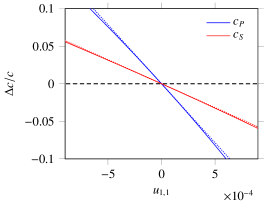
We consider the case of Murnaghan material g0𝑔0g\equiv 0, with the parameters in Table 1. The latter, found in [13], have been measured on concrete. Let us introduce the relative variation Δc/cΔ𝑐𝑐\Delta c/c of the sound velocities cPsubscript𝑐𝑃c_{P} and cSsubscript𝑐𝑆c_{S} with respect to the case of Hooke’s law, where cP=(λ+2μ)/ρ04458subscript𝑐𝑃𝜆2𝜇subscript𝜌04458c_{P}=\sqrt{(\lambda+2\mu)/\rho_{0}}\approx 4458 m/s and cS=μ/ρ02700subscript𝑐𝑆𝜇subscript𝜌02700c_{S}=\sqrt{\mu/\rho_{0}}\approx 2700 m/s. Fig. 1 displays the evolution of Δc/cΔ𝑐𝑐\Delta c/c with respect to the compression strain u1,1subscript𝑢11u_{1,1}, when the shear strain u2,1subscript𝑢21u_{2,1} is set to zero. One observes that the variations of cPsubscript𝑐𝑃c_{P} with respect to u1,1subscript𝑢11u_{1,1} are much larger than the variations of cSsubscript𝑐𝑆c_{S}. This is confirmed by the Taylor series approximations

(Δc/c)PsubscriptΔ𝑐𝑐𝑃\displaystyle(\Delta c/c)_{P} =(32+𝔩+2𝔪λ+2μ)u1,1+O(u1,12)+O(u2,12)157u1,1,absent32𝔩2𝔪𝜆2𝜇subscript𝑢11𝑂superscriptsubscript𝑢112𝑂superscriptsubscript𝑢212157subscript𝑢11\displaystyle=\left(\frac{3}{2}+\frac{\mathfrak{l}+2\mathfrak{m}}{\lambda+2\mu}\right)u_{1,1}+O({u_{1,1}}^{2})+O({u_{2,1}}^{2})\approx{-157}\,u_{1,1}\,, (18)
(Δc/c)SsubscriptΔ𝑐𝑐𝑆\displaystyle(\Delta c/c)_{S} =(λ+2μ2μ+𝔪2μ)u1,1+O(u1,12)+O(u2,12)63.8u1,1,absent𝜆2𝜇2𝜇𝔪2𝜇subscript𝑢11𝑂superscriptsubscript𝑢112𝑂superscriptsubscript𝑢21263.8subscript𝑢11\displaystyle=\left(\frac{\lambda+2\mu}{2\mu}+\frac{\mathfrak{m}}{2\mu}\right)u_{1,1}+O({u_{1,1}}^{2})+O({u_{2,1}}^{2})\approx{-63.8}\,u_{1,1}\,,

represented as dotted lines in Fig. 1 (the magnitude of u1,1subscript𝑢11u_{1,1} in the figure has been chosen for graphical reasons). These approximations show also that the shear strain u2,1subscript𝑢21u_{2,1} has much less influence than the compression strain u1,1subscript𝑢11u_{1,1} on the variations of the sound velocities.

Table 1: Physical parameters of concrete.
ρ0subscript𝜌0\rho_{0} (kg m33-3) λ𝜆\lambda (GPa) μ𝜇\mu (GPa) 𝔩𝔩\mathfrak{l} (GPa) 𝔪𝔪\mathfrak{m} (GPa) γ𝛾\gamma (J m 33-3) τ1subscript𝜏1\tau_{1} (J m33-3 s)
240024002400 12.712.712.7 17.517.517.5 30073007-3007 22832283-2283 4.0×1024.0superscript1024.0\times 10^{-2} 2.0×1062.0superscript1062.0\times 10^{-6}
Refer to caption
Figure 1: Murnaghan hyperelasticity (g0𝑔0g\equiv 0). Relative variation Δc/cΔ𝑐𝑐\Delta c/c of the speeds cPsubscript𝑐𝑃c_{P} and cSsubscript𝑐𝑆c_{S} of compressional and shear waves with respect to the case of Hooke’s law. The variation Δc/cΔ𝑐𝑐\Delta c/c is represented with respect to the compression strain u1,1subscript𝑢11u_{1,1}, and the shear strain is u2,1=0subscript𝑢210u_{2,1}=0. The dotted lines mark Taylor series approximations (18).

3 Numerical resolution

3.1 Numerical strategy

In the examples presented later on, the physical domain is assumed unbounded. We consider a finite numerical domain [0,Lx]×[0,Ly]0subscript𝐿𝑥0subscript𝐿𝑦[0,L_{x}]\times[0,L_{y}]. It is discretized using a regular grid in space with mesh size ΔxΔ𝑥\Delta x in the x𝑥x direction, and ΔyΔ𝑦\Delta y in the y𝑦y direction. The coordinates of the nodes are (xi,yj)=(iΔx,jΔy)subscript𝑥𝑖subscript𝑦𝑗𝑖Δ𝑥𝑗Δ𝑦(x_{i},y_{j})=(i\,\Delta x,j\,\Delta y), where 0iNx0𝑖subscript𝑁𝑥0\leqslant i\leqslant N_{x} and 0jNy0𝑗subscript𝑁𝑦0\leqslant j\leqslant N_{y}. The total number of nodes is (Nx+1)×(Ny+1)subscript𝑁𝑥1subscript𝑁𝑦1(N_{x}+1)\times(N_{y}+1), where Nx=Lx/Δxsubscript𝑁𝑥subscript𝐿𝑥Δ𝑥N_{x}=L_{x}/\Delta x and Ny=Ly/Δysubscript𝑁𝑦subscript𝐿𝑦Δ𝑦N_{y}=L_{y}/\Delta y. A variable time step Δt=tn+1tnΔ𝑡subscript𝑡𝑛1subscript𝑡𝑛\Delta t=t_{n+1}-t_{n} is introduced. Therefore, 𝐪(xi,yj,tn)𝐪subscript𝑥𝑖subscript𝑦𝑗subscript𝑡𝑛\mathbf{q}(x_{i},y_{j},t_{n}) denotes the solution to (15) at the grid node (i,j)𝑖𝑗(i,j) and at the n𝑛nth time step. Numerical approximations of the solution are denoted by 𝐪i,jn𝐪(xi,yj,tn)similar-to-or-equalssuperscriptsubscript𝐪𝑖𝑗𝑛𝐪subscript𝑥𝑖subscript𝑦𝑗subscript𝑡𝑛\mathbf{q}_{i,j}^{n}\simeq\mathbf{q}(x_{i},y_{j},t_{n}).

The non-homogeneous system of balance laws (15) is integrated explicitly in time:

𝐪i,jn+1=𝐪i,jn+Δ𝐪FVn+Δt(𝐫(𝐪i,jn)+𝐬i,jn),superscriptsubscript𝐪𝑖𝑗𝑛1superscriptsubscript𝐪𝑖𝑗𝑛Δsuperscriptsubscript𝐪FV𝑛Δ𝑡𝐫superscriptsubscript𝐪𝑖𝑗𝑛superscriptsubscript𝐬𝑖𝑗𝑛\mathbf{q}_{i,j}^{n+1}=\mathbf{q}_{i,j}^{n}+\Delta\mathbf{q}_{\text{FV}}^{n}+\Delta t\left(\mathbf{r}(\mathbf{q}_{i,j}^{n})+\mathbf{s}_{i,j}^{n}\right), (19)

where the approximation 𝐬i,jnsuperscriptsubscript𝐬𝑖𝑗𝑛\mathbf{s}_{i,j}^{n} of the source term 𝐬𝐬\mathbf{s} is specified later on. The increment Δ𝐪FVnΔsuperscriptsubscript𝐪FV𝑛\Delta\mathbf{q}_{\text{FV}}^{n} is deduced from the integration of t𝐪+x𝐟(𝐪)+y𝐠(𝐪)=𝟎subscript𝑡𝐪subscript𝑥𝐟𝐪subscript𝑦𝐠𝐪0\partial_{t}\mathbf{q}+\partial_{x}\mathbf{f}(\mathbf{q})+\partial_{y}\mathbf{g}(\mathbf{q})=\mathbf{0} over one time step. Usually, one has Δ𝐪FVn=(x+y2)𝐪i,jnΔsuperscriptsubscript𝐪FV𝑛subscript𝑥subscript𝑦2superscriptsubscript𝐪𝑖𝑗𝑛\Delta\mathbf{q}_{\text{FV}}^{n}=(\mathcal{H}_{x}+\mathcal{H}_{y}-2)\,\mathbf{q}_{i,j}^{n}, where the discrete operators

x𝐪i,jnsubscript𝑥superscriptsubscript𝐪𝑖𝑗𝑛\displaystyle\mathcal{H}_{x}\mathbf{q}_{i,j}^{n} =𝐪i,jnΔtΔx(𝐟i+1/2,jn𝐟i1/2,jn),absentsuperscriptsubscript𝐪𝑖𝑗𝑛Δ𝑡Δ𝑥superscriptsubscript𝐟𝑖12𝑗𝑛superscriptsubscript𝐟𝑖12𝑗𝑛\displaystyle=\mathbf{q}_{i,j}^{n}-\frac{\Delta t}{\Delta x}\left(\mathbf{f}_{i+1/2,j}^{n}-\mathbf{f}_{i-1/2,j}^{n}\right), (20)
y𝐪i,jnsubscript𝑦superscriptsubscript𝐪𝑖𝑗𝑛\displaystyle\mathcal{H}_{y}\mathbf{q}_{i,j}^{n} =𝐪i,jnΔtΔy(𝐠i,j+1/2n𝐠i,j1/2n),absentsuperscriptsubscript𝐪𝑖𝑗𝑛Δ𝑡Δ𝑦superscriptsubscript𝐠𝑖𝑗12𝑛superscriptsubscript𝐠𝑖𝑗12𝑛\displaystyle=\mathbf{q}_{i,j}^{n}-\frac{\Delta t}{\Delta y}\left(\mathbf{g}_{i,j+1/2}^{n}-\mathbf{g}_{i,j-1/2}^{n}\right),

involve the fluxes 𝐟i+1/2,jnsuperscriptsubscript𝐟𝑖12𝑗𝑛\mathbf{f}_{i+1/2,j}^{n}, 𝐠i+1/2,jnsuperscriptsubscript𝐠𝑖12𝑗𝑛\mathbf{g}_{i+1/2,j}^{n} of a 2D finite-volume scheme [18]. Here, a second-order symmetric dimensional splitting [22] is used instead. That is to say, xsubscript𝑥\mathcal{H}_{x} and ysubscript𝑦\mathcal{H}_{y} correspond to the integration of t𝐪+x𝐟(𝐪)=𝟎subscript𝑡𝐪subscript𝑥𝐟𝐪0\partial_{t}\mathbf{q}+\partial_{x}\mathbf{f}(\mathbf{q})=\mathbf{0} and t𝐪+y𝐠(𝐪)=𝟎subscript𝑡𝐪subscript𝑦𝐠𝐪0\partial_{t}\mathbf{q}+\partial_{y}\mathbf{g}(\mathbf{q})=\mathbf{0} over one time step, so that (20) involves the fluxes 𝐟i+1/2,jnsuperscriptsubscript𝐟𝑖12𝑗𝑛\mathbf{f}_{i+1/2,j}^{n}, 𝐠i+1/2,jnsuperscriptsubscript𝐠𝑖12𝑗𝑛\mathbf{g}_{i+1/2,j}^{n} of a 1D finite-volume scheme. The increment Δ𝐪FVnΔsuperscriptsubscript𝐪FV𝑛\Delta\mathbf{q}_{\text{FV}}^{n} is computed according to

Δ𝐪FVn=12(xy+yx2)𝐪i,jn,Δsuperscriptsubscript𝐪FV𝑛12subscript𝑥subscript𝑦subscript𝑦subscript𝑥2superscriptsubscript𝐪𝑖𝑗𝑛\Delta\mathbf{q}_{\text{FV}}^{n}=\frac{1}{2}\left(\mathcal{H}_{x}\mathcal{H}_{y}+\mathcal{H}_{y}\mathcal{H}_{x}-2\right)\mathbf{q}_{i,j}^{n}\,, (21)

where xysubscript𝑥subscript𝑦\mathcal{H}_{x}\mathcal{H}_{y} denotes the composition of the operators xsubscript𝑥\mathcal{H}_{x} and ysubscript𝑦\mathcal{H}_{y}.

The numerical fluxes in (20)-(21) are computed according to the flux-limiter method [18, 17] described in the next subsection. This finite-volume scheme is well-suited for nonlinear wave propagation and second-order accurate. The operators xsubscript𝑥\mathcal{H}_{x} and ysubscript𝑦\mathcal{H}_{y} are stable under the Courant–Friedrichs–Lewy (CFL) condition

Co=max0iNx0jNymax{ϱ𝐟(𝐪i,jn)ΔtΔx,ϱ𝐠(𝐪i,jn)ΔtΔy}1,Cosubscript0𝑖subscript𝑁𝑥0𝑗subscript𝑁𝑦subscriptitalic-ϱsuperscript𝐟superscriptsubscript𝐪𝑖𝑗𝑛Δ𝑡Δ𝑥subscriptitalic-ϱsuperscript𝐠superscriptsubscript𝐪𝑖𝑗𝑛Δ𝑡Δ𝑦1\text{Co}=\max_{\begin{subarray}{c}0\leqslant i\leqslant N_{x}\\ 0\leqslant j\leqslant N_{y}\end{subarray}}\max\left\{\varrho_{\mathbf{f}^{\prime}}(\mathbf{q}_{i,j}^{n})\frac{\Delta t}{\Delta x},\,\varrho_{\mathbf{g}^{\prime}}(\mathbf{q}_{i,j}^{n})\frac{\Delta t}{\Delta y}\right\}\leqslant 1\,, (22)

where Co is the maximum Courant number in the x𝑥x and y𝑦y directions. The spectral radius ϱ𝐟(𝐪)subscriptitalic-ϱsuperscript𝐟𝐪\varrho_{\mathbf{f}^{\prime}}(\mathbf{q}) of 𝐟(𝐪)superscript𝐟𝐪\mathbf{f}^{\prime}(\mathbf{q}) corresponds to cPsubscript𝑐𝑃c_{P} (expression detailed in the A), ditto the spectral radius ϱ𝐠(𝐪)subscriptitalic-ϱsuperscript𝐠𝐪\varrho_{\mathbf{g}^{\prime}}(\mathbf{q}) of 𝐠(𝐪)superscript𝐠𝐪\mathbf{g}^{\prime}(\mathbf{q}). The stability of the scheme (19) is also restricted by the spectral radius of the Jacobian matrix 𝐫(𝐪)superscript𝐫𝐪\mathbf{r}^{\prime}(\mathbf{q}). As in 1D [17], the stability limits imply that the scheme (19) is stable under the classical CFL condition (22). Hence, given a spatial discretization and a Courant number Co1Co1\text{Co}\leqslant 1, the value of the time step ΔtΔ𝑡\Delta t is imposed by (22).

3.2 Flux limiter

We describe now the flux-limiter scheme [18, 17]. Since the computation of the numerical fluxes in the x𝑥x and y𝑦y directions is similar, only the numerical flux 𝐟i+1/2,jnsuperscriptsubscript𝐟𝑖12𝑗𝑛\mathbf{f}_{i+1/2,j}^{n} in the x𝑥x direction is detailed here. To do so, we introduce the Jacobian matrix

𝐀i+1/2,j=𝐟(12(𝐪i,jn+𝐪i+1,jn))subscript𝐀𝑖12𝑗superscript𝐟12superscriptsubscript𝐪𝑖𝑗𝑛superscriptsubscript𝐪𝑖1𝑗𝑛\textstyle\mathbf{A}_{i+1/2,j}=\mathbf{f}^{\prime}\left(\frac{1}{2}(\mathbf{q}_{i,j}^{n}+\mathbf{q}_{i+1,j}^{n})\right) (23)

at the arithmetic mean of the grid node values in the x𝑥x direction. The jump of the numerical solution 𝐪i+1,jn𝐪i,jnsuperscriptsubscript𝐪𝑖1𝑗𝑛superscriptsubscript𝐪𝑖𝑗𝑛\mathbf{q}_{i+1,j}^{n}-\mathbf{q}_{i,j}^{n} along x𝑥x is decomposed in the basis of right eigenvectors {𝐩i+1/2,jk,k=1,,7}formulae-sequencesubscriptsuperscript𝐩𝑘𝑖12𝑗𝑘17\{\mathbf{p}^{k}_{i+1/2,j},k=1,\dots,7\} of 𝐀i+1/2,jsubscript𝐀𝑖12𝑗\mathbf{A}_{i+1/2,j},

𝐪i+1,jn𝐪i,jn=k=17αi+1/2,jk𝐩i+1/2,jk=k=17𝓦i+1/2,jk,superscriptsubscript𝐪𝑖1𝑗𝑛superscriptsubscript𝐪𝑖𝑗𝑛superscriptsubscript𝑘17subscriptsuperscript𝛼𝑘𝑖12𝑗subscriptsuperscript𝐩𝑘𝑖12𝑗superscriptsubscript𝑘17subscriptsuperscript𝓦𝑘𝑖12𝑗\mathbf{q}_{i+1,j}^{n}-\mathbf{q}_{i,j}^{n}=\sum_{k=1}^{7}\alpha^{k}_{i+1/2,j}\,\mathbf{p}^{k}_{i+1/2,j}=\sum_{k=1}^{7}\bm{\mathcal{W}}^{k}_{i+1/2,j}\,, (24)

which correspond to the eigenvalues {cP,cP,cS,cS,0,0,0}subscript𝑐𝑃subscript𝑐𝑃subscript𝑐𝑆subscript𝑐𝑆000\{-c_{P},c_{P},-c_{S},c_{S},0,0,0\} (cf. detailed expressions in the A).

The numerical flux in (20) is the sum of a first-order flux and a second-order limited correction, 𝐟i+1/2,jn=𝐟i+1/2,jL+𝐟i+1/2,jHsuperscriptsubscript𝐟𝑖12𝑗𝑛superscriptsubscript𝐟𝑖12𝑗𝐿superscriptsubscript𝐟𝑖12𝑗𝐻\mathbf{f}_{i+1/2,j}^{n}=\mathbf{f}_{i+1/2,j}^{L}+\mathbf{f}_{i+1/2,j}^{H}, where

𝐟i+1/2,jLsuperscriptsubscript𝐟𝑖12𝑗𝐿\displaystyle\mathbf{f}_{i+1/2,j}^{L} =12(𝐟(𝐪i,jn)+𝐟(𝐪i+1,jn))12cP(𝓦i+1/2,j1+𝓦i+1/2,j2)12cS(𝓦i+1/2,j3+𝓦i+1/2,j4),absent12𝐟superscriptsubscript𝐪𝑖𝑗𝑛𝐟superscriptsubscript𝐪𝑖1𝑗𝑛12subscript𝑐𝑃subscriptsuperscript𝓦1𝑖12𝑗subscriptsuperscript𝓦2𝑖12𝑗12subscript𝑐𝑆subscriptsuperscript𝓦3𝑖12𝑗subscriptsuperscript𝓦4𝑖12𝑗\displaystyle=\frac{1}{2}\left(\mathbf{f}(\mathbf{q}_{i,j}^{n})+\mathbf{f}(\mathbf{q}_{i+1,j}^{n})\right)-\frac{1}{2}c_{P}\left(\bm{\mathcal{W}}^{1}_{i+1/2,j}+\bm{\mathcal{W}}^{2}_{i+1/2,j}\right)-\frac{1}{2}c_{S}\left(\bm{\mathcal{W}}^{3}_{i+1/2,j}+\bm{\mathcal{W}}^{4}_{i+1/2,j}\right), (25)
𝐟i+1/2,jHsuperscriptsubscript𝐟𝑖12𝑗𝐻\displaystyle\mathbf{f}_{i+1/2,j}^{H} =12cP(1ΔtΔxcP)(ϕ(θi+1/2,j1)𝓦i+1/2,j1+ϕ(θi+1/2,j2)𝓦i+1/2,j2)absent12subscript𝑐𝑃1Δ𝑡Δ𝑥subscript𝑐𝑃italic-ϕsuperscriptsubscript𝜃𝑖12𝑗1subscriptsuperscript𝓦1𝑖12𝑗italic-ϕsuperscriptsubscript𝜃𝑖12𝑗2subscriptsuperscript𝓦2𝑖12𝑗\displaystyle=\frac{1}{2}c_{P}\left(1-\frac{\Delta t}{\Delta x}c_{P}\right)\left(\phi(\theta_{i+1/2,j}^{1})\bm{\mathcal{W}}^{1}_{i+1/2,j}+\phi(\theta_{i+1/2,j}^{2})\bm{\mathcal{W}}^{2}_{i+1/2,j}\right)
+12cS(1ΔtΔxcS)(ϕ(θi+1/2,j3)𝓦i+1/2,j3+ϕ(θi+1/2,j4)𝓦i+1/2,j4).12subscript𝑐𝑆1Δ𝑡Δ𝑥subscript𝑐𝑆italic-ϕsuperscriptsubscript𝜃𝑖12𝑗3subscriptsuperscript𝓦3𝑖12𝑗italic-ϕsuperscriptsubscript𝜃𝑖12𝑗4subscriptsuperscript𝓦4𝑖12𝑗\displaystyle\hskip 1.99997pt+\frac{1}{2}c_{S}\left(1-\frac{\Delta t}{\Delta x}c_{S}\right)\left(\phi(\theta_{i+1/2,j}^{3})\bm{\mathcal{W}}^{3}_{i+1/2,j}+\phi(\theta_{i+1/2,j}^{4})\bm{\mathcal{W}}^{4}_{i+1/2,j}\right).

The coefficients θi+1/2,jksuperscriptsubscript𝜃𝑖12𝑗𝑘\theta_{i+1/2,j}^{k} where k=1,,4𝑘14k=1,\dots,4 express the upwind variation of the jump (24) in the k𝑘kth characteristic field,

θi+1/2,j1,3=𝓦i+3/2,j1,3𝓦i+1/2,j1,3𝓦i+1/2,j1,3𝓦i+1/2,j1,3,θi+1/2,j2,4=𝓦i1/2,j2,4𝓦i+1/2,j2,4𝓦i+1/2,j2,4𝓦i+1/2,j2,4,formulae-sequencesuperscriptsubscript𝜃𝑖12𝑗13subscriptsuperscript𝓦13𝑖32𝑗subscriptsuperscript𝓦13𝑖12𝑗subscriptsuperscript𝓦13𝑖12𝑗subscriptsuperscript𝓦13𝑖12𝑗superscriptsubscript𝜃𝑖12𝑗24subscriptsuperscript𝓦24𝑖12𝑗subscriptsuperscript𝓦24𝑖12𝑗subscriptsuperscript𝓦24𝑖12𝑗subscriptsuperscript𝓦24𝑖12𝑗\theta_{i+1/2,j}^{1,3}=\frac{\bm{\mathcal{W}}^{1,3}_{i+3/2,j}\cdot\bm{\mathcal{W}}^{1,3}_{i+1/2,j}}{\bm{\mathcal{W}}^{1,3}_{i+1/2,j}\cdot\bm{\mathcal{W}}^{1,3}_{i+1/2,j}}\,,\qquad\theta_{i+1/2,j}^{2,4}=\frac{\bm{\mathcal{W}}^{2,4}_{i-1/2,j}\cdot\bm{\mathcal{W}}^{2,4}_{i+1/2,j}}{\bm{\mathcal{W}}^{2,4}_{i+1/2,j}\cdot\bm{\mathcal{W}}^{2,4}_{i+1/2,j}}\,, (26)

and ϕitalic-ϕ\phi denotes the minmod limiter function ϕ(θ)=max{0,min{1,θ}}italic-ϕ𝜃01𝜃\phi(\theta)=\max\{0,\min\{1,\theta\}\}. As such, the weights ϕ(θi+1/2,jk)italic-ϕsuperscriptsubscript𝜃𝑖12𝑗𝑘\phi(\theta_{i+1/2,j}^{k}) are designed to avoid spurious oscillations in the numerical solution. Since the eigenvalues indexed by k=5,,7𝑘57k=5,\dots,7 in the decomposition of the jump (24) are zero, the corresponding terms 𝓦i+1/2,jksubscriptsuperscript𝓦𝑘𝑖12𝑗\bm{\mathcal{W}}^{k}_{i+1/2,j} do not appear in the numerical flux (25).

To carry out one iteration in time (19)-(21) at some grid node (i,j)𝑖𝑗(i,j), the numerical values of 𝐪𝐪\mathbf{q} at the grid nodes (i2,,i+2)×(j2,,j+2)𝑖2𝑖2𝑗2𝑗2(i-2,\dots,i+2)\times(j-2,\dots,j+2) are required (25). Therefore, two columns and two rows of “ghost cells” are added on the left, the right, the top, and the bottom of the numerical domain. If not specified differently, a zero-order extrapolation of the numerical values is used to update the ghost cell values at each step of (21). This procedure is detailed in Section 21.8 of [18], and is used here to simulate outflow boundary conditions (i.e., an infinite physical domain).

4 Numerical experiments

In the following numerical examples, the Courant number (22) is set to Co=0.9Co0.9\text{Co}=0.9. If not specified otherwise, the physical parameters are given in Table 1. The parameters γ𝛾\gamma, τ1subscript𝜏1\tau_{1} have been chosen so as to obtain significant effects of the softening at the scale of the simulation. The numerical domain is defined by Lx=Ly=0.4msubscript𝐿𝑥subscript𝐿𝑦0.4mL_{x}=L_{y}=0.4~{}\text{m}, and is discretized using Nx=Ny=800subscript𝑁𝑥subscript𝑁𝑦800N_{x}=N_{y}=800 points in each direction.

4.1 Murnaghan hyperelasticity

The first example focuses on nonlinear elastodynamics, i.e., no softening occurs in the material. In (15)-(16), the source term and the relaxation function are removed (𝐬=𝟎𝐬0\mathbf{s}=\mathbf{0}, τ1+subscript𝜏1\tau_{1}\to{+\infty}). We consider a Riemann problem with initial data 𝐪(x,y,0)𝐪𝑥𝑦0\mathbf{q}(x,y,0), where the material is initially undeformed and opposite transverse velocities with amplitude V𝑉V are applied:

𝐪(x,y,0)={V(0,0,0,0,sinφ,cosφ,0)ifxφ<0,V(0,0,0,0,sinφ,cosφ,0)ifxφ>0.\mathbf{q}(x,y,0)=\left\{\begin{aligned} &V\,\big{(}0,0,0,0,\phantom{-\!}\sin\varphi,-\!\cos\varphi,0\big{)}^{\top}&&\text{if}\;x_{\varphi}<0\,,\\ &V\,\big{(}0,0,0,0,-\!\sin\varphi,\phantom{-\!}\cos\varphi,0\big{)}^{\top}&&\text{if}\;x_{\varphi}>0\,.\end{aligned}\right. (27)

The variable xφ=(xxs)cosφ+(yys)sinφsubscript𝑥𝜑𝑥subscript𝑥𝑠𝜑𝑦subscript𝑦𝑠𝜑x_{\varphi}=(x-x_{s})\cos\varphi+(y-y_{s})\sin\varphi is the x𝑥x-abscissa of a new coordinate system, corresponding to a rotation by an angle φ𝜑\varphi and a translation by (xs,ys)subscript𝑥𝑠subscript𝑦𝑠(x_{s},y_{s}) of the original one. Here, the origin is set at (xs,ys)=(Lx,Ly)/2subscript𝑥𝑠subscript𝑦𝑠subscript𝐿𝑥subscript𝐿𝑦2(x_{s},y_{s})=(L_{x},L_{y})/2, the rotation angle is φ=15𝜑superscript15\varphi=15^{\circ}\!, and the velocity amplitude is V=0.1𝑉0.1V=0.1 m/s. To reduce discretization artifacts due to the oblique discontinuity, the average value of (27) over the cell [xi1/2,xi+1/2]×[yj1/2,yj+1/2]subscript𝑥𝑖12subscript𝑥𝑖12subscript𝑦𝑗12subscript𝑦𝑗12[x_{i-1/2},x_{i+1/2}]\times[y_{j-1/2},y_{j+1/2}] is initially set at the grid node (i,j)𝑖𝑗(i,j).

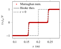
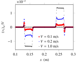
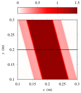
Figures 2 and 3 illustrate the coupling between plane shear waves and plane compression waves in hyperelasticity [9, 23], contrary to linear elasticity where both types of waves are decoupled. Fig. 2 displays a map of W1/8superscript𝑊18W^{1/8} at t=0.015𝑡0.015t=0.015 ms, where W𝑊W is the strain energy (6) obtained numerically with the above method. Fig. 3 display the evolution of the rotated longitudinal velocity (v1)φ=v1cosφ+v2sinφsubscriptsubscript𝑣1𝜑subscript𝑣1𝜑subscript𝑣2𝜑(v_{1})_{\varphi}=v_{1}\cos\varphi+v_{2}\sin\varphi and the rotated transverse velocity (v2)φ=v1sinφ+v2cosφsubscriptsubscript𝑣2𝜑subscript𝑣1𝜑subscript𝑣2𝜑(v_{2})_{\varphi}=-v_{1}\sin\varphi+v_{2}\cos\varphi, along the solid line displayed in Fig. 2. In the case of Hooke’s law of linear elasticity, the solution to the initial-value problem (27) writes

𝐪(x,y,t)={V(0,0,0,0,sinφ,cosφ,0)ifxφ<cSt,VcS(sinφcosφ,sin2φ,cos2φ,sinφcosφ,0,0,0)ifcSt<xφ<cSt,V(0,0,0,0,sinφ,cosφ,0)ifcSt<xφ,\mathbf{q}(x,y,t)=\left\{{\begin{aligned} V\,&\big{(}0,0,0,0,\phantom{-\!}\sin\varphi,-\!\cos\varphi,0\big{)}^{\top}&&\text{if}\;x_{\varphi}<-c_{S}t\,,\\ \frac{V}{c_{S}}\,&\big{(}\!-\!\sin\varphi\cos\varphi,-\!\sin^{2}\!\varphi,\cos^{2}\!\varphi,\sin\varphi\cos\varphi,0,0,0\big{)}^{\top}&&\text{if}\;{-c_{S}}t<x_{\varphi}<c_{S}t\,,\\ V\,&\big{(}0,0,0,0,-\!\sin\varphi,\phantom{-\!}\cos\varphi,0\big{)}^{\top}&&\text{if}\;c_{S}t<x_{\varphi}\,,\end{aligned}}\right. (28)

with cS=μ/ρ0subscript𝑐𝑆𝜇subscript𝜌0c_{S}=\sqrt{\mu/\rho_{0}}\,, and only shear waves propagate (solid line in Fig. 3). In the hyperelastic case, Fig. 3b shows that shear waves are generated from the initial data (27), but faster compression waves are also generated. This amplitude-dependent nonlinear effect is better observed at large amplitudes. The small-amplitude perturbations in the numerical solution are caused by the discretization of the oblique discontinuity (27).
Refer to caption
Figure 2: Generation of compression waves from pure shear initial data in Murnaghan hyperelasticity (g0𝑔0g\equiv 0). Map of W1/8superscript𝑊18W^{1/8} at t=0.015𝑡0.015t=0.015 ms, where W𝑊W is the strain energy density (J/m3) deduced from the numerical solution. The velocity amplitude of the impact problem (27) is V=0.1𝑉0.1V=0.1 m/s.

(a)

Refer to caption

(b)

Refer to caption
Figure 3: Rotated longitudinal and transverse velocities (v1)φsubscriptsubscript𝑣1𝜑(v_{1})_{\varphi}, (v2)φsubscriptsubscript𝑣2𝜑(v_{2})_{\varphi} along the line y=0.2𝑦0.2y=0.2 m in Fig. 2. (a) Normalized velocity (v2)φ/Vsubscriptsubscript𝑣2𝜑𝑉(v_{2})_{\varphi}/V in the linear and nonlinear cases for V=0.1𝑉0.1V=0.1 m/s. (b) Normalized velocity (v1)φ/Vsubscriptsubscript𝑣1𝜑𝑉(v_{1})_{\varphi}/V in the nonlinear case for various amplitudes V𝑉V.

4.2 Softening

In this second example, we consider the full system (15)-(16). The material is initially undeformed and at rest, 𝐪(x,y,0)=𝟎𝐪𝑥𝑦00\mathbf{q}(x,y,0)=\mathbf{0}, and a volume force 𝒇vsuperscript𝒇𝑣\bm{f}^{v} is used for the forcing 𝐬𝐬\mathbf{s}. The volume force is an acoustic point source along x𝑥x with expression 𝒇v=Avsin(2πfct)δ(xxs)δ(yys)𝒆1superscript𝒇𝑣superscript𝐴𝑣2𝜋subscript𝑓𝑐𝑡𝛿𝑥subscript𝑥𝑠𝛿𝑦subscript𝑦𝑠subscript𝒆1\bm{f}^{v}=A^{v}\sin(2\pi f_{c}t)\,\delta(x-x_{s})\,\delta(y-y_{s})\,\bm{e}_{1}, where δ𝛿\delta is the Dirac delta function, Avsuperscript𝐴𝑣A^{v} is the amplitude, and fcsubscript𝑓𝑐f_{c} is the characteristic frequency. Usually, the increment 𝐬i,jnsuperscriptsubscript𝐬𝑖𝑗𝑛\mathbf{s}_{i,j}^{n} in (19) is obtained by averaging the source term 𝐬|t=tnevaluated-at𝐬𝑡subscript𝑡𝑛\mathbf{s}|_{t=t_{n}} of (15)-(16) over the cell [xi1/2,xi+1/2]×[yj1/2,yj+1/2]subscript𝑥𝑖12subscript𝑥𝑖12subscript𝑦𝑗12subscript𝑦𝑗12[x_{i-1/2},x_{i+1/2}]\times[y_{j-1/2},y_{j+1/2}]. Here, we approximate the Dirac deltas by a truncated Gaussian function to avoid strain concentration at the source. Thus,

𝐬i,jn=Avρ0sin(2πfctn)exp((dij/σc)2)πσc2(1exp((R/σc)2))𝟏dijR(0,0,0,0,1,0,0),superscriptsubscript𝐬𝑖𝑗𝑛superscript𝐴𝑣subscript𝜌02𝜋subscript𝑓𝑐subscript𝑡𝑛superscriptsubscript𝑑𝑖𝑗subscript𝜎𝑐2𝜋superscriptsubscript𝜎𝑐21superscript𝑅subscript𝜎𝑐2subscript1subscript𝑑𝑖𝑗𝑅superscript0000100top\mathbf{s}_{i,j}^{n}=\frac{A^{v}}{\rho_{0}}\sin(2\pi f_{c}t_{n})\,\frac{\exp\big{(}{-(d_{ij}/\sigma_{c})^{2}}\big{)}}{\pi{\sigma_{c}}^{2}\left(1-\exp\big{(}{-(R/\sigma_{c})^{2}}\big{)}\right)}\mathbf{1}_{d_{ij}\leqslant R}\;(0,0,0,0,1,0,0)^{\top}, (29)

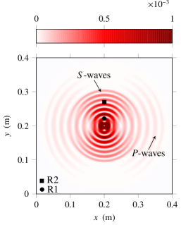
where dijsubscript𝑑𝑖𝑗d_{ij} is the distance between (xi,yj)subscript𝑥𝑖subscript𝑦𝑗(x_{i},y_{j}) and (xs,ys)subscript𝑥𝑠subscript𝑦𝑠(x_{s},y_{s}). Denoted by the indicator function 𝟏dijRsubscript1subscript𝑑𝑖𝑗𝑅\mathbf{1}_{d_{ij}\leqslant R}, the function’s support is a disk with radius R=cP/(7.5fc)𝑅subscript𝑐𝑃7.5subscript𝑓𝑐R=c_{P}/(7.5\,f_{c}), where cP=(λ+2μ)/ρ0subscript𝑐𝑃𝜆2𝜇subscript𝜌0c_{P}=\sqrt{(\lambda+2\mu)/\rho_{0}} is the speed of linear compression waves. The width parameter of the Gaussian function is chosen such that σc=R/2subscript𝜎𝑐𝑅2\sigma_{c}=R/2. The point load has amplitude Av=0.5superscript𝐴𝑣0.5A^{v}=0.5 kN/m, frequency fc=100subscript𝑓𝑐100f_{c}=100 kHz, and it is located at the nearest grid node of the domain’s center: (xs,ys)(Lx,Ly)/2similar-to-or-equalssubscript𝑥𝑠subscript𝑦𝑠subscript𝐿𝑥subscript𝐿𝑦2(x_{s},y_{s})\simeq(L_{x},L_{y})/2. The source (29) is switched on at t=0𝑡0t=0, and switched off at t=0.04𝑡0.04t=0.04 ms. Two receivers R1-R2 record the numerical solution during the simulation. R1 is located at (xr,yr)=(0.2,0.22)subscript𝑥𝑟subscript𝑦𝑟0.20.22(x_{r},y_{r})=(0.2,0.22) m, and R2 is located at (xr,yr)=(0.2,0.27)subscript𝑥𝑟subscript𝑦𝑟0.20.27(x_{r},y_{r})=(0.2,0.27) m.

(a)

Refer to caption

(b)

Refer to captionRefer to caption

(c)

Refer to captionRefer to caption
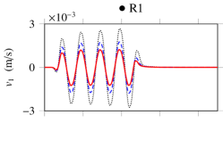
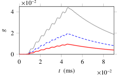
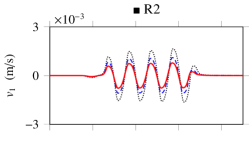
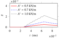
Figure 4: Softening induced by an acoustic point source (29). (a) Map of the strain energy (1g)W1𝑔𝑊\left(1-g\right)W in J/m3 at t=0.04𝑡0.04t=0.04 ms, where the forcing amplitude is Av=0.5superscript𝐴𝑣0.5A^{v}=0.5 kN/m. (b)-(c) Time histories of the velocity component v1subscript𝑣1v_{1} at the position of the receivers R1-R2 (bullet point and square on the map) for several forcing amplitudes (top); Same for the softening variable g𝑔g (bottom).

Figure 4 illustrates the effect of the softening on the wave propagation. Fig. 4a displays a map of the strain energy (1g)W1𝑔𝑊\left(1-g\right)W at the time t=0.04𝑡0.04t=0.04 ms, which shows the propagation of cylindrical waves. Denoted by a bullet point and by a square, the receivers R1-R2 are located in a region of the plane where mainly shear waves propagate. Figs. 4b-4c show the effect of the softening at the position of the receivers for several forcing amplitudes Avsuperscript𝐴𝑣A^{v}. One observes that g𝑔g increases while the wave passes by the receiver, and that it relaxes towards zero afterwards. This softening/recovery process is all the more important as the forcing amplitude is large. The characteristic time of the slow dynamics τ1/γ0.05subscript𝜏1𝛾0.05\tau_{1}/\gamma\approx 0.05 ms corresponds to the characteristic time of the recovery [16, 17]. In Figs. 4b-4c, one observes the distortion of the velocity signal during propagation, and its delay due to the increase of g𝑔g. The recorded signals are similar to experimental ones obtained in a longitudinal configuration [24].

4.3 Periodic layered medium

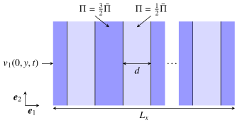
Similarly to [25, 26, 27], a periodic layered medium is considered. The basis vector 𝒆1subscript𝒆1\bm{e}_{1} which orientates the x𝑥x-axis is normal to the interfaces. The layers have the same thickness d=1𝑑1d=1 cm and perfect contact is assumed between neighbor layers (continuity of the displacement and of the stress). As illustrated in Fig. 5, the linear material properties Π{ρ0,λ,μ}Πsubscript𝜌0𝜆𝜇\Pi\in\{\rho_{0},\lambda,\mu\} vary in space according to

Π(x,y)={32Π¯ifx/d+0.50(mod 2),12Π¯otherwise,\Pi(x,y)=\left\{\begin{aligned} &\textstyle\frac{3}{2}\bar{\Pi}&&\text{if}\quad\lfloor x/d+0.5\rfloor\equiv 0\;(\text{mod}\;2),\\ &\textstyle\frac{1}{2}\bar{\Pi}&&\text{otherwise},\end{aligned}\right. (30)

where Π¯{ρ¯0,λ¯,μ¯}¯Πsubscript¯𝜌0¯𝜆¯𝜇\bar{\Pi}\in\{\bar{\rho}_{0},\bar{\lambda},\bar{\mu}\} denotes the reference parameters given in Table 1. The nonlinear material properties 𝔩𝔩\mathfrak{l}, 𝔪𝔪\mathfrak{m}, γ𝛾\gamma, τ1subscript𝜏1\tau_{1} do not vary in space. A velocity pulse with frequency fc=10subscript𝑓𝑐10f_{c}=10 kHz and amplitude V=1𝑉1V=1 m/s is imposed at the boundary x=0𝑥0x=0:

v1(0,y,t)=Vsin(πfct)2 10t1/fc.v_{1}(0,y,t)=V\sin(\pi f_{c}t)^{2}\,{\bf 1}_{0\leqslant t\leqslant 1/f_{c}}\,. (31)

Since the configuration is invariant along y𝑦y, the problem is one-dimensional. The wavelength of compression waves cPeff/fc39cmdsuperscriptsubscript𝑐𝑃effsubscript𝑓𝑐39cmmuch-greater-than𝑑c_{P}^{\text{eff}}/f_{c}\approx 39~{}\text{cm}\gg d is deduced from the effective sound speed

cPeff=32λ¯+2μ¯ρ¯03861m/ssuperscriptsubscript𝑐𝑃eff32¯𝜆2¯𝜇subscript¯𝜌03861m/sc_{P}^{\text{eff}}=\frac{\sqrt{3}}{2}\sqrt{\frac{\bar{\lambda}+2\bar{\mu}}{\bar{\rho}_{0}}}\approx 3861~{}\text{m/s} (32)

in the linear layered medium.

Refer to caption
Figure 5: Map of the periodic medium’s linear material properties Π{ρ0,λ,μ}Πsubscript𝜌0𝜆𝜇\Pi\in\{\rho_{0},\lambda,\mu\} over the numerical domain, where Π¯{ρ¯0,λ¯,μ¯}¯Πsubscript¯𝜌0¯𝜆¯𝜇\bar{\Pi}\in\{\bar{\rho}_{0},\bar{\lambda},\bar{\mu}\} denotes the reference values from Table 1.

The numerical domain defined by Lx=1subscript𝐿𝑥1L_{x}=1 m is discretized using Nx=3000subscript𝑁𝑥3000N_{x}=3000 points, i.e. each layer is represented by 30 points. The boundary condition (31) is implemented accordingly to Sec. 7.3.4 of [18] up to t=1/fc𝑡1subscript𝑓𝑐t=1/f_{c}. For t>1/fc𝑡1subscript𝑓𝑐t>1/f_{c}, periodic boundary conditions are applied (see Sec. 7.1 of [18]). A modification of the numerical method described in Sec. 3 is introduced to account for spatially-varying coefficients (B).

Figure 6 illustrates the effect of spatially-varying coefficients on the numerical solution up to t=2.5𝑡2.5t=2.5 ms. Figs. 6a-6b display seismograms obtained by unwrapping the velocity signals v1(0,y,t)subscript𝑣10𝑦𝑡v_{1}(0,y,t) recorded at the abscissa x=0𝑥0x=0. The “offset” corresponds to the effective propagation distance from the abscissa x=0𝑥0x=0 where the source (31) is imposed. Fig. 6a is obtained with the Murnaghan parameters 𝔩𝔩\mathfrak{l}, 𝔪𝔪\mathfrak{m} in Table 1 while the softening variable g𝑔g is equal to zero (no softening: τ1+subscript𝜏1\tau_{1}\to{+\infty}). Wavefront steepening is observed, leading to a series of oscillations. Fig. 6b shows the same output when the softening variable g𝑔g evolves according to (8), with the parameters γ=105𝛾superscript105\gamma=10^{5} Jm3Jsuperscriptm3\text{J}\,\text{m}^{-3} and τ1=5.0subscript𝜏15.0\tau_{1}=5.0 Jm3sJsuperscriptm3s\text{J}\,\text{m}^{-3}\,\text{s}. The parameters γ𝛾\gamma, τ1subscript𝜏1\tau_{1} are chosen such that the variable g𝑔g reaches values of 3% during the simulation, while the characteristic time τ1/γ=5×105subscript𝜏1𝛾5superscript105\tau_{1}/\gamma=5\times 10^{-5} s is the same as in Table 1. With respect to the case without softening (Fig. 6a), a longer propagation distance is needed until the wave separates into a series of oscillations, and the amplitudes of oscillations are modified.

(a)

Refer to caption

(b)

Refer to caption

(c)

Refer to caption
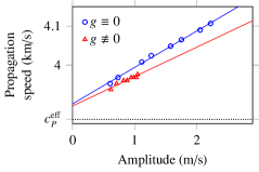
Figure 6: (a) Seismograms of the particle velocity v1subscript𝑣1v_{1} for a propagating sinusoidal pulse in a periodic layered Murnaghan material (g0𝑔0g\equiv 0). (b) Same output in the case of a periodic layered material with softening (g0not-equivalent-to𝑔0g\not\equiv 0). (c) In each case, we represent the observed speed of the largest oscillations over the range of propagation distances [6,8]68[6,8] m with respect to their amplitude at the propagation distance 777 m.

The speed of the largest oscillations over the range of propagation distances [6,8]68[6,8] m is deduced from Figs. 6a-6b and reported in Fig. 6c, where the abscissa is the amplitude of each oscillation at the propagation distance 777 m. This procedure is repeated with a smaller input amplitude V=0.9𝑉0.9V=0.9 m/s. A nearly linear evolution of the propagation speed with respect to the amplitude is observed, as is the case for solitary waves. At small amplitudes, the propagation speed is close to the effective speed of sound cPeffsuperscriptsubscript𝑐𝑃effc_{P}^{\text{eff}} (32). Similar observations are reported in [27] where a different constitutive law is used. Numerically, Fig. 6c shows that the softening does not suppress the solitary waves, but it modifies the relationship between their amplitude and their propagation speed.

5 Conclusion

Within the Lagrangian finite-strain theory, the constitutive model used in this study expresses the stress as a function of the Green–Lagrange strain tensor and a softening variable g𝑔g. Also, an evolution equation for g𝑔g is provided. The system of partial differential equations so-obtained writes as a nonlinear hyperbolic system of balance laws, so that finite-volume methods can be applied. If the softening is neglected, then the material follows Murnaghan’s law, where a shear wave excitation induces the propagation of smaller-amplitude compression waves. Otherwise, the propagation of a perturbation is responsible for the softening of the material, which recovers gradually its initial stiffness after excitation has stopped. Several numerical examples are considered along the paper. The latter have been chosen to serve modeling purposes rather than experimental ones, related to the observation of hysteresis and long-time relaxation in geophysics and non-destructive testing. In a periodic layered medium, solitary waves are numerically observed, as known in the case of nonlinear elastodynamics.

Now, let us mention possible future works. In the Lagrangian plane-strain case, the numerical method presented here can be used for various hyperelastic constitutive models, such as neo-Hookean, Mooney–Rivlin, Ogden, etc. [7, 8]. For such models, it would be interesting to solve analytically the symmetric shear impact problem in Fig. 2 for validation purposes. Variations of the evolution equation of g𝑔g in (8) can be considered as well. The influence of the softening on the smoothness of solutions could be investigated numerically and theoretically. To go further towards realistic configurations, viscoelastic attenuation should be accounted for, e.g. in a similar fashion to [28]. Concerning the nonlinear layered medium, it would be interesting to derive the corresponding nonlinear dispersive wave equations by homogenization, as done in [29, 27, 30] and related works. For the development of higher-order methods such as ENO or WENO schemes [31], the eigendecomposition of the fluxes provided in the A is a useful result.

Acknowledgments

This work was supported by the interdisciplinary mission of CNRS (INFINITI). The project leading to this publication has received funding from Excellence Initiative of Aix-Marseille University - A*MIDEX, a French “Investissements d’Avenir” programme. It has been carried out in the framework of the Labex MEC. Opération réalisée avec le concours du Programme d’investissements d’avenir du Gouvernement français dont la gestion a été confiée à l’Andra.

Appendix A Jacobian matrices of the flux

A.1 Expression of the coefficients

We use the Einstein summation convention with indices in {1,2}12\{1,2\}. To encompass both cases with and without geometric nonlinearity in a single equation, we introduce a parameter Θ{0,1}Θ01\Theta\in\{0,1\} such that Θ=1Θ1\Theta=1 corresponds to finite strain and Θ=0Θ0\Theta=0 corresponds to infinitesimal strain. Hence, the coordinates of the strain tensor (4) are written Eij=εij+12Θup,iup,jsubscript𝐸𝑖𝑗subscript𝜀𝑖𝑗12Θsubscript𝑢𝑝𝑖subscript𝑢𝑝𝑗E_{ij}=\varepsilon_{ij}+\frac{1}{2}\Theta\,u_{p,i}u_{p,j}, where εij=12(ui,j+uj,i)subscript𝜀𝑖𝑗12subscript𝑢𝑖𝑗subscript𝑢𝑗𝑖\varepsilon_{ij}=\frac{1}{2}(u_{i,j}+u_{j,i}) are the coordinates of the infinitesimal strain tensor. Moreover, the components of the Piola–Kirchhoff stress tensor (14) are written Pij=(1g)(δim+Θui,m)(α~0δmj+α~1Emj)subscript𝑃𝑖𝑗1𝑔subscript𝛿𝑖𝑚Θsubscript𝑢𝑖𝑚subscript~𝛼0subscript𝛿𝑚𝑗subscript~𝛼1subscript𝐸𝑚𝑗P_{ij}=(1-g)\left(\delta_{im}+\Theta\,u_{i,m}\right)\big{(}\tilde{\alpha}_{0}\delta_{mj}+\tilde{\alpha}_{1}E_{mj}\big{)}, i.e.

Pij=(1g)(α~0δij+α~1Eij+Θ(α~0ui,j+α~1ui,mEmj)),subscript𝑃𝑖𝑗1𝑔subscript~𝛼0subscript𝛿𝑖𝑗subscript~𝛼1subscript𝐸𝑖𝑗Θsubscript~𝛼0subscript𝑢𝑖𝑗subscript~𝛼1subscript𝑢𝑖𝑚subscript𝐸𝑚𝑗P_{ij}=(1-g)\left(\tilde{\alpha}_{0}\delta_{ij}+\tilde{\alpha}_{1}E_{ij}+\Theta\left(\tilde{\alpha}_{0}u_{i,j}+\tilde{\alpha}_{1}u_{i,m}E_{mj}\right)\right), (33)

where α~0subscript~𝛼0\tilde{\alpha}_{0}, α~1subscript~𝛼1\tilde{\alpha}_{1} are given in (13). The coefficients (17) of the Jacobian matrices 𝐟(𝐪)superscript𝐟𝐪\mathbf{f}^{\prime}(\mathbf{q}) and 𝐠(𝐪)superscript𝐠𝐪\mathbf{g}^{\prime}(\mathbf{q}) satisfy ρ0Qijk=Pij/uk,subscript𝜌0subscript𝑄𝑖𝑗𝑘subscript𝑃𝑖𝑗subscript𝑢𝑘\rho_{0}Q_{ijk\ell}=\partial P_{ij}/\partial u_{k,\ell} and ρ0Gij=Pij/gsubscript𝜌0subscript𝐺𝑖𝑗subscript𝑃𝑖𝑗𝑔\rho_{0}G_{ij}=\partial P_{ij}/\partial g. In the present case of Murnaghan material with softening (33), one has

ρ0Qijksubscript𝜌0subscript𝑄𝑖𝑗𝑘\displaystyle\rho_{0}Q_{ijk\ell} =(1g)(δijα~0uk,+Eijα~1uk,+α~1Eijuk,)absent1𝑔subscript𝛿𝑖𝑗subscript~𝛼0subscript𝑢𝑘subscript𝐸𝑖𝑗subscript~𝛼1subscript𝑢𝑘subscript~𝛼1subscript𝐸𝑖𝑗subscript𝑢𝑘\displaystyle=(1-g)\left(\delta_{ij}\frac{\partial\tilde{\alpha}_{0}}{\partial u_{k,\ell}}+E_{ij}\frac{\partial\tilde{\alpha}_{1}}{\partial u_{k,\ell}}+\tilde{\alpha}_{1}\frac{\partial E_{ij}}{\partial u_{k,\ell}}\right) (34)
+Θ(1g)(ui,jα~0uk,+α~0δikδj+ui,mEmjα~1uk,+α~1(δikEj+ui,mEmjuk,)),Θ1𝑔subscript𝑢𝑖𝑗subscript~𝛼0subscript𝑢𝑘subscript~𝛼0subscript𝛿𝑖𝑘subscript𝛿𝑗subscript𝑢𝑖𝑚subscript𝐸𝑚𝑗subscript~𝛼1subscript𝑢𝑘subscript~𝛼1subscript𝛿𝑖𝑘subscript𝐸𝑗subscript𝑢𝑖𝑚subscript𝐸𝑚𝑗subscript𝑢𝑘\displaystyle+\Theta\,(1-g)\left(u_{i,j}\frac{\partial\tilde{\alpha}_{0}}{\partial u_{k,\ell}}+\tilde{\alpha}_{0}\delta_{ik}\delta_{j\ell}+u_{i,m}E_{mj}\frac{\partial\tilde{\alpha}_{1}}{\partial u_{k,\ell}}+\tilde{\alpha}_{1}\left(\delta_{ik}E_{j\ell}+u_{i,m}\frac{\partial E_{mj}}{\partial u_{k,\ell}}\right)\right),
ρ0Gijsubscript𝜌0subscript𝐺𝑖𝑗\displaystyle\rho_{0}G_{ij} =(α~0δij+α~1Eij+Θ(α~0ui,j+α~1ui,mEmj)),absentsubscript~𝛼0subscript𝛿𝑖𝑗subscript~𝛼1subscript𝐸𝑖𝑗Θsubscript~𝛼0subscript𝑢𝑖𝑗subscript~𝛼1subscript𝑢𝑖𝑚subscript𝐸𝑚𝑗\displaystyle=-\left(\tilde{\alpha}_{0}\delta_{ij}+\tilde{\alpha}_{1}E_{ij}+\Theta\left(\tilde{\alpha}_{0}u_{i,j}+\tilde{\alpha}_{1}u_{i,m}E_{mj}\right)\right),

where

Eijuk,subscript𝐸𝑖𝑗subscript𝑢𝑘\displaystyle\frac{\partial E_{ij}}{\partial u_{k,\ell}} =12(δikδj+δjkδi)+12Θ(uk,iδj+uk,jδi),absent12subscript𝛿𝑖𝑘subscript𝛿𝑗subscript𝛿𝑗𝑘subscript𝛿𝑖12Θsubscript𝑢𝑘𝑖subscript𝛿𝑗subscript𝑢𝑘𝑗subscript𝛿𝑖\displaystyle=\frac{1}{2}\big{(}\delta_{ik}\delta_{j\ell}+\delta_{jk}\delta_{i\ell}\big{)}+\frac{1}{2}\Theta\,\big{(}u_{k,i}\delta_{j\ell}+u_{k,j}\delta_{i\ell}\big{)}\,, Ennuk,subscript𝐸𝑛𝑛subscript𝑢𝑘\displaystyle\frac{\partial E_{nn}}{\partial u_{k,\ell}} =δk+Θuk,,absentsubscript𝛿𝑘Θsubscript𝑢𝑘\displaystyle=\delta_{k\ell}+\Theta\,u_{k,\ell}\,,
α~0uk,subscript~𝛼0subscript𝑢𝑘\displaystyle\frac{\partial\tilde{\alpha}_{0}}{\partial u_{k,\ell}} =(λ+2(𝔩𝔪)Emm)Ennuk,+2𝔪EijEijuk,,absent𝜆2𝔩𝔪subscript𝐸𝑚𝑚subscript𝐸𝑛𝑛subscript𝑢𝑘2𝔪subscript𝐸𝑖𝑗subscript𝐸𝑖𝑗subscript𝑢𝑘\displaystyle=\left(\lambda+2(\mathfrak{l}-\mathfrak{m})E_{mm}\right)\frac{\partial E_{nn}}{\partial u_{k,\ell}}+2\mathfrak{m}E_{ij}\frac{\partial E_{ij}}{\partial u_{k,\ell}}\,,
α~1uk,subscript~𝛼1subscript𝑢𝑘\displaystyle\frac{\partial\tilde{\alpha}_{1}}{\partial u_{k,\ell}} =2𝔪Ennuk,.absent2𝔪subscript𝐸𝑛𝑛subscript𝑢𝑘\displaystyle=2\mathfrak{m}\frac{\partial E_{nn}}{\partial u_{k,\ell}}\,.

The case of Hookean solids is recovered if g0𝑔0g\equiv 0, geometric nonlinearity is neglected (Θ=0Θ0\Theta=0), and the Murnaghan coefficients 𝔩𝔩\mathfrak{l}, 𝔪𝔪\mathfrak{m} are zero. In this case, Eq. (34) gives ρ0Qijk=λδijδk+μ(δikδj+δjkδi)subscript𝜌0subscript𝑄𝑖𝑗𝑘𝜆subscript𝛿𝑖𝑗subscript𝛿𝑘𝜇subscript𝛿𝑖𝑘subscript𝛿𝑗subscript𝛿𝑗𝑘subscript𝛿𝑖\rho_{0}Q_{ijk\ell}=\lambda\delta_{ij}\delta_{k\ell}+\mu(\delta_{ik}\delta_{j\ell}+\delta_{jk}\delta_{i\ell}).

A.2 Eigendecomposition

We provide an eigendecomposition of the Jacobian matrices 𝐟(𝐪)superscript𝐟𝐪\mathbf{f}^{\prime}(\mathbf{q}) and 𝐠(𝐪)superscript𝐠𝐪\mathbf{g}^{\prime}(\mathbf{q}) of the fluxes. The hyperelastic case without softening is recovered by removing the last row and the last column of each matrix in the following paragraphs.

Flux along the x𝑥x-axis

The Jacobian matrix (17) of 𝐟𝐟\mathbf{f} at the linear average (23) is diagonalized. Let us write 𝐀i+1/2,j=𝐏𝚲𝐏1subscript𝐀𝑖12𝑗𝐏𝚲superscript𝐏1\mathbf{A}_{i+1/2,j}=\mathbf{P}\mathbf{\Lambda}\mathbf{P}^{-1} where 𝐏𝐏\mathbf{P} is an invertible real matrix, and 𝚲𝚲\mathbf{\Lambda} is a diagonal real matrix. The matrix of eigenvalues 𝚲=diag(cP,cP,cS,cS,0,0,0)𝚲diagsubscript𝑐𝑃subscript𝑐𝑃subscript𝑐𝑆subscript𝑐𝑆000\mathbf{\Lambda}=\text{diag}(-c_{P},c_{P},-c_{S},c_{S},0,0,0) satisfies

cP,S=12Q1111+Q2121±(Q1111Q2121)2+4Q1121Q2111,subscript𝑐𝑃𝑆12plus-or-minussubscript𝑄1111subscript𝑄2121superscriptsubscript𝑄1111subscript𝑄212124subscript𝑄1121subscript𝑄2111c_{P,S}=\frac{1}{\sqrt{2}}\sqrt{Q_{1111}+Q_{2121}\pm\sqrt{\left(Q_{1111}-Q_{2121}\right)^{2}+4\,Q_{1121}Q_{2111}}\,}\;, (35)

where the plus sign gives the expression of cPsubscript𝑐𝑃c_{P} (compressional waves), and the minus sign gives the expression of cSsubscript𝑐𝑆c_{S} (shear waves). The first four right eigenvectors 𝐩i+1/2,jksubscriptsuperscript𝐩𝑘𝑖12𝑗\mathbf{p}^{k}_{i+1/2,j} of 𝐀i+1/2,jsubscript𝐀𝑖12𝑗\mathbf{A}_{i+1/2,j} used in (24)-(25) are the first four columns of 𝐏𝐏\mathbf{P}, where

𝐏=(p11p11p13p13p15p16p170000p25p26p27p31p31p33p33100000001011p13/p33p13/p33000p31/p11p31/p11110000000001),𝐏matrixsubscript𝑝11subscript𝑝11subscript𝑝13subscript𝑝13subscript𝑝15subscript𝑝16subscript𝑝170000subscript𝑝25subscript𝑝26subscript𝑝27subscript𝑝31subscript𝑝31subscript𝑝33subscript𝑝33100000001011subscript𝑝13subscript𝑝33subscript𝑝13subscript𝑝33000subscript𝑝31subscript𝑝11subscript𝑝31subscript𝑝11110000000001\mathbf{P}={\begin{pmatrix}p_{11}&-p_{11}&p_{13}&-p_{13}&p_{15}&p_{16}&p_{17}\\ 0&0&0&0&p_{25}&p_{26}&p_{27}\\ p_{31}&-p_{31}&p_{33}&-p_{33}&1&0&0\\ 0&0&0&0&0&1&0\\ 1&1&p_{13}/p_{33}&p_{13}/p_{33}&0&0&0\\ p_{31}/p_{11}&p_{31}/p_{11}&1&1&0&0&0\\ 0&0&0&0&0&0&1\end{pmatrix}}\,, (36)

with the coefficients

p11subscript𝑝11\displaystyle p_{11} =1/cP,absent1subscript𝑐𝑃\displaystyle={1}/{c_{P}}\,, p31subscript𝑝31\displaystyle p_{31} =Q2111/cP(cP)2Q2121,absentsubscript𝑄2111subscript𝑐𝑃superscriptsubscript𝑐𝑃2subscript𝑄2121\displaystyle=\frac{Q_{2111}/c_{P}}{(c_{P})^{2}-Q_{2121}}\,,
p13subscript𝑝13\displaystyle p_{13} =(cP)2Q1121/cS((cP)2Q2121)Q1111+Q1121Q2111,absentsuperscriptsubscript𝑐𝑃2subscript𝑄1121subscript𝑐𝑆superscriptsubscript𝑐𝑃2subscript𝑄2121subscript𝑄1111subscript𝑄1121subscript𝑄2111\displaystyle=-\frac{(c_{P})^{2}\,Q_{1121}/c_{S}}{\left((c_{P})^{2}-Q_{2121}\right)Q_{1111}+Q_{1121}Q_{2111}}\,, p33subscript𝑝33\displaystyle p_{33} =1/cS,absent1subscript𝑐𝑆\displaystyle={1}/{c_{S}}\,,
p15subscript𝑝15\displaystyle p_{15} =Q1112Q2121Q1121Q2112Q1111Q2112Q1112Q2111,absentsubscript𝑄1112subscript𝑄2121subscript𝑄1121subscript𝑄2112subscript𝑄1111subscript𝑄2112subscript𝑄1112subscript𝑄2111\displaystyle=\frac{Q_{1112}Q_{2121}-Q_{1121}Q_{2112}}{Q_{1111}Q_{2112}-Q_{1112}Q_{2111}}\,, p25subscript𝑝25\displaystyle p_{25} =Q1121Q2111Q1111Q2121Q1111Q2112Q1112Q2111,absentsubscript𝑄1121subscript𝑄2111subscript𝑄1111subscript𝑄2121subscript𝑄1111subscript𝑄2112subscript𝑄1112subscript𝑄2111\displaystyle=\frac{Q_{1121}Q_{2111}-Q_{1111}Q_{2121}}{Q_{1111}Q_{2112}-Q_{1112}Q_{2111}}\,,
p16subscript𝑝16\displaystyle p_{16} =Q1112Q2122Q1122Q2112Q1111Q2112Q1112Q2111,absentsubscript𝑄1112subscript𝑄2122subscript𝑄1122subscript𝑄2112subscript𝑄1111subscript𝑄2112subscript𝑄1112subscript𝑄2111\displaystyle=\frac{Q_{1112}Q_{2122}-Q_{1122}Q_{2112}}{Q_{1111}Q_{2112}-Q_{1112}Q_{2111}}\,, p26subscript𝑝26\displaystyle p_{26} =Q1122Q2111Q1111Q2122Q1111Q2112Q1112Q2111,absentsubscript𝑄1122subscript𝑄2111subscript𝑄1111subscript𝑄2122subscript𝑄1111subscript𝑄2112subscript𝑄1112subscript𝑄2111\displaystyle=\frac{Q_{1122}Q_{2111}-Q_{1111}Q_{2122}}{Q_{1111}Q_{2112}-Q_{1112}Q_{2111}}\,,
p17subscript𝑝17\displaystyle p_{17} =G21Q1112G11Q2112Q1111Q2112Q1112Q2111,absentsubscript𝐺21subscript𝑄1112subscript𝐺11subscript𝑄2112subscript𝑄1111subscript𝑄2112subscript𝑄1112subscript𝑄2111\displaystyle=\frac{G_{21}Q_{1112}-G_{11}Q_{2112}}{Q_{1111}Q_{2112}-Q_{1112}Q_{2111}}\,, p27subscript𝑝27\displaystyle p_{27} =G11Q2111G21Q1111Q1111Q2112Q1112Q2111.absentsubscript𝐺11subscript𝑄2111subscript𝐺21subscript𝑄1111subscript𝑄1111subscript𝑄2112subscript𝑄1112subscript𝑄2111\displaystyle=\frac{G_{11}Q_{2111}-G_{21}Q_{1111}}{Q_{1111}Q_{2112}-Q_{1112}Q_{2111}}\,.

The matrix 𝐏𝐏\mathbf{P} is invertible provided that its determinant is nonzero, i.e. Q1121Q2111Q1111Q2121subscript𝑄1121subscript𝑄2111subscript𝑄1111subscript𝑄2121Q_{1121}Q_{2111}\neq Q_{1111}Q_{2121} and Q1121Q211114(Q1111Q2121)2subscript𝑄1121subscript𝑄211114superscriptsubscript𝑄1111subscript𝑄21212Q_{1121}Q_{2111}\neq-\frac{1}{4}(Q_{1111}-Q_{2121})^{2}. Let us consider each equality case:

  • 1.

    if Q1121Q2111=Q1111Q2121subscript𝑄1121subscript𝑄2111subscript𝑄1111subscript𝑄2121Q_{1121}Q_{2111}=Q_{1111}Q_{2121}, then the eigenvalues of 𝐟(𝐪)superscript𝐟𝐪\mathbf{f}^{\prime}(\mathbf{q}) satisfy cS=0subscript𝑐𝑆0c_{S}=0. Therefore, the reduced system of conservation laws for plane waves propagating along x𝑥x is not strictly hyperbolic (eigenvalues {cP,cP,cS,cS,0}subscript𝑐𝑃subscript𝑐𝑃subscript𝑐𝑆subscript𝑐𝑆0\{{-c_{P},c_{P},-c_{S},c_{S},0}\});

  • 2.

    if Q1121Q2111=14(Q1111Q2121)2subscript𝑄1121subscript𝑄211114superscriptsubscript𝑄1111subscript𝑄21212Q_{1121}Q_{2111}=-\frac{1}{4}(Q_{1111}-Q_{2121})^{2}, then the eigenvalues of 𝐟(𝐪)superscript𝐟𝐪\mathbf{f}^{\prime}(\mathbf{q}) satisfy cP=cSsubscript𝑐𝑃subscript𝑐𝑆c_{P}=c_{S}, which is impossible for the same reason.

Therefore, the previous eigendecomposition is valid over the domain of strict hyperbolicity. The first four left eigenvectors 𝐥i+1/2,jksuperscriptsubscript𝐥𝑖12𝑗𝑘\mathbf{l}_{i+1/2,j}^{k} of 𝐀i+1/2,jsubscript𝐀𝑖12𝑗\mathbf{A}_{i+1/2,j} are the first four rows of 𝐏1superscript𝐏1\mathbf{P}^{-1}, where

𝐏1=(q11q12q13q14q15q16q17q11q12q13q14q15q16q17q41q42q43q44q45q46q47q41q42q43q44q45q46q4701/p250p26/p2500p27/p2500010000000001),superscript𝐏1matrixsubscript𝑞11subscript𝑞12subscript𝑞13subscript𝑞14subscript𝑞15subscript𝑞16subscript𝑞17subscript𝑞11subscript𝑞12subscript𝑞13subscript𝑞14subscript𝑞15subscript𝑞16subscript𝑞17subscript𝑞41subscript𝑞42subscript𝑞43subscript𝑞44subscript𝑞45subscript𝑞46subscript𝑞47subscript𝑞41subscript𝑞42subscript𝑞43subscript𝑞44subscript𝑞45subscript𝑞46subscript𝑞4701subscript𝑝250subscript𝑝26subscript𝑝2500subscript𝑝27subscript𝑝2500010000000001\mathbf{P}^{-1}={\begin{pmatrix}q_{11}&q_{12}&q_{13}&q_{14}&q_{15}&q_{16}&q_{17}\\ -q_{11}&-q_{12}&-q_{13}&-q_{14}&q_{15}&q_{16}&-q_{17}\\ -q_{41}&-q_{42}&-q_{43}&-q_{44}&q_{45}&q_{46}&-q_{47}\\ q_{41}&q_{42}&q_{43}&q_{44}&q_{45}&q_{46}&q_{47}\\ 0&1/p_{25}&0&-p_{26}/p_{25}&0&0&-p_{27}/p_{25}\\ 0&0&0&1&0&0&0\\ 0&0&0&0&0&0&1\end{pmatrix}}\,, (37)

with the coefficients

q11subscript𝑞11\displaystyle q_{11} =12p33p11p33p13p31,absent12subscript𝑝33subscript𝑝11subscript𝑝33subscript𝑝13subscript𝑝31\displaystyle=\frac{1}{2}{\frac{p_{33}}{p_{11}p_{33}-p_{13}p_{31}}}\,, q41subscript𝑞41\displaystyle q_{41} =12p31p11p33p13p31,absent12subscript𝑝31subscript𝑝11subscript𝑝33subscript𝑝13subscript𝑝31\displaystyle=\frac{1}{2}{\frac{p_{31}}{p_{11}p_{33}-p_{13}p_{31}}}\,,
q12subscript𝑞12\displaystyle q_{12} =12p13p15p33p25(p11p33p13p31),absent12subscript𝑝13subscript𝑝15subscript𝑝33subscript𝑝25subscript𝑝11subscript𝑝33subscript𝑝13subscript𝑝31\displaystyle=\frac{1}{2}{\frac{p_{13}-p_{15}p_{33}}{p_{25}\left(p_{11}p_{33}-p_{13}p_{31}\right)}}\,, q42subscript𝑞42\displaystyle q_{42} =12p11p15p31p25(p11p33p13p31),absent12subscript𝑝11subscript𝑝15subscript𝑝31subscript𝑝25subscript𝑝11subscript𝑝33subscript𝑝13subscript𝑝31\displaystyle=\frac{1}{2}{\frac{p_{11}-p_{15}p_{31}}{p_{25}\left(p_{11}p_{33}-p_{13}p_{31}\right)}}\,,
q13subscript𝑞13\displaystyle q_{13} =12p13p11p33p13p31,absent12subscript𝑝13subscript𝑝11subscript𝑝33subscript𝑝13subscript𝑝31\displaystyle=-\frac{1}{2}{\frac{p_{13}}{p_{11}p_{33}-p_{13}p_{31}}}\,, q43subscript𝑞43\displaystyle q_{43} =12p11p11p33p13p31,absent12subscript𝑝11subscript𝑝11subscript𝑝33subscript𝑝13subscript𝑝31\displaystyle=-\frac{1}{2}{\frac{p_{11}}{p_{11}p_{33}-p_{13}p_{31}}}\,,
q14subscript𝑞14\displaystyle q_{14} =12(p15p26p16p25)p33p13p26p25(p11p33p13p31),absent12subscript𝑝15subscript𝑝26subscript𝑝16subscript𝑝25subscript𝑝33subscript𝑝13subscript𝑝26subscript𝑝25subscript𝑝11subscript𝑝33subscript𝑝13subscript𝑝31\displaystyle=\frac{1}{2}{\frac{\left(p_{15}p_{26}-p_{16}p_{25}\right)p_{33}-p_{13}p_{26}}{p_{25}\left(p_{11}p_{33}-p_{13}p_{31}\right)}}\,, q44subscript𝑞44\displaystyle q_{44} =12(p15p26p16p25)p31p11p26p25(p11p33p13p31),absent12subscript𝑝15subscript𝑝26subscript𝑝16subscript𝑝25subscript𝑝31subscript𝑝11subscript𝑝26subscript𝑝25subscript𝑝11subscript𝑝33subscript𝑝13subscript𝑝31\displaystyle=\frac{1}{2}{\frac{\left(p_{15}p_{26}-p_{16}p_{25}\right)p_{31}-p_{11}p_{26}}{p_{25}\left(p_{11}p_{33}-p_{13}p_{31}\right)}}\,,
q15subscript𝑞15\displaystyle q_{15} =12p11p33p11p33p13p31,absent12subscript𝑝11subscript𝑝33subscript𝑝11subscript𝑝33subscript𝑝13subscript𝑝31\displaystyle=\frac{1}{2}{\frac{p_{11}p_{33}}{p_{11}p_{33}-p_{13}p_{31}}}\,, q45subscript𝑞45\displaystyle q_{45} =12p31p33p11p33p13p31,absent12subscript𝑝31subscript𝑝33subscript𝑝11subscript𝑝33subscript𝑝13subscript𝑝31\displaystyle=-\frac{1}{2}{\frac{p_{31}p_{33}}{p_{11}p_{33}-p_{13}p_{31}}}\,,
q16subscript𝑞16\displaystyle q_{16} =12p13p11p11p33p13p31,absent12subscript𝑝13subscript𝑝11subscript𝑝11subscript𝑝33subscript𝑝13subscript𝑝31\displaystyle=-\frac{1}{2}{\frac{p_{13}p_{11}}{p_{11}p_{33}-p_{13}p_{31}}}\,, q46subscript𝑞46\displaystyle q_{46} =12p11p33p11p33p13p31,absent12subscript𝑝11subscript𝑝33subscript𝑝11subscript𝑝33subscript𝑝13subscript𝑝31\displaystyle=\frac{1}{2}{\frac{p_{11}p_{33}}{p_{11}p_{33}-p_{13}p_{31}}}\,,
q17subscript𝑞17\displaystyle q_{17} =12(p15p27p17p25)p33p13p27p25(p11p33p13p31),absent12subscript𝑝15subscript𝑝27subscript𝑝17subscript𝑝25subscript𝑝33subscript𝑝13subscript𝑝27subscript𝑝25subscript𝑝11subscript𝑝33subscript𝑝13subscript𝑝31\displaystyle=\frac{1}{2}\frac{\left(p_{15}p_{27}-p_{17}p_{25}\right)p_{33}-p_{13}p_{27}}{p_{25}\left(p_{11}p_{33}-p_{13}p_{31}\right)}\,, q47subscript𝑞47\displaystyle q_{47} =12(p15p27p17p25)p31p11p27p25(p11p33p13p31).absent12subscript𝑝15subscript𝑝27subscript𝑝17subscript𝑝25subscript𝑝31subscript𝑝11subscript𝑝27subscript𝑝25subscript𝑝11subscript𝑝33subscript𝑝13subscript𝑝31\displaystyle=\frac{1}{2}{\frac{\left(p_{15}p_{27}-p_{17}p_{25}\right)p_{31}-p_{11}p_{27}}{p_{25}\left(p_{11}p_{33}-p_{13}p_{31}\right)}}\,.

The coefficients αi+1/2,jksubscriptsuperscript𝛼𝑘𝑖12𝑗\alpha^{k}_{i+1/2,j} in (24) are equal to the scalar products αi+1/2,jk=𝐥i+1/2,jk(𝐪i+1,jn𝐪i,jn)subscriptsuperscript𝛼𝑘𝑖12𝑗subscriptsuperscript𝐥𝑘𝑖12𝑗superscriptsubscript𝐪𝑖1𝑗𝑛superscriptsubscript𝐪𝑖𝑗𝑛\alpha^{k}_{i+1/2,j}=\mathbf{l}^{k}_{i+1/2,j}\cdot\left(\mathbf{q}_{i+1,j}^{n}-\mathbf{q}_{i,j}^{n}\right).

Flux along the y𝑦y-axis

Similarly to (23), we introduce the Jacobian matrix 𝐠(𝐪)superscript𝐠𝐪\mathbf{g}^{\prime}(\mathbf{q}) of 𝐠𝐠\mathbf{g} at the linear average 𝐁i,j+1/2=𝐠(12(𝐪i,jn+𝐪i,j+1n))subscript𝐁𝑖𝑗12superscript𝐠12superscriptsubscript𝐪𝑖𝑗𝑛superscriptsubscript𝐪𝑖𝑗1𝑛\mathbf{B}_{i,j+1/2}=\mathbf{g}^{\prime}\left(\frac{1}{2}(\mathbf{q}_{i,j}^{n}+\mathbf{q}_{i,j+1}^{n})\right), and provide an eigendecomposition 𝐁i,j+1/2=𝐏𝚲𝐏1subscript𝐁𝑖𝑗12𝐏𝚲superscript𝐏1\mathbf{B}_{i,j+1/2}=\mathbf{P}\mathbf{\Lambda}\mathbf{P}^{-1}. The matrix of eigenvalues 𝚲=diag(cP,cP,cS,cS,0,0,0)𝚲diagsubscript𝑐𝑃subscript𝑐𝑃subscript𝑐𝑆subscript𝑐𝑆000\mathbf{\Lambda}=\text{diag}(-c_{P},c_{P},-c_{S},c_{S},0,0,0) satisfies

cP,S=12Q2222+Q1212±(Q2222Q1212)2+4Q2212Q1222,subscript𝑐𝑃𝑆12plus-or-minussubscript𝑄2222subscript𝑄1212superscriptsubscript𝑄2222subscript𝑄121224subscript𝑄2212subscript𝑄1222c_{P,S}=\frac{1}{\sqrt{2}}\sqrt{Q_{2222}+Q_{1212}\pm\sqrt{\left(Q_{2222}-Q_{1212}\right)^{2}+4\,Q_{2212}Q_{1222}}\,}\;, (38)

where the plus and minus signs give the expressions of cPsubscript𝑐𝑃c_{P} and cSsubscript𝑐𝑆c_{S}, respectively. With similar notations as (36), we have

𝐏=(0000p15p16p17p21p21p23p23p25p26p270000010p41p41p43p43100p21/p41p21/p411100011p43/p23p43/p230000000001),𝐏matrix0000subscript𝑝15subscript𝑝16subscript𝑝17subscript𝑝21subscript𝑝21subscript𝑝23subscript𝑝23subscript𝑝25subscript𝑝26subscript𝑝270000010subscript𝑝41subscript𝑝41subscript𝑝43subscript𝑝43100subscript𝑝21subscript𝑝41subscript𝑝21subscript𝑝411100011subscript𝑝43subscript𝑝23subscript𝑝43subscript𝑝230000000001\mathbf{P}={\begin{pmatrix}0&0&0&0&p_{15}&p_{16}&p_{17}\\ p_{21}&-p_{21}&p_{23}&-p_{23}&p_{25}&p_{26}&p_{27}\\ 0&0&0&0&0&1&0\\ p_{41}&-p_{41}&p_{43}&-p_{43}&1&0&0\\ p_{21}/p_{41}&p_{21}/p_{41}&1&1&0&0&0\\ 1&1&p_{43}/p_{23}&p_{43}/p_{23}&0&0&0\\ 0&0&0&0&0&0&1\end{pmatrix}}\,, (39)

with the coefficients

p21subscript𝑝21\displaystyle p_{21} =(cS)2Q1222/cP((cP)2Q1212)Q1212Q1222Q2212,absentsuperscriptsubscript𝑐𝑆2subscript𝑄1222subscript𝑐𝑃superscriptsubscript𝑐𝑃2subscript𝑄1212subscript𝑄1212subscript𝑄1222subscript𝑄2212\displaystyle=\frac{(c_{S})^{2}\,Q_{1222}/c_{P}}{\left((c_{P})^{2}-Q_{1212}\right)Q_{1212}-Q_{1222}Q_{2212}}\,, p41subscript𝑝41\displaystyle p_{41} =1/cP,absent1subscript𝑐𝑃\displaystyle=1/c_{P}\,,
p23subscript𝑝23\displaystyle p_{23} =1/cS,absent1subscript𝑐𝑆\displaystyle=1/c_{S}\,, p43subscript𝑝43\displaystyle p_{43} =Q2212/cS(cP)2Q1212,absentsubscript𝑄2212subscript𝑐𝑆superscriptsubscript𝑐𝑃2subscript𝑄1212\displaystyle=-\frac{Q_{2212}/c_{S}}{(c_{P})^{2}-Q_{1212}}\,,
p15subscript𝑝15\displaystyle p_{15} =Q1212Q2222Q1222Q2212Q1211Q2212Q1212Q2211,absentsubscript𝑄1212subscript𝑄2222subscript𝑄1222subscript𝑄2212subscript𝑄1211subscript𝑄2212subscript𝑄1212subscript𝑄2211\displaystyle=\frac{Q_{1212}Q_{2222}-Q_{1222}Q_{2212}}{Q_{1211}Q_{2212}-Q_{1212}Q_{2211}}\,, p25subscript𝑝25\displaystyle p_{25} =Q1222Q2211Q1211Q2222Q1211Q2212Q1212Q2211,absentsubscript𝑄1222subscript𝑄2211subscript𝑄1211subscript𝑄2222subscript𝑄1211subscript𝑄2212subscript𝑄1212subscript𝑄2211\displaystyle=\frac{Q_{1222}Q_{2211}-Q_{1211}Q_{2222}}{Q_{1211}Q_{2212}-Q_{1212}Q_{2211}}\,,
p16subscript𝑝16\displaystyle p_{16} =Q1212Q2221Q1221Q2212Q1211Q2212Q1212Q2211,absentsubscript𝑄1212subscript𝑄2221subscript𝑄1221subscript𝑄2212subscript𝑄1211subscript𝑄2212subscript𝑄1212subscript𝑄2211\displaystyle=\frac{Q_{1212}Q_{2221}-Q_{1221}Q_{2212}}{Q_{1211}Q_{2212}-Q_{1212}Q_{2211}}\,, p26subscript𝑝26\displaystyle p_{26} =Q1221Q2211Q1211Q2221Q1211Q2212Q1212Q2211,absentsubscript𝑄1221subscript𝑄2211subscript𝑄1211subscript𝑄2221subscript𝑄1211subscript𝑄2212subscript𝑄1212subscript𝑄2211\displaystyle=\frac{Q_{1221}Q_{2211}-Q_{1211}Q_{2221}}{Q_{1211}Q_{2212}-Q_{1212}Q_{2211}}\,,
p17subscript𝑝17\displaystyle p_{17} =G22Q1212G12Q2212Q1211Q2212Q1212Q2211,absentsubscript𝐺22subscript𝑄1212subscript𝐺12subscript𝑄2212subscript𝑄1211subscript𝑄2212subscript𝑄1212subscript𝑄2211\displaystyle=\frac{G_{22}Q_{1212}-G_{12}Q_{2212}}{Q_{1211}Q_{2212}-Q_{1212}Q_{2211}}\,, p27subscript𝑝27\displaystyle p_{27} =G12Q2211G22Q1211Q1211Q2212Q1212Q2211.absentsubscript𝐺12subscript𝑄2211subscript𝐺22subscript𝑄1211subscript𝑄1211subscript𝑄2212subscript𝑄1212subscript𝑄2211\displaystyle=\frac{G_{12}Q_{2211}-G_{22}Q_{1211}}{Q_{1211}Q_{2212}-Q_{1212}Q_{2211}}\,.

A similar analysis shows that 𝐏𝐏\mathbf{P} is invertible over the domain of strict hyperbolicity:

𝐏1=(q11q12q13q14q15q16q17q11q12q13q14q15q16q17q41q42q43q44q45q46q47q41q42q43q44q45q46q471/p250p16/p15000p17/p1500100000000001),superscript𝐏1matrixsubscript𝑞11subscript𝑞12subscript𝑞13subscript𝑞14subscript𝑞15subscript𝑞16subscript𝑞17subscript𝑞11subscript𝑞12subscript𝑞13subscript𝑞14subscript𝑞15subscript𝑞16subscript𝑞17subscript𝑞41subscript𝑞42subscript𝑞43subscript𝑞44subscript𝑞45subscript𝑞46subscript𝑞47subscript𝑞41subscript𝑞42subscript𝑞43subscript𝑞44subscript𝑞45subscript𝑞46subscript𝑞471subscript𝑝250subscript𝑝16subscript𝑝15000subscript𝑝17subscript𝑝1500100000000001\mathbf{P}^{-1}={\begin{pmatrix}q_{11}&q_{12}&q_{13}&q_{14}&q_{15}&q_{16}&q_{17}\\ -q_{11}&-q_{12}&-q_{13}&-q_{14}&q_{15}&q_{16}&-q_{17}\\ -q_{41}&-q_{42}&-q_{43}&-q_{44}&q_{45}&q_{46}&-q_{47}\\ q_{41}&q_{42}&q_{43}&q_{44}&q_{45}&q_{46}&q_{47}\\ 1/p_{25}&0&-p_{16}/p_{15}&0&0&0&-p_{17}/p_{15}\\ 0&0&1&0&0&0&0\\ 0&0&0&0&0&0&1\end{pmatrix}}\,, (40)

with the coefficients

q11subscript𝑞11\displaystyle q_{11} =12p23p25p43p15(p21p43p23p41),absent12subscript𝑝23subscript𝑝25subscript𝑝43subscript𝑝15subscript𝑝21subscript𝑝43subscript𝑝23subscript𝑝41\displaystyle=\frac{1}{2}{\frac{p_{23}-p_{25}p_{43}}{p_{15}\left(p_{21}p_{43}-p_{23}p_{41}\right)}}\,, q41subscript𝑞41\displaystyle q_{41} =12p21p25p41p15(p21p43p23p41),absent12subscript𝑝21subscript𝑝25subscript𝑝41subscript𝑝15subscript𝑝21subscript𝑝43subscript𝑝23subscript𝑝41\displaystyle=\frac{1}{2}{\frac{p_{21}-p_{25}p_{41}}{p_{15}\left(p_{21}p_{43}-p_{23}p_{41}\right)}}\,,
q12subscript𝑞12\displaystyle q_{12} =12p43p21p43p23p41,absent12subscript𝑝43subscript𝑝21subscript𝑝43subscript𝑝23subscript𝑝41\displaystyle=\frac{1}{2}{\frac{p_{43}}{p_{21}p_{43}-p_{23}p_{41}}}\,, q42subscript𝑞42\displaystyle q_{42} =12p41p21p43p23p41,absent12subscript𝑝41subscript𝑝21subscript𝑝43subscript𝑝23subscript𝑝41\displaystyle=\frac{1}{2}{\frac{p_{41}}{p_{21}p_{43}-p_{23}p_{41}}}\,,
q13subscript𝑞13\displaystyle q_{13} =12(p16p25p15p26)p43p16p23p15(p21p43p23p41),absent12subscript𝑝16subscript𝑝25subscript𝑝15subscript𝑝26subscript𝑝43subscript𝑝16subscript𝑝23subscript𝑝15subscript𝑝21subscript𝑝43subscript𝑝23subscript𝑝41\displaystyle=\frac{1}{2}{\frac{\left(p_{16}p_{25}-p_{15}p_{26}\right)p_{43}-p_{16}p_{23}}{p_{15}\left(p_{21}p_{43}-p_{23}p_{41}\right)}}\,, q43subscript𝑞43\displaystyle q_{43} =12(p16p25p15p26)p41p16p21p15(p21p43p23p41),absent12subscript𝑝16subscript𝑝25subscript𝑝15subscript𝑝26subscript𝑝41subscript𝑝16subscript𝑝21subscript𝑝15subscript𝑝21subscript𝑝43subscript𝑝23subscript𝑝41\displaystyle=\frac{1}{2}{\frac{\left(p_{16}p_{25}-p_{15}p_{26}\right)p_{41}-p_{16}p_{21}}{p_{15}\left(p_{21}p_{43}-p_{23}p_{41}\right)}}\,,
q14subscript𝑞14\displaystyle q_{14} =12p23p21p43p23p41,absent12subscript𝑝23subscript𝑝21subscript𝑝43subscript𝑝23subscript𝑝41\displaystyle=-\frac{1}{2}{\frac{p_{23}}{p_{21}p_{43}-p_{23}p_{41}}}\,, q44subscript𝑞44\displaystyle q_{44} =12p21p21p43p23p41,absent12subscript𝑝21subscript𝑝21subscript𝑝43subscript𝑝23subscript𝑝41\displaystyle=-\frac{1}{2}{\frac{p_{21}}{p_{21}p_{43}-p_{23}p_{41}}}\,,
q15subscript𝑞15\displaystyle q_{15} =12p43p41p21p43p23p41,absent12subscript𝑝43subscript𝑝41subscript𝑝21subscript𝑝43subscript𝑝23subscript𝑝41\displaystyle=\frac{1}{2}{\frac{p_{43}p_{41}}{p_{21}p_{43}-p_{23}p_{41}}}\,, q45subscript𝑞45\displaystyle q_{45} =12p41p23p21p43p23p41,absent12subscript𝑝41subscript𝑝23subscript𝑝21subscript𝑝43subscript𝑝23subscript𝑝41\displaystyle=-\frac{1}{2}{\frac{p_{41}p_{23}}{p_{21}p_{43}-p_{23}p_{41}}}\,,
q16subscript𝑞16\displaystyle q_{16} =12p41p23p21p43p23p41,absent12subscript𝑝41subscript𝑝23subscript𝑝21subscript𝑝43subscript𝑝23subscript𝑝41\displaystyle=-\frac{1}{2}{\frac{p_{41}p_{23}}{p_{21}p_{43}-p_{23}p_{41}}}\,, q46subscript𝑞46\displaystyle q_{46} =12p23p21p21p43p23p41,absent12subscript𝑝23subscript𝑝21subscript𝑝21subscript𝑝43subscript𝑝23subscript𝑝41\displaystyle=\frac{1}{2}{\frac{p_{23}p_{21}}{p_{21}p_{43}-p_{23}p_{41}}}\,,
q17subscript𝑞17\displaystyle q_{17} =12(p17p25p15p27)p43p17p23p15(p21p43p23p41),absent12subscript𝑝17subscript𝑝25subscript𝑝15subscript𝑝27subscript𝑝43subscript𝑝17subscript𝑝23subscript𝑝15subscript𝑝21subscript𝑝43subscript𝑝23subscript𝑝41\displaystyle=\frac{1}{2}{\frac{\left(p_{17}p_{25}-p_{15}p_{27}\right)p_{43}-p_{17}p_{23}}{p_{15}\left(p_{21}p_{43}-p_{23}p_{41}\right)}}\,, q47subscript𝑞47\displaystyle q_{47} =12(p17p25p15p27)p41p17p21p15(p21p43p23p41).absent12subscript𝑝17subscript𝑝25subscript𝑝15subscript𝑝27subscript𝑝41subscript𝑝17subscript𝑝21subscript𝑝15subscript𝑝21subscript𝑝43subscript𝑝23subscript𝑝41\displaystyle=\frac{1}{2}{\frac{\left(p_{17}p_{25}-p_{15}p_{27}\right)p_{41}-p_{17}p_{21}}{p_{15}\left(p_{21}p_{43}-p_{23}p_{41}\right)}}\,.

Appendix B Spatially-varying coefficients

The problem described in Fig. 5 is one-dimensional. Thus, the variable y𝑦y and the index j𝑗j do not appear in the present description of the numerical method, which is a modification of (25) to account for spatially-varying coefficients [25, 26, 27] (cf. Chap. 9 of [18]). The conservation laws (15) are rewritten in terms of 𝐪=(u1,1,ρ0v1,g)𝐪superscriptsubscript𝑢11subscript𝜌0subscript𝑣1𝑔top{\bf q}=(u_{1,1},\rho_{0}v_{1},g)^{\top}\!. The modified method amounts to choosing the eigenvalues {cP,cP,0}subscript𝑐𝑃subscript𝑐𝑃0\{{-c_{P}},c_{P},0\} and corresponding eigenvectors 𝐩i+1/2,jksuperscriptsubscript𝐩𝑖12𝑗𝑘{\bf p}_{i+1/2,j}^{k}, k{1,3}𝑘13k\in\{1,3\} of 𝐀i+1/2subscript𝐀𝑖12{\bf A}_{i+1/2} in a downwind fashion. Hence, cPsubscript𝑐𝑃c_{P} is computed at the abscissa xisubscript𝑥𝑖x_{i} for k=1𝑘1k=1 and at the abscissa xi+1subscript𝑥𝑖1x_{i+1} for k=2𝑘2k=2. Since both left-going and right-going waves do not have equal absolute speeds at the cell interface xi+1/2subscript𝑥𝑖12x_{i+1/2}, writing the low-order part of the algorithm (25) as a flux difference is no longer possible: the “wave-propagation form” is used instead. To guarantee the continuity of the velocity and of the stress at the material interfaces, a modified expression of the coefficients αi+1/2ksubscriptsuperscript𝛼𝑘𝑖12\alpha^{k}_{i+1/2} defining the vectors 𝓦i+1/2ksubscriptsuperscript𝓦𝑘𝑖12\bm{\mathcal{W}}^{k}_{i+1/2} is used. In particular, the sum of these vectors does not equal the jump 𝐪i+1𝐪isubscript𝐪𝑖1subscript𝐪𝑖{\bf q}_{i+1}-{\bf q}_{i} anymore, as was the case in a homogeneous medium (24). To avoid numerical instability, a transmission-based limiter is implemented, which modifies the expression (26) of the coefficients θi+1/2ksubscriptsuperscript𝜃𝑘𝑖12\theta^{k}_{i+1/2}.

References

  • [1] P. A. Johnson, B. Zinszner, P. N. J. Rasolofosaon, Resonance and elastic nonlinear phenomena in rock, J. Geophys. Res.-Sol. Ea. 101 (B5) (1996) 11553–11564.
  • [2] M. C. Remillieux, R. A. Guyer, C. Payan, T. J. Ulrich, Decoupling nonclassical nonlinear behavior of elastic wave types, Phys. Rev. Lett. 116 (11) (2016) 115501.
  • [3] J. A. Ten Cate, T. J. Shankland, Slow dynamics in the nonlinear elastic response of berea sandstone, Geophys. Res. Lett. 23 (21) (1996) 3019–3022.
  • [4] J. A. TenCate, Slow dynamics of earth materials: An experimental overview, Pure Appl. Geophys. 168 (12) (2011) 2211–2219.
  • [5] J. Rivière, G. Renaud, R. A. Guyer, P. A. Johnson, Pump and probe waves in dynamic acousto-elasticity: Comprehensive description and comparison with nonlinear elastic theories, J. Appl. Phys. 114 (5) (2013) 054905.
  • [6] S. Haupert, G. Renaud, J. Rivière, P. Shokouhi, Dynamic acousto-elastic testing, in: T. Kundu (Ed.), Nonlinear Ultrasonic and Vibro-Acoustical Techniques for Nondestructive Evaluation, Springer, 2019, Ch. 13, pp. 509–546.
  • [7] R. W. Ogden, Non-linear Elastic Deformations, Ellis Harwood Ltd., 1984.
  • [8] G. A. Holzapfel, Nonlinear Solid Mechanics: A Continuum Approach for Engineering, John Wiley & Sons Ltd., 2000.
  • [9] A. N. Norris, Finite-amplitude waves in solids, in: M. F. Hamilton, D. T. Blackstock (Eds.), Nonlinear Acoustics, Academic press, 1998, Ch. 9, pp. 263–277.
  • [10] F. D. Murnaghan, Finite deformations of an elastic solid, Am. J. Math. 59 (2) (1937) 235–260.
  • [11] P. A. Johnson, P. N. J. Rasolofosaon, Nonlinear elasticity and stress-induced anisotropy in rock, J. Geophys. Res.-Sol. Ea. 101 (B2) (1996) 3113–3124.
  • [12] K. W. Winkler, X. Liu, Measurements of third-order elastic constants in rocks, J. Acoust. Soc. Am. 100 (3) (1996) 1392–1398.
  • [13] C. Payan, V. Garnier, J. Moysan, P. A. Johnson, Determination of third order elastic constants in a complex solid applying coda wave interferometry, Appl. Phys. Lett. 94 (2009) 011904.
  • [14] V. Lyakhovsky, Y. Ben-‐Zion, A. Agnon, Distributed damage, faulting, and friction, J. Geophys. Res.-Sol. Ea. 102 (B12) (1997) 27635–27649.
  • [15] O. O. Vakhnenko, V. O. Vakhnenko, T. J. Shankland, J. A. Ten Cate, Strain-induced kinetics of intergrain defects as the mechanism of slow dynamics in the nonlinear resonant response of humid sandstone bars, Phys. Rev. E 70 (1) (2004) 015602.
  • [16] H. Berjamin, N. Favrie, B. Lombard, G. Chiavassa, Nonlinear waves in solids with slow dynamics: an internal-variable model, Proc. R. Soc. A 473 (2201) (2017) 20170024.
  • [17] H. Berjamin, B. Lombard, G. Chiavassa, N. Favrie, A finite-volume approach to 1D nonlinear elastic waves: Application to slow dynamics, Acta Acust. united Ac. 104 (4) (2018) 561–570.
  • [18] R. J. LeVeque, Finite Volume Methods for Hyperbolic Problems, Cambridge University Press, 2002.
  • [19] O. Bou Matar, P.-Y. Guerder, Y. Li, B. Vandewoestyne, K. Van Den Abeele, A nodal discontinuous Galerkin finite element method for nonlinear elastic wave propagation, J. Acoust. Soc. Am. 131 (5) (2012) 3650–3663.
  • [20] D. S. Drumheller, Introduction to Wave Propagation in Nonlinear Fluids and Solids, Cambridge University Press, 1998.
  • [21] S. Ndanou, N. Favrie, S. Gavrilyuk, Criterion of hyperbolicity in hyperelasticity in the case of the stored energy in separable form, J. Elast. 115 (1) (2014) 1–25.
  • [22] G. Strang, Accurate partial difference methods I: Linear Cauchy problems, Arch. Ration. Mech. An. 12 (1) (1963) 392–402.
  • [23] N. Favrie, S. Gavrilyuk, S. Ndanou, A thermodynamically compatible splitting procedure in hyperelasticity, J. Comput. Phys. 270 (2014) 300–324.
  • [24] M. C. Remillieux, T. J. Ulrich, H. E. Goodman, J. A. Ten Cate, Propagation of a finite-amplitude elastic pulse in a bar of berea sandstone: A detailed look at the mechanisms of classical nonlinearity, hysteresis, and nonequilibrium dynamics, J. Geophys. Res.-Sol. Ea. 122 (11) (2017) 8892–8909.
  • [25] T. R. Fogarty, R. J. LeVeque, High-resolution finite-volume methods for acoustic waves in periodic and random media, J. Acoust. Soc. Am. 106 (1) (1999) 17–28.
  • [26] R. J. LeVeque, Finite-volume methods for non-linear elasticity in heterogeneous media, Int. J. Numer. Meth. Fluids 40 (1–2) (2002) 93–104.
  • [27] R. J. LeVeque, D. H. Yong, Solitary waves in layered nonlinear media, SIAM J. Appl. Math. 63 (5) (2003) 1539–1560.
  • [28] H. Berjamin, B. Lombard, G. Chiavassa, N. Favrie, Modeling longitudinal wave propagation in nonlinear viscoelastic solids with softening, Int. J. Solids Struct. 141–142 (2018) 35–44.
  • [29] A. M. Samsonov, Strain Solitons in Solids and How to Construct Them, Chapman and Hall/CRC, 2001.
  • [30] I. V. Andrianov, V. V. Danishevs’kyy, O. I. Ryzhkov, D. Weichert, Dynamic homogenization and wave propagation in a nonlinear 1D composite material, Wave Motion 50 (2) (2013) 271–281.
  • [31] C. W. Shu, High order weighted essentially nonoscillatory schemes for convection dominated problems, SIAM Rev. 51 (1) (2009) 82–126.