RINS-W: Robust Inertial Navigation System on Wheels

Abstract

This paper proposes a real-time approach for long-term inertial navigation based only on an Inertial Measurement Unit (IMU) for self-localizing wheeled robots. The approach builds upon two components: 1) a robust detector that uses recurrent deep neural networks to dynamically detect a variety of situations of interest, such as zero velocity or no lateral slip; and 2) a state-of-the-art Kalman filter which incorporates this knowledge as pseudo-measurements for localization. Evaluations on a publicly available car dataset demonstrates that the proposed scheme may achieve a final precision of 20 m for a 21 km long trajectory of a vehicle driving for over an hour, equipped with an IMU of moderate precision (the gyro drift rate is 10 deg/h). To our knowledge, this is the first paper which combines sophisticated deep learning techniques with state-of-the-art filtering methods for pure inertial navigation on wheeled vehicles and as such opens up for novel data-driven inertial navigation techniques. Moreover, albeit taylored for IMU-only based localization, our method may be used as a component for self-localization of wheeled robots equipped with a more complete sensor suite.

I Introduction

Inertial navigation, or “inertial odometry”, uses an Inertial Measurement Unit (IMU) consisting of accelerometers and gyrometers to calculate in real time by dead reckoning the position, the orientation, and the 3D velocity vector of a moving object without the need for external references or extra sensors. Albeit a mature field, the development of low-cost and small size inertial sensors over the past two decades has attracted much interest for robotics and autonomous systems applications, see e.g. [1, 2, 3].

High precision Inertial Navigation Systems (INS) achieve very small localization errors but are costly and rely on time-consuming initialization procedures [4]. In contrast, MEMS-based IMU suffer from large errors such as scale factor, axis misalignment, thermo-mechanical white noise and random walk noise, resulting in rapid localization drift. This prompts the need for fusion with complementary sensors such as GPS, cameras, or LiDAR, see e.g., [5, 6, 7].

In this paper, we provide a method for long-term localization for wheeled robots only using an IMU. Our contributions, and the paper’s organization, are as follows:

• we introduce specific motion profiles frequently encountered by a wheeled vehicle which bring information about the motion when correctly identified, along with their mathematical description in Section III;

• we design an algorithm which automatically detects in real time if any of those assumptions about the motion holds in Section IV-A, based only on the IMU measurements. The detector builds upon recurrent deep neural networks [8] and is trained using IMU and ground truth data;

• we implement a state-of-the-art invariant extended Kalman filter [9, 10] that exploits the detector’s outputs as pseudo-measurements to combine them with the IMU outputs in a statistical way, in Section IV-B. It yields accurate estimates of pose, velocity and sensor biases, along with associated uncertainty (covariance);

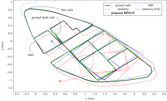
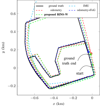
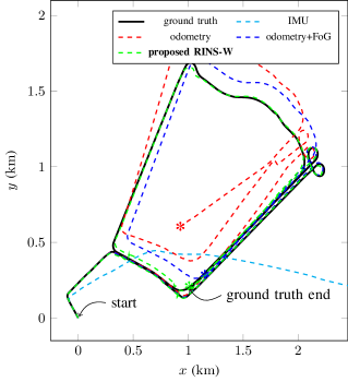
• we demonstrate the performances of the approach on a publicly available car dataset [11] in Section V. Our approach solely based on the IMU produces accurate estimates with a final distance w.r.t. ground truth of $20\text{\,}\mathrm{m}$ on the 73 minutes test sequence urban16, see Figure 1. In particular, our approach outperforms differential wheel odometry, as well as wheel odometry aided by an expensive fiber optics gyro whose drift is 200 times smaller than the one of the IMU we use;

• this evidences that accurately detecting some specific patterns in the IMU data and incorporating this information in a filter may prove very fruitful for localization;

• the method is not restricted to IMU only based navigation. It is possible to feed the Kalman filter with other sensors’ measurements. Besides, once trained the detector may be used as a building block in any localization algorithm.

Figure 1: Trajectory ground truth and estimates obtained by various methods: integration of IMU signals; odometry based on a differential wheel encoder system; odometry combined with an highly accurate and expensive Fiber optics Gyro (FoG) that provides orientation estimates; and the proposed RINS-W approach which considers only the IMU sensor embarked in the vehicle, and which outperforms the other schemes. The final distance error for this long-term sequence urban16 (73 minutes) of the car dataset [11] is $20\text{\,}\mathrm{m}$ for the RINS-W solution. The deep learning based detector (see Section IV-A) has of course not been trained or cross-validated on this sequence.

I-A Related Works

Odometry and localization based on inertial sensors, cameras, and/or LIDARs have made tremendous progresses over the last decade, enabling robust real-time localization systems, see e.g., [5, 6, 7]. As concerns back-end techniques, although optimization-based methods tend to presently prevail, filtering based methods building upon the Invariant Extended Kalman Filter (IEKF) [9, 10] are currently gaining interest, owing to its theoretical guarantees in terms of convergence and consistency. The IEKF [9] has already given rise to a commercial product in the field of high precision navigation, see [12, 10]. It has also been successfully applied to visual inertial odometry, in [13, 14, 15] and bipedal robotics [16].

Taking into account vehicle constraints and odometer measurements are known to increase the robustness of visual-inertial systems [17, 18]. Although quite successful, systems using vision continuously process a large amount of data which is computationally demanding and energy consuming. Moreover, an autonomous vehicle should run in parallel its own robust IMU-based localization algorithm to perform maneuvers such as emergency stops if LiDAR and camera are unavailable due to lack of texture or information, and more generally failures [1].

Inertial navigation systems have long leveraged pseudo-measurements from IMU signals, e.g. the widespread Zero velocity UPdaTe (ZUPT) [19, 20]. Upon detection of a zero-velocity event, such pseudo-measurement can be fused with the dead reckoning motion model in an extended Kalman filter [21, 22] or in a factor graph, see [23].

Very recently, great efforts have been devoted to the use of deep learning and more generally machine learning frameworks for pedestrian inertial navigation [24, 25, 26, 27, 28]. In [24] velocity is estimated using support vector regression whereas [25, 26, 27] use recurrent neural networks respectively for ZUPT detection, speed estimation, and end-to-end inertial navigation. Those methods are promising but difficult to transfer to a wheeled robots since they generally only consider horizontal planar motion, and must infer velocity directly from a small sequence of IMU measurements, whereas we can afford to use larger sequences. Finally, in [29], we used Gaussian Processes to learn and correct wheel encoders errors to improve wheel encoder based dead reckoning in 2D.

II Inertial Navigation System & Sensor Model

Denoting the IMU orientation by $\mathbf{R}_{n}\in SO(3)$, i.e. the rotation matrix that maps the body frame to the world frame w, its velocity in w by $\mathbf{v}_{n}^{\mathrm{\textsc{w}}}\in\mathbb{R}^{3}$ and its position in w by $\mathbf{p}_{n}^{\mathrm{\textsc{w}}}\in\mathbb{R}^{3}$, the dynamics are as follows

$$\mathbf{R}_{n+1} =\mathbf{R}_{n}\exp_{SO(3)}\left(\bm{\omega}_{n}dt\right),$$ (1)

$$\mathbf{v}_{n+1}^{\mathrm{\textsc{w}}} =\mathbf{v}_{n}^{\mathrm{\textsc{w}}}+\left(\mathbf{R}_{n}\mathbf{a}_{n}+\mathbf{g}\right)dt,$$ (2)

$$\mathbf{p}_{n+1}^{\mathrm{\textsc{w}}} =\mathbf{p}_{n}^{\mathrm{\textsc{w}}}+\mathbf{v}_{n}^{\mathrm{\textsc{w}}}dt,$$ (3)

between two discrete times, with sampling time $dt$, and where $\left(\mathbf{R}_{0},\mathbf{v}_{0}^{\mathrm{\textsc{w}}},\mathbf{p}_{0}^{\mathrm{\textsc{w}}}\right)$ is the initial configuration. The true angular velocity $\bm{\omega}_{n}\in\mathbb{R}^{3}$ and the true specific acceleration $\mathbf{a}_{n}\in\mathbb{R}^{3}$ are the inputs of the system (1)-(3). In our application scenarios, the effects of earth rotation and Coriolis acceleration are ignored, and earth is considered flat.

II-A Inertial Measurement Unit (IMU) Model

The IMU provides noisy and biased measurements of $\bm{\omega}_{n}\in\mathbb{R}^{3}$ and $\mathbf{a}_{n}\in\mathbb{R}^{3}$ as follows

$$\bm{\omega}_{n}^{\mathrm{\textsc{imu}}} =\bm{\omega}_{n}+\mathbf{b}_{n}^{\bm{\omega}}+\mathbf{w}_{n}^{\bm{\omega}},$$ (4)

$$\mathbf{a}^{\mathrm{\textsc{imu}}}_{n} =\mathbf{a}_{n}+\mathbf{b}_{n}^{\mathbf{a}}+\mathbf{w}_{n}^{\mathbf{a}},$$ (5)

where $\mathbf{b}_{n}^{\bm{\omega}}$, $\mathbf{b}_{n}^{\mathbf{a}}$ are quasi-constant biases and $\mathbf{w}_{n}^{\bm{\omega}}$, $\mathbf{w}_{n}^{\mathbf{a}}$ are zero-mean Gaussian noises. The biases follow a random-walk

$$\mathbf{b}_{n+1}^{\bm{\omega}} =\mathbf{b}_{n}^{\bm{\omega}}+\mathbf{w}^{\mathbf{b}_{\omega}}_{n},$$ (6)

$$\mathbf{b}_{n+1}^{\mathbf{a}} =\mathbf{b}_{n}^{\mathbf{a}}+\mathbf{w}^{\mathbf{b}_{\mathbf{a}}}_{n},$$ (7)

where $\mathbf{w}_{n}^{\mathbf{b}_{\bm{\omega}}}$, $\mathbf{w}^{\mathbf{b}_{\mathbf{a}}}_{n}$ are zero-mean Gaussian noises.

All sources of error - particularly biases - are yet undesirable since a simple implementation of (1)-(3) leads to a triple integration of raw data, which is much more harmful that the unique integration of differential wheel speeds. Even a small error may thus cause the position estimate to be way off the true position, within seconds.

III Specific Motion Profiles for Wheeled Systems

We describe in this section characteristic motions frequently encountered by a wheeled robot, that provide useful complementary information to the IMU when correctly detected.

III-A Considered Motion Profiles

We consider 4 distinct specific motion profiles, whose validity is encoded in the following binary vector:

$$\mathbf{z}_{n}=\left(z^{\mathrm{\textsc{vel}}}_{n},\leavevmode\nobreak\ z^{\mathrm{\textsc{ang}}}_{n},\leavevmode\nobreak\ z^{\mathrm{\textsc{lat}}}_{n},\leavevmode\nobreak\ z^{\mathrm{\textsc{up}}}_{n}\right)\in\{0,1\}^{4}.$$ (8)

• Zero velocity: the velocity of the platform is null. As a consequence so is the linear acceleration, yielding:

  $$z^{\mathrm{\textsc{vel}}}_{n}=1\Rightarrow\left\{\begin{matrix}\mathbf{v}_{n}=\mathbf{0}\\ \mathbf{R}_{n}\mathbf{a}_{n}+\mathbf{g}=\mathbf{0}\end{matrix}\right..$$ (9)

  Such profiles frequently occur for vehicles moving in urban environments, and are leveraged in the well known Zero velocity UPdaTe (ZUPT), see e.g. [19, 20].

• Zero angular velocity: the heading is constant:

  $$z^{\mathrm{\textsc{ang}}}_{n}=1\Rightarrow\bm{\omega}_{n}=\mathbf{0}.$$ (10)

• Zero lateral velocity: the lateral velocity is considered roughly null

  $$z^{\mathrm{\textsc{lat}}}_{n}=1\Rightarrow v_{n}^{\mathrm{\textsc{lat}}}\simeq 0,$$ (11)

  where we obtain the lateral velocity $v_{n}^{\mathrm{\textsc{lat}}}$ after expressing the velocity in the body frame b as

  $$\mathbf{v}_{n}^{\mathrm{\textsc{b}}}=\mathbf{R}_{n}^{T}\mathbf{v}_{n}^{\mathrm{\textsc{w}}}=\begin{bmatrix}v_{n}^{\mathrm{\textsc{for}}}\\ v_{n}^{\mathrm{\textsc{lat}}}\\ v_{n}^{\mathrm{\textsc{up}}}\end{bmatrix}.$$ (12)

• Zero vertical velocity: the vertical velocity is considered roughly null

  $$z^{\mathrm{\textsc{up}}}_{n}=1\Rightarrow v_{n}^{\mathrm{\textsc{up}}}\simeq 0.$$ (13)

The two latter are common assumptions for wheeled robots or cars moving forward on human made roads.

III-B Discussion on the Choice of Profiles

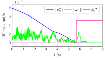
The motion profiles were carefully chosen in order to match the specificity of wheeled robots equipped with shock absorbers. Indeed, as illustrated on Figure 2, when the wheels of a car actually stop, the car undergoes a rotational motion forward and then backward. As a result, null velocity (9) does not imply null angular velocity (10). For the level of precision we pursue in the present paper, distinguishing between (9) and (10) is pivotal since it allows us to: $i$) properly label motion profiles before training (see Section V-B, where we have different thresholds on position and on angular velocity); and: $ii$) improve detection accuracy since only one motion pattern can be identified as valid.

Figure 2: Real IMU data of a car stopping from sequence urban06 of [11]. We see (9) holds and thus $z^{\mathrm{\textsc{vel}}}_{n}=1$ at $t=5.8s$ while (10) does not hold yet.

(11) and (13) generally hold for robots moving indoors or cars on roads. Note that (13) is expressed in the body frame, and thus generally holds for a car moving on a road even if the road is not level. As such (13) is more refined that just assuming the car is moving in a 2D horizontal plane. And it is actually quite a challenge for an IMU-based detector to identify when (11) and (13) are not valid.

III-C Expected Impacts on Robot Localization

The motion profiles fall into two categories in terms of the information they bring:

1. Zero velocity constraints: the profiles (9)-(10), when correctly detected may allow to correct the IMU biases, the pitch and the roll.

2. Vehicle motion constraints: the profiles (11) and (13) are useful constraints for the estimates accuracy over the long term. In particular, Section V-E will experimentally demonstrate the benefits of accounting for (11) and (13).

IV Proposed RINS-W Algorithm

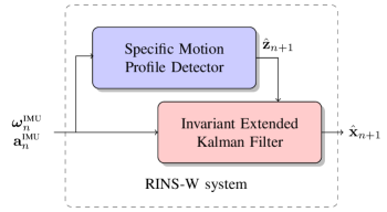
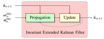
This section describes our system for recovering trajectory and sensor bias estimates from an IMU. Figure 3 illustrates the approach which consists of two main blocks summarized as follow:

• the detector estimates the binary vector $\mathbf{z}_{n}$ from raw IMU signals, and consists of recurrent neural networks;

• the filter integrates the IMU measurements in its dynamic model and exploits the detected motion profiles as pseudo-measurements to refine its estimates, as customary in inertial navigation, see e.g. [19].

The detector does not use the filter’s output and is based only on IMU measurements. Thus the detector operates autonomously and is trained independently, see Section V-B. Note that our approach is different from more tightly coupled approaches such as [30]. We now describe each block.

Figure 3: Structure of the proposed RINS-W system for inertial navigation. The detector identifies specific motion profiles (8) from raw IMU signals only.

IV-A The Specific Motion Profile Detector

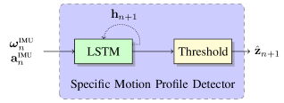
The detector determines at each instant $n$ which ones of the specific motion profiles (8) are valid, see Figure 4. The base core of the detector is a recurrent neural network, namely a Long-Short Term Memory (LSTM) [8]. The LSTMs take as input the IMU measurements and compute:

$$\hat{\mathbf{u}}_{n+1},\leavevmode\nobreak\ \mathbf{h}_{n+1} =\mathrm{LSTM}\left(\left\{\bm{\omega}^{\mathrm{\textsc{imu}}}_{i},\leavevmode\nobreak\ \mathbf{a}^{\mathrm{\textsc{imu}}}_{i}\right\}_{i=0}^{n}\right)$$ (14)

$$=\mathrm{LSTM}\left(\bm{\omega}^{\mathrm{\textsc{imu}}}_{n},\leavevmode\nobreak\ \mathbf{a}^{\mathrm{\textsc{imu}}}_{n},\leavevmode\nobreak\ \mathbf{h}_{n}\right),$$ (15)

where $\hat{\mathbf{u}}_{n+1}\in\mathbb{R}^{4}$ contains probability scores for each motion profiles and $\mathbf{h}_{n}$ is the hidden state of the neural network. Probability scores are then converted to a binary vector $\hat{\mathbf{z}}_{n}=\mathrm{Threshold}\left(\hat{\mathbf{u}}_{n+1}\right)$ with a threshold for each motion profile.

The thresholds must be set with care, and the procedure will be described in Section V-A. Indeed, false alarms lead to degraded performance, since a zero velocity assumption is incompatible with an actual motion. On the other hand, a missed profile is not harmful since it results in standard IMU based dead reckoning using (1)-(3).

Figure 4: Structure of the detector, which consists for each motion pattern of a recurrent neural network (LSTM) followed by a threshold to obtain an output vector $\hat{\mathbf{z}}_{n}$ that consists of binary components. The hidden state $\mathbf{h}_{n}$ of the neural network allows the full structure to be recursive.

IV-B The Invariant Extended Kalman Filter

The extended Kalman filter is the most widespread technique in the inertial navigation industry, since it was first successfully used in the Apollo program half a century ago. However, recent work advocates the use of a modified version, the Invariant Extended Kalman Filter (IEKF) [9] that has proved to bring drastic improvement over EKF, and has recently given raise to a commercial product, see [10, 12], and various successes in robotics [13, 15, 14, 16]. We thus opt for an IEKF to perform the fusion between the IMU measurements and the detected specific motion profiles. The IEKF outputs the state $\hat{\mathbf{x}}_{n}$ that consists of pose and velocity of the IMU, the IMU biases, along with their covariance. We now describe the filter more in detail, whose architecture is displayed on Figure 5.

Figure 5: Structure of the IEKF. The filter leverages motion profile information $\hat{\mathbf{z}}_{n}$ both for the propagation and the update of the state $\hat{\mathbf{x}}_{n+1}$.

IV-B1 IMU state

we define the IMU state as

$$\mathbf{x}_{n}=\left(\mathbf{R}_{n},\leavevmode\nobreak\ \mathbf{v}_{n}^{\mathrm{\textsc{w}}},\leavevmode\nobreak\ \mathbf{p}_{n}^{\mathrm{\textsc{w}}},\leavevmode\nobreak\ \mathbf{b}_{n}^{\bm{\omega}},\leavevmode\nobreak\ \mathbf{b}_{n}^{\mathbf{a}}\right),$$ (16)

which contains robot pose, velocity, and the IMU biases. The state evolution is given by the dynamics (1)-(7), see Section II. As (9)-(13) are all measurements expressed in the robot’s frame, they lend themselves to the Right IEKF methodology, see [9]. Applying it, we define the linearized state error as

$$\mathbf{e}_{n}=\begin{bmatrix}\bm{\xi}_{n}\\ \mathbf{e}_{n}^{\mathbf{b}}\end{bmatrix}\sim\mathcal{N}\left(\mathbf{0},\mathbf{P}_{n}\right),$$ (17)

where uncertainty is based on the use of the Lie exponential as advocated in [31] in a wheel odometry context, and mapped to the state as

$$\raisebox{1.0pt}{$\bm{\chi}$}_{n} =\exp_{SE_{2}(3)}\left(\bm{\xi}_{n}\right)\hat{\raisebox{1.0pt}{$\bm{\chi}$}}_{n},$$ (18)

$$\mathbf{b}_{n} =\hat{\mathbf{b}}_{n}+\mathbf{e}_{n}^{\mathbf{b}},$$ (19)

where $\raisebox{1.0pt}{$\bm{\chi}$}_{n}\in SE_{2}(3)$ is a matrix that lives is the Lie group $SE_{2}(3)$ and represents the vehicle state $\mathbf{R}_{n}$, $\mathbf{v}_{n}^{\mathrm{\textsc{w}}}$, $\mathbf{p}_{n}^{\mathrm{\textsc{w}}}$ (see Appendix A for the definition of $SE_{2}(3)$ and its exponential map), $\mathbf{P}_{n}\in\mathbb{R}^{15\times 15}$ is the error state covariance matrix, $\mathbf{b}_{n}=\left(\mathbf{b}_{n}^{\bm{\omega}},\mathbf{b}_{n}^{\mathbf{a}}\right)\in\mathbb{R}^{6}$ , $\hat{\mathbf{b}}_{n}=\left(\hat{\mathbf{b}}_{n}^{\bm{\omega}},\hat{\mathbf{b}}_{n}^{\mathbf{a}}\right)\in\mathbb{R}^{6}$, and $\hat{(\cdot)}$ denote estimated variables.

IV-B2 Propagation step

if no specific motion is detected, i.e. $\hat{z}^{\mathrm{\textsc{vel}}}_{n+1}=0$, $\hat{z}^{\mathrm{\textsc{ang}}}_{n+1}=0$, we apply (1)-(7) to propagate the state and obtain $\hat{\mathbf{x}}_{n+1}$ and associated covariance through the Riccati equation

$$\mathbf{P}_{n+1}=\mathbf{F}_{n}\mathbf{P}_{n}\mathbf{F}_{n}^{T}+\mathbf{G}_{n}\mathbf{Q}_{n}\mathbf{G}_{n}^{T},$$ (20)

where the Jacobians $\mathbf{F}_{n}$, $\mathbf{G}_{n}$ are given in Appendix B, and where $\mathbf{Q}_{n}$ denotes the covariance matrix of the noise $\mathbf{w}_{n}=\left(\mathbf{w}_{n}^{\bm{\omega}},\mathbf{w}_{n}^{\mathbf{a}},\mathbf{w}^{\mathbf{b}^{\bm{\omega}}}_{n},\mathbf{w}^{\mathbf{b}^{\mathbf{a}}}_{n}\right)\sim\mathcal{N}\left(\mathbf{0},\mathbf{Q}_{n}\right)$. By contrast, if a specific motion profile is detected, we modify model (1)-(7) as follows:

$$\hat{z}_{n+1}^{\mathrm{\textsc{vel}}}=1\Rightarrow\left\{\begin{matrix}\mathbf{v}_{n+1}^{\mathrm{\textsc{w}}}=\mathbf{v}_{n}^{\mathrm{\textsc{w}}}\\ \mathbf{p}_{n+1}^{\mathrm{\textsc{w}}}=\mathbf{p}_{n}^{\mathrm{\textsc{w}}}\end{matrix}\right.,$$ (21)

$$\hat{z}_{n+1}^{\mathrm{\textsc{ang}}}=1\Rightarrow\mathbf{R}_{n+1}=\mathbf{R}_{n},$$ (22)

and the estimated state $\hat{\mathbf{x}}_{n+1}$ and covariance $\mathbf{P}_{n+1}$ are modified accordingly.

IV-B3 Update

each motion profile yields one of the following pseudo-measurements:

$$\mathbf{y}_{n+1}^{\mathrm{\textsc{vel}}} =\begin{bmatrix}\mathbf{R}_{n+1}^{T}\mathbf{v}_{n+1}^{\mathrm{\textsc{w}}}\\ \mathbf{b}_{n+1}^{\mathbf{a}}-\mathbf{R}_{n+1}^{T}\mathbf{g}\end{bmatrix}=\begin{bmatrix}\mathbf{0}\\ \mathbf{a}_{n}^{\mathrm{\textsc{imu}}}\end{bmatrix},$$ (23)

$$\mathbf{y}_{n+1}^{\mathrm{\textsc{ang}}} =\mathbf{b}_{n+1}^{\bm{\omega}}=\bm{\omega}_{n}^{\mathrm{\textsc{imu}}},$$ (24)

$$\mathbf{y}_{n+1}^{\mathrm{\textsc{lat}}} =v_{n+1}^{\mathrm{\textsc{lat}}}=0,$$ (25)

$$\mathbf{y}_{n+1}^{\mathrm{\textsc{up}}} =v_{n+1}^{\mathrm{\textsc{up}}}=0.$$ (26)

A vector $\mathbf{y}_{n+1}$ is computed by stacking the pseudo-measurements of the detected motion profiles. Note that, if $\hat{z}_{n+1}^{\mathrm{\textsc{vel}}}=1$ we do not consider (25)-(26) since (23) implies (25)-(26). If no specific motion is detected, the update step is skipped, otherwise we follow the IEKF methodology [9] and compute

$$\mathbf{K} =\mathbf{P}_{n+1}\mathbf{H}_{n+1}^{T}/\left(\mathbf{H}_{n+1}\mathbf{P}_{n+1}\mathbf{H}_{n+1}^{T}+\mathbf{N}_{n+1}\right),$$ (27)

$$\mathbf{e}^{+} =\mathbf{K}\left(\mathbf{y}_{n+1}-\hat{\mathbf{y}}_{n+1}\right)=\begin{bmatrix}\bm{\xi}^{+}\\ \mathbf{e}^{\mathbf{b}+}\end{bmatrix},$$ (28)

$$\hat{\raisebox{1.0pt}{$\bm{\chi}$}}_{n+1}^{+} =\exp\left(\bm{\xi}^{+}\right)\hat{\raisebox{1.0pt}{$\bm{\chi}$}}_{n+1},\leavevmode\nobreak\ \mathbf{b}_{n+1}^{+}=\mathbf{b}_{n+1}+\mathbf{e}^{\mathbf{b}+},$$ (29)

$$\mathbf{P}_{n+1}^{+} =\left(\mathbf{I}-\mathbf{K}\mathbf{H}_{n+1}\right)\mathbf{P}_{n+1},$$ (30)

summarized as Kalman gain (27), state innovation (28), state update (29) and covariance update (30), where $\mathbf{H}_{n+1}$ is the measurement Jacobian matrix given in Appendix B and $\mathbf{N}_{n+1}$ the noise measurement covariance.

IV-B4 Initialization

launching the system when the platform is moving without estimating biases and orientation can induce drift at the beginning which then is impossible to compensate. As the filter is able to correctly self-initialize the biases, pitch, roll and its covariance matrix when the trajectory is first stationary, we enforce each sequence in Section V to start by a minimum of $1\text{\,}\mathrm{s}$ stop. Admittedly restrictive, the required stop is of extremely short duration, especially as compared to standard calibration techniques [4].

V Results on Car Dataset

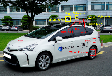
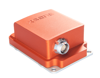
The following results are obtained on the complex urban LiDAR dataset [11], that consists of data recorded on a consumer car moving in complex urban environments, e.g. metropolitan areas, large building complexes and underground parking lots, see Figure 6. Our goal is to show that using an IMU of moderate cost, one manages to obtain surprisingly accurate dead reckoning by using state-of-the-art machine learning techniques to detect relevant assumptions that can be fed into a state-of-the-art Kalman filter. The detector is trained on a series of sequences and tested on another sequences, but all sequences involve the same car and inertial sensors. Generalization to different robot and IMU is not considered herein and is left for future work.

Figure 6: The considered dataset [11] contains data logs of a Xsens MTi-300 (right) recorded at $100\text{\,}\mathrm{H}\mathrm{z}$ along with the ground truth pose.

V-A Implementation Details

We provide in this section the detector and filter setting of the RINS-W system. The detector disposes of four LSTMs, one for each motion profile. Each LSTM consists of 2 layers of 250 hidden units and its hidden state is mapped to a score probability by a 2 layers multi-perceptron network with a ReLU activation function and is followed by a sigmoid function [8] that outputs a scalar value in the range $\left[0,\leavevmode\nobreak\ 1\right]$. We implement the detector on PyTorch and set the threshold values to 0.95 for ($z_{n}^{\mathrm{\textsc{vel}}}$, $z_{n}^{\mathrm{\textsc{ang}}}$), and 0.5 for ($z_{n}^{\mathrm{\textsc{lat}}}$, $z_{n}^{\mathrm{\textsc{up}}}$). The filter operates at the $100\text{\,}\mathrm{H}\mathrm{z}$ IMU rate ($dt=${10}^{-2}\text{\,}\mathrm{s}$$) and its noise covariance matrices are parameterized as

$$\mathbf{Q}_{n} =\operatorname{diag}\left(\sigma_{\bm{\omega}}^{2}\mathbf{I},\leavevmode\nobreak\ \sigma_{\mathbf{a}}^{2}\mathbf{I},\leavevmode\nobreak\ \sigma_{\mathbf{b}_{\bm{\omega}}}^{2}\mathbf{I},\leavevmode\nobreak\ \sigma_{\mathbf{b}_{\mathbf{a}}}^{2}\mathbf{I}\right),$$ (31)

$$\mathbf{N}_{n} =\operatorname{diag}\left(\sigma_{\mathrm{\textsc{vel},\mathbf{v}}}^{2}\mathbf{I},\leavevmode\nobreak\ \sigma_{\mathrm{\textsc{vel},\mathbf{a}}}^{2}\mathbf{I},\leavevmode\nobreak\ \sigma_{\mathrm{\textsc{ang}}}^{2}\mathbf{I},\leavevmode\nobreak\ \sigma_{\mathrm{\textsc{lat}}}^{2},\leavevmode\nobreak\ \sigma_{\mathrm{\textsc{up}}}^{2}\right),$$ (32)

where we set $\sigma_{\bm{\omega}}=$0.01\text{\,}\mathrm{r}\mathrm{a}\mathrm{d}\mathrm{/}\mathrm{s}$$, $\sigma_{\mathbf{a}}=$0.2\text{\,}\mathrm{m}\mathrm{/}\mathrm{s}^{2}$$, $\sigma_{\mathbf{b}_{\bm{\omega}}}=$0.001\text{\,}\mathrm{r}\mathrm{a}\mathrm{d}\mathrm{/}\mathrm{s}$$, $\sigma_{\mathbf{b}_{\mathbf{a}}}=$0.02\text{\,}\mathrm{m}\mathrm{/}\mathrm{s}^{2}$$ for the noise propagation covariance matrix $\mathbf{Q}_{n}$, and $\sigma_{\mathrm{\textsc{vel},\mathbf{v}}}=$1\text{\,}\mathrm{m}\mathrm{/}\mathrm{s}$$, $\sigma_{\mathrm{\textsc{vel},\mathbf{a}}}=$0.4\text{\,}\mathrm{m}\mathrm{/}\mathrm{s}^{2}$$, $\sigma_{\mathrm{\textsc{ang}}}=$0.04\text{\,}\mathrm{r}\mathrm{a}\mathrm{d}\mathrm{/}\mathrm{s}$$, $\sigma_{\mathrm{\textsc{lat}}}=$3\text{\,}\mathrm{m}\mathrm{/}\mathrm{s}$$, and $\sigma_{\mathrm{\textsc{up}}}=$3\text{\,}\mathrm{m}\mathrm{/}\mathrm{s}$$ for the noise measurement covariance matrix $\mathbf{N}_{n}$.

V-B Detector Training

The detector is trained with the sequences urban06 to urban14, that represents $100\text{\,}\mathrm{k}\mathrm{m}$ of training data (sequences urban00 to urban05 does not have acceleration data). For each sequence, we compute ground truth position velocity $\mathbf{v}_{n}^{\mathrm{\textsc{w}}}$ and angular velocity $\bm{\omega}_{n}$ after differentiating the ground pose and applying smoothing. We then compute the ground-truth $\mathbf{z}_{n}$ by applying a small threshold on the ground truth velocities, e.g. we consider $z_{n}^{\mathrm{\textsc{vel}}}=1$ if $\|\mathbf{v}_{n}^{\mathrm{\textsc{w}}}\|<$0.01\text{\,}\mathrm{m}\mathrm{/}\mathrm{s}$$. We set similarly the other motion profiles and use a threshold of $0.005\text{\,}\mathrm{r}\mathrm{a}\mathrm{d}\mathrm{/}\mathrm{s}$ for the angular velocity, and a threshold of $0.1\text{\,}\mathrm{m}\mathrm{/}\mathrm{s}$ for the lateral and upward velocities.

The detector is trained during 500 epochs with the ADAM optimizer [32], whose learning rate is initializing at $10^{-3}$ and managed by a learning rate scheduler. Regularization is enforced with dropout layer, where $p=0.4$ is the probability of any element to be zero. We use the binary cross entropy loss since we have four binary classification problems. For each epoch, we organize data as a batch of $2\text{\,}\mathrm{m}\mathrm{i}\mathrm{n}$ sequences, where we randomly set the start instant of each sequence, and constraints each starting sequence to be a stop of at minimum $1\text{\,}\mathrm{s}$. Training the full detector takes less than one day with a GTX 1080 GPU.

test seq.	wheels odo.	odo. + FoG	RINS-W
15: $16\text{\,}\mathrm{m}\mathrm{i}\mathrm{n}$	$19$ / $5$ / $36$	7 / 2 / 7	$\mathbf{7}$ / $5$ / $12$
16: $73\text{\,}\mathrm{m}\mathrm{i}\mathrm{n}$	$140$ / $127$ / $1166$	$34$ / $20$ / 164	$\mathbf{27}$ / $\mathbf{11}$ / $\mathbf{20}$
17: $19\text{\,}\mathrm{m}\mathrm{i}\mathrm{n}$	$96$ / $64$ / $427$	$58$ / $51$ / $166$	$\mathbf{13}$ / $\mathbf{11}$ / $\mathbf{13}$
15-17:	$114$ / $98$ / $677$	$34$ / $30$ / $152$	$\mathbf{22}$ / $\mathbf{10}$ / $\mathbf{18}$
$108\text{\,}\mathrm{m}\mathrm{i}\mathrm{n}$

Table 1: Results obtained by the 3 methods on urban test sequences 15, 16, 17 in terms of: $m$-ATE /aligned $m$-ATE / final distance error to ground truth, in $\text{\,}\mathrm{m}$. Last line is the concatenation of the three sequences. Direct IMU integration always diverges. The proposed RINS-W outperforms differential wheel speeds based odometry and outperforms on average (see last line) the expensive combination of odometry + FoG. Indeed, RINS-W uses an IMU with gyro stability of $10\text{\,}\deg\mathrm{/}\mathrm{h}$, whereas FoG stability is $0.05\text{\,}\deg\mathrm{/}\mathrm{h}$.

V-C Evaluation Metrics

To assess performances we consider three error metrics:

V-C1 Mean Absolute Trajectory Error ($m$-ATE)

which averages the planar translation error of estimated poses with respect to a ground truth trajectory and is less sensitive to single poor estimates than root mean square error;

V-C2 Mean Absolute Aligned Trajectory Error (aligned $m$-ATE)

that first aligns the estimated trajectory with the ground truth and then computes the mean absolute trajectory error. This metric evaluates the consistency of the trajectory estimates;

V-C3 Final distance error

which is the final distance between the un-aligned estimates and the ground truth.

V-D Trajectory Results

After training the detector on sequences urban06 to urban14, we evaluate the approach on test sequences urban15 to urban17, that represent $40\text{\,}\mathrm{k}\mathrm{m}$ of evaluation data. We compare 4 methods:

• IMU: the direct integration of the IMU measurements based on (1)-(7), that is, pure inertial navigation;

• Odometry: the integration of a differential wheel encoder which computes linear and angular velocities;

• RINS-W (ours): the proposed approach, that uses only the IMU signals and involves no other sensor.

• Odometry + FoG: the integration of a differential wheel encoder which computes only linear velocity. The angular velocity is obtained after integrating the increments of an highly accurate and costly KVH DSP-1760 Fiber optics Gyro (FoG). The FoG gyro bias stability ($0.05\text{\,}\deg\mathrm{/}\mathrm{h}$) is 200 times smaller than the gyro stability of the IMU used by RINS-W;

Fig. 7: Ground truth and trajectory estimates for the test sequence urban15 of the car dataset [11]. RINS-W obtains results comparable with FoG-based odometry.

We delay each sequence such that the trajectory starts with a $1\text{\,}\mathrm{s}$ stop to initialize the orientation and the biases, see Section IV-B. Bias initialization is also performed for IMU pure integration and the FoG. Optimized parameters for wheel speeds sensors calibration are provided by the dataset.

Experimental results in terms of error with respect to ground truth are displayed in Table 1, and illustrated on Figures 1, 7, and 8. Results demonstrate that:

• directly integrating IMU leads to divergence at the first turn, even after a careful calibration procedure;

• wheel-based differential odometry accurately estimates the linear velocity but has troubles estimating the yaw during sharp bends, even if the dataset has been obtained in an urban environment and the odometry parameters are calibrated. This drawback may be remedied at the expense of using an additional high-cost gyroscope;

• the proposed scheme completely outperforms wheel encoders, albeit in urban environment. More surprisingly, our approach competes with the combination of wheel speed sensors + (200 hundred times more accurate) Fyber optics Gyro, and even outperforms it on average.

Furthermore, although comparisons were performed in 2D environments our method yields the full 3D pose of the robot, and as such is compatible with non planar environments.

Fig. 8: Ground truth and trajectory estimates for the test sequence urban17 of the car dataset [11]. RINS-W clearly outperforms the odometry and even the odometry + FoG solution. We note that RINS-W accurately follows the interchange road located at $(x=2,y=1)$.

V-E Discussion

The performances of RINS-W can be explained by: $i$) a false-alarm free detector; $ii$) the fact incorporating side information into IMU integration obviously yields better results; and $iii$) the use of a recent IEKF that has been proved to be well suited for localization tasks.

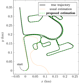
We also emphasize the importance of (11) and (13) in the procedure, i.e. applying (25)-(26). For illustration, we consider sequence urban07 of [11], where the vehicle moves during 7 minutes without stop so that ZUPT may not be used. We implement the detector trained on the first 6 sequences, and compare the proposed RINS-W to a RINS-W which does not use updates (25)-(26) when detected, see Figure 9. Clearly, the reduced RINS-W diverges at the first turn whereas the full RINS-W is accurate along all the trajectory and obtains a final distance w.r.t. ground truth of $5\text{\,}\mathrm{m}$. In contrast, odometry + FoG achieves $16\text{\,}\mathrm{m}$.

Fig. 9: Comparison on the sequence urban07 between proposed RINS-W, and a similar algorithm that does not use zero lateral and vertical velocities assumptions brought by the detector, see (25)-(26). The final distance between ground truth and RINS-W estimates is as small as $5\text{\,}\mathrm{m}$, whereas ignoring (25)-(26) yields divergence.

V-F Detector Evaluation

In Section V-E we mentioned three possible reasons explaining the performances of RINS-W, but could not assess what is owed to each. To assess the detector’s performance, and to demonstrate the interest of our powerful deep neural network based approach (see Section IV-A) we focus on the zero velocity detection (9), and compare the detector with the Acceleration-Moving Variance Detector (AMVD) [20] on the test sequences urban15-17, which represent $64.10^{4}$ measurements. The AMVD computes the accelerometer variance over a sample window $W=10^{2}$ and assumes the vehicle is stationary if the variance falls below a threshold $\gamma=10^{-3}$. To make sure AMVD performs at its best, the parameters $W$ and $\gamma$ are optimized by grid search on the test sequences. Results are shown in Table 2 and demonstrate the detector is more accurate than this “ideal” AMVD.

$z_{n}^{\mathrm{vel}}$ detection	ideal AMVD	our detector
true positive / false pos.	$47.10^{4}$ / $4.10^{3}$	$\mathbf{48.10^{4}}$ / $\mathbf{7.10^{2}}$
true negative / false neg.	$\mathbf{16.10^{4}}$ / $1.10^{4}$	$\mathbf{16.10^{4}}$ / $\mathbf{9.10^{3}}$
precision / recall	$0.974$ / $\mathbf{0.940}$	$\mathbf{0.996}$ / $\mathbf{0.940}$

Table 2: Results on zero velocity (9) detection obtained by an ideal AMVD [20] and the proposed detector on test sequences urban15-17. The proposed detector systematically obtains better results and precision. This is remarkable because the detector is not trained on those sequences, whereas AMVD parameters were optimized on the considered test sequences.

VI Conclusion

This paper proposes a novel approach for robust inertial navigation for wheeled robots (RINS-W). Even if an autonomous vehicle is equipped with wheel encoders, LiDAR, and vision besides the IMU, the algorithm may be run in parallel for safety, in case of sensor failure, or more simply for validation such as slip angle monitoring [1]. Our approach exploits deep neural networks to identify specific patterns in wheeled vehicle motions and incorporates this knowledge in IMU integration for localization. The entire algorithm is fed with IMU signals only, and requires no other sensor. The method leads to surprisingly accurate results, and opens new perspectives for combination of data-driven methods with well established methods for autonomous systems. Moreover, the pseudo measurements output by the detector are not reserved for dead reckoning and may prove useful in any fusion scheme. In future work, we would like to address the learning of the Kalman covariance matrices, and also the issue of generalization from one vehicle to another.

Appendix A

The Lie group $SE_{2}(3)$ is an extension of the Lie group $SE(3)$ and is described as follow, see [9] for more details. A $5\times 5$ matrix $\raisebox{1.0pt}{$\bm{\chi}$}_{n}\in SE_{2}(3)$ is defined as

$$\raisebox{1.0pt}{$\bm{\chi}$}_{n}=\left[\begin{array}[]{ccc}\mathbf{R}_{n}&\mathbf{v}_{n}^{\mathrm{\textsc{w}}}&\mathbf{p}_{n}^{\mathrm{\textsc{w}}}\\ \mathbf{0}&\lx@intercol\hfil\mathbf{I}\hfil\lx@intercol\end{array}\right]\in SE_{2}(3).$$ (35)

The uncertainties $\bm{\xi}_{n}\in\mathbb{R}^{9}$ are mapped to the Lie algebra $\mathfrak{se}_{2}(3)$ through the transformation $\bm{\xi}_{n}\mapsto\bm{\xi}_{n}^{\wedge}$ defined as

$$\bm{\xi}_{n} =\left(\bm{\xi}^{\mathbf{R}}_{n},\leavevmode\nobreak\ \bm{\xi}^{\mathbf{v}}_{n},\leavevmode\nobreak\ \bm{\xi}^{\mathbf{p}}_{n}\right),$$ (36)

$$\bm{\xi}^{\wedge}_{n} =\left[\begin{array}[]{ccc}\left(\bm{\xi}^{\mathbf{R}}_{n}\right)_{\times}&\bm{\xi}^{\mathbf{v}}_{n}&\bm{\xi}^{\mathbf{p}}_{n}\\ \lx@intercol\hfil\mathbf{0}\hfil\lx@intercol\end{array}\right]\in\mathfrak{se}_{2}(3),$$ (39)

where $(\cdot)_{\times}$ transforms a vector to a skew-symmetric matrix, $\bm{\xi}^{\mathbf{R}}_{n}\in\mathbb{R}^{3}$, $\bm{\xi}^{\mathbf{v}}_{n}\in\mathbb{R}^{3}$ and $\bm{\xi}^{\mathbf{p}}_{n}\in\mathbb{R}^{3}$. The closed-form expression for the exponential map is given as

$$\exp_{SE_{2}(3)}\left(\bm{\xi}_{n}\right)=\mathbf{I}+\bm{\xi}_{n}^{\wedge}+a(\bm{\xi}_{n}^{\wedge})^{2}+b(\bm{\xi}_{n}^{\wedge})^{3},$$ (40)

where $a=\frac{1-\cos\left(\|\bm{\xi}^{\mathbf{R}}_{n}\|\right)}{\|\bm{\xi}^{\mathbf{R}}_{n}\|}$ and $b=\frac{\|\bm{\xi}^{\mathbf{R}}_{n}\|-\sin\left(\|\bm{\xi}^{\mathbf{R}}_{n}\|\right)}{\|\bm{\xi}^{\mathbf{R}}_{n}\|^{3}}$.

Appendix B

Following the Right IEKF of [9], the Jacobians required for the computation of the filter propagation (20) are given as

$$\mathbf{F}_{n}=\mathbf{I}+\begin{bmatrix}\mathbf{0}&\mathbf{0}&\mathbf{0}&-\mathbf{R}_{n}&\mathbf{0}\\ (\mathbf{g})_{\times}&\mathbf{0}&\mathbf{0}&-(\mathbf{v}_{n}^{\mathrm{\textsc{w}}})_{\times}\mathbf{R}_{n}&-\mathbf{R}_{n}\\ \mathbf{0}&\mathbf{I}&\mathbf{0}&-(\mathbf{p}_{n}^{\mathrm{\textsc{w}}})_{\times}\mathbf{R}_{n}&\mathbf{0}\\ \mathbf{0}&\mathbf{0}&\mathbf{0}&\mathbf{0}&\mathbf{0}\\ \mathbf{0}&\mathbf{0}&\mathbf{0}&\mathbf{0}&\mathbf{0}\end{bmatrix}dt,$$ (41)

$$\mathbf{G}_{n}=\begin{bmatrix}\mathbf{R}_{n}&\mathbf{0}&\mathbf{0}&\mathbf{0}\\ (\mathbf{v}_{n}^{\mathrm{\textsc{w}}})_{\times}\mathbf{R}_{n}&\mathbf{R}_{n}&\mathbf{0}&\mathbf{0}\\ (\mathbf{p}_{n}^{\mathrm{\textsc{w}}})_{\times}\mathbf{R}_{n}&\mathbf{0}&\mathbf{0}&\mathbf{0}\\ \mathbf{0}&\mathbf{0}&\mathbf{I}&\mathbf{0}\\ \mathbf{0}&\mathbf{0}&\mathbf{0}&\mathbf{I}\end{bmatrix}dt,$$ (42)

when $\hat{z}_{n}^{\mathrm{\textsc{vel}}}=0$ and $\hat{z}_{n}^{\mathrm{\textsc{ang}}}=0$. Otherwise, we set the appropriate rows to zero in $\mathbf{F}_{n}$ and $\mathbf{G}_{n}$, i.e.:

• if $\hat{z}_{n}^{\mathrm{\textsc{vel}}}=1$ we set the 4 to 9 rows of the right part of $\mathbf{F}_{n}$ in (41) and of $\mathbf{G}_{n}$ to zero.

• if $\hat{z}_{n}^{\mathrm{\textsc{ang}}}=1$ we set the 3 first rows of the right part of $\mathbf{F}_{n}$ in (41) and of $\mathbf{G}_{n}$ to zero.

Once again following [9], the measurement Jacobians used in the filter update (27)-(30) are given as

$$\mathbf{H}_{n}^{\mathrm{\textsc{vel}}} =\begin{bmatrix}\mathbf{0}&\mathbf{R}_{n}^{T}&\mathbf{0}&\mathbf{0}&\mathbf{0}\\ \mathbf{R}_{n}^{T}(\mathbf{g})_{\times}&\mathbf{0}&\mathbf{0}&\mathbf{0}&-\mathbf{I}\end{bmatrix},$$ (43)

$$\mathbf{H}_{n}^{\mathrm{\textsc{ang}}} =\begin{bmatrix}\mathbf{0}&\mathbf{0}&\mathbf{0}&-\mathbf{I}&\mathbf{0}\end{bmatrix},$$ (44)

and we obtains $\mathbf{H}_{n}^{\mathrm{\textsc{lat}}}$ and $\mathbf{H}_{n}^{\mathrm{\textsc{up}}}$ as respectively the second and third row of $\mathbf{H}_{n}^{\mathrm{\textsc{vel}}}$.

References

- [1] OxTS. (2018) Why it is Necessary to Integrate an Inertial Measurement Unit with Imaging Systems on an Autonomous Vehicle. [Online]. Available: https://www.oxts.com/technical-notes/why-use-ins-with-autonomous-vehicle/
- [2] J. Collin, P. Davidson, M. Kirkko-Jaakkola, and H. Leppäkoski, “Inertial Sensors and Their Applications,” in Handbook of Signal Processing Systems. Springer, 2018, pp. 69–96.
- [3] M. Kok, J. Hol, and T. Schön, “Using Inertial Sensors for Position and Orientation Estimation,” Foundations and Trends® in Signal Processing, vol. 11, no. 1-2, pp. 1–153, 2017.
- [4] Safran. (2018) Inertial navigation systems. [Online]. Available: https://www.safran-group.com/fr/video/13612
- [5] C. Cadena, L. Carlone, H. Carrillo, Y. Latif, D. Scaramuzza, J. Neira, I. Reid, and J. Leonard, “Past, Present, and Future of Simultaneous Localization and Mapping: Toward the Robust-Perception Age,” IEEE T-RO, pp. 1309–1332, 2016.
- [6] K. Sun, K. Mohta, B. Pfrommer, M. Watterson, S. Liu, Y. Mulgaonkar, C. J. Taylor, and V. Kumar, “Robust Stereo Visual Inertial Odometry for Fast Autonomous Flight,” IEEE RA-L, vol. 3, no. 2, pp. 965–972, 2018.
- [7] J.-E. Deschaud, “IMLS-SLAM: Scan-to-Model Matching Based on 3D Data,” in IEEE ICRA, 2018.
- [8] I. Goodfellow, Y. Bengio, and A. Courville, Deep Learning. The MIT press, 2016.
- [9] A. Barrau and S. Bonnabel, “The Invariant Extended Kalman Filter as a Stable Observer,” IEEE Trans. on Automatic Control, vol. 62, no. 4, pp. 1797–1812, 2017.
- [10] ——, “Invariant Kalman Filtering,” Annual Review of Control, Robotics, and Autonomous Systems, vol. 1, no. 1, pp. 237–257, 2018. [Online]. Available: https://doi.org/10.1146/annurev-control-060117-105010
- [11] J. Jeong, Y. Cho, Y.-S. Shin, H. Roh, and A. Kim, “Complex Urban LiDAR Data Set,” in IEEE ICRA, 2018.
- [12] A. Barrau and S. Bonnabel, “Aligment Method for an Inertial Unit,” patent 15/037,653, 2016.
- [13] K. Wu, T. Zhang, D. Su, S. Huang, and G. Dissanayake, “An invariant-EKF VINS algorithm for improving consistency,” in IEEE IROS, 2017, pp. 1578–1585.
- [14] S. Heo and C. G. Park, “Consistent EKF-Based Visual-Inertial Odometry on Matrix Lie Group,” IEEE Sensors Journal, vol. 18, no. 9, pp. 3780–3788, 2018.
- [15] M. Brossard, S. Bonnabel, and A. Barrau, “Unscented Kalman Filter on Lie Groups for Visual Inertial Odometry,” in IEEE IROS, 2018.
- [16] R. Hartley, M. G. Jadidi, J. W. Grizzle, and R. M. Eustice, “Contact-Aided Invariant Extended Kalman Filtering for Legged Robot State Estimation,” in Robotics Science and Systems, 2018.
- [17] K. Wu, C. Guo, G. Georgiou, and S. Roumeliotis, “VINS on Wheels,” in IEEE ICRA, 2017, pp. 5155–5162.
- [18] F. Zheng, H. Tang, and Y.-H. Liu, “Odometry Vision Based Ground Vehicle Motion Estimation With SE(2)-Constrained SE(3) Poses,” IEEE Trans. on Cybernetics, pp. 1–12, 2018.
- [19] A. Ramanandan, A. Chen, and J. Farrell, “Inertial Navigation Aiding by Stationary Upyears,” IEEE Trans. on Intelligent Transportation Systems, vol. 13, no. 1, pp. 235–248, 2012.
- [20] I. Skog, P. Handel, J. O. Nilsson, and J. Rantakokko, “Zero-Velocity Detection—An Algorithm Evaluation,” IEEE Trans. on Biomedical Engineering, vol. 57, no. 11, pp. 2657–2666, 2010.
- [21] G. Dissanayake, S. Sukkarieh, E. Nebot, and H. Durrant-Whyte, “The Aiding of a Low-cost Strapdown Inertial Measurement Unit Using Vehicle Model Constraints for Land Vehicle Applications,” IEEE T-ROA, vol. 17, no. 5, pp. 731–747, 2001.
- [22] A. Solin, S. Cortes, E. Rahtu, and J. Kannala, “Inertial Odometry on Handheld Smartphones,” in FUSION, 2018.
- [23] D. Atchuthan, A. Santamaria-Navarro, N. Mansard, O. Stasse, and J. Solà, “Odometry Based on Auto-Calibrating Inertial Measurement Unit Attached to the Feet,” in ECC, 2018.
- [24] H. Yan, Q. Shan, and Y. Furukawa, “RIDI: Robust IMU Double Integration,” in ECCV, 2018.
- [25] B. Wagstaff and J. Kelly, “LSTM-Based Zero-Velocity Detection for Robust Inertial Navigation,” in IPIN, 2018.
- [26] S. Cortes, A. Solin, and J. Kannala, “Deep Learning Based Speed Estimation for Constraining Strapdown Inertial Navigation on Smartphones,” IEEE MLSP workshop, 2018.
- [27] C. Chen, X. Lu, A. Markham, and N. Trigoni, “IONet: Learning to Cure the Curse of Drift in Inertial Odometry,” in AAAI, 2018.
- [28] C. Chen, P. Zhao, C. X. Lu, W. Wang, A. Markham, and N. Trigoni, “OxIOD: The Dataset for Deep Inertial Odometry,” 2018.
- [29] M. Brossard and S. Bonnabel, “Learning Wheel Odometry and IMU Errors for Localization,” in IEEE ICRA, 2019.
- [30] T. Haarnoja, A. Ajay, S. Levine, and P. Abbeel, “Backprop KF: Learning Discriminative Deterministic State Estimators,” in NIPS, 2016.
- [31] T. Barfoot and P. Furgale, “Associating Uncertainty With Three-Dimensional Poses for Use in Estimation Problems,” IEEE T-RO, vol. 30, no. 3, pp. 679–693, 2014.
- [32] D. P. Kingma and J. Ba, “Adam: A Method for Stochastic Optimization,” in ICLR, 2014.