Accelerating Training of Deep Neural Networks with a Standardization Loss

Abstract

A significant advance in accelerating neural network training has been the development of normalization methods (Ioffe & Szegedy, 2015; Wu & He, 2018; Ba et al., 2016; Salimans & Kingma, 2016), permitting the training of deep models both faster and with better accuracy. These advances come with practical challenges: for instance, batch normalization ties the prediction of individual examples with other examples within a batch, resulting in a network that is heavily dependent on batch size. Layer normalization and group normalization are data-dependent and thus must be continually used, even at test-time. To address the issues that arise from using explicit normalization techniques, we propose to replace existing normalization methods with a simple, secondary objective loss that we term a standardization loss. This formulation is flexible and robust across different batch sizes and surprisingly, this secondary objective accelerates learning on the primary training objective. Because it is a training loss, it is simply removed at test-time, and no further effort is needed to maintain normalized activations. We find that a standardization loss accelerates training on both small- and large-scale image classification experiments, works with a variety of architectures, and is largely robust to training across different batch sizes.

1 Introduction

Recent progress in machine learning has been fueled by the recognition that a key ingredient of state-of-the-art systems is building larger models on increasingly larger datasets (Halevy et al., 2009). Deep learning (LeCun et al., 2015; Goodfellow et al., 2016) has been one such direction where models provide increasing gains in predictive performance as model size and datasets grow (e.g. (Williams et al., 2015)). The limiting factor in building deep learning models is thus the speed at which one may train such systems on large amounts of data. This limitation has yielded new classes of specialized hardware (Jouppi et al., 2018; Chetlur et al., 2014) as well as driven the development of new model architectures (Ioffe, 2017; Wu & He, 2018; Hochreiter & Schmidhuber, 1997) and optimization methods (Duchi et al., 2011; Tieleman & Hinton, 2012; Kingma & Ba, 2015) – all with the goal of accelerating neural network training.

Batch normalization (BN) (Ioffe & Szegedy, 2015) is one method for accelerating neural network training that has become a necessary and standard component in many state-of-the-art systems in image classification (Szegedy et al., 2016b, a; He et al., 2016a, b), object detection (Huang et al., 2017), image segmentation (Chen et al., 2018; Zhao et al., 2017), generative models (Radford et al., 2015; Karras et al., 2017) and other problems (Cooijmans et al., 2016). BN explicitly requires a network to maintain normalized (i.e. standardized) activations. The resulting network benefits from accelerated learning by up to an order-of-magnitude (Ioffe & Szegedy, 2015), and makes some networks trainable that were previously untrainable (e.g. Radford et al. (2015)).

In spite of its successes, BN does offer some serious challenges and limitations: (1) BN is poorly understood and there is no general consensus on how it works (Santurkar et al., 2018; Bjorck et al., 2018; Kohler et al., 2018) making a successful application of BN to some architectures challenging (Ba et al., 2016; Laurent et al., 2016; Cooijmans et al., 2016), (2) BN complicates training significantly because it couples individual training examples and makes training on small batch sizes or non i.i.d. statistics difficult (but see (Ioffe, 2017)), (3) BN does not permit a unified training objective because some parameters (i.e. moments used for inference) are estimated with moving averages independent of the training objective.

Alternative forms of normalization have since been proposed that act on different dimensions of the network activations. Layer normalization (Ba et al., 2016) and group normalization (Wu & He, 2018) both reduce the dependency of normalized models on batch dimension, but introduce the drawback that they require continued use at test-time. Because BN uses separately estimated normalization statistics at inference, these parameters may be ’folded in’ to the previous layer’s weights, ensuring that no extra operations are spent on normalization during inference. Layer and group normalization are data-dependent, and thus must be continually used at test-time.

In this work, we propose a simple method for accelerating neural network training that achieves some of the gains of existing explicit normalization techniques without the need to re-tune hyperparameters. Instead of imposing normalization as a requirement in a network’s structure, we follow a strategy of expressing normalization as an objective loss. This leads to a flexible form of normalization that is robust across different batch sizes for stochastic gradient descent (SGD) and simplifies behavior during inference. Surprisingly, even though the network is now required to minimize a secondary loss, we find that the resulting network trains faster on the original task. Because our approach only involves a loss (rather than making an architectural change), inference-time merely requires removing the loss – as is naturally done after training any machine learning system. In particular, we provide the following contributions in this work:

1. Introduce a secondary objective to penalize activation patterns that diverge from standardized Gaussian distributions.

2. Demonstrate that applying this loss in a small multi-layer perceptron (MLP) and convolutional neural network (CNN) accelerates early training and is somewhat robust to a single added hyperparameter.

3. Demonstrate that such a loss accelerates training up to 2.8 x on large-scale MLPs and a wide range of CNN architectures trained on ImageNet.

4. Show that training with a standardization loss instead of BN results in networks largely insensitive to batch size and provides competitive performance with existing methods.

The outline of this paper is to first discuss the many related techniques in the literature and then introduce the proposed objective to promote standardization. In the following sections, we describe early experiments on a small dataset (MNIST) and demonstrate the relative benefit of this method for accelerating training. Next, we present several results on large-scale classification tasks on image classification (Deng et al., 2009) and 3-D point cloud classification (Wu et al., 2015), highlighting how training speed with the standardization loss is accelerated across a wide variety of architectures. Finally, we show that networks trained with the standardization loss are largely insensitive to batch size.

2 Related Work

2.1 Normalization for accelerating deep learning training

Whitening transformations have long been used as a standard method for preprocessing data to accelerate statistical estimation and learning (Murphy, 2013). Whitening, however, can be computationally challenging for high-dimensional distributions because it requires calculating and inverting a large covariance matrix. These problems are further exacerbated in deep learning systems in which multiple representations are learned simultaneously in an online fashion. These dual challenges make whitening largely intractable in deep learning systems (but see Huang et al. (2018)) and instead has lead to the development of weaker forms of imposing normalization during training.

BN (Ioffe & Szegedy, 2015) is a state-of-the-art solution which explicitly requires that activations in a given layer $\mathbf{x}$ must be standardized (i.e. skipping decorrelation). BN constructs the network representation to be self-normalized across the batch and spatial dimensions in a CNN, and only the batch dimension for an MLP. While BN can greatly accelerate training, it is widely known that this performance boost is predicated on the ability to train with sufficiently large batch size. For smaller batch sizes, the performance gain due to BN drops.

To alleviate issues with small batch sizes, batch renormalization (Ioffe, 2017) introduced two parameters to constrain the first two moments of the distribution. Although this technique was developed to mitigate issues with small batch size, models with batch renormalization still suffer from a decrease in accuracy when trained on very small batch size and still make training dependent on the individual items within a batch.

Another approach that was recently proposed for image models is group normalization (GN) (Wu & He, 2018). GN is a normalization technique specialized for CNNs that divides a given layer into artificial groups, across which the mean and variance are respectively normalized. The resulting models are largely insensitive to batch size but perform below BN in a large batch setting (Wu & He, 2018). Additionally, GN makes no claim about accelerating the speed of training but rather focuses on asymptotic performance.

Finally, other approaches have focused on encouraging normalization during training by improving weight initialization (Kingma & Dhariwal, 2018) or employing a factorized representation such that most network parameters are L2-normalized (Salimans & Kingma, 2016) (see also (Arpit et al., 2016)).

2.2 Auxiliary losses to shape the distribution of activations

Instead of building an architecture to constrain that a given layer’s activations are standardized, we instead focus on constructing an auxiliary loss to shape the distribution of the activations. Applying a loss to shape the distribution of activations has been explored in the context of autoencoders to sparsify a given layer’s representation (Lee et al., 2008; Nair & Hinton, 2009; Gao & Zhou, 2016; Ngiam et al., 2011). Specifically, in order to encourage sparsity, the discretized activations of a given layer were penalized with respect to their distance from a Bernoulli distribution.

Similarly, Goroshin & LeCun (2013) added an auxiliary objective to networks in order to encourage the representation to be close to the saturating regime of a network’s nonlinearities. The goal of this secondary objective was to improve generalization and provide a defense against adversarial attacks (Gu & Rigazio, 2014).

3 Methods

The following methods focus on training MLPs and CNNs (LeCun et al., 1998), but these methods may be extended to other network architectures (Goodfellow et al., 2016). Let $\mathbf{x}$ be the activation pattern in a given layer of a network, before the nonlinearity is applied. For instance, for a CNN, $\mathbf{x}$ may be a tensor with dimensions $[b,h,w,n]$ corresponding to batch, height, width and channels. For an MLP, $\mathbf{x}$ may be a tensor with dimensions $[b,n]$ corresponding to $n$ neurons.

We consider each $\mathbf{x}$ to be a sample from a $n$-dimensional distribution $P(\mathbf{x})$. We assume that each example in a batch corresponds to a sample from $P(\mathbf{x})$ (Ioffe & Szegedy, 2015). Additionally, in the case of a CNN, we assume ergodicity such that samples across spatial dimensions also represent independent samples from $P(\mathbf{x})$. Hence, in the case of a CNN, we can define $P(\mathbf{x})$ to be an $n$-dimensional distribution across channels in which the maximum likelihood estimate of the mean and variance are the averages across space and batch dimensions.

In the case of BN, one constructs the architecture to impose standardization on the first two moments of $P(\mathbf{x})$. We propose to replace the explicit normalization with a regularization loss that mimics the invariances offered by BN. Consider the KL-divergence of $P(\mathbf{x})$ with respect to a target distribution $Q(\mathbf{x})$:

$$D_{\scriptscriptstyle KL}\big{(}P(\mathbf{x})\;||\;Q(\mathbf{x})\big{)}=\int P(\mathbf{x})\log\frac{P(\mathbf{x})}{Q(\mathbf{x})}d\mathbf{x}$$ (1)

We define the standardization loss as the KL-divergence of $P(\mathbf{x})$ with respect to a standardized Gaussian distribution $\mathcal{N}(\mathbf{x};\mathbf{0},\mathbf{I})$. The standardization loss measures how far a given distribution is from a standardized representation. The loss is calculated at each layer, and the total loss is the sum across all layers. We apply this loss during training by adding it to the primary objective (e.g. cross-entropy loss) with a selected weight.

We make a simplifying assumption that $P(\mathbf{x})$ is Gaussian distributed corresponding to a maximum entropy distribution constrained by the first two moments. The integral for the loss may then be analytically derived (Kingma & Welling (2015) provide a short derivation):

$$D_{\scriptscriptstyle KL}\big{(}P(\mathbf{x})\;||\;\mathcal{N}(\mathbf{x};\mathbf{0},\mathbf{I})\big{)}=\frac{1}{2}\sum^{n}_{i=1}(\mu_{i}^{2}+\sigma_{i}^{2}-\log(\sigma_{i}^{2})-1)$$ (2)

where $\mu_{i}$ and $\sigma_{i}^{2}$ are the mean and variance of dimension $i$ measured from $P(\mathbf{x})$. These statistics are calculated the same way they are calculated in BN, by marginalizing across the spatial and batch dimensions of $\mathbf{x}$ for a CNN or just the batch dimensions of an MLP.

4 Results

4.1 Standardization loss accelerates training on MNIST

Figure 1: Standardization loss accelerates convergence for 3-layer CNN trained on MNIST. (top) Cross entropy loss and (bottom) accuracy across 1000 gradient steps at a low learning rate in a baseline model without normalization (black), standardization loss (red), and batch normalization network (blue) for training (circles) and validation (squares) data. Error bars represent standard deviation across 10 runs.

Figure 2: Regularization and robustness of standardization loss in a 3-layer CNN. (top) Cross entropy loss vs accuracy for MNIST. Note that the baseline network must be trained for 5000 steps in order to achieve comparable accuracies. (bottom) Accuracy after 1000 gradient steps across varying weight on standardization loss. Colors and marks follow Figure 1.

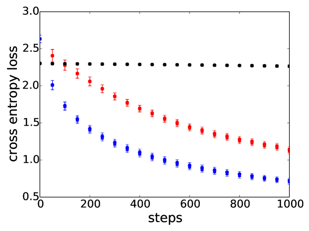
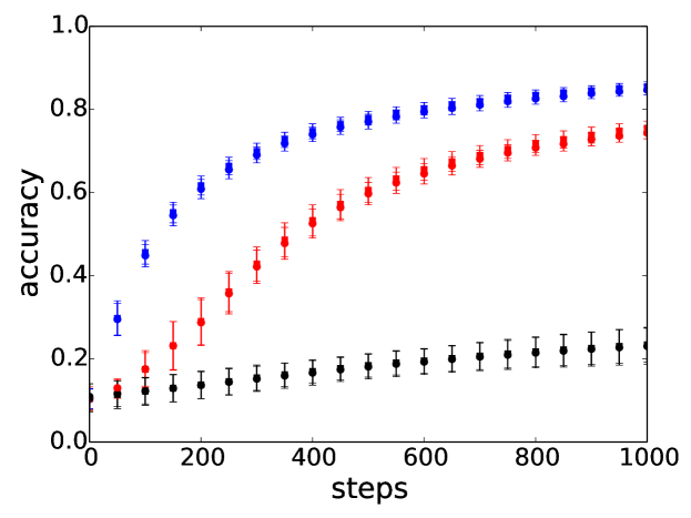
We first examined the standardization loss in a small-scale experimental setting. Specifically, we asked how the simple application of a standardization loss fares as a drop-in replacement for BN. The goal of these experiments is to measure the predictive performance that different normalization configurations attain given a limited and constrained training budget (1000 SGD training steps at a low learning rate of 1e-3).

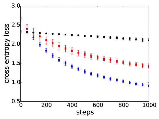
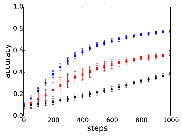
We constructed a small 3-layer CNN (see Appendix for details) and report the mean and standard deviation of the cross entropy loss and cross-validated accuracy across 10 training runs (Figure 1). With BN, the CNN architecture achieves a reasonable accuracy (85.6% $\pm$ $1.1\%$) with a small budget. As expected, removing BN from this network drastically reduced predictive performance (24.6% $\pm$ 6.5%) given an identical, limited training regiment. However, applying an additional standardization loss (weight $=1.0$) to the activations resulted in a performance of 75.2% $\pm$ 2.6%, restoring most of the performance drop due to removing BN.

Across the 1000 training steps, we observed that the application of a standardization loss reliably accelerated training on the primary classification objective for both training and evaluation data, compared to the baseline model without normalization. (Figure 1, top, red vs black). In addition, the application of the standardization loss accelerated arriving at higher predictive accuracies (bottom, red vs black). Note that in all cases the standardization loss did not accelerate training as fast as BN (blue).

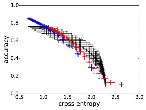
We next asked whether the gain in performance from adding the standardization loss was due to a regularization effect. For example, weight decay is known to improve cross-validated accuracy but does not necessarily accelerate the convergence (Goodfellow et al., 2016; Murphy, 2013). Figure 2 (top) measures the cross entropy loss vs the accuracy for the baseline model (black), BN (blue) and standardization loss (red). If the standardization loss acted as a regularizer that improves the cross-validated accuracy, then the red points would be shifted upward indicating better predictive performance given the same cross entropy value. We do observe a slight upward shift with respect to BN but not the baseline model. We take these results to indicate that most of the gains of the standardization loss over the baseline is instead due to accelerated training.

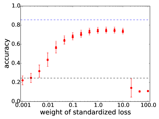
When using the standardization loss, the total loss becomes a combination of the standardization loss and the primary objective. To explore how sensitive the model is to the weight attached to the standardization loss, we systematically varied the strength of the loss and measured the performance of the model after 1000 training steps with the same, limited training budget (Figure 2, bottom). We found that increasing the standardization loss over four orders of magnitude [0.001, 10.0] increased the cross-validated performance – although beyond a particular weighting the predictive performance collapsed.

To explore the generality of our approach, we also examined how well a standardization loss could improve the training performance in a small-scale MLP. We constructed a 3-layer MLP and trained the model on MNIST using the same limited training budget as in the CNN experiments. Figure 3 demonstrates that the application of standardization loss accelerates training both in terms of achieving a lower primary objective (cross entropy) and an improved cross-validated accuracy (red vs black) even though the architectures are identical. Parallel to the CNN version, we do find that although a standardization loss accelerates training, it does not accelerate training as fast as BN (blue). Overall, we took these results on a toy example as a positive signal that the simple application of a secondary standardization loss may accelerate the training on the primary objective of a network .

Figure 3: Standardization loss accelerates convergence for 3-layer MLP trained on MNIST. Panels and colors follow Figure 1.

Figure 4: Evolution of CNN feature distributions for no normalization, standardization loss, and batch normalization trained on MNIST. Black, blue, green and red curves measure the 1, 20, 80, and 99 percentile of the cumulative distributions for the final convolutional layer across training steps. Note the different scale of the y-axis for the no normalization plot.

4.2 Standardization loss results in a similar evolution of feature distributions

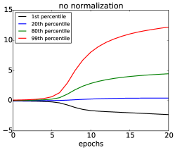
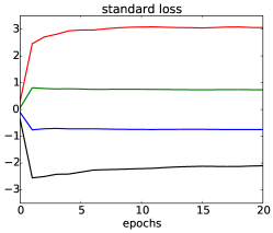
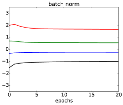
Maintaining stability in the distribution of network features has been a motivating factor for introducing normalization into network architectures (Ioffe & Szegedy, 2015) (but see (Santurkar et al., 2018; Bjorck et al., 2018; Kohler et al., 2018)). We next examine how the feature distributions of a layer evolve across training steps using the 3-layer CNN from our previous experiments. We train the network for 20 epochs (roughly 8.6K steps) and track the distribution of the final layer’s activation across training steps (Figure 4).

Consistent with previous observations (Ioffe & Szegedy, 2015; Wu & He, 2018), removing normalization from the network leads to activation distributions that change notably in shape and scale over the course of training (Figure 4, left). Applying normalization either through BN or a standardization loss restores control over the evolution of the feature distributions (Figure 4, middle and right). Importantly, although the network with the standardization loss is identical in architecture to the baseline network, we see that the simple application of a standardization loss results in a stable distribution that evolves in a way qualitatively similar to a technique which explicitly enforces normalization.

4.3 Standardization loss accelerates training of large-scale MLPs

	# steps	speed-up
baseline	26.6K	-
batch norm	6.1K	4.4 x
standard loss	12.1K	2.2 x

Figure 5: Standardization loss accelerates large-batch training in an MLP on ModelNet40. Speed-ups in table reflect number of steps to reach the maximum accuracy (86.5%) achieved by the baseline model without normalization. See text for details.

After observing positive results for MLPs trained with standardization loss on MNIST, we next moved on to a large-scale task for MLP networks. Classification of point cloud data remains a challenging learning task with applications to robotics and self-driving cars. One common benchmark for assessing performance on point cloud data is ModelNet-40 (Wu et al., 2015) – a classification dataset consisting of 12,311 CAD models across 40 man-made categories. Most state-of-the-art methods on point cloud data employ an MLP with BN as a central component of the architecture (Qi et al., 2017a, b).

We focus on PointNet (Qi et al., 2017a) as a large-scale test of a standardization loss. Our implementation of PointNet with BN achieves 89.3% accuracy, compared to a published value of 89.2%. We also remove BN from PointNet to measure the performance of a no normalization baseline, and find the resulting model achieves an accuracy of 86.5%.

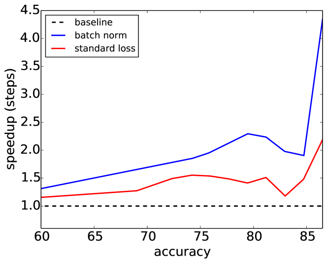
We measured the acceleration of the normalization models over the baseline by calculating the ratio of the number of training steps required to achieve a given accuracy, for the baseline model compared to the normalization model. For instance, the baseline model requires 26.6K training steps to achieve its maximum accuracy (86.5%). The equivalent model with BN only requires 6.1K steps to achieve this same accuracy. Hence, we measure a speed-up due to BN of 4.4 x ($=26.6/6.1$). Figure 5 (blue) plots this speed-up across the entire course of training for BN indicating that BN is consistently faster than no normalization.

We next add a standardization loss to the baseline model, using an identical training scheme (Figure 5, red). The resulting model achieves a 2.2 x speed-up and likewise demonstrates accelerated accuracies over the baseline model across the entire training session. Again we see that a simple secondary objective can achieve some of the gains of BN on a real world task without any of the complications.

4.4 Standardization loss accelerates training of large-scale CNNs

Figure 6: Acceleration of ImageNet top-1 validation accuracy on Inception-v2 over a baseline network by the application of a standardization loss (red) or batch normalization (blue). See Table 1 for summary.

Inception-v2	# steps	speed-up
baseline	1972K	-
batch norm	534K	3.7 x
standard loss	700K	2.8 x

ResNet-50	# steps	speed-up
baseline	89.4K	-
batch norm	39.5K	2.3 x
standard loss	40.0K	2.2 x

Table 1: Acceleration of ImageNet training on Inception-v2 and ResNet-50. Comparison of baseline model with batch normalization and standardization loss. All speed-ups measured in terms of the number of steps to reach the maximum accuracy achieved by the baseline model (69.5% and 70% accuracy, respectively). See text for details.

Given consistent results for both small- and large-scale MLPs, we next asked if there was an analogous result for CNNs. We explored this question in the context of the ImageNet dataset (Deng et al., 2009), across three large-scale CNN architectures: Inception-v2 (Szegedy et al., 2016b), ResNet-50 (He et al., 2016a), and MobileNet-v1 (Howard et al., 2017).

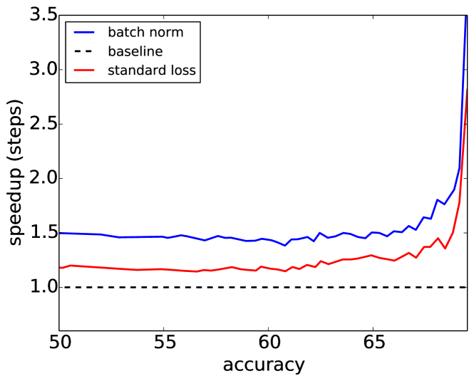
We examined the ResNet-50 and Inception-v2 architectures in order to measure the speed-ups due to normalization. As with PointNet, both CNNs employ BN as a default and thus their hyperparameters are tuned to the use of BN. We found that in order to stabilize Inception-v2 for the baseline setting, it was necessary to lower the learning rate; thus, all comparisons for Inception-v2 are made at this low learning rate (see Appendix for details). Figure 6 measures the speed-up gains over a baseline network by applying the standardization loss (red) and using BN (blue) over the course of training. The standardization loss achieves speed-ups comparable to BN of 2.8 x vs 3.7 x (Table 1, top).

To further explore the generality of the results, we also measure the acceleration of ResNet-50 trained on ImageNet. The baseline model proved more robust to a lack of normalization and did not require adjusting the default learning rate. In line with Inception-v2, we find that the application of a standardization loss accelerates training comparable to BN, with speed-ups of 2.2 x vs 2.3 x (Table 1, bottom).

4.5 Models trained with a standardization loss are robust across batch sizes

BN is known to suffer in performance when trained with very small batch sizes. This issue is known to arise due to the rigid requirement that every batch must be normalized – even when the moments of a distribution are poorly estimated as is the case in a small batch size. In contrast, a standardization loss merely promotes normalization and thus may be more resilient to poorly estimated moments in individual batches. This intuition motivates us to test if indeed a standardization loss may be more robust to choice of batch size and alleviate this major drawback of BN.

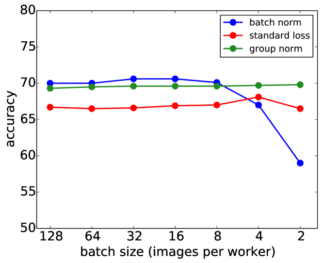
We consider the MobileNet-v1 architecture as this architecture is often employed in domains where batch size is restrictive. Similar to the previous networks we explored, MobileNet-v1 has BN built-in to its architecture. Interestingly, we found that removing BN from MobileNet-v1 destroyed the ability of the network to train above chance rate, even after tuning across a broad range of reasonable hyperparameters. Conversely, by the simple application of the standardization loss (with identical training hyperparameters), MobileNet-v1’s predictive accuracy was largely restored (70.6% vs 66.6% top-1 accuracy at batch size 32).

To investigate the effect of small batch size, we trained MobileNet-v1 ranging in batch sizes from 2 to 128, adopting a linear scaling rule for adjusting the learning rate (Goyal et al., 2019). We compared the performance of BN to the standardization loss across batch size (Figure 7, blue vs red). As previously reported, the performance of BN varies notably across different batch sizes – with small batch sizes typically leading to worse performance. In contrast, a network trained with a standardization loss achieves roughly constant performance (66.5% - 66.9%) across the wide range of batch sizes and demonstrates no precipitous drop in performance at small batch sizes as observed with BN. For batch sizes 2 and 4, the standardization loss outperforms BN.

As previously mentioned, other techniques have recently been introduced to specifically address the issue of the poor small batch performance of BN. Batch renormalization (Ioffe, 2017) mitigates this variability to a degree, but still exhibits some batch dependencies. Group normalization (GN) (Wu & He, 2018) offers a method for calculating normalization statistics that are not dependent on the batch dimension, and achieves state-of-the-art performance for CNNs trained with small batch sizes. As GN represents the state-of-the-art in small batch training of image models, we additionally chose to compare the performance of the standardization loss against GN in MobileNet-v1 training across a large range of batch sizes . Figure 7 (green) highlights that GN indeed exhibits robustness to batch size and outperforms the standardization loss. Note that GN employs a distinct and complimentary form of normalization that is specific to CNNs and there are trade-offs in using these techniques that are addressed in the Discussion. Nonetheless, the application of a standardization loss does provide a simple method for accelerating training that is largely invariant to batch size.

Figure 7: Top-1 validation accuracy of batch normalization, group normalization, and standardization loss networks trained with different batch sizes.

5 Discussion

In this work we have introduced a simple auxiliary loss that encourages the distribution of activations in a deep network towards a standardized Gaussian. We find that adding this secondary objective accelerates the training by almost 2-fold on the primary classification objective for a range of network architectures, and the resulting network can be trained across a wide range of batch sizes.

The gain of our method over other normalization techniques is simplicity and wide applicability to several architectures and problems. Existing normalization techniques are highly specialized and only apply to certain neural network architectures and training setups. BN performs poorly when the activation moments are poorly estimated (e.g. small batch size, non-i.i.d. batches). Additionally, BN requires the user to maintain moving averages at test-time which makes it difficult to apply to certain architectures (e.g. recurrent neural networks). GN addresses the small batch size problem of BN, but it is only applicable to convolutional models, and therefore another technique must be used for training MLPs and recurrent networks with small or non-i.i.d.. batches (e.g. layer normalization, LN). LN empirically works well for MLPs but often does not perform as well as BN for CNNs (Ba et al., 2016). Further, techniques like GN and LN require continued normalization at test-time, demanding an extra pass over the activations at each layer of the network for each prediction step. This may be prohibitive for memory-constrained devices (e.g. mobile and edge devices) and may slow down inference notably. Weight normalization is a simple and architecture-invariant approach that is very successful for small-scale problems, but does not seem to scale well to large-scale problems (Gitman & Ginsburg, 2017). In the experimental settings we considered, our approach to normalization is (1) robust to batch size, (2) applies to both MLPs and CNNs, (3) does not require explicit inference-time normalization, and (4) works in both small- and large-scale settings.

While we find that our method is successful in accelerating training and asymptotic accuracy over networks without normalization, we see lower asymptotic accuracies compared to BN. We note that we did not re-tune hyperparameters for models built with BN as a default, and it is likely that re-tuning could give an accuracy boost. Another possible explanation for the performance difference is that explicit normalization techniques ensure standardized activations from the very first training step, whereas training with a standardization loss requires multiple steps of SGD before the loss decreases and the activations are sufficiently standardized. Better understanding of the differences between a loss-based approach to normalization and existing explicit normalization techniques may allow for networks to benefit even more from a standardization loss.

This work opens up several interesting avenues for further exploration of the application of a standardization loss. Recurrent networks present a challenging domain in which standard normalization techniques do not work well, and specialized variants are required (Ba et al., 2016; Laurent et al., 2016; Cooijmans et al., 2016). Because a standardization loss provides a less stringent form of normalization, it would be interesting to explore the degree to which this method generalizes to these forms of architectures. Likewise, the application of a standardization loss may be particularly advantageous in a stochastic training setting in which the data is not i.i.d. (e.g. metric learning, continual learning) and enforcing that a given batch should be strictly normalized is overly restrictive. Commonly used normalization methods are impeded because the batch statistics provide a skewed perspective of the dataset statistics, which in turn limits training performance (but see (Ioffe, 2017)).

This work focused on encouraging the activations of a given layer towards a standardized Gaussian distribution. Another interesting direction is to apply the same standardization loss but encourage other types of distributional forms. For instance, a simple extension is to require that the activations at a given layer are not just standardized but decorrelated as well. Although more computationally demanding, such a requirement may lead to accuracy improvements (Huang et al., 2018). Another direction to consider is sparsity. Sparsity is well known to improve generalization, and replacing the target distribution with a Laplace or Bernoulli distribution may yield benefits in representational ability, particularly in the context of unsupervised learning (Lee et al., 2008; Nair & Hinton, 2009; Gao & Zhou, 2016; Ngiam et al., 2011).

Appendix A Details of model training

A.1 CNN MNIST

We trained a small 3-layer CNN with 32, 16 and 8 filters ($5\times 5$, stride 2) in each layer and ReLU nonlinearities. The network was trained with SGD at a learning rate of 1e-3 and a batch size of 128. We trained the model for 1000 gradient updates, which corresponds to training with 2.13 epochs of the training set. All models used a weight decay of 4e-5 and the network trained with standardization loss used a weight of 1.0. The BN network used an additive shift parameter after the normalization at each layer (no scale parameter was necessary due to the use of the ReLU nonlinearity).

A.2 MLP MNIST

The MLP we trained had 3-layers with 100 units per layer and used ReLU nonlinearities. We used an identical training scheme to the CNN training. That is, we trained for 1000 SGD steps with a batch size of 128, learning rate of 1e-3 and weight decay of 4e-5. The standardization loss was weighted by 1.0, and the BN network had shift parameters at each layer.

A.3 PointNet (Qi et al., 2017a)

We trained a PointNet with no normalization, standardization loss, and BN each on a single GPU. For all experiments PointNet was optimized using the ADAM optimizer with momentum of 0.9, and a starting learning rate of 1e-3 that was decayed by half every 20 epochs. We used a batch size of 32 and ReLU nonlinearities. The BN network applied a scale and shift at each layer. We also found that the standardization loss network benefited from such scale and shift parameters. The standardization loss is weighted 1e-3.

A.4 Inception-v2 (Szegedy et al., 2016b)

We trained Inception-v2 on 8 Tensor Processing Unit (TPU) cores at a batch size of 128 images per core (1024 total). We used the RMSProp optimizer with a base learning rate of 0.006 which decayed by 0.98 every 12 epochs. The model uses the ReLU nonlinearity. The BN architecture adds a shift parameter after every normalization operation. We used a standardization loss weight of 1e-5.

A.5 ResNet-50 (He et al., 2016a)

ResNet-50 was trained on 8 TPU cores at a batch size of 128 examples per core, using Nesterov momentum with a momentum coefficient of 0.9. The learning rate schedule had a gradual warmup phase, starting at 0 and increasing linearly per step for the first 5 epochs to a maximum learning rate of 0.1. After this, it was decayed by 0.9 after 30, 60, and 80 training epochs. BN added a shift parameter after each explicit normalization. The standardization loss is weighted by 1e-6.

A.6 MobileNet-v1 (Howard et al., 2017)

We trained a MobileNet on 8 TPU cores, for each batch size (per core) in {2, 4, 8, 16, 32, 64, 128}. Total batch size is given by batch size per core $\times$ 8, but statistical moments are calculated independently for each core and are not shared across cores. We adopt the linear scaling rule from Goyal et al. (2019) for adjusting the learning rate to batch size, starting with a maximum learning rate of 0.165 at 128 images per core. The learning rate is decreased by 0.94 every 3 epochs and the RMSProp optimizer is used. The architecture uses ReLU6 and BN employs both scale and shift parameters after normalization at every layer. When using GN, we use a group size of 32 for all experiments. The standardization loss is weighted by 1e-4 for all experiments.

References

- Arpit et al. (2016) Arpit, D., Zhou, Y., Kota, B. U., and Govindaraju, V. Normalization propagation: A parametric technique for removing internal covariate shift in deep networks. arXiv preprint arXiv:1603.01431, 2016.
- Ba et al. (2016) Ba, J. L., Kiros, J. R., and Hinton, G. E. Layer normalization. arXiv preprint arXiv:1607.06450, 2016.
- Bjorck et al. (2018) Bjorck, J., Gomes, C., and Selman, B. Understanding batch normalization. arXiv preprint arXiv:1806.02375, 2018.
- Chen et al. (2018) Chen, L.-C., Papandreou, G., Kokkinos, I., Murphy, K., and Yuille, A. L. Deeplab: Semantic image segmentation with deep convolutional nets, atrous convolution, and fully connected crfs. IEEE transactions on pattern analysis and machine intelligence, 40(4):834–848, 2018.
- Chetlur et al. (2014) Chetlur, S., Woolley, C., Vandermersch, P., Cohen, J., Tran, J., Catanzaro, B., and Shelhamer, E. cudnn: Efficient primitives for deep learning. arXiv preprint arXiv:1410.0759, 2014.
- Cooijmans et al. (2016) Cooijmans, T., Ballas, N., Laurent, C., Gülçehre, Ç., and Courville, A. Recurrent batch normalization. arXiv preprint arXiv:1603.09025, 2016.
- Deng et al. (2009) Deng, J., Dong, W., Socher, R., Li, L.-J., Li, K., and Fei-Fei, L. Imagenet: A large-scale hierarchical image database. In Computer Vision and Pattern Recognition, 2009. CVPR 2009. IEEE Conference on, pp. 248–255. Ieee, 2009.
- Duchi et al. (2011) Duchi, J., Hazan, E., and Singer, Y. Adaptive subgradient methods for online learning and stochastic optimization. Journal of Machine Learning Research, 12(Jul):2121–2159, 2011.
- Gao & Zhou (2016) Gao, L. and Zhou, S. Group and graph joint sparsity for linked data classification. In AAAI, pp. 1568–1574, 2016.
- Gitman & Ginsburg (2017) Gitman, I. and Ginsburg, B. Comparison of batch normalization and weight normalization algorithms for the large-scale image classification. arXiv preprint arXiv:1709.08145, 2017.
- Goodfellow et al. (2016) Goodfellow, I., Bengio, Y., Courville, A., and Bengio, Y. Deep learning, volume 1. MIT press Cambridge, 2016.
- Goroshin & LeCun (2013) Goroshin, R. and LeCun, Y. Saturating auto-encoders. arXiv preprint arXiv:1301.3577, 2013.
- Goyal et al. (2019) Goyal, P., Dollar, P., Girshick, R., Noordhuis, P., Wesolowski, L., Kyrola, A., Tulloch, A., Jia, Y., and He, K. Accurate, large minibatch sgd: Training imagenet in 1 hour. arXiv preprint arXiv:1706.02677, 2019.
- Gu & Rigazio (2014) Gu, S. and Rigazio, L. Towards deep neural network architectures robust to adversarial examples. arXiv preprint arXiv:1412.5068, 2014.
- Halevy et al. (2009) Halevy, A., Norvig, P., and Pereira, F. The unreasonable effectiveness of data. IEEE Intelligent Systems, 24(2):8–12, 2009.
- He et al. (2016a) He, K., Zhang, X., Ren, S., and Sun, J. Deep residual learning for image recognition. In IEEE Conference on Computer Vision and Pattern Recognition, 2016a.
- He et al. (2016b) He, K., Zhang, X., Ren, S., and Sun, J. Identity mappings in deep residual networks. In European Conference on Computer Vision, 2016b.
- Hochreiter & Schmidhuber (1997) Hochreiter, S. and Schmidhuber, J. Long short-term memory. Neural Computation, 1997.
- Howard et al. (2017) Howard, A. G., Zhu, M., Chen, B., Kalenichenko, D., Wang, W., Weyand, T., Andreetto, M., and Adam, H. Mobilenets: Efficient convolutional neural networks for mobile vision applications. arXiv preprint arXiv:1704.04861, 2017.
- Huang et al. (2017) Huang, J., Rathod, V., Sun, C., Zhu, M., Korattikara, A., Fathi, A., Fischer, I., Wojna, Z., Song, Y., Guadarrama, S., et al. Speed/accuracy trade-offs for modern convolutional object detectors. In IEEE Conference on Computer Vision and Pattern Recognition, 2017.
- Huang et al. (2018) Huang, L., Yang, D., Lang, B., and Deng, J. Decorrelated batch normalization. arXiv preprint arXiv:1804.08450, 2018.
- Ioffe (2017) Ioffe, S. Batch renormalization: Towards reducing minibatch dependence in batch-normalized models. In Advances in Neural Information Processing Systems, pp. 1942–1950, 2017.
- Ioffe & Szegedy (2015) Ioffe, S. and Szegedy, C. Batch normalization: Accelerating deep network training by reducing internal covariate shift. In International Conference on Learning Representations, 2015.
- Jouppi et al. (2018) Jouppi, N., Young, C., Patil, N., and Patterson, D. Motivation for and evaluation of the first tensor processing unit. IEEE Micro, 38(3):10–19, 2018.
- Karras et al. (2017) Karras, T., Aila, T., Laine, S., and Lehtinen, J. Progressive growing of gans for improved quality, stability, and variation. In ICLR, 2017.
- Kingma & Ba (2015) Kingma, D. P. and Ba, J. Adam: A method for stochastic optimization. In ICLR, 2015.
- Kingma & Dhariwal (2018) Kingma, D. P. and Dhariwal, P. Glow: Generative flow with invertible 1x1 convolutions. arXiv preprint arXiv:1807.03039, 2018.
- Kingma & Welling (2015) Kingma, D. P. and Welling, M. Auto-encoding variational bayes. In ICLR, 2015.
- Kohler et al. (2018) Kohler, J., Daneshmand, H., Lucchi, A., Zhou, M., Neymeyr, K., and Hofmann, T. Towards a theoretical understanding of batch normalization. arXiv preprint arXiv:1805.10694, 2018.
- Laurent et al. (2016) Laurent, C., Pereyra, G., Brakel, P., Zhang, Y., and Bengio, Y. Batch normalized recurrent neural networks. In Acoustics, Speech and Signal Processing (ICASSP), 2016 IEEE International Conference on, pp. 2657–2661. IEEE, 2016.
- LeCun et al. (1998) LeCun, Y., Bottou, L., Bengio, Y., and Haffner, P. Gradient-based learning applied to document recognition. Proceedings of the IEEE, 1998.
- LeCun et al. (2015) LeCun, Y., Bengio, Y., and Hinton, G. Deep learning. nature, 521(7553):436, 2015.
- Lee et al. (2008) Lee, H., Ekanadham, C., and Ng, A. Y. Sparse deep belief net model for visual area v2. In Advances in neural information processing systems, pp. 873–880, 2008.
- Murphy (2013) Murphy, K. P. Machine Learning: a Probabilistic Perspective. MIT press, 2013.
- Nair & Hinton (2009) Nair, V. and Hinton, G. E. 3d object recognition with deep belief nets. In Advances in neural information processing systems, pp. 1339–1347, 2009.
- Ngiam et al. (2011) Ngiam, J., Chen, Z., Bhaskar, S. A., Koh, P. W., and Ng, A. Y. Sparse filtering. In Advances in neural information processing systems, pp. 1125–1133, 2011.
- Qi et al. (2017a) Qi, C. R., Su, H., Mo, K., and Guibas, L. J. Pointnet: Deep learning on point sets for 3d classification and segmentation. Proc. Computer Vision and Pattern Recognition (CVPR), IEEE, 1(2):4, 2017a.
- Qi et al. (2017b) Qi, C. R., Yi, L., Su, H., and Guibas, L. J. Pointnet++: Deep hierarchical feature learning on point sets in a metric space. In Advances in Neural Information Processing Systems, pp. 5099–5108, 2017b.
- Radford et al. (2015) Radford, A., Metz, L., and Chintala, S. Unsupervised representation learning with deep convolutional generative adversarial networks. arXiv preprint arXiv:1511.06434, 2015.
- Salimans & Kingma (2016) Salimans, T. and Kingma, D. P. Weight normalization: A simple reparameterization to accelerate training of deep neural networks. In Advances in Neural Information Processing Systems, pp. 901–909, 2016.
- Santurkar et al. (2018) Santurkar, S., Tsipras, D., Ilyas, A., and Madry, A. How does batch normalization help optimization?(no, it is not about internal covariate shift). arXiv preprint arXiv:1805.11604, 2018.
- Szegedy et al. (2016a) Szegedy, C., Ioffe, S., Vanhoucke, V., and Alemi, A. Inception-v4, Inception-Resnet and the impact of residual connections on learning. In International Conference on Learning Representations Workshop Track, 2016a.
- Szegedy et al. (2016b) Szegedy, C., Vanhoucke, V., Ioffe, S., Shlens, J., and Wojna, Z. Rethinking the Inception architecture for computer vision. In IEEE Conference on Computer Vision and Pattern Recognition, 2016b.
- Tieleman & Hinton (2012) Tieleman, T. and Hinton, G. Lecture 6.5 - rmsprop. COURSERA: Neural Networks for Machine Learning, 2012.
- Williams et al. (2015) Williams, W., Prasad, N., Mrva, D., Ash, T., and Robinson, T. Scaling recurrent neural network language models. In Acoustics, Speech and Signal Processing (ICASSP), 2015 IEEE International Conference on, pp. 5391–5395. IEEE, 2015.
- Wu & He (2018) Wu, Y. and He, K. Group normalization. arXiv preprint arXiv:1803.08494, 2018.
- Wu et al. (2015) Wu, Z., Song, S., Khosla, A., Yu, F., Zhang, L., Tang, X., and Xiao, J. 3d shapenets: A deep representation for volumetric shapes. In Proceedings of the IEEE conference on computer vision and pattern recognition, pp. 1912–1920, 2015.
- Zhao et al. (2017) Zhao, H., Shi, J., Qi, X., Wang, X., and Jia, J. Pyramid scene parsing network. In IEEE Conf. on Computer Vision and Pattern Recognition (CVPR), pp. 2881–2890, 2017.