A lattice-based approach
to the expressivity of deep ReLU neural networks

Abstract

We present new families of continuous piecewise linear (CPWL) functions in $\mathbb{R}^{n}$ having a number of affine pieces growing exponentially in $n$. We show that these functions can be seen as the high-dimensional generalization of the triangle wave function used by Telgarsky in 2016. We prove that they can be computed by ReLU networks with quadratic depth and linear width in the space dimension. We also investigate the approximation error of one of these functions by shallower networks and prove a separation result. The main difference between our functions and other constructions is their practical interest: they arise in the scope of channel coding. Hence, computing such functions amounts to performing a decoding operation.

1 Introduction and Main Results

This paper follows two recent articles (but is self-contained), [Corlay2018] and [Corlay2019], where we jointly study point lattices in Euclidean space and neural networks. Our aim is twofold. Firstly, apply neural networks paradigm to find new efficient decoding algorithms. Secondly, contribute to the understanding of the efficiency of deep learning. In this work, we emphasize the second aspect and highlight a direct contribution of lattice coding theory to deep learning.

More specifically, we focus on the expressive power of deep neural networks. Typically, the goal of this line of research is to show that there exist functions that can be well approximated by a deep network with a polynomial number of parameters whereas an exponential number of parameters is required for a shallow network. Many results in the literature like [Montufar2014], [Telgarsky2016], [Arora2018] utilize functions that can be addressed via “conventional methods” (i.e. not via deep neural networks): they are mostly based on one dimensional approaches. Please, see Appendices LABEL:App_expre_power_NN and LABEL:App_Telgarsky for a survey on recent results on this topic and an elucidation of main techniques. Functions associated to point lattices are too complicated to be computed via conventional methods, thus illustrating the benefit of both neural networks and depth. They arise in the context of the sphere packing problem and lattices [Conway1999]. We argue that these functions enlighten the missing dimensional dependency in the bound of [Telgarsky2016]. Moreover, for dimensional dependent separation bounds to hold in higher dimensions, our investigation highlights the need for sophisticated functions. Such functions can be found thanks to dense lattices.

Short-length error-correcting codes used to protect digital information transmission are discrete sets mainly built via Algebra: e.g. vector spaces over finite fields or modules over rings. The decoding operation in a discrete set consists in finding the closest element to a noisy received signal. This is a classification problem.

The channel coding community recently started to use deep learning techniques to tackle this classification problem. The interest in deep learning for channel coding is growing exponentially. However, the first attempts to perform decoding operations with “raw” neural networks (i.e. without using underlying graph structures of existing sub-optimal algorithms, as done in [Nachmani2018]) were unsuccessful. For instance, an exponential number of neurons in the network is needed in [Gruber2017] to achieve satisfactory performance. So far, it was not clear whether such a behavior is due to an unadapted learning algorithm or a consequence of a poor function class. This work is a first theoretical step towards a better understanding of the function class that should be more suitable for usage in these decoding problems.

In [Corlay2019], we rigorously presented the duality between the decoding operation for lattices, the so-called closest vector problem (CVP), and a classification problem in the fundamental parallelotope with a CPWL function defining the decoding boundary. Preliminary results for one of the most famous root lattices, namely $A_{n}$, were also presented: for a given basis of $A_{n}$, the function defining the boundary has $\Omega(2^{n})$ affine pieces. We managed to reduce the number of pieces to be computed down to a linear number via $\mathcal{O}(n^{2})$ reflections with respect to the bisector hyperplane of pairs of vectors in the lattice basis. Hence, the evaluation of this decision boundary function can be performed by a ReLU network of depth $\mathcal{O}(n^{2})$ and width $\mathcal{O}(n)$. We also proved that a ReLU network with only one hidden layer requires $\Omega\left(2^{n}\right)$ neurons to compute this function. We did not quantify the approximation error.

1.1 Main Results

In this paper, we complete the initial results of [Corlay2019] with the following contributions:

1. We show that the CPWL boundary function $f$, obtained from $A_{n}$, is a $n$-dimensional generalization of the triangle wave function used by [Telgarsky2016].

2. We investigate the approximation error of $f$ by a function $g$ having a restricted number of pieces. We prove that, for a large enough dimension and within the fundamental parallelotope, $f$ can be approximated by a one-neuron linear network with a negligible error. This emphasize the need for more sophisticated functions to illustrate the benefit of depth in high dimensions for a fixed size of the domain of $f$.

3. However, if $f$ is not limited to this parallelotope but to a larger compact set, whose size increases exponentially with the depth of the network used for approximation, we get a separation result. Theorem LABEL:th_zero_error (with the parameter $M=n^{2}$) has the following consequence: there exists a function $f:\mathbb{R}^{n-1}\rightarrow\mathbb{R}$ computed by a standard ReLU neural network in $\mathcal{O}(n^{2})$ layers and $\mathcal{O}(n^{3})$ neurons where any function $g$ computed by a ReLU neural network with $\leq n$ layers and $\leq 2^{n-1}$ neurons induces a $L_{1}$ approximation error $||f-g||_{1}=\Omega(2^{(n-1)^{3}-n\log_{2}(n)})$.

4. We present new sophisticated CPWL functions arising from root lattices $D_{n}$, $n\geq 2$, and $E_{n}$, $6\leq n\leq 8$. The exact numbers of pieces of these functions are provided by explicit formulas. These numbers are exponential in the space dimension.

5. We show that each of these functions can be computed by a ReLU network with polynomial depth and linear width. This is achieved by $folding$ the input space: i.e. we perform reflections in the input space as pre-processing. After a polynomial number of reflections, the functions can be evaluated by computing a number of affine functions growing only linearly in the space dimension.

2 Lattices, Polytopes, and the decision boundary function

This section is highly inspired from [Corlay2019]. We establish the notations and state existing results used in the sequel.

2.1 Lattices and polytopes

A lattice $\Lambda$ is a discrete additive subgroup of $\mathbb{R}^{n}$. For a rank-$n$ lattice in $R^{n}$, the rows of a $n\times n$ generator matrix $G$ constitute a basis of $\Lambda$ and any lattice point $x$ is obtained via $x=zG$, where $z\in\mathbb{Z}^{n}$. If needed, $x$ also denotes the corresponding vector. Also, $\Gamma=GG^{T}$ is the Gram matrix (see Appendix LABEL:App_latt for more details on $\Gamma$). For a given basis $\mathcal{B}=\{b_{i}\}_{i=1}^{n}$, $\mathcal{P}(\mathcal{B})$ denotes the fundamental parallelotope of $\Lambda$ and $\mathcal{V}(x)$ the Voronoi cell of a lattice point $x$ (see Appendix LABEL:App_latt for formal definitions of these fundamental regions of a lattice). The minimum Euclidean distance of $\Lambda$ is $d_{min}(\Lambda)=2\rho$, where $\rho$ is the packing radius.

A vector $v\in\Lambda$ is called Voronoi vector if the half-space $\{y\in\mathbb{R}^{n}\ :\ y\cdot v\leq\frac{1}{2}v\cdot v\}$ has a non-empty intersection with $\mathcal{V}(0)$. The vector is said relevant if the intersection is an $n-1$-dimensional face of $\mathcal{V}(0)$. We denote by $\tau_{f}$ the number of relevant Voronoi vectors, referred to in the sequel as the Voronoi number of the lattice. The Voronoi number and the kissing number are equal for root lattices. The set of relevant Voronoi vectors is denoted $\tau_{f}(0)$. The set of lattice points having a common Voronoi facet with $x\in\Lambda$ becomes $\tau_{f}(x)=\tau_{f}(0)+x$.

Lattice decoding refers to the method of finding the closest lattice point, the closest in Euclidean distance sense. This problem is also known as the closest vector problem. Our functions are mostly studied in the compact region $\mathcal{P}(\mathcal{B})$, thus it is important to characterize $\mathcal{P}(\mathcal{B})$ as made below.

Let $\overline{\mathcal{P}}(\mathcal{B})$ be the topological closure of $\mathcal{P}(\mathcal{B})$. A $k$-dimensional element of $\overline{\mathcal{P}}(\mathcal{B})\setminus\mathcal{P}(\mathcal{B})$ is referred to as $k$-face of $\mathcal{P}(\mathcal{B})$. There are $2^{n}$ 0-faces, called corners or vertices. This set of corners is denoted $\mathcal{C}_{\mathcal{P}(\mathcal{B})}$. Moreover, the subset of $\mathcal{C}_{\mathcal{P}(\mathcal{B})}$ obtained with $z_{i}=1$ is $\mathcal{C}^{i,1}_{\mathcal{P}(\mathcal{B})}$ and $\mathcal{C}^{i,0}_{\mathcal{P}(\mathcal{B})}$ for $z_{i}=0$. The remaining faces of $\mathcal{P}(\mathcal{B})$ are parallelotopes. For instance, a $n-1$-dimensional facet of $\mathcal{P}(\mathcal{B})$ is itself a parallelotope of dimension $n-1$ defined by $n-1$ vectors of $\mathcal{B}$. Throughout the paper, the term facet refers to a $n-1$-face. Also, for the sake of simplicity, $\mathcal{P}(\mathcal{B})$ refers to $\overline{\mathcal{P}}(\mathcal{B})$.

The following definition ensures optimality when decoding via the decision boundary in $\mathcal{P}(\mathcal{B})$.

Definition 2.1.

Let $\mathcal{B}$ be the $\mathbb{Z}$-basis of a rank-$n$ lattice $\Lambda$ in $\mathbb{R}^{n}$. $\mathcal{B}$ is said Voronoi-reduced (VR) if, for any point $y\in\mathcal{P}(\mathcal{B})$, the closest lattice point $\hat{x}$ to $y$ is one of the $2^{n}$ corners of $\mathcal{P}(\mathcal{B})$, i.e. $\hat{x}=\hat{z}G$ where $\hat{z}\in\{0,1\}^{n}$.

Some of the above conditions are relaxed to yield the less restrictive definition of a semi-Voronoi-reduced (SVR) basis. A rigorous understanding of this definition is not necessary to grasp the main ideas of the paper. While a SVR basis does not enable perfect decoding, it ensures the existence of a decision boundary function (described below). The formal definition of a SVR basis is provided in Appendix LABEL:App_latt.

A convex polytope (or convex polyhedron) is defined as the intersection of a finite number of half-spaces bounded by hyperplanes ([Coxeter1973]):

$$P_{o}=\{x\in\mathbb{R}^{n}:\ xA\leq b,\ A\in\mathbb{R}^{n\times m},\ b\in\mathbb{R}^{m}\}.$$

In this paper, parallelotopes are not the only polytopes considered as we also use simplices. A $i$-simplex associated with $\mathcal{U}=\{u_{j}\}_{j=0}^{i}$ is given by

$$\mathcal{S}(\mathcal{U})=\{ y\in\mathbb{R}^{n}:\ y=\sum_{j=1}^{i}\alpha_{j}(u_{j}-u_{0}),\sum_{j=1}^{i}\alpha_{j}\leq 1,\ \alpha_{j}\geq 0\ \forall\ j\}.$$ (1)

By abuse of terminology, the definition of eq_fake_simp is maintained even if the vectors in the set $\mathcal{U}$ are not affinely independent. In this latter case, we refer to $i$ as the size of the simplex whereas it is its dimension otherwise. It is clear that the corners of $S(\mathcal{U})$ are the $i+1$ points of $\mathcal{U}$.

We say that a function $g:\mathbb{R}^{n-1}\rightarrow\mathbb{R}$ is continuous piecewise linear (CPWL) if there exists a finite set of polytopes covering $\mathbb{R}^{n-1}$, and $g$ is affine over each polytope. The number of pieces of $g$ is the number of distinct polytopes partitioning its domain.

$\vee$ and $\wedge$ denote respectively the maximum and the minimum operator. We define a convex (resp. concave) CPWL function formed by a set of affine functions related by the operator $\vee$ (resp. $\wedge$). If $\{g_{k}\}$ is a set of $K$ affine functions, the function $f=g_{1}\vee...\vee g_{K}$ is CPWL and convex.

2.2 The decision boundary function

The notion of decision boundary function for a lattice was introduced in [Corlay2019]. Given a VR basis, after translating the point to be decoded inside $\mathcal{P}(\mathcal{B})$ to get a point $y\in\mathcal{P}(\mathcal{B})$, the decoder proceeds in estimating each $z_{i}$-component separately. The idea is to compute the position of $y$ relative to a boundary to guess whether $z_{i}=0$, i.e. the closest lattice point belongs to $\mathcal{C}^{i,0}_{\mathcal{P}(\mathcal{B})}$, or $z_{i}=1$ when the closest lattice point is in $\mathcal{C}^{i,1}_{\mathcal{P}(\mathcal{B})}$. This boundary cuts $\mathcal{P}(\mathcal{B})$ into two regions. It is composed of Voronoi facets of the corner points. For the rest of the paper, without loss of generality, the integer coordinate to be decoded is $z_{1}$. Also, to lighten the notations $\mathcal{C}^{1,0}_{\mathcal{P}(\mathcal{B})}=\mathcal{C}^{0}_{\mathcal{P}(\mathcal{B})}$ and $\mathcal{C}^{1,1}_{\mathcal{P}(\mathcal{B})}=\mathcal{C}^{1}_{\mathcal{P}(\mathcal{B})}$.

Any Voronoi facet is contained in a boundary hyperplane orthogonal to a vector $v_{j}$, the equation of which is:

$$\{y\in\mathbb{R}^{n}:\ y\cdot v_{j}-p_{j}=0\}.$$ (2)

Any boundary hyperplane contains the Voronoi facet of a point $x\in\mathcal{C}^{1}_{\mathcal{P}(\mathcal{B})}$ and a point from $\tau_{f}(x)\cap\mathcal{C}^{0}_{\mathcal{P}(\mathcal{B})}$ (i.e. the Voronoi facet between $x$ and any point in $\tau_{f}(x)\cap\mathcal{C}^{0}_{\mathcal{P}(\mathcal{B})}$ lies in a boundary hyperplane). The decision boundary cutting $\mathcal{P}(\mathcal{B})$ into two regions, with $\mathcal{C}^{0}_{\mathcal{P}(\mathcal{B})}$ on one side and $\mathcal{C}^{1}_{\mathcal{P}(\mathcal{B})}$ on the other side, is the union of these Voronoi facets. Each facet can be defined by an affine function over a compact subset of $\mathbb{R}^{n-1}$ and the decision boundary is locally described by one of these functions.

Let $\{e_{i}\}_{i=1}^{n}$ be the canonical orthonormal basis of the vector space $\mathbb{R}^{n}$. For $y\in\mathbb{R}^{n}$, the $i$-th coordinate is $y_{i}=y\cdot e_{i}$. Denote $\tilde{y}=(y_{2},\ldots,y_{n})\in\mathbb{R}^{n-1}$ and let $\mathcal{H}=\{h_{j}\}$ be the set of affine functions involved in the decision boundary. The affine boundary function $h_{j}:\mathbb{R}^{n-1}\rightarrow\mathbb{R}$ is

$$h_{j}(\tilde{y})=y_{1}=\bigg{(}p_{j}-\sum_{k\neq 1}y_{k}v_{j}^{k}\bigg{)}/v_{j}^{1},$$ (3)

where $p_{j}$ is a bias and $v_{j}^{k}$ is the $k$-th component of vector $v_{j}$. For the sake of simplicity, in the sequel $h_{j}$ shall denote the function defined in (3) or its associated hyperplane $\{y\in\mathbb{R}^{n}:\ y\cdot v_{j}-p_{j}=0\}$ depending on the context. The following theorem shows the existence of such a boundary function for a VR or SVR basis.

Theorem 2.2.

(Proved in [Corlay2019]) Consider a lattice defined by a VR or a SVR basis $\mathcal{B}=\{b_{i}\}_{i=1}^{n}$. Suppose that the $n-1$ points $\mathcal{B}\backslash\{b_{1}\}$ belong to the hyperplane $\{y\in\mathbb{R}^{n}:\ y\cdot e_{1}=0\}$. Then, the decision boundary is given by a CPWL function $f:\mathbb{R}^{n-1}\rightarrow~{}\mathbb{R}$, expressed as

$$f(\tilde{y})=\wedge_{m=1}^{M}\{\vee_{k=1}^{l_{m}}g_{m,k}(\tilde{y})\},$$ (4)

where $g_{m,k}\in\mathcal{H}$, $1\leq l_{m}<\tau_{f}$, and $1\leq M\leq 2^{n-1}$.

From now on, the default orientation of the basis with respect to the canonical axes of $\mathbb{R}^{n}$ is assumed to be the one of Theorem 2.2. We call $f$ the decision boundary function. The domain of $f$ (its input space) is $\mathcal{D}(\mathcal{B})\subset\mathbb{R}^{n-1}$. The domain $\mathcal{D}(\mathcal{B})$ is the topological closure of the projection of $\mathcal{P}(\mathcal{B})$ on the hyperplane $\{e_{i}\}_{i=2}^{n}$. It is a bounded polyhedron that can be partitioned into convex (and thus connected) regions which we call linear regions. For any $\tilde{y}$ in one of these regions, $f$ is described by a unique local affine function $h_{j}$. The number of those regions is equal to the number of affine pieces of $f$.

In the sequel, $L$ denotes the number of layers in the neural network evaluating the boundary function $f$ defined on $\mathcal{D}(\mathcal{B})$ and $w$ is the network width. Also, $\mathcal{N}(f)$ gives the number of pieces of a CPWL function $f$.

3 (In)approximability results for $A_{n}$

Consider a basis for the lattice $A_{n}$ with all vectors from the first lattice shell. Also, the angle between any two basis vectors is $\pi/3$. Let $J_{n}$ denote the $n\times n$ all-one matrix and $I_{n}$ the identity matrix. The Gram matrix is

$$\Gamma_{A_{n}}=GG^{T}=J_{n}+I_{n}.$$ (5)

Assume that one is only given $k$ pieces to build a function $g$ approximating $f$, with $k<\mathcal{N}(f)$. What is the minimum possible approximation error?

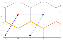
The decision boundary function $f$ for $A_{2}$ is illustrated on Figure 1 by the thick yellow line. This function is the same triangle wave function as the one used to prove the main separation theorem between deep and shallow networks in [Telgarsky2016]. We quickly recall the main ideas of his proof (a more detailed explanation is also available in Appendix LABEL:App_Telgarsky). A triangle wave function $f$ with $p$ periods is considered. It has $2p+1$ affine pieces. Telgarsky established a lower bound of the average pointwise disagreement $|f(\tilde{y})-g(\tilde{y})|$ over a compact set between this function and a function $g$ having $k$ pieces where $k<2p+1$. This is achieved by summing the triangle areas above (resp. below) the dashed black line (see Figure 1 or Figure LABEL:fig_func_Tel) whenever $g$ is below (resp. above) this same line. Indeed, since $g$ has a limited number of pieces, it can only cross this line a limited number of times.

Figure 1: $\mathcal{P}(\mathcal{B})$ for $A_{2}$. The thick blue arrows represent the basis. The CPWL boundary function $f$ defined on $\mathcal{D}(\mathcal{B})$ is illustrated by the thick yellow line. The corner points in $\mathcal{C}^{1}_{\mathcal{P}(\mathcal{B})}$ are in red and the corner points in $\mathcal{C}^{0}_{\mathcal{P}(\mathcal{B})}$ are in black. $f$ can also be extended to a larger compact set (the thin red lines).

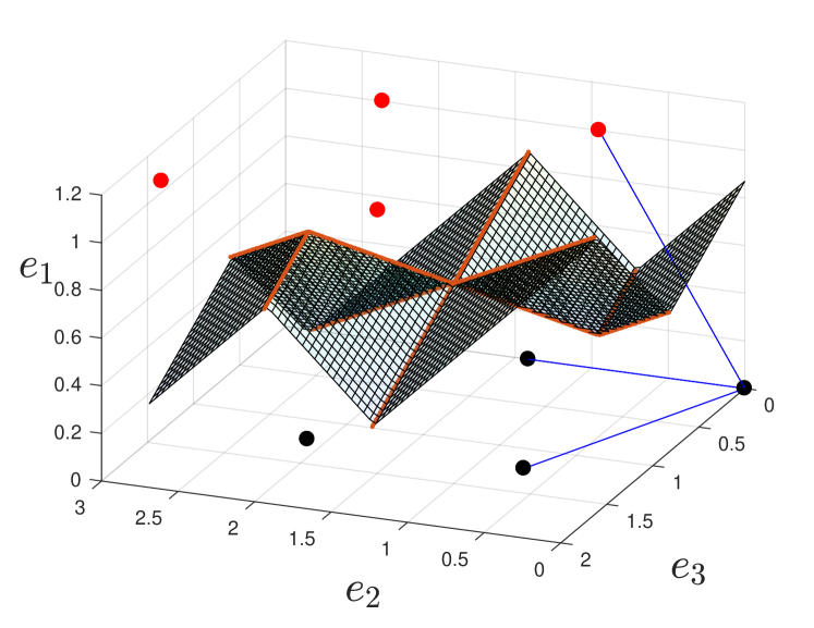
Now, what happens if we consider a similar function in $\mathbb{R}^{3}$, where we replace triangles by tetrahedra? Such a function, limited to $\mathcal{D}(B)$, is illustrated on Figure 3. It is the decision boundary obtained for $A_{3}$ defined by $\eqref{eq_{b}asis_{A}n}$. The dashed line of Figure 1 should now be replaced by the plane $\Phi^{n=3}=\{y\in\mathbb{R}^{3}:\ y\cdot e_{1}=\frac{1}{2}\times(b_{1}\cdot e_{1})\}$. Similarly to the triangle wave function, $f^{n=3}$ is oscillating around $\Phi^{n=3}$: all pieces of $f^{n=3}$ cross $\Phi^{n=3}$. Note that the number of pieces is significantly increased compared to a simple extension of the triangle wave function in $\mathbb{R}^{3}$ (see e.g. Figure LABEL:fig_func_Tel_2). Another figure with $\Phi^{n=3}$ cutting $f^{n=3}$ is available in Appendix LABEL:App_addi_mat. The same pattern is observed for any space dimension $n$, where the triangles or tetrahedra become $n$-simplices.

Figure 2: CPWL decision boundary function for $A_{3}$. The basis vectors are represented by blue lines. The corner points in $\mathcal{C}^{1}_{\mathcal{P}(\mathcal{B})}$ are in red and the corner points in $\mathcal{C}^{0}_{\mathcal{P}(\mathcal{B})}$ in black.

Figure 3: The Voronoi cell of $A_{3}$ is a rhombic dodecahedron. A subset of the facets of this polytope generates some affine pieces of $f$. The non-truncated tetrahedron is the part of the dodecahedron below the plane $\Phi^{n=3}$.

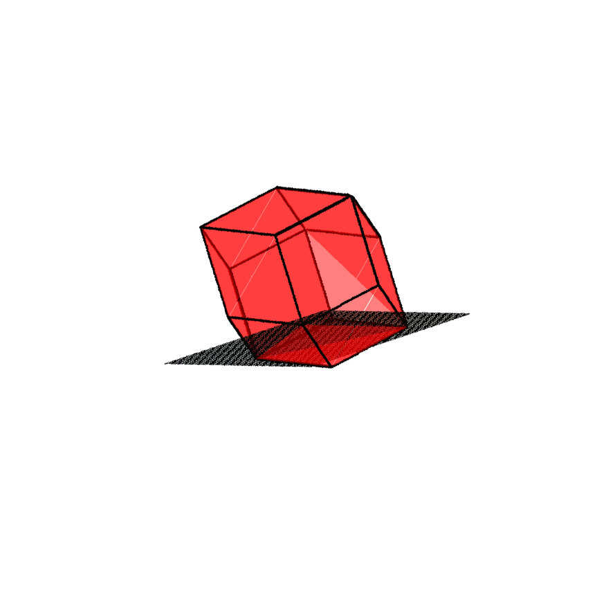
Consider any convex part of $f$, say $f_{m}=\vee_{k=1}^{l_{m}}g_{m,k}$ (see eq_boundary_funct). There are $2^{n-1}$ of such $f_{m}$. The polytope