Interaction-aware Factorization Machines for Recommender Systems

Abstract

Factorization Machine (FM) is a widely used supervised learning approach by effectively modeling of feature interactions. Despite the successful application of FM and its many deep learning variants, treating every feature interaction fairly may degrade the performance. For example, the interactions of a useless feature may introduce noises; the importance of a feature may also differ when interacting with different features. In this work, we propose a novel model named Interaction-aware Factorization Machine (IFM) by introducing Interaction-Aware Mechanism (IAM), which comprises the feature aspect and the field aspect, to learn flexible interactions on two levels. The feature aspect learns feature interaction importance via an attention network while the field aspect learns the feature interaction effect as a parametric similarity of the feature interaction vector and the corresponding field interaction prototype. IFM introduces more structured control and learns feature interaction importance in a stratified manner, which allows for more leverage in tweaking the interactions on both feature-wise and field-wise levels. Besides, we give a more generalized architecture and propose Interaction-aware Neural Network (INN) and DeepIFM to capture higher-order interactions. To further improve both the performance and efficiency of IFM, a sampling scheme is developed to select interactions based on the field aspect importance. The experimental results from two well-known datasets show the superiority of the proposed models over the state-of-the-art methods.

Introduction

Learning the effects of feature conjugations, especially degree-2 interactions, is important for prediction accuracy(?). For instance, people often download apps for food delivery at meal-time, which suggests that the (order-2) interaction between the app category and the time-stamp is an important signal for prediction(?). Applying a linear model on the explicit form of degree-2 mappings can capture the relationship between features, where feature interactions can be easily understood and domain knowledge can be absorbed. The widely used generalized linear models (e.g., logistic regression) with cross features are effective for learning on a massive scale. Although the feature vector might have billions of dimensions, each instance will typically have only hundreds of non-zero values, and FTRL(?) can save both time and memory when making predictions. However, feature engineering is an important but labor-intensive and time-consuming work, and the “cold-start” problem may hurt performance, especially in a sparse dataset, where only a few cross features are observed; the parameters for unobserved cross features cannot be estimated.

To address the generalization issue, factorization machines (FMs)(?) were proposed, which factorizes coefficients into a product of two latent vectors to utilize collaborative information and demonstrate superior performance to a linear model based on the explicit form of degree-2 mappings. In FM, unseen feature interactions can be learned from other pairs, which is useful, as demonstrated by the effectiveness of latent factor models(?; ?). In fact, by specifying the input feature vector, FM can achieve the same express capacity of many factorization models, such as matrix factorization, the pairwise interaction tensor factorization model(?), and SVD++(?).

Despite the successful application of FM, two-folds significant shortcomings still exist. (1) Feature aspect. On one hand, the interactions of a useless feature may introduce noises. On the other hand, treating every feature interaction fairly may degrade the performance. (2) Field aspect. A latent factor may also have different importance in feature interactions from different fields. Assuming that there is a latent factor indicating the quality of a phone, this factor may be more important to the interaction between a phone brand and a location than the interaction between gender and a location. To solve the above problems, we propose a novel model called Interaction-aware Factorization Machine (IFM) to learn flexible interaction importance on both feature aspect and field aspect.

Meanwhile, as a powerful approach to learning feature representation, deep neural networks are becoming increasingly popular and have been employed in predictive models. For example, Wide&Deep(?) extends generalized linear models with a multi-layer perceptron (MLP) on the concatenation of selected feature embedding vectors to learn more sophisticated feature interactions. However, in the wide part of the Wide&Deep model, feature engineering is also required and drastically affects the model performance.

To eliminate feature engineering and capture sophisticated feature interactions, many works(?; ?) are proposed and some of them have fused FM with MLP. FNN(?) initializes parts of the feed-forward neural network with FM pre-trained latent feature vectors, where FM is used as a feature transformation method. PNN(?) imposes a product layer between the embedding layer and the first hidden layer and uses three different types of product operations to enhance the model capacity. Nevertheless, both FNN and PNN capture only high-order feature interactions and ignore low-order feature interactions. DeepFM(?) shares the feature embedding between the FM and deep component to make use of both low- and high-order feature interactions; however, simply concatenating(?; ?) or averaging embedding vectors(?; ?) does not account for any interaction between features. In contrast to that, NFM(?) uses a bi-interaction operation that models the second-order feature interactions to maintain more feature interaction information. Unfortunately, the pooling operation in NFM may also cause information loss. To address this problem, interaction importance on both feature aspect and field aspect is encoded to facilitate the MLP to learn feature interactions more accurately.

The main contributions of the paper include the following:

• To the best of our knowledge, this work represents the first step towards absorbing field information into interaction importance learning.

• The proposed interaction-aware models can effectively learn interaction importance and require no feature engineering.

• The proposed IFM provides insight into which feature interactions contribute more to the prediction at the field level.

• A sampling scheme is developed to further improve both the performance and efficiency of IFM.

• The experimental results on two well-known datasets show the superiority of the proposed interaction-aware models over the state-of-the-art methods.

Factorization Machines

We assume that each instance has attributions $x=\left\{x_{1},x_{2},...,x_{m}\right\}$ from $n$ fields and a target $y$, where $m$ is the number of features and $x_{i}$ is the real valued feature in the $i$-th category. Let $V\text{$\in$}\mathbb{R}^{K\times m}$ be the latent matrix, with column vector $V_{i}$ representing the $K$-dimensional feature-specific latent feature vector of feature $i$. Then pair-wise enumeration of non-zero features can be defined as

$$\mathcal{X}=\{(i,j)\mid 0<i\leq m,0<j\leq m,j>i,x_{i}\neq 0,x_{j}\neq 0\}.$$ (1)

Factorization Machine (FM)(?) is a widely used model that captures all interactions between features using the factorized parameters:

$$\overline{y}=w_{0}+\sum_{i=1}^{m}{w_{i}x_{i}}+\underbrace{\sum_{(i,j)\in\mathcal{X}}w_{ij}x_{i}x_{j}}_{\text{pair-wise feature interactions}}\text{,}$$ (2)

where $w_{0}$ is the global bias, and $w_{i}$ models the strength of the i-th variable. In addition, FM captures pairwise (order-2) feature interactions effectively as $w_{ij}=\langle V_{i},V_{j}\rangle$, where $\langle\cdot{,}\cdot\rangle$ is the inner product of two vectors; therefore, the parameters for unobserved cross features can also be estimated.

Figure 1: The neural network architecture of the proposed Interaction-aware Factorization Machine (IFM).

Proposed Approach

In this section, we first present the interaction-aware mechanism. Subsequently, we detail the proposed Interaction-aware Factorization Machine (IFM). Finally, we propose a generalized interaction-aware model and its neural network specialized versions.

Interaction-Aware Mechanism (IAM)

The pair-wise feature interaction part of FM can be reformulated as

$$\begin{split}\sum_{i=1}^{m}\sum_{j=i+1}^{m}1\cdot\langle\mathbf{1},V_{i}\odot V_{j}\rangle x_{i}x_{j},\\ \end{split}$$ (3)

where $\mathbf{1}$ is a $K$-dimensional vector with all entries one and $\odot$ denotes the Hadamard product. Then we introduce the Interaction-Aware Mechanism (IAM) to discriminate the importance of feature interactions, which simultaneously considers field information as auxiliary information,

$$\sum_{i=1}^{m}\sum_{j=i+1}^{m}T_{ij}\langle\underbrace{F_{f_{i},f_{j}}}_{\text{\clap{field aspect~{}}}},V_{i}\odot V_{j}\rangle x_{i}x_{j}\text{,}$$ (4)

where $f_{i}$ is the field of feature $i$, $F_{f_{i},f_{j}}$ is the $K$-dimensional field-aware factor importance vector of the interaction between feature $i$ and feature $j$ modeling the field aspect; thus, both factors from the same feature interaction and the same factor of interactions from different fields can have significantly different influences on the final prediction. $T_{ij}$ is the corresponding attention score modeling the feature aspect; thus, the importance of feature interactions can be significantly different, which is defined as

$$\begin{split}a_{ij}^{\prime}&=h^{T}\mathrm{Relu}(W(V_{i}\odot V_{j})x_{i}x_{j}+b),\\ T_{ij}&=\frac{\text{exp}(a_{ij}^{\prime}/\tau)}{\sum_{(i,j)\in\mathcal{X}}\text{exp}(a_{ij}^{\prime}/\tau)},\end{split}$$ (5)

where $K_{a}$ is the hidden layer size of the attention network, $b\text{$\in$}\mathbb{R}^{K_{a}}$, $h\text{$\in$}\mathbb{R}^{K_{a}}$, $W\text{$\in$}\mathbb{R}^{K_{a}\times K}$, and $\tau$ is a hyperparameter that was originally used to control the randomness of predictions by scaling the logits before applying softmax(?). Here we use $\tau$ to control the effectiveness strength of the feature aspect. For a high temperature($\tau\to\infty$), all interactions have nearly the same importance, and the feature aspect has a limited impact on the final prediction. For low temperatures ($\tau\to 0$), the probability of the interaction vector with the highest expected reward tends to 1 and the other interactions are ignored.

The raw presentation of $F$ has $n(n-1)/2\times K$ parameters, where $n$ is the number of fields, so the space complexity of IAM is quadratic in the field number. We further factorize tensor $F$ using canonical decomposition(?):

$$F_{f_{i},f_{j}}=D^{T}(U_{f_{i}}\odot U_{f_{j}})\text{,}$$ (6)

where $U\text{$\in$}\mathbb{R}^{K_{F}\times n}$ and $D\text{$\in$}\mathbb{R}^{K_{F}\times K}$, and $K_{F}$ is the number of latent factors of both $U$ and $D$. Therefore, the space complexity is reduced to $O(nK_{F}+K_{F}K)$, which is linear in the field number.

From another perspective, field aspect learns feature interaction effect as a parametric similarity of the feature interaction vector $(V_{i}\odot V_{j})x_{i}x_{j}$ and the corresponding field interaction prototype $U_{f_{i}}\odot U_{f_{j}}$, which has a bi-linear form(?),

$$sim_{D}(c,e)=c^{T}De\text{,}$$ (7)

with $c=U_{f_{i}}\odot U_{f_{j}}$, $e=(V_{i}\odot V_{j})x_{i}x_{j}$.

Interaction-aware Factorization Machines (IFMs)

Interaction-aware Factorization Machine (IFM) models feature interaction importance more precisely by introducing IAM. For simplicity, we omit linear terms and the bias term in the remaining parts. Figure 1 shows the neural network architecture of IFM, which comprises 6 layers. In the following, several layers are detailed:

• Embedding layer. The embedding layer is a fully connected layer that projects each feature to a dense vector representation. IFM employs two embedding matrices $V$ and $U$ for feature embedding and field embedding querying, respectively.

• Pair-wise interaction layer. The pair-wise interaction layer enumerates interacted latent vectors, each of which is a element-wise product of two embedding vectors from the embedding layer. Let the feature aspect pair-wise interaction set $\mathcal{P}_{F}$ and the field aspect pair-wise interaction set $\mathcal{P}_{I}$ be

  $$\mathcal{P}_{F} =\{(V_{i}\odot V_{j})x_{i}x_{j}\mid(i,j)\text{$\in$}\mathcal{X}\},$$ (8)

  $$\mathcal{P}_{I} =\{U_{f_{i}}\odot U_{f_{j}}\mid(i,j)\text{$\in$}\mathcal{X}\},$$

  then each has no information overlap; the former only depends on the feature embedding matrix $V$, while the latter only comes from the field embedding matrix $U$.

• Inference layer. The inference layer calculates the feature aspect importance and the field aspect importance according to Equation 5 and Equation 6, respectively.

To summarize, we give the overall formulation of IFM as:

$$\overline{y}=\sum_{i=1}^{m}\sum_{j=i+1}^{m}T_{ij}(U_{f_{i}}\odot U_{f_{j}})^{T} D(V_{i}\odot V_{j})x_{i}x_{j}$$ (9)

$$+ \sum_{i=1}^{m}{w_{i}x_{i}}+w_{0}\text{.}$$

We also apply $L_{2}$ regularization on $U$ and $D$ with $\lambda_{F}$ controling the regularization strength and employ dropout(?) on the pair-wise interaction layer to prevent overfitting. Note that $U\text{$\in$}\mathbb{R}^{K_{F}\times n}$ and $V\text{$\in$}\mathbb{R}^{K\times m}$ can have different dimensions; each latent vector of $U$ only needs to learn the effect with a specific field, so usually,

$$K_{F}\ll K.$$ (10)

Complexity Analysis. Feature embedding matrix $V$ require $m\times K$ parameters and field-aware factor importance matrix $F$ requires $n\times K_{F}+K_{F}\times K$ parameters after applying Equation 6. Besides, the parameters of attention network is $K_{a}\times K+2K_{a}$. Thus, the overall space complexity is $O(nK_{F}+(K_{F}+m+K_{a})K+2K_{a})$, where $K_{F},K_{a},K$ and $n$ are small compared to $m$, so the space complexity is similar to that of FM, which is $O(mK)$.

The cost of computing $\mathcal{P}_{F}$ (Equation 8) and feature aspect importance are $O(|\mathcal{X}|K)$ and $O(|\mathcal{X}|KK_{a})$, respectively. For prediction, because the field-aware factor importance matrix $F$ can be pre-calculated by Equation 6 and the fusion layer only involves the inner product of two vectors, for which the complexity is $O(|\mathcal{X}|K)$, the overall time complexity is $O(|\mathcal{X}|KK_{a})$.

Sampling. We dynamically sample $c$ feature interactions according to the norms of field-aware factor importance vectors ($F_{f_{i},f_{j}}$) and attention scores are only computed for the sampled interactions. The cost of sampling is $O(n^{2}K_{F}K)$ for a mini-batch data and the computation cost of attention scores is $O(cKK_{a})$ for every instance. By sampling, the selection frequency for useless interactions is reduced and the overall time complexity is reduced to $O(cKK_{a}+\frac{n^{2}}{batchSize}K_{F}K)$.

Generalized Interaction-aware Model (GIM)

We present a more generalized architecture named Generalized Interaction-aware Model (GIM) in this section and derive its neural network versions to effectively learn higher order interactions. Let feature aspect embedding set $\mathcal{F_{X}}$ and field aspect embedding set $\mathcal{I_{X}}$ be

$$\begin{split}\mathcal{F_{X}}&=\{T_{ij}V_{i}\odot V_{j}x_{i}x_{j}\mid(i,j)\text{$\in$}\mathcal{X}\},\\ \mathcal{I_{X}}&=\{D^{T}(U_{f_{i}}\odot U_{f_{j}})\mid(i,j)\text{$\in$}\mathcal{X}\},\end{split}$$ (11)

Then, the final prediction can be calculated by introducing function $G$ as

$$\overline{y}=G(\mathcal{F_{X}},\mathcal{I_{X}}).$$ (12)

Let $\mathcal{F_{X}}_{i,j}$ and $\mathcal{I_{X}}_{i,j}$ be the element with index $(i,j)$ in $\mathcal{F_{X}}$ and $\mathcal{I_{X}}$, respectively. Then IFM can be seen as a special case of GIM using the following,

$$G_{IFM}(\mathcal{F_{X}},\mathcal{I_{X}})=\sum\{\mathcal{I_{X}}_{i,j}^{T}\mathcal{F_{X}}_{i,j}\mid(i,j)\text{$\in$}\mathcal{X}\}.$$ (13)

Besides, $G$ can be a more complex function to capture the non-linear and complex inherent structure of real-world data. Let

$$\begin{split}h^{0}=&\mathop{concate}\{\mathcal{I_{X}}_{i,j}\odot\mathcal{F_{X}}_{i,j}\mid(i,j)\text{$\in$}\mathcal{X}\},\\ h_{l}=&f_{l}(Q_{l}h_{l-1}+z_{l}),\\ \end{split}$$ (14)

where $n_{l}$ is the number of nodes in the $l$-th hidden layer; then, $Q_{l}\text{$\in$}\mathbb{R}^{n_{l}\times n_{l-1}}$, $z_{l}\text{$\in$}\mathbb{R}^{n_{l}}$ are parameters for the $l$-th hidden layer, $f_{l}$ is the activation function for the $l$-th hidden layer, and $h_{l}\text{$\in$}\mathbb{R}^{n_{l}}$ is the output of the $l$-th hidden layer. Specially, Interaction-aware Neural Network (INN) is defined as

$$G_{INN}(\mathcal{F_{X}},\mathcal{I_{X}})=h_{L},$$ (15)

where $L$ denotes the number of hidden layers and $f_{L}$ is the identity function. For hidden layers, we use $\mathrm{Relu}$ as the activation function, which empirically shows good performance.

To learn both high- and low-order feature interactions, the wide component of DeepFM(?) is replaced by $G_{IFM}(\mathcal{F_{X}},\mathcal{I_{X}})$ and named as DeepIFM.

Experimental results

In this section, we evaluate the performance of the proposed IFM, INN and DeepIFM on two real-world datasets and examine the effect of different parts of IFM. We conduct experiments with the aim of answering the following questions:

• RQ1 How do IFM and INN perform compared to the state-of-the-art methods?

• RQ2 How do the feature aspect and the field aspect (with sampling) impact the prediction accuracy?

• RQ3 How dose factorization of field-aware factor importance matrix $F$ impact the performance of IFM?

• RQ4 How do the hyper-parameters of IFM impact its performance?

Experiment Settings

Datasets and Evaluation. We evaluate our models on two real-world datasets, MovieLens(?) and Frappe(?), for personalized tag recommendation and context-aware recommendation. We follow the experimental settings in the previous works(?; ?) and use the optimal parameter settings reported by the authors to have fair comparisons. The datasets are divided into a training set (70%), a probe set (20%), and a test set (10%). All models are trained on the training set, and the optimal parameters are obtained on the held-out probe set. The performance is evaluated by the root mean square error (RMSE), where a lower score indicates better performance, on the test set with the optimal parameters. Both datasets contain only positive records, so we generate negative samples by randomly pairing two negative samples with each log and converting each log into a feature vector via one-hot encoding. Table 1 shows a description of the datasets after processing, where the sparsity level is the ratio of observed to total features(?).

Table 1: Dataset Description.

Data set	MovieLens	Frappe
origin records	668,953	96,203
features	90,445	5,382
experimental records	2,006,859	288,609
fields	3	10
sparsity level	0.01%	0.19%

Baselines. We compare our models with the following methods:

• FM(?). As described in Equation 2. In addition, dropout is employed on the feature interactions to further improve its performance.

• FFM(?). Each feature has separate latent vectors to interact with features from different fields.

• AFM(?). AFM learns one coefficient for every feature interaction to enable feature interactions that contribute differently to the prediction.

• Neural Factorization Machines (NFMs)(?). NFM performs a non-linear transformation on the latent space of the second-order feature interactions. Batch normalization(?) is also employed to address the covariance shift issue.

• DeepFM(?). DeepFM shares the feature embedding between the FM and the deep component.

Regularization. We use $L_{2}$ regularization, dropout, and early stopping.

Hyperparameters. The model-independent hyperparameters are set to the optimal values reported by the previous works(?; ?). The embedding size of features is set to 256, and the batch size is set to 4096 and 128 for MovieLens and Frappe, respectively. We also pre-train the feature embeddings with FM to get better results. For IFM and INN, we set $\tau=10$ and tune the other hyperparameters on the probe set.

Model Performance (RQ1)

The performance of different models on the MovieLens dataset and the Frappe dataset is shown in Table 2, from which the following observations may be made:

• Learning the importance of different feature interactions improves performance. This observation is derived from the fact that both AFM and the IAM-based models (IFM and INN) perform better than FM does. As the best model, INN outperforms FM by more than 10% and 7% on the MovieLens and Frappe datasets, respectively.

• IFM makes use of field information and can model feature interactions more precisely. To verify the effectiveness of field information, we conduct experiments with FFM and FFM-style AFM, where each feature has separate latent vectors to interact with features from different fields, on the MovieLens dataset. As expected, the utilization of field information brings improvements of approximately 2% and 3% with respect to FM and AFM.

• INN outperforms IFM by using a more complex function $G$, as described in Equation 15, which captures more complex and non-linear relations from IAM encoded vectors.

• Overall, our proposed IFM model outperforms the competitors by more than 4.8% and 1.2% on the MovieLens and Frappe datasets, respectively. The proposed INN model performs even better, which achieves an improvement of approximately 6% and 1.5% on the MovieLens and Frappe datasets, respectively.

Table 2: Test RMSE from different models.

	Frappe		MovieLens
Method	#Param	RMSE	#Param	RMSE
FM	1.38M	0.3321	23.24M	0.4671
DeepFM	1.64M	0.3308	23.32M	0.4662
FFM	13.8M	0.3304	69.55M	0.4568
NFM	1.45M	0.3171	23.31M	0.4549
AFM	1.45M	0.3118	23.25M	0.4430
IFM-sampling	1.46M	0.3085	-	-
IFM	1.46M	0.3080	23.25M	0.4213
INN	1.46M	0.3071	23.25M	0.4188

Impact of different aspects and sampling (RQ2)

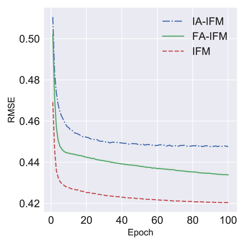
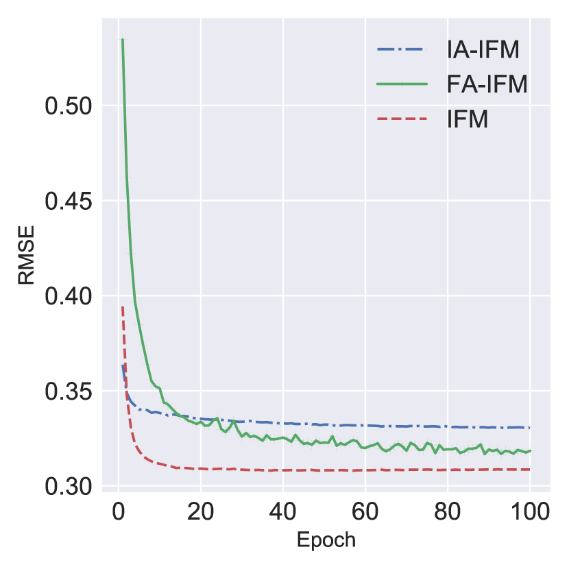
IFM discriminates feature interaction importance on feature aspect and field aspect. To study how each aspect influences IFM prediction, we keep only one aspect and monitor how IFM performs. As shown in Figure 2, feature-aspect-only IFM (FA-IFM) performs better than field-aspect-only IFM (IA-IFM) does. We explain this phenomenon by examining the models. The FA-IFM modeling of feature interaction importance is more detailed for each individual interacted vectors; thus, it can make use of the feature interaction information precisely, whereas IA-IFM utilizes only field-level interaction information and lacks the capacity to distinguish feature interactions from the same fields. Although FA-IFM models feature interactions in a more precise way, IFM still achieves a significant improvement by incorporating field information, which can be seen as auxiliary information, to give more structured control and allow for more leverage when tweaking the interaction between features.

We now focus on analyzing the different role of field aspect in different datasets. We calculated the ratio of the improvements of FA-IFM over IA-IFM, which were 9:1 and 1.7:1 on the Frappe and MovieLens datasets, respectively. It is determined that field information plays a more significant role in the MovieLens dataset. We explain this phenomenon by examining the datasets. As shown in Table 1, the MovieLens dataset is sparser than the Frappe dataset, where the field information brings more benefit(?).

Field importance Analysis. Field aspect not only improves the model performance but also gives the ability to interpret the importance of feature interactions at the field-factor level. Besides, the norm of field aspect importance vector provides insight into interaction importance at the field level. To demonstrate this, we investigate field aspect importance vectors on the MovieLens dataset. As shown in Table 3, the movie-tag interaction is the most important while the user-movie interaction has a negligible impact on the prediction because tags link users and items as a bridge(?) and directly modeling semantic correlation between them is less effective.

Sampling. To examine how sampling affects the performance of IFM, an experiment was conducted on Frappe dataset and because there are only three interactions in MovieLens dataset, sampling is meaningless. As shown in Table 2, IFM with sampling achieves a similar level of performance. To verify how sampling performs when the dataset is large, we compare the performance on click-through prediction for advertising in Tencent video, which has around 10 billion instances. As shown in Table 4, sampling reduce the training time with no significant loss to the performance.

Table 3: The norm of field aspect importance vector of each feature interaction on the MovieLens dataset.

	User-Movie	User-Tag	Movie-Tag
norm	0.648	5.938	9.985
proportion	3.9 %	35.8 %	60.3 %

Table 4: The performance on click-through prediction for advertising in Tencent video.

Method	AUC	Time
DeepIFM	0.8436	16hrs, 18mins
DeepIFM-Sampling(10%)	0.8420	3hrs, 49mins

(a) MovieLens

(b) Frappe

Figure 2: Comparison of test RMSE by using only one aspect.

Impact of factorization (RQ3)

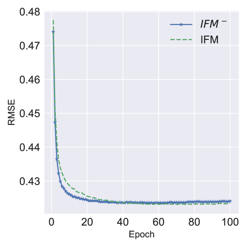
As described in Equation 6, IAM factorizes field-aware factor importance matrix $F\text{$\in$}\mathbb{R}^{n(n-1)/2\times K}$ to get a more compact representation. We conduct experiments with both the factorized version and the non-factorized version (indicated as IFM^-) to determine how factorization affects the performance. As shown in Figure 3, factorization can speed up the convergence of both datasets. However, it also has a significantly different impact on the performance of the two datasets. For the MovieLens dataset, both versions achieve similar levels of performance but IFM outperforms IFM^- by a large margin on the Frappe dataset, where the performance of IFM^- is degraded from epoch 50 because of an overfitting issue. We explain this phenomenon by comparing the number of entries of field-aware factor importance matrix $F$. For the Frappe dataset, IFM^- and IFM have 11,520 and 6,370 entries with the optimal settings with $K=256$ and $K_{F}=26$, respectively. That is, after factorization, we can reduce more than 44% of the parameters, thereby significantly reducing the model complexity. In contrast to that, the MovieLens dataset contains only three interactions, where the effect of factorization is negligible and IFM^- performs slightly better than IFM does although the gap is negligible, i.e., around 0.1%.

(a) MovieLens

(b) Frappe

Figure 3: Performance comparison on the test set w.r.t. IFM and the non-factorization version IFM-.

Effect of Hyper-parameters (RQ4)

(a) MovieLens

(b) Frappe

Figure 4: Comparison of test RMSE by varying keep probabilities.

(a) MovieLens

(b) Frappe

Figure 5: Comparison of test RMSE by varying $\lambda_{F}$.

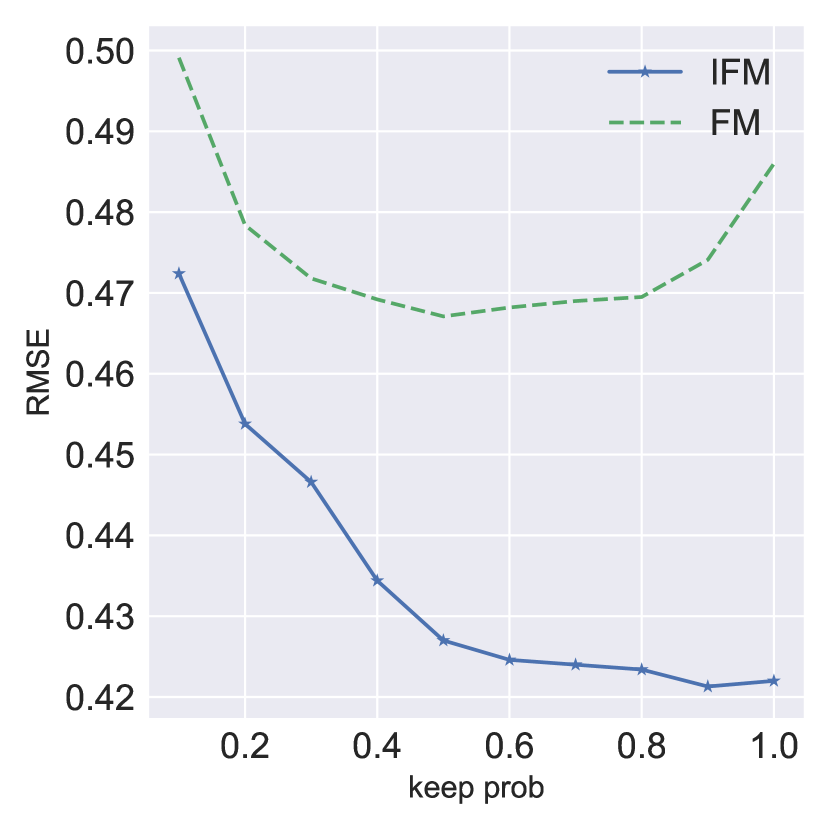
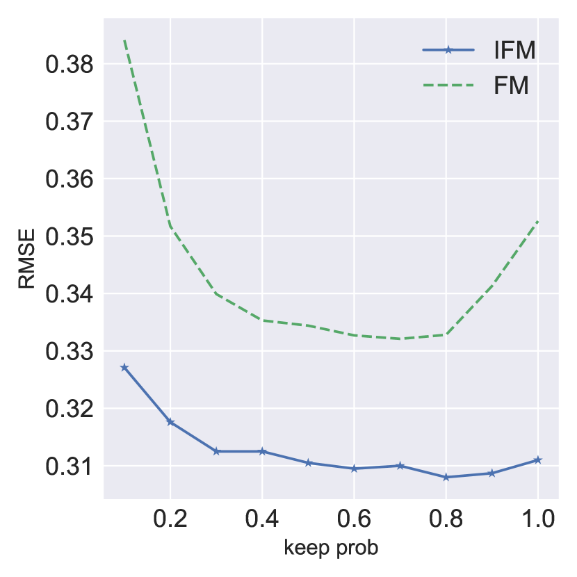
Dropout. Dropout can be seen as a model averaging approach to reduce overfitting by preventing complex co-adaptations on training data. We apply dropout to FM on feature interaction vectors and obtain better performance as a benchmark. As shown in Figure 4, we set the keep probability from 0.1 to 1.0 with increments of 0.1 and it significantly affects the performance of both FM and IFM. When the keep probability tends to zero, the performance of both models is poor due to the underfitting issue. When the keep probability tends to 1, i.e., no dropout is employed, both models also cannot achieve the best performance. Both IFM and FM achieve the best performance when the keep probability is properly set due to the extreme bagging effect. For nearly all keep probabilities, IFM outperforms FM, which shows the effectiveness of IAM.

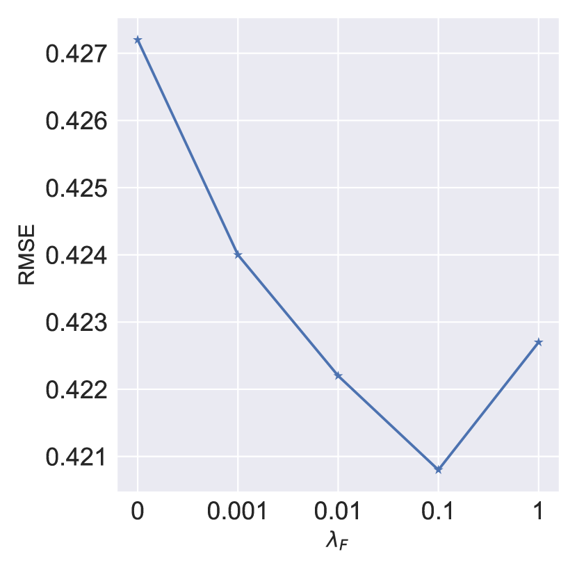
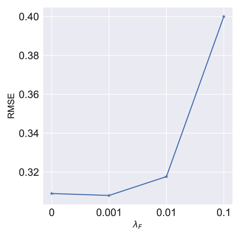
$L_{2}$ regularization. Figure 5 shows how IFM performs when the $L_{2}$ regularization hyperparameter $\lambda_{F}$ varies while keeping the dropout ratio constant (optimal value from the validation dataset). IFM performs better when $L_{2}$ regularization is applied and it achieves an improvement of approximately 1.4% in the MovieLens dataset. We explain this phenomenon as the following. Using dropout on the pair-wise interaction layer only prevent overfitting for the feature aspect and $\lambda_{F}$ controls the regularization strength of factorization parameters for the field aspect importance learning.

(a) MovieLens

(b) Frappe

Figure 6: Comparison of test RMSE by varying $K_{F}$.

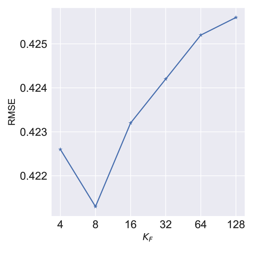
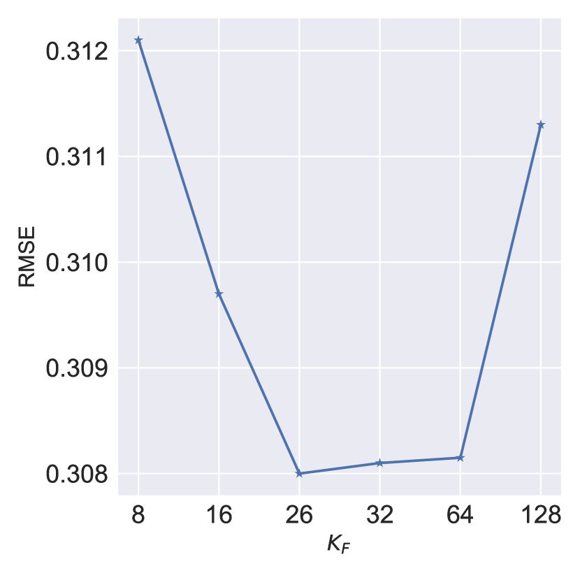
The number of hidden factors $K_{F}$. Figure 6 shows how IFM performs when the number of hidden factors $K_{F}$ varies. IFM cannot effectively capture the field-aware factor importance when $K_{F}$ is small and it also can not achieve the best performance when $K_{F}$ is large due to the overfitting issue. An interesting phenomenon is that the best $K_{F}$ for the MovieLens dataset is much smaller than that for the Frappe dataset. We explain this phenomenon by looking into the datasets. Because the number of fields $n$ is 10 for the Frappe dataset, the field-aware factor importance matrix captures the importance of factors from 45 interacted vectors. While the MovieLens dataset contains only 3 interactions and the field-aware factor importance matrix keeps much less information.

Related work

In the introduction section, factorization machine and its many neural network variants are already mentioned, thus we do not discuss them here. In what follows, we briefly recapitulate the two most related models, i.e., AFM(?) and FFM(?).

AFM learns one coefficient for every feature interaction to enable feature interactions that contribute differently to the final prediction and the importance of a feature interaction is automatically learned from data without any human domain knowledge. However, the pooling layer of AFM lacks the capacity of discriminating factor importance in feature interactions from different fields. In contrast, IFM models feature interaction importance at interaction-factor level; thus, the same factor in different interactions can have significantly different influences on the final prediction.

In FMs, every feature has only one latent vector to learn the latent effect with any other features. FFM utilizes field information as auxiliary information to improve model performance and introduces more structured control. In FFM, each feature has separate latent vectors to interact with features from different fields, thus the effect of a feature can differ when interacting with features from different fields. However, modeling feature interactions without discriminating importance is unreasonable. IFM learns flexible interaction importance and outperforms FFM by more than 6% and 7% on the Frappe and MovieLens datasets, respectively. Moreover, FFM requires $O(mnK)$ parameters, while the space complexity of IFM is $O(mK)$.

Conclusion and Future Directions

In this paper, we proposed a generalized interaction-aware model and its specialized versions to improve the representation ability of FM. They gain performance improvement based on the following advantages. (1) All models can effectively learn both the feature aspect and the field aspect interaction importance. (2) All models can utilize field information that is usually ignored but useful. (3) All models apply factorization in a stratified manner. (4) INN and DeepIFM can learn jointly with deep representations to capture the non-linear and complex inherent structure of real-world data.

The experimental results on two well-known datasets show the superiority of the proposed models over the state-of-the-art methods. To the best of our knowledge, this work represents the first step towards absorbing field information into feature interaction importance learning.

In the future, we would like to generalize the field-aware importance matrix to a more flexible structure by applying neural architecture search(?).

References

- [Baltrunas et al. 2015] Baltrunas, L.; Church, K.; Karatzoglou, A.; and Oliver, N. 2015. Frappe: Understanding the usage and perception of mobile app recommendations in-the-wild. arXiv preprint arXiv:1505.03014.
- [Cao et al. 2016] Cao, B.; Zhou, H.; Li, G.; and Yu, P. S. 2016. Multi-view machines. In Proceedings of the Ninth ACM International Conference on Web Search and Data Mining, 427–436. ACM.
- [Chang et al. 2010] Chang, Y.-W.; Hsieh, C.-J.; Chang, K.-W.; Ringgaard, M.; and Lin, C.-J. 2010. Training and testing low-degree polynomial data mappings via linear svm. Journal of Machine Learning Research 11(Apr):1471–1490.
- [Chechik et al. 2010] Chechik, G.; Sharma, V.; Shalit, U.; and Bengio, S. 2010. Large scale online learning of image similarity through ranking. Journal of Machine Learning Research 11(Mar):1109–1135.
- [Chen et al. 2014] Chen, C.; Zheng, X.; Wang, Y.; Hong, F.; Lin, Z.; et al. 2014. Context-aware collaborative topic regression with social matrix factorization for recommender systems. In AAAI, 9–15.
- [Chen et al. 2016] Chen, C.; Zheng, X.; Wang, Y.; Hong, F.; Chen, D.; et al. 2016. Capturing semantic correlation for item recommendation in tagging systems. In AAAI, 108–114.
- [Chen et al. 2017] Chen, J.; Zhang, H.; He, X.; Nie, L.; Liu, W.; and Chua, T.-S. 2017. Attentive collaborative filtering: Multimedia recommendation with item-and component-level attention. In Proceedings of the 40th International ACM SIGIR conference on Research and Development in Information Retrieval, 335–344. ACM.
- [Cheng et al. 2016] Cheng, H.-T.; Koc, L.; Harmsen, J.; Shaked, T.; Chandra, T.; Aradhye, H.; Anderson, G.; Corrado, G.; Chai, W.; Ispir, M.; et al. 2016. Wide & deep learning for recommender systems. In Proceedings of the 1st Workshop on Deep Learning for Recommender Systems, 7–10. ACM.
- [Guo et al. 2017] Guo, H.; Tang, R.; Ye, Y.; Li, Z.; and He, X. 2017. Deepfm: a factorization-machine based neural network for ctr prediction. In Proceedings of the 26th International Joint Conference on Artificial Intelligence, 1725–1731. AAAI Press.
- [Harper and Konstan 2015] Harper, F. M., and Konstan, J. A. 2015. The movielens datasets: History and context. ACM Transactions on Interactive Intelligent Systems (TiiS) 5(4):19.
- [He and Chua 2017] He, X., and Chua, T.-S. 2017. Neural factorization machines for sparse predictive analytics. In Proceedings of the 40th International ACM SIGIR conference on Research and Development in Information Retrieval, 355–364. ACM.
- [Hinton, Vinyals, and Dean 2015] Hinton, G.; Vinyals, O.; and Dean, J. 2015. Distilling the knowledge in a neural network. arXiv preprint arXiv:1503.02531.
- [Hong, Zheng, and Chen 2016] Hong, F.-X.; Zheng, X.-L.; and Chen, C.-C. 2016. Latent space regularization for recommender systems. Information Sciences 360:202–216.
- [Ioffe and Szegedy 2015] Ioffe, S., and Szegedy, C. 2015. Batch normalization: Accelerating deep network training by reducing internal covariate shift. In International Conference on Machine Learning, 448–456.
- [Juan et al. 2016] Juan, Y.; Zhuang, Y.; Chin, W.-S.; and Lin, C.-J. 2016. Field-aware factorization machines for ctr prediction. In Proceedings of the 10th ACM Conference on Recommender Systems, 43–50. ACM.
- [Kolda and Bader 2009] Kolda, T. G., and Bader, B. W. 2009. Tensor decompositions and applications. SIAM review 51(3):455–500.
- [Koren 2008] Koren, Y. 2008. Factorization meets the neighborhood: a multifaceted collaborative filtering model. In Proceedings of the 14th ACM SIGKDD international conference on Knowledge discovery and data mining, 426–434. ACM.
- [Lee, Sun, and Lebanon 2012] Lee, J.; Sun, M.; and Lebanon, G. 2012. A comparative study of collaborative filtering algorithms. arXiv preprint arXiv:1205.3193.
- [Liu et al. 2017] Liu, C.; Zoph, B.; Shlens, J.; Hua, W.; Li, L.-J.; Fei-Fei, L.; Yuille, A.; Huang, J.; and Murphy, K. 2017. Progressive neural architecture search. arXiv preprint arXiv:1712.00559.
- [McMahan et al. 2013] McMahan, H. B.; Holt, G.; Sculley, D.; Young, M.; Ebner, D.; Grady, J.; Nie, L.; Phillips, T.; Davydov, E.; Golovin, D.; et al. 2013. Ad click prediction: a view from the trenches. In Proceedings of the 19th ACM SIGKDD international conference on Knowledge discovery and data mining, 1222–1230. ACM.
- [Qu et al. 2016] Qu, Y.; Cai, H.; Ren, K.; Zhang, W.; Yu, Y.; Wen, Y.; and Wang, J. 2016. Product-based neural networks for user response prediction. In Data Mining (ICDM), 2016 IEEE 16th International Conference on, 1149–1154. IEEE.
- [Rendle and Schmidt-Thieme 2010] Rendle, S., and Schmidt-Thieme, L. 2010. Pairwise interaction tensor factorization for personalized tag recommendation. In Proceedings of the third ACM international conference on Web search and data mining, 81–90. ACM.
- [Rendle 2010] Rendle, S. 2010. Factorization machines. In Data Mining (ICDM), 2010 IEEE 10th International Conference on, 995–1000. IEEE.
- [Srivastava et al. 2014] Srivastava, N.; Hinton, G.; Krizhevsky, A.; Sutskever, I.; and Salakhutdinov, R. 2014. Dropout: A simple way to prevent neural networks from overfitting. The Journal of Machine Learning Research 15(1):1929–1958.
- [Wang et al. 2015] Wang, P.; Guo, J.; Lan, Y.; Xu, J.; Wan, S.; and Cheng, X. 2015. Learning hierarchical representation model for nextbasket recommendation. In Proceedings of the 38th International ACM SIGIR conference on Research and Development in Information Retrieval, 403–412. ACM.
- [Wang et al. 2017] Wang, R.; Fu, B.; Fu, G.; and Wang, M. 2017. Deep & cross network for ad click predictions. In Proceedings of the ADKDD’17, 12. ACM.
- [Xiao et al. 2017] Xiao, J.; Ye, H.; He, X.; Zhang, H.; Wu, F.; and Chua, T.-S. 2017. Attentional factorization machines: Learning the weight of feature interactions via attention networks. In Proceedings of the Twenty-Sixth International Joint Conference on Artificial Intelligence (IJCAI-17). Morgan Kaufmann.
- [Zhang, Du, and Wang 2016] Zhang, W.; Du, T.; and Wang, J. 2016. Deep learning over multi-field categorical data. In European conference on information retrieval, 45–57. Springer.