Averaging method for dynamic systems
on time scales with periodicity

Abstract.

This paper aims to improve existing results about using averaging method for analysis of dynamic systems on time scales. We obtain a more accurate estimate for proximity between solutions of original and averaged systems regarding $\Delta$–periodic and $\Delta$-quasiperiodic systems, which are introduced for the first time. To illustrate the application of the averaging theorem for such kind of system we considered an example and conducted numerical modelling. Obtained results extend an application area for previously developed numerically–asymptotic method of solution for optimal control problems on time scales.

1. Introduction

A systematic theory of averaging method for ordinary differential equations began from the works of [Krylov and Bogolyubov(1947)]. Further it was developing by [Bogolyubov and Mitropol’skii(1961)] and the others. Since then, there have been many works establishing the averaging method for various types of dynamic systems: differential equations with discontinuous and multi-valued right-hand side, with Hukuhara derivative, with delay etc. The review of these results one can find in [Plotnikov(1992)].

On the other hand, the theory of dynamic equations on time scales was introduced by [Hilger(1988)] in order to unify continuous and discrete calculus. In detail, the description of time scale analysis can be found in the [Bohner and Peterson(2012), Bohner and Peterson(2002)].

As far as we know the averaging method in connection with the systems on time scales was first examined by [Slavík(2012)]. In particular, there were studied conditions of proximity between solutions of the original system on time scale and some generalized differential equation. From the practical point of view, the interpretation of the last equation’s solution in terms of given application is somewhat unclear.

Previously we established the scheme of full averaging for dynamic systems on time scales ([Ogulenko and Kichmarenko(2012)]) and in our approach the averaged system has the same time nature as the original one. Recently we also established the analogous result for partially averaged systems, [Ogulenko(2017)]. On the base of this scheme, it was developed the numerically–asymptotic method of solution for optimal control problems on time scales ([Ogulenko and Kichmarenko(2016), Kichmarenko and Ogulenko(2017)]).

2. Preliminary results.

We now present some basic information about time scales according to [Bohner and Peterson(2012)]. A time scale is defined as a nonempty closed subset of the set of real numbers and usually denoted by $\mathbb{T}$. The properties of the time scale are determined by the following three functions: 1) the forward-jump operator $\sigma(t)=\inf\left\{s\in\mathbb{T}:s>t\right\}$; 2) the backward-jump operator $\rho(t)=\sup\left\{s\in\mathbb{T}:s<t\right\}$ (in this case, we set $\inf\varnothing=\sup\mathbb{T}$ and $\sup\varnothing=\inf\mathbb{T}$); 3) the granularity function $\mu(t)=\sigma(t)-t$.

The behaviour of the forward- and backward-jump operators at a given point of the time scale specifies the type of this point. If $t<\sigma(t)$, then $t$ is called right–scattered, if $t=\sigma(t)$ — right–dense. Also, point will be called left–scattered when $\rho(t)<t$ and left–dense when $\rho(t)=t$. Finally, point is called dense if it is right-dense and left–dense at the same time and isolated if it is both right–scattered and left-scattered.

Important role in time scales calculus has the set $\mathbb{T}^{\kappa}$ which is derived from the time scale $\mathbb{T}$ as follows: if $\mathbb{T}$ has a left–scattered maximum $m$, then $\mathbb{T}^{\kappa}=\mathbb{T}-\{m\}$. Otherwise, $\mathbb{T}^{\kappa}=\mathbb{T}$. In what follows, we set $\left[a,b\right]_{\mathbb{T}}=\left\{t\in\mathbb{T}:a\leqslant t\leqslant b\right\}$.

Definition 1 ([Bohner and Peterson(2012)]).

Let $f:\mathbb{T}\rightarrow\mathbb{R}$ and $t\in\mathbb{T}^{\kappa}$. The number $f^{\Delta}(t)$ is called $\Delta$-derivative of function $f$ at the point $t$, if $\forall\varepsilon>0$ there exists a neighborhood $U$ of the point $t$ (i. e., $U=(t-\delta,t+\delta)\cap\mathbb{T},\delta<0$) such that

$$\lvert f(\sigma(t))-f(s)-f^{\Delta}(t)(\sigma(t)-s)\rvert\leqslant\varepsilon\lvert\sigma(t)-s\rvert\quad\forall s\in U.$$

Definition 2 ([Bohner and Peterson(2012)]).

If $f^{\Delta}(t)$ exists $\forall t\in\mathbb{T}^{\kappa}$, then $f:\mathbb{T}\rightarrow\mathbb{R}$ is called $\Delta$-differentiable on $\mathbb{T}^{\kappa}$. The function $f^{\Delta}(t):\mathbb{T}^{\kappa}\rightarrow\mathbb{R}$ is called the delta-derivative of a function $f$ on $\mathbb{T}^{\kappa}$.

If $f$ is differentiable with respect to $t$, then $f(\sigma(t))=f(t)+\mu(t)f^{\Delta}(t)$.

Definition 3 ([Bohner and Peterson(2012)]).

The function $f:\mathbb{T}\rightarrow\mathbb{R}$ is called $rd$-continuous if it is continuous at the right-dense points and has finite left limits at the left-dense points. The set of these functions is denoted by $C_{rd}=C_{rd}(\mathbb{T})=C_{rd}(\mathbb{T};\mathbb{R})$.

The indefinite integral on the time scale takes the form $\int{f(t)\Delta t}=F(t)+C$, where $C$ is integration constant and $F(t)$ is the preprimitive for $f(t)$. If the relation $F^{\Delta}(t)=f(t)$ where $f:\mathbb{T}\rightarrow\mathbb{R}$ is an $rd$-continuous function, is true for all $t\in\mathbb{T}^{\kappa}$ then $F(t)$ is called the primitive of the function $f(t)$. If $t_{0}\in\mathbb{T}$ then $F(t)=\int\limits_{t_{0}}^{t}{f(s)\Delta s}$ for all $t$. The definite $\Delta$-integral on time scale interval is defined by Newton–Leibniz formula.

Definition 4 ([Bohner and Peterson(2012)]).

A function $p:\mathbb{T}\rightarrow\mathbb{R}$ is called regressive (positive regressive) if

$$1+\mu(t)p(t)\neq 0,\quad(1+\mu(t)p(t)>0),\qquad t\in\mathbb{T}^{\kappa}.$$

The set of regressive (positive regressive) and $rd$-continuous functions is denoted by $\mathcal{R}=\mathcal{R}(\mathbb{T})$ ($\mathcal{R}^{+}=\mathcal{R}^{+}(\mathbb{T})$).

A function $p$ from the class $\mathcal{R}$ can be associated with a function $e_{p}(t,t_{0})$ which is the unique solution of Cauchy problem

$$y^{\Delta}=p(t)y,\quad y(t_{0})=1.$$

The function $e_{p}(t,t_{0})$ is an analog, by its properties, of the exponential function defined on $\mathbb{R}$.

In what follows we heavily use the next result.

Theorem 1 (Substitution rule, [Bohner and Peterson(2012)], theorem 1.98).

Assume $\nu:\mathbb{T}\rightarrow\mathbb{R}$ is strictly increasing and $\tilde{\mathbb{T}}=\nu(\mathbb{T})$ is a time scale. If $f:\mathbb{T}\rightarrow\mathbb{R}$ is an rd-continuous function and $\nu$ is differentiable with rd-continuous derivative, then for $a,b\in\mathbb{T}$,

(1) $$\int\limits_{a}^{b}g(s)\nu^{\Delta}(s)\,\Delta{s}=\int\limits_{\nu(a)}^{\nu(b)}g\left(\nu^{-1}(s)\right)\,\tilde{\Delta}{s}.$$

Various kinds of periodicity on time scale was presented and studied by [Adivar(2013)]. The basic framework is as follows. For arbitrary non-empty susbet $\mathbb{T}^{*}$ of the time scale $\mathbb{T}$ including a fixed number $t_{0}$ the operators $\delta_{\pm}:[t_{0},+\infty)\times\mathbb{T}^{*}\rightarrow\mathbb{T}^{*}$ are introduced. The operators $\delta_{+}$ and $\delta_{-}$ associated with the initial point $t_{0}\in\mathbb{T}^{*}$ are said to be forward and backward shift operators on the set $\mathbb{T}^{*}$, respectively. The first argument in $\delta_{\pm}(s,t)$ is called the shift size. The values $\delta_{+}(s,t)$ and $\delta_{-}(s,t)$ indicate translation of the point $t\in\mathbb{T}^{*}$ to the right and left by $s$ units, respectively.

Definition 5 ([Adivar(2013)]).

Let $\mathbb{T}$ be a time scale with the shift operators $\delta_{\pm}$ associated with the initial point $t_{0}\in\mathbb{T}^{*}$. The time scale $\mathbb{T}$ is said to be periodic in shifts $\delta\pm$ if there exists a $p\in(t_{0},\infty)_{\mathbb{T}^{*}}$ such that $(p,t)\in D_{\mp}$ for all $t\in\mathbb{T}^{*}$. Furthermore, if

$$P=\inf\left\{p\in(t_{0},\infty)_{\mathbb{T}^{*}}:(p,t)\in D_{\mp}\text{ for all }t\in\mathbb{T}^{*}\right\}\neq t_{0},$$

then $P$ is called the period of the time scale $\mathbb{T}$.

Definition 6 ([Adivar(2013)]).

Let $\mathbb{T}$ be a time scale that is periodic in shifts $\delta_{\pm}$ with the period $P$. We say that a real valued function $f$ defined on $\mathbb{T}^{*}$ is periodic in shifts $\delta_{\pm}$ if there exists a $T\in[P,\infty)_{\mathbb{T}^{*}}$ such that $(T,t)\in D_{\pm}$ and $f(\delta_{\pm}(T,t))=f(t)$ for all $t\in\mathbb{T}^{*}$. The smallest such a number $T\in[P,\infty)_{\mathbb{T}^{*}}$ is called the period of $f$.

Definition 7 ([Adivar(2013)]).

Let $\mathbb{T}$ be a time scale that is periodic in shifts $\delta_{\pm}$ with the period $P$. We say that a real valued function $f$ defined on $\mathbb{T}^{*}$ is $\Delta$-periodic in shifts $\delta_{\pm}$ if there exists a $T\in[P,\infty)_{\mathbb{T}^{*}}$ such that $(T,t)\in D_{\pm}$ for all $t\in\mathbb{T}^{*}$, the shifts $\delta_{\pm}(T,t)$ are $\Delta$-differentiable with rd-continuous derivative with respect to second argument and

$$f(\delta_{\pm}(T,t))\delta_{\pm}^{\Delta}(T,t)=f(t)$$

for all $t\in\mathbb{T}^{*}$ The smallest such a number $T\in[P,\infty)_{\mathbb{T}^{*}}$ is called the period of $f$.

It was shown in [Adivar(2013)] that the following propositions about periodicity in shifts are true.

Proposition 1 ([Adivar(2013)]).

If $\delta_{+}(s,\cdot)$ is $\Delta$-differentiable in its second argument, then $\delta_{+}^{\Delta}(s,\cdot)>0$.

Proposition 2 ([Adivar(2013)]).

Let $\mathbb{T}$ be a time scale that is periodic in shifts $\delta_{\pm}$ with the period $P$ and $f$ a $\Delta$-periodic in shifts $\delta_{\pm}$ with the period $T\in[P,\infty)_{\mathbb{T}^{*}}$. Suppose that $f\in C_{rd}(\mathbb{T})$, then

$$\int\limits_{t_{0}}^{t}f(s)\Delta{s}=\int\limits_{\delta^{T}_{\pm}(t_{0})}^{\delta^{T}_{\pm}(t)}f(s)\Delta{s}.$$

3. Main results

Let $\mathbb{T}$ be an unbounded above time scale that is periodic in shifts $\delta_{\pm}$ with period $P\in\left(t_{0},+\infty\right)_{\mathbb{T}^{*}}$. For simplicity we denote by $\delta_{\pm}^{T}(t)$ the shift operators with period $T$ and by $\delta^{(i)}_{\pm T}(t)$ or $\delta^{(i)}(t)$ the $i$-th power of shift operator composition, dropping argument sometimes.

Consider on $\mathbb{T}$ the following dynamic system:

(2) $$x^{\Delta}=\varepsilon X(t,x),\quad x(t_{0})=x_{0}.$$

Here $x\in\mathbb{R}^{n}$, $\varepsilon>0$ is a small parameter, $X(t,x)$ is $n$-dimensional vector–function such that every component is $\Delta$-periodic in shifts $\delta_{\pm}(T,t)$ function, $T\in\left[P,+\infty\right)_{\mathbb{T}^{*}}$.

In correspondence to this original system, we put another dynamic system on the same time scale as follows:

(3) $$\xi^{\Delta}=\varepsilon\widetilde{X}(t,\xi),\quad\xi(t_{0})=x_{0},$$

where

(4) $$\widetilde{X}(t,x)=\Bigg{\{}\widetilde{X}_{i}(x) =\frac{1}{\delta^{(i+1)}(t_{0})-\delta^{(i)}(t_{0})}\int\limits_{\delta^{(i)}(t_{0})}^{\delta^{(i+1)}(t_{0})}X(t,x)\Delta{t},$$

$$\delta^{(i)}(t_{0})\leqslant t<\delta^{(i+1)}(t_{0}),\quad i=0,1,2,\dots\Bigg{\}}.$$

The last system (4) we call partially averaged system corresponding to the original one.

Taking into account $\Delta$-periodical properties of the function $X(t,x)$, it is easy to see, that

$$\widetilde{X}_{i}(\xi)=\frac{\int\limits_{\delta^{(i)}(t_{0})}^{\delta^{(i+1)}(t_{0})}X(t,\xi)\Delta{t}}{\delta^{(i+1)}(t_{0})-\delta^{(i)}(t_{0})}=\frac{\int\limits_{\delta^{(i-1)}(t_{0})}^{\delta^{(i)}(t_{0})}X(t,\xi)\Delta{t}}{\delta^{(i+1)}(t_{0})-\delta^{(i)}(t_{0})}=\dots=\frac{\int\limits^{\delta^{T}_{+}(t_{0})}_{t_{0}}X(t,\xi)\Delta{t}}{\delta^{(i+1)}(t_{0})-\delta^{(i)}(t_{0})},$$

that is,

$$\widetilde{X}_{i}(\xi)=\frac{\delta^{T}_{+}(t_{0})-t_{0}}{\delta^{(i+1)}(t_{0})-\delta^{(i)}(t_{0})}\widetilde{X}_{0}(\xi),\qquad i=0,1,2,\dots.$$

We now prove that under general conditions there exists proximity between solutions of systems (2) and (3).

Theorem 2.

Let $Q=\Big{\{}t\in\mathbb{T},x\in D\Big{\}}$, $x(t)$ and $\xi(t)$ denote solutions of the Cauchy problems (2) and (3) respectively. Now suppose the following conditions hold in $Q$:

• every component of vector–function $X(t,x)$ is $\Delta$-periodic in shifts $\delta_{\pm}(T,t)$ function, $T\in\left[P,+\infty\right)_{\mathbb{T}^{*}}$.

• the function $X(t,x)$ is rd-continuous with respect to $t$ and regressive. Moreover, $X(t,x)$ satisfies conditions of existence and uniqueness of solution for Cauchy problem such that

  $$\forall(t,x)\in Q\quad\left\|X(t,x)\right\|\leqslant M,M~{}>~{}0,$$

  $X(t,x)$ is Lipschitz continuous with respect to $x$ with constant $\lambda~{}>~{}0$, i. e.

  $$\left\|X\left(t,x_{1}\right)-X\left(t,x_{2}\right)\right\|\leqslant\lambda\left\|x_{1}-x_{2}\right\|\qquad\forall\left(t,x_{1}\right),\left(t,x_{2}\right)\in Q~{};$$

• there exists a constant $K>0$ such that the following holds for all $i\geqslant 1$:

  $$\delta^{(i+1)}(t_{0})-\delta^{(i)}(t_{0})\leqslant K;$$

• the solution $\xi(t)$ of averaged system (3) with initial value $\xi(t_{0})=x_{0}\in D^{\prime}\subset D$ is well defined for all $t\in\mathbb{T}^{\kappa}$ and with its $\rho$-neighbourhood lies in $D$.

Then for any $L>0$ there exists $\varepsilon_{0}\left(L\right)>0$ such that for $0<\varepsilon<~{}\varepsilon_{0}$ and $t\in\left[t_{0},t_{0}+L\varepsilon^{-1}\right]\cap\mathbb{T}$ the following estimate holds:

(5) $$\left\lVert x(t)-\xi(t)\right\rVert\leqslant C\varepsilon.$$

Proof.

It is easy to see that $\widetilde{X}(t,x)$ is bounded and Lipschitz continuous with respect to the second argument. It directly follows from the way of construction (4). So, we have for any fixed $t\in\mathbb{T}$

$$\left\lVert\widetilde{X}(t,x^{\prime})-\widetilde{X}(t,x^{\prime\prime})\right\rVert\leqslant\lambda\displaystyle\left\lVert x^{\prime}-x^{\prime\prime}\right\rVert.$$

Therefore, conditions 1) and 2) imply the existence and uniqueness of solutions for both original system and averaged one. Moreover, these solutions can be continued until $x(t)\in D$ (accordingly, $\xi(t)\in D$).

Let us write both original and partially averaged systems in integral form:

$$x(t)=x_{0}+\varepsilon\int\limits_{t_{0}}^{t}{X(s,x(s))\Delta{s}},\qquad\xi(t)=x_{0}+\varepsilon\int\limits_{t_{0}}^{t}{\widetilde{X}(s,\xi(s))\Delta{s}}.$$

In the same way as we did establishing the scheme of full averaging for dynamic systems on time scales in [Ogulenko and Kichmarenko(2012)], let us estimate the norm of difference between solutions:

$$\displaystyle\left\lVert x(t)-\xi(t)\right\rVert = \displaystyle\left\lVert\varepsilon\int\limits_{t_{0}}^{t}\left[X(s,x(s))-\widetilde{X}(s,\xi(s))\right]\Delta{s}\right\rVert\leqslant$$

$$\leqslant \lambda\varepsilon\int\limits_{t_{0}}^{t}\displaystyle\left\lVert x(s)-\xi(s)\right\rVert\Delta{s}+\varepsilon\displaystyle\left\lVert\int\limits_{t_{0}}^{t}\left[X(s,\xi(s))-\widetilde{X}(s,\xi(s))\right]\Delta{s}\right\rVert~{}.$$

We will estimate the last summand on the time scale interval $\left[t_{0},t_{0}+L\varepsilon^{-1}\right]~{}\cap~{}\mathbb{T}$.

By $\varphi(t,\xi)$ denote the last integrand:

$$\varphi(t,\xi)=X(t,\xi(s))-\widetilde{X}(t,\xi(s)).$$

Consider time interval $\left[\delta^{(i)}(t_{0}),\delta^{(i+1)}(t_{0})\right]$. By construction, on this interval $\widetilde{X}(t,\xi)=\widetilde{X}_{i}(\xi)$ and

$$\int\limits_{\delta^{(i)}(t_{0})}^{\delta^{(i+1)}(t_{0})}\!\!\!\!\!\!\varphi(s,\xi_{i})\Delta{s}=0,$$

where $\xi_{i}=\xi\left(\delta^{(i)}(t_{0})\right)=const$.

Further,

$$\begin{gathered}\left\|\int\limits_{t_{0}}^{t}\varphi(s,\xi(s))\Delta{s}\right\|\leqslant\left\|\int\limits_{t_{0}}^{\delta_{+}^{(N)}(t_{0})}\!\!\!\!\!\!\varphi(s,\xi(s))\Delta{s}\right\|+\left\|\ \int\limits_{\delta^{(N)}(t_{0})}^{t}\!\!\!\!\!\varphi(s,\xi(s))\Delta{s}\right\|\leqslant\\ \leqslant\left\|\sum\limits_{i=0}^{N-1}\int\limits_{\delta^{(i)}(t_{0})}^{\delta^{(i+1)}(t_{0})}\!\!\!\!\!\![\varphi(s,\xi)-\varphi(s,\xi_{i})]\Delta{s}\right\|+\!\!\!\!\!\int\limits_{\delta^{(N)}(t_{0})}^{t}\!\!\!\!\!\left\|\varphi(s,\xi(s))\right\|\Delta{s}\leqslant\end{gathered}$$

$$\begin{gathered}\leqslant\sum\limits_{i=0}^{N-1}\int\limits_{\delta^{(i)}(t_{0})}^{\delta^{(i+1)}(t_{0})}\!\!\!\!\!\!\left\|\varphi(s,\xi)-\varphi(s,\xi_{i})\right\|\Delta{s}+2M\left(t-\delta^{(N)}(t_{0})\right)\leqslant\\ \leqslant\sum\limits_{i=0}^{N-1}2\lambda\!\!\!\!\!\!\int\limits_{\delta^{(i)}(t_{0})}^{\delta^{(i+1)}(t_{0})}\!\!\!\!\!\!\left\|\xi(s)-\xi_{i}\right\|\Delta{s}+2M\left(\delta^{(N+1)}(t_{0})-\delta^{(N)}(t_{0})\right)\leqslant\\ \leqslant\sum\limits_{i=0}^{N-1}2\lambda\cdot\varepsilon M\left(\delta^{(i+1)}(t_{0})-\delta^{(i)}(t_{0})\right)+2MK\leqslant\end{gathered}$$

$$\begin{gathered}\leqslant 2\lambda\cdot\varepsilon M\sum\limits_{i=0}^{N-1}\left(\delta^{(i+1)}(t_{0})-\delta^{(i)}(t_{0})\right)+2MK=\\ =2\lambda\cdot\varepsilon M\left(\delta^{(N)}(t_{0})-t_{0}\right)+2MK=\\ =2\lambda\cdot\varepsilon M\cdot\frac{L}{\varepsilon}+2MK=2M\left(\lambda L+K\right).\end{gathered}$$

Thus we have

$$\displaystyle\left\lVert x(t)-\xi(t)\right\rVert \leqslant \lambda\varepsilon\int\limits_{t_{0}}^{t}\displaystyle\left\lVert x(s)-\xi(s)\right\rVert\Delta{s}+\varepsilon\displaystyle\left\lVert\int\limits_{t_{0}}^{t}\varphi(s,\xi(s))\Delta{s}\right\rVert\leqslant$$

$$\leqslant \lambda\varepsilon\int\limits_{t_{0}}^{t}\displaystyle\left\lVert x(s)-\xi(s)\right\rVert\Delta{s}+\varepsilon\cdot 2M\left(\lambda L+K\right).$$

Taking into account Gronwall’s inequality and properties of the exponential function on time scale ([Bohner and Peterson(2002)]), we obtain as we did before

$$\left\lVert x(t)-\xi(t)\right\rVert\leqslant\varepsilon\cdot 2M\left(\lambda L+K\right)\cdot e_{\lambda\varepsilon}(t,t_{0})<\varepsilon\cdot 2M\left(\lambda L+K\right)\cdot e^{\lambda L},$$

that is,

$$\left\lVert x(t)-\xi(t)\right\rVert<C\varepsilon,$$

where $C=2M\left(\lambda L+K\right)\cdot e^{\lambda L}$ and this concludes the proof. $\quad\blacksquare$

It is clear that trivial time scales $\mathbb{R}$, $\mathbb{Z}$, and $h\mathbb{Z}$ are periodic in shifts $\delta_{\pm}(T,t)=T\pm t$ for various periods $T$. Also, any periodic in shifts $\delta_{\pm}(T,t)$ function is $\Delta$-periodic in such cases. Moreover, condition 3) of the last theorem is trivially satisfied. Thus proved theorem is the closest analogue of the averaging theorem for ordinary differential equations with a periodic right-hand side.

At the same time to find a good example of periodic in shifts non-trivial time scales appears to be a hard problem. Finding $\Delta$-periodic functions defined on such time scales is a yet harder problem. For example, consider some non-trivial time scale with a condensation point. By definition, a $\Delta$-periodic function has to compensate decreasing length of the integration interval by increasing magnitude. Hence function needs to be unbounded as time tends to condensation point and we cannot apply averaging theorem.

Example 1.

Let $\mathbb{T}=\left\{t_{n}=1-\dfrac{1}{q^{n}},n\in\mathbb{N}_{0},q>1\right\}\cup\left\{1\right\}$. This is a time scale with condensation point $t=1$, forward jump operator $\sigma(t)=\frac{q-1+t}{q}$, and graininess $\mu(t)=\dfrac{q-1}{q}(1-t)$. Forward shift can be defined as follows:

$$\delta_{+}(T,t)=\frac{q^{T}+t-1}{q^{T}}.$$

It is easy to compute $\delta^{\Delta}_{+}(T,t)=q^{-T}$. We found out a simple function $f(t)=\dfrac{1}{1-t}$ such that $f\left(\delta_{+}(T,t)\right)\delta^{\Delta}_{+}(T,t)=f(t)$, i. e. the function $f(t)$ is $\Delta$-periodic in shifts. However $f(t)$ is unbounded above as $t\to 1$.

Analyzing the example, we found one more possibility to obtain a more accurate estimate for proximity between solutions of the original and averaged systems.

Definition 8.

Let $\mathbb{T}$ be a periodic in shift $\delta_{+}(P,t)$ time scale with a period $P$. A function $f(t)$ is called geometric $\Delta$-quasiperiodic function with period $T>P$ and factor $\gamma$ if the following condition holds:

(6) $$f\left(\delta_{+}(T,t)\right)\delta^{\Delta}_{+}(T,t)=\gamma f(t).$$

Using substitution rule (1) we can easily prove the important property of geometric $\Delta$-quasiperiodic function.

Lemma 1.

Let $\mathbb{T}$ be a time scale that is periodic in shift $\delta_{+}$ with the period $P$ and $f$ a geometric $\Delta$-quasiperiodic in shift $\delta_{+}$ with the period $T\in[P,\infty)_{\mathbb{T}^{*}}$. Suppose that $f\in C_{rd}(\mathbb{T})$, then

$$\int\limits_{t_{0}}^{t}f(s)\Delta{s}=\gamma\int\limits_{\delta^{T}_{+}(t_{0})}^{\delta^{T}_{+}(t)}f(s)\Delta{s}.$$

Proof.

Substituting $\nu(s)=\delta_{+}(T,s)$ and $g(s)=f\left(\delta_{+}(T,t)\right)$ in (1) and taking (6) into account we obtain the statement of lemma by direct calculation. ∎

Now suppose $X(t,x)$ in (2) is geometric $\Delta$-quasiperiodic with period $T$ and factor $\gamma$ for any fixed $x$. Consider dynamic system

(7) $$\xi^{\Delta}=\varepsilon\widehat{X}(t,\xi),\quad\xi(t_{0})=x_{0},$$

where

(8) $$\widehat{X}(t,x)=\Bigg{\{}\widehat{X}_{i}(x) =\frac{\gamma^{i}}{\delta^{(i+1)}(t_{0})-\delta^{(i)}(t_{0})}\int\limits^{\delta_{+}(T,t_{0})}_{t_{0}}X(t,x)\Delta{t},$$

$$\delta^{(i)}(t_{0})\leqslant t<\delta^{(i+1)}(t_{0}),\quad i=0,1,2,\dots\Bigg{\}}.$$

We can prove now that there exists proximity between solutions of systems (2) and (7) when $X(t,x)$ is a geometric $\Delta$-quasiperiodic function.

Theorem 3.

Suppose the conditions 2)–4) of Theorem 2 hold in $Q$, and besides this, every component of vector–function $X(t,x)$ is geometric $\Delta$-quasiperiodic function with period $T$ and factor $\gamma$ for any fixed $x$.

Then for any $L>0$ there exists $\varepsilon_{0}\left(L\right)>0$ such that for $0<\varepsilon<~{}\varepsilon_{0}$ and $t\in\left[t_{0},t_{0}+L\varepsilon^{-1}\right]\cap\mathbb{T}$ the following estimate holds:

(9) $$\left\lVert x(t)-\xi(t)\right\rVert\leqslant C\varepsilon,$$

where $x(t)$ and $\xi(t)$ denote solutions of the Cauchy problems (2) and (7) respectively.

Proof.

From quasiperiodical properties of the function $X(t,x)$, it follows easily that

$$\int\limits_{\delta^{(i)}(t_{0})}^{\delta^{(i+1)}(t_{0})}\!\!\!\!\!\!\varphi(s,\xi_{i})\Delta{s}=0,\qquad i=0,1,\dots,$$

where $\varphi(t,\xi)=X(t,\xi(s))-\widehat{X}(t,\xi(s))$ and $\xi_{i}=\xi\left(\delta^{(i)}(t_{0})\right)=const$. Thus the argumentation of previous proof can be repeated almost literally. For brevity, we omit the details. ∎

Example 2.

Let us use time scale from previous example. Consider dynamic system

$$x^{\Delta}=\varepsilon(-1)^{-\frac{\ln(1-t)}{\ln{q}}}x,\quad x(0)=1,\quad t\in\mathbb{T},$$

that is, $X(t,x)=(-1)^{-\frac{\ln(1-t)}{\ln{q}}}x$. We get

$$X\left(\delta_{+}(T,t),x\right)\delta^{\Delta}_{+}(T,t) =x\cdot(-1)^{-\frac{\ln\left(1-\frac{q^{T}+t-1}{q^{T}}\right)}{\ln{q}}}\cdot\frac{1}{q^{T}}=$$

$$=x\cdot(-1)^{-\frac{\ln(1-t)-\ln{q^{T}}}{\ln{q}}}\cdot\frac{1}{q^{T}}=$$

$$=x\cdot(-1)^{-\frac{\ln(1-t)}{\ln{q}}}\cdot(-1)^{T}\cdot\frac{1}{q^{T}}=$$

$$=X(t,x)\cdot(-1)^{T}\cdot\frac{1}{q^{T}}.$$

This implies that $X(t,x)$ is geometric $\Delta$-quasiperiodic with period $T=2$ and factor $\gamma=q^{-T}=q^{-2}$.

Further, $\delta^{(i+1)}(0)-\delta^{(i)}(0)=\dfrac{q^{T}-1}{q^{T(i+1)}}\leqslant\dfrac{q^{T}-1}{q^{T}}$. Thus we have

$$\widehat{X}_{i}(x) =\frac{\left(q^{-T}\right)^{i}}{\delta^{(i+1)}(0)-\delta^{(i)}(0)}\int\limits^{\delta_{+}(T,0)}_{0}X(t,x)\Delta{t}=$$

$$=\frac{q^{2}}{q^{2}-1}\int\limits^{1-\frac{1}{q^{2}}}_{0}X(t,x)\Delta{t}=$$

$$=\frac{q^{2}}{q^{2}-1}\cdot x\cdot\frac{q-1}{q^{2}}=x\cdot\frac{1}{q+1}.$$

Hence we have two systems on the same time scale:

$$\left\{\begin{aligned} &x^{\Delta}=\varepsilon\cdot(-1)^{-\frac{\ln(1-t)}{\ln{q}}}x,\\ &x(0)=1,\end{aligned}\right.\qquad\text{and}\qquad\left\{\begin{aligned} &\xi^{\Delta}=\varepsilon\cdot\dfrac{\xi}{q+1},\\ &\xi(0)=1.\end{aligned}\right.$$

It is not too hard to find exact solution of the linear equation

$$y^{\Delta}=py,\quad y(0)=y_{0},\quad t\in\mathbb{T}.$$

Indeed, all $t\neq 1$ are isolated points and thus $y(\sigma(t))=y(t)+\mu(t)y^{\Delta}(t)$. Starting from $t=0$ we get $y\left(\sigma^{k}(0)\right)=y_{0}\prod\limits_{i=0}^{k-1}\left[1+p\mu\left(\sigma^{i}(0)\right)\right]$. This yields that

$$y(t)=y_{0}\prod\limits_{i=0}^{k-1}\left[1+\dfrac{p(q-1)}{q^{i+1}}\right],\quad k=-\frac{\ln(1-t)}{\ln{q}},\quad t\neq 1.$$

Actually $y(t)=e_{p}(t,0)$, i. e. exponential function on time scale $\mathbb{T}$.

In the same way, we obtain exact solutions of original and averaged systems:

$$\begin{gathered}x(t)=\prod\limits_{i=0}^{k-1}\left[1+\varepsilon\cdot\dfrac{(-1)^{i}(q-1)}{q^{i+1}}\right],\\ \xi(t)=\prod\limits_{i=0}^{k-1}\left[1+\varepsilon\cdot\dfrac{q-1}{q^{i+1}(q+1)}\right].\\ \end{gathered}$$

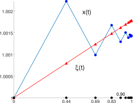
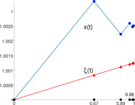
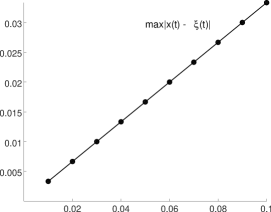
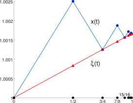
It seems to be impossible to find a precise analytical estimate of difference $\left|x(t)-\xi(t)\right|$ in terms of $\varepsilon$. Instead we conducted numerical modelling and found empirical dependence between proximity of solutions and small parameter $\varepsilon$. The results of modelling are presented in Figure 1.

a) Solutions of original and averaged systems, $\varepsilon=0.005$, $q=2$

a) Solutions of original and averaged systems, $\varepsilon=0.005$, $q=1.8$

a) Solutions of original and averaged systems, $\varepsilon=0.005$, $q=3$

d) Absolute difference between solutons in regard to $\varepsilon$

Figure 1. Numerical modelling of averaging method for quasiperiodic system on time scale $\mathbb{T}=\left\{t_{n}=1-\dfrac{1}{q^{n}},n\in\mathbb{N}_{0},q>1\right\}\cup\left\{1\right\}$.

4. Conclusion.

The aim of this paper is to develop our previous results for the averaging method on time scales. Following [Adivar(2013)] we considered $\Delta$–periodic systems and obtained a more accurate estimate for proximity between solutions of original and averaged systems. Moreover, the same result was obtained for dynamic systems with a quasiperiodic right-hand side, which are introduced for the first time. To illustrate the application of the averaging theorem for such kind of system we considered an example and conducted numerical modelling. Obtained results can be used to improve previously developed numerically–asymptotic method of solution for optimal control problems on time scales.

References

• [Adivar(2013)] Adivar, M., 2013. A new periodicity concept for time scales. Mathematica Slovaca , 817–828.
• [Bogolyubov and Mitropol’skii(1961)] Bogolyubov, N.N., Mitropol’skii, Y.A., 1961. Asymptotic Methods in the Theory of Nonlinear Oscillations. Gordon & Breach, Delhi.
• [Bohner and Peterson(2002)] Bohner, M., Peterson, A., 2002. Advances in Dynamic Equations on Time Scales. Springer Science & Business Media.
• [Bohner and Peterson(2012)] Bohner, M., Peterson, A., 2012. Dynamic equations on time scales: An introduction with applications. Springer Science & Business Media.
• [Hilger(1988)] Hilger, S., 1988. Ein Maßkettenkalkül mit Anwendung auf Zentrumsmannigfaltigkeiten. Ph.D. thesis. Universität Würzburg.
• [Kichmarenko and Ogulenko(2017)] Kichmarenko, O.D., Ogulenko, A.P., 2017. Averaging of multicriteria control problems of systems on time scales. Journal of Computer and Systems Sciences International 56, 33–43.
• [Krylov and Bogolyubov(1947)] Krylov, N.M., Bogolyubov, N.N., 1947. Introduction to Nonlinear Mechanics. Princeton Univ. Press, Princeton.
• [Ogulenko(2017)] Ogulenko, A.P., 2017. Partial averaging of the systems on time scales. Researches in mathematics and mechanics 22, 32–45.
• [Ogulenko and Kichmarenko(2012)] Ogulenko, A.P., Kichmarenko, O.D., 2012. A scheme of full averaging on time scales. Visn. Odes. Nat. Univ. Mat. Mekh. 17, 67–77. In Russian.
• [Ogulenko and Kichmarenko(2016)] Ogulenko, A.P., Kichmarenko, O.D., 2016. Averaging of the problem of optimal control on time scales. Journal of Mathematical Sciences 212, 290–304.
• [Plotnikov(1992)] Plotnikov, V.A., 1992. Method of Averaging in the Problems of Control. Lybid’, Kiev, Odessa. In Russian.
• [Slavík(2012)] Slavík, A., 2012. Averaging dynamic equations on time scales. Journal of Mathematical Analysis and Applications 388, 996–1012.