Coupling Finite Element Method with Large Scale Atomic/Molecular Massively Parallel Simulator (LAMMPS)
for Hierarchical Multiscale Simulations

Abstract

In this work, we have developed a multiscale computational algorithm to couple finite element method with an open source molecular dynamics code — the Large scale Atomic/Molecular Massively Parallel Simulator (LAMMPS) — to perform hierarchical multiscale simulations in highly scalable parallel computations. The algorithm was firstly verified by performing simulations of single crystal copper deformation, and a good agreement with the well-established method was confirmed. Then, we applied the multiscale method to simulate mechanical responses of a polymeric material composed of multi-million fine scale atoms inside the representative unit cells (r-cell) against uniaxial loading. It was observed that the method can successfully capture plastic deformation in the polymer at macroscale, and reproduces the double yield points typical in polymeric materials, strain localization and necking deformation after the second yield point. In addition, parallel scalability of the multiscale algorithm was examined up to around 100 thousand processors with 10 million particles, and an almost ideal strong scaling was achieved thanks to LAMMPS parallel architecture.

1 Introduction

Multiscale simulation methods, which couple atomistic models with continuum models, are advanced computational technologies aimed to understand material properties under specific conditions without using any empirical or experimental information. The multiscale approach is not simply a computational convenience, but deeply rooted in material physics, because almost all physical events in nature are inherently multiscale phenomena with different time and length scales. In past two decades, a variety of multiscale techniques have been proposed and developed e.g. tadmor2011 ; liu2004 ; To2005 ; Murashima2013 . In general, the multiscale methods in condensed matters may be categorized into two major classes; the concurrent multiscale modeling and the hierarchical multiscale modeling.

The concurrent multiscale approach directly connects continuum and atomistic models by communicating displacement or force of atoms to nodes, particles or quadrature points of continuum body on-the-fly to link microscale and macroscale. Since the latter half of the 1990s, several pioneering multiscale methods on coupling atomistic methods with finite elements have extensively studied. Broughton et al. have conducted fracture simulation of Silicon by coupling finite element method (FEM), molecular dynamics (MD) simulation, and tight binding quantum calculation though a handshake Hamiltonian abraham1998 ; broughton1999 . The bridging scale method uses a projection operator to decompose the total displacement field into mutually orthogonal coarse and fine scales, leading to a coupled multiscale equations of motion in the MD and FEM models respectively, e.g. wagner2003 ; xiao2004 . Recently, Li and his co-workers have proposed a novel decomposition method of MD simulation, namely multiscale micromorphic molecular dynamics (MMMD), to model transition zone between microscale and macroscale thorough mesoscale region li2016 . The method allows us to couple MD simulations and FEM urata2016 or Peridynamics tong2016 , which usually models nonlocal continuum media by using particle discretization.

The other category of multiscale modelings is hierarchical coupling method, which locally embeds fine scale models into coarse scale models. A conventional procedure to build a hierarchical modeling is adopting micromechanics homogenization approach by employing a so-called representative volume elements (RVE) e.g. sheng2004 ; valavala2009 ; wernik2014 . One of the most successful hierarchical multiscale approaches is the quasicontinuum (QC) method proposed by Tadmore et al., in which the finite element mesh covers the entire simulation system, and the mesh may be scaled-down to atomic dimensions at selected locations, in which the fine scale modeling is in terms of molecular statics or energy minimization or optimization tadmor1996 ; tadmor1999 ; miller2002 . A similar but much simpler hierarchical approach is the so-called Cauchy-Born rule (CBR) method, which assumes affine deformation in crystal lattice, and it thus allows us to couple atomistic and continuum models directly through constant deformation gradient and direct bottom-up upscale. Thus, CBR was in principle only applicable to crystalline materials, because it is based on the assumption of uniform deformation of crystal lattices; however, the idea has been further extended to nonuniform deformation in crystalline solids by considering higher order deformation gradients e.g. sunyk2003 ; weinan2007 . For instance, the higher order CBR has been combined with crystal defect dynamics lyu2017 ; lyu2019 and cohesive zone model urata2017a to investigate more complicated dislocation pattern dynamics and fracture mechanics of crystals.

Recently, the present authors have extended the idea of the lattice statics-based Cauchy-Born rule to amorphous solids to conduct hierarchical multiscale modeling of inelastic deformation in an amorphous solid urata2018 . The method was called as the coarse-grained (CG) Parrinello-Rahman (PR) method, since the molecular statics in the representative unit cell of the fine scale model is used analogous to that of PR-MD simulation parrinello1980 . The CG-PR method was systematically validated by comparing its numerical simulation results with that of MD simulations, and the CG-PR method was applied to study the mechanical responses of a Lennard-Jones (LJ) binary glass and amorphous silica models urata2017b . It has been shown that the CG-PR method can successfully reproduce shear band formation in a single-notched amorphous solids using relatively coarse mesh FEM models at macroscale urata2018 . The advantage of CG-PR method is its independence of the constitutive empiricism, or in other words, it does not need any ad hoc empirical modelings of complicated constitutive relation of amorphous solids. However, a critical drawback of the method is its expensive computation cost, because a representative unit cell (r-cell) composed of many atoms is needed for each and every quadrature points of a FEM model, thus it requires running an enormous number of atomistic simulations all together at the same time. Thus, it calls an effective parallel computation algorithm for the proposed multiscale method, which is crucial for any practical application of such method.

In this work, to improve computational efficiency of our in-house CG-PR code, the CG-PR algorithm was coupled with the large scale parallel MD code, namely the large scale atomic/molecular massively parallel simulator (LAMMPS) plimpton1995 ; LAMMPS . To do so, we first develop a coupling algorithm for a single MD cell, whose shape is represented by an upper triangular stretch matrix of six components, instead of general non-symmetric r-cell mentioned in section 2. In section 3, we first discuss the validation of the multiscale algorithm and multiscale code, which were first validated by performing a numerical simulation of deformation of crystalline copper. Then, we conducted a large-scale parallel computation for simulation of inelastic deformation of a polymeric material to demonstrate applicability of the method, which is implemented in a massively parallel supercomputer. Finally, in Section 4, we summarize and conclude the work.

2 Computational Methods

We first discuss coupling between molecular dynamics (MD) with finite element method (FEM).

2.1 Coupling MD and FEM

To start, we first prepare a representative unit cell (r-cell) whose shape is represented by a second order tensor or a matrix ${\bf H}$. Atom position in the r-cell can be represented by a scaled atom position vector (${\bf S}_{i}(t)$) for atom $i$, and then the current position of the atom $i$ at time $t$ can be written as,

$${\bf r}_{i}(t)={\bf H}(t)\cdot{\bf S}_{i}(t).$$ (1)

Employing CBR, we couple the deformation of an r-cell within an element in a continuum model, we may express the cell shape tensor as,

$${\bf H}_{e}(t)={\bf F}_{e}(t)\cdot{\bf H}_{e}(0),$$ (2)

where ${\bf F}_{e}$ is deformation gradient tensor of an element $e$, and ${\bf H}_{e}(0)$ is an initial shape of the r-cell. Thus, the current position of an atom in an r-cell of the given $e$-th element is expressed as,

$${\bf r}_{i}^{e}(t)={\bf H}_{e}(t)\cdot{\bf S}_{i}(0)={\bf F}_{e}(t)\cdot{\bf H}_{e}(0)\cdot{\bf S}_{i}(0).$$ (3)

To apply a general MD code for hierarchical multiscale modeling, the shape tensor ${\bf H}_{e}(t)$ should correspond to shape of an MD unit cell. However, the shape tensor ${\bf H}_{e}(t)$ is not symmetric and composed of independent nine components, while MD unit cell in LAMMPS should be upper triangular matrix with six components. The shape tensor can be decomposed to a stretch tensor and a rotation tensor. The stretch tensor, represented by the upper triangular matrix, satisfies the periodic boundary conditions of the initial orthogonal basis, whereas the rotation tensor violates the periodic boundary conditions. We need to treat the stretch tensor and the rotation tensor separately to implement the general purpose MD code to the multiscale simulation in the following way.

In our algorithm, we therefore decompose the deformation gradient tensor ${\bf F}_{e}$ into an orthogonal rotation matrix ${\bf Q}_{e}$ and an upper triangular stretch matrix ${\bf R}_{e}$ as follows.

$${\bf F}_{e}(t)={\bf Q}_{e}(t)\cdot{\bf R}_{e}(t).$$ (4)

This process is conventional QR decomposition, which is calculated by the Gram-Schmidt orthogonalization. Note that the triangular stretch matrix ${\bf R}$ should be positive definite. Otherwise, the stretch matrix ${\bf R}$ will introduce wrong axial inversion.

Instead of directly using ${\bf F}_{e}(t)$, the upper triangular stretch matrix ${\bf R}_{e}$ can be used as a deformation matrix of the MD unit cell as,

$${\bf H}_{\rm MD}(t)={\bf R}_{e}(t)\cdot{\bf H}_{e}(0),$$ (5)

where ${\bf H}_{\rm MD}(t)$ represents shape of the MD unit cell at time $t$. It is therefore, in a MD code, atomic coordinate should be

$${\bf r}_{i}^{\rm MD}(t)={\bf R}_{e}(t)\cdot{\bf H}_{e}(0)\cdot{\bf S}_{i}(0).$$ (6)

Once we know the current atom coordinate, ${\bf r}_{i}^{\rm MD}(t)$, a MD code can calculate the stress of the MD unit cell ($\bm{\sigma}_{\rm MD}(t)$) using an interatomic interaction potential. The stress in MD coordinate system is transferred to the real coordinate system of FEM by using the rotation matrix ${\bf Q}_{e}$ as follows,

$$\bm{\sigma}_{\rm FEM}(t)={\bf Q}_{e}(t)\cdot\bm{\sigma}_{\rm MD}(t)\cdot{\bf Q}_{e}^{T}(t).$$ (7)

In FEM code, the first Piola-Kirchhoff stress is used to evaluate a force acting on each node.

$${\bf P}_{\rm FEM}(t)=J\bm{\sigma}_{\rm FEM}(t)\cdot{\bf F}_{e}^{-T}(t),$$ (8)

where $J$ is the Jacobian of the deformation gradient tensor ${\bf F}$.

In our multiscale code, we used LAMMPS as the MD calculation engine. Because LAMMPS memorizes previous deformation matrix, ${\bf R}(t-1)$, our FEM code provides the following differentiation between current and previous upper triangular stretch matrices to LAMMPS.

$$\Delta{\bf R}_{e}(t)={\bf R}_{e}(t)\cdot{\bf R}_{e}^{-1}(t-1).$$ (9)

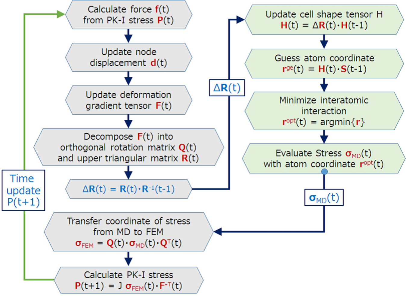
The flow chart of the proposed multiscale computation algorithm is schematically depicted in Fig. 1, and its validity will be examined in Sec. 3.1.

Figure 1: Flowchart of the multiscale computation algorithm that couples a continuum finite element simulation with a general MD simulation code.

2.2 Hierarchical coupling method for amorphous polymers

Here we briefly introduce the algorithm of CG-PR method, which has been developed as a hierarchical multiscale modeling tool for amorphous solids (see urata2018 ; urata2017b ).

In the framework of finite element method, the discrete equations of motion for nodal displacements can be evaluated form the following equation,

$$\mathbf{M}\cdot\ddot{\mathbf{d}}+\mathbf{f}^{\rm int}(\mathbf{d})=\mathbf{f}^{\rm ext},$$ (10)

where $\mathbf{d}$ is node displacement vector, and $\mathbf{M}$, $\mathbf{f}^{\rm int}$, and $\mathbf{f}^{\rm ext}$ are the mass matrix, force vectors, and external force, respectively. These quantities are defined as follows,

$$\mathbf{M}=\mathop{\bf A}\limits_{e=1}^{n^{e}}\int_{\Omega_{e}}\rho_{0}\mathbf{N}_{e}^{T}\cdot\mathbf{N}_{e}dV,$$ (11)

$$\mathbf{f}^{\rm int}=\mathop{\bf A}\limits_{e=1}^{n^{e}}\int_{\Omega_{e}}\mathbf{B}_{e}^{T}\cdot\mathbf{P}_{e}({\bf d})dV,$$ (12)

$$\mathbf{f}^{\rm ext}=\mathop{\bf A}\limits_{e=1}^{n^{e}}\Bigr{\{}\int_{\Omega_{e}}\mathbf{N}_{e}^{T}\cdot\mathbf{B}_{e}dV+\int_{\partial\Gamma_{t}}\mathbf{N}_{e}^{T}\cdot\bar{\mathbf{T}}_{e}dS\Bigl{\}},$$ (13)

where, $\mathop{\bf A}\limits$ is the element assemble operator acting over all elements; $\rho_{0}$ is the material density; $\mathbf{N}_{e}$ is the element shape function matrix; $\bar{\mathbf{T}}_{e}$ is the traction vector on the surface, and $\mathbf{B}_{e}$ is the element strain-displacement matrix as,

$$\mathbf{B}_{e}:=\Biggl{[}\frac{\partial\mathbf{N}_{e}}{\partial X}\Biggr{]}~{}.$$ (14)

In Eq. (12), $\mathbf{P}_{e}$ is the first Piola-Kirchhoff stress, which can be evaluated using interatomic interaction among atoms in an r-cell as follows,

$${\bf P}={1\over 2\Omega_{0}}{\partial W\over\partial{\bf F}}={1\over 2\Omega_{0}}\sum_{i,j}{\partial V(r_{ij})\over\partial r_{ij}}{{\bf r}_{ij}\otimes{\bf R}_{ij}\over r_{ij}}~{},$$ (15)

where ${\bf R}_{ij}={\bf H}(0)\cdot{\bf S}_{ij}$ is the relative position vector between initial positions of atoms $i$ and $j$, and ${\bf r}_{ij}={\bf r}_{j}-{\bf r}_{i}$ is the position vector between current positions of atoms $i$ and $j$. $V$ is interatomic potential as a function of distance $r_{ij}$ and $\Omega_{0}$ is the volume of r-cell. In the case of single crystal, atom position ${\bf r}$ is unique, but this is not the case for amorphous solids. Optimizing the potential energy respect to distance $r$, we can obtain the optimized position vector ${\bf r}_{i}^{\rm opt}$ as,

$${\bf r}_{i}^{\rm opt}(t)={\rm argmin}{V({\bf r}_{i}^{\rm ge})}~{},$$ (16)

where ${\rm argmin}$ stands for argument of the minimum, ${\bf r}^{\rm ge}_{i}(t)$ is the position guessed from previous configuration at time $t-1$,

$${\bf r}^{\rm ge}_{i}(t) = {\bf F}(t)_{e}\cdot{\bf H(0)}_{e}\cdot{\bf S}_{i}(t-1).$$ (17)

This equation is essentially based on the Cauchy-Born rule, because the guessed atom coordinates are uniformly determined following the deformation gradient in an element.

Once we have found ${\bf r}_{i}^{\rm opt}$, the following coordinates can be obtained.

$${\bf S}^{\rm opt}_{i} = ({\bf F}(t)_{e}\cdot{\bf H(0)}_{e})^{-1}\cdot{\bf r}^{\rm opt}_{i},$$ (18)

$${\bf R}^{\rm opt}_{i} = {\bf H(0)}_{e}\cdot{\bf S}_{i}^{\rm opt}.$$ (19)

Then, the correct 1st Piola-Kirchhoff stress is eventually defined as follows,

$${\bf P}={1\over 2\Omega_{0}}{\partial W\over\partial{\bf F}}={1\over 2\Omega_{0}}\sum_{i,j}{\partial V(r^{\rm opt}_{ij})\over\partial r^{\rm opt}_{ij}}{{\bf r}^{\rm opt}_{ij}\otimes{\bf R}^{\rm opt}_{ij}\over r^{\rm opt}_{ij}}~{}.$$ (20)

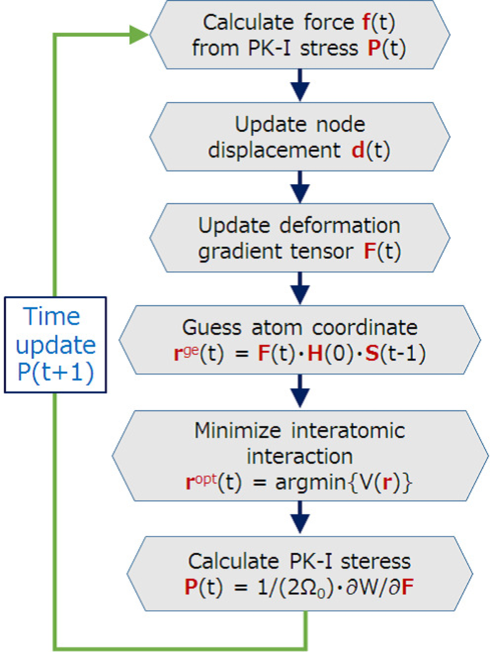
If we use a general MD code, the 1st Piola-Kirchhoff stress is calculated using Eq.(8) with the optimized coordinate ${\bf r}^{\rm opt}$. The flowchart of the above algorithm is shown in Fig. 2.

Figure 2: Flowchart of the Coarse-grained Parrinello-Rahman (CG-PR) method. urata2018 ; urata2017b

2.3 Implementation of parallel MD systems in LAMMPS

In the proposed multiscale model, each element at continuum FEM scale has its own MD system, i.e. fine scale r-cells at every FEM quadrature points. LAMMPS can divide the MD system into multiple systems so that these systems are independent from others by splitting a message passing interface (MPI) communicator to multiple communicators assigned to each MD systems. These MD systems are independent at the MD simulation level, while exchanging the energy and momentum among them through FEM. Since the size of FEM is small in the present work, FEM is computed on a parent node, and LAMMPS is computed on full nodes. To communicate FEM and LAMMPS, simple scatter and gather algorithm has been implemented. The cost of the MPI communication is very small, and we shall discussed it in Sec. 3.2.

3 Results

3.1 Model validation

Figure 3: Deformation patterns used for validation tests. “t” and “c” represent tensile and compress.

Figure 4: Comparison of stresses evaluated using two algorithms for simple deformation (Fig. 3 (A)). One is coupling method with a general MD code using Eqs.(1)–(9), and the other one is original in-house code with Eqs.(16)–(20).

First of all, to test our multiscale code that couples the open-source MD code LAMMPS with FEM method, we compare the stresses evaluated by the two independent algorithms mentioned above, i.e. the one that uses Eqs.(16)–(20) and the other one that uses LAMMPS with Eqs.(1)–(9). A crystalline copper model, which is composed of $10\times 10\times 10$ FCC primitive cells, is used for the validation test. The supercell includes 4,000 atoms and the side length is 36.15 Å. Mishin’s EAM potential mishin2001 was employed to evaluate interatomic interaction.

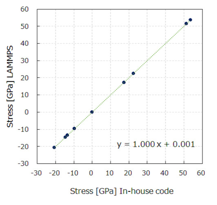
Uniaxial stretching/compression and two kinds of asymmetric deformations were examined as schematically illustrated in Fig. 3. In the first case, the unit cell was simply elongated and compressed along z-axis with maintaining the cell length of the other two sides. The stresses in every components evaluated using two methods are compared in a scatter diagram in Fig. 4, confirms that the stresses calculated by the two codes agree well for the symmetric deformation.

Next, we examined how the multiscale algorithm works when it is applied to simulate asymmetric deformations, in order to verify the multiscale algorithm ability to use QR decomposition to couple with a MD engine, which is LAMMPS in this case. In Case (B), one edge is displaced from -0.3 to +0.3 strain along $y$-axis, whereas the edge is moved within the same range of strain for the [111]-direction at the same time in the case of Case (C). In Table 1, we summarize the deformation gradient tensor ${\bf F}$, the orthogonal rotation tensor ${\bf Q}$, and the upper triangular stretch tensor ${\bf R}$ in addition to all stress components in both coordinate systems of LAMMPS and FEM. One may find that all stresses calculated by using QR decomposition (Eqs.(1)–(9).), $\bm{\sigma}_{\rm FEM}$, agree to those of the in-house CG-PR code with Eqs.(16)–(20), $\bm{\sigma}_{\rm IH}$. It is therefore reasonable to expect that the proposed multiscale coupling algorithm may be able to simulate even more complicated asymmetric deformations, which may not be feasible to simulate by using the Parrinello-Rahman method parrinello1980 with the periodic boundary conditions.

In the next section, we shall demonstrate a large scale multiscale simulation of inelastic deformation of a polymeric material.

Table 1: Comparison of stresses [GPa] evaluated using in-house code $\bm{\sigma}_{\rm IH}$ and the coupling method with LAMMPS $\bm{\sigma}_{\rm FEM}$ for deformation drawn in Fig. 3 (B) and (C). In Case (B), one edge is displaced with 0.3 or -0.3 strain along $Y$-axis. In Case (C), one edge is moved in 0.3 or -0.3 strain along the [111]-direction. (t) and (c) stand tensile and compressive loadings, respectively. Deformation gradient tensor F and the decomposition to the orthogonal rotation matrix ${\bf Q}$ and the upper triangular stretch matrix ${\bf R}$ are also displayed. The last line shows the $L2$-norm (spectral norm) of the error between $\bm{\sigma}_{\rm IH}$ and $\bm{\sigma}_{\rm FEM}$.

Fig. 3	B(t)			B(c)			C(t)			C(c)
	1.000	0.000	0.000	1.000	0.000	0.000	1.075	0.075	0.075	0.925	-0.075	-0.075
F	-0.075	1.075	0.075	0.075	0.925	-0.075	0.075	1.075	0.075	-0.075	0.925	-0.075
	0.000	0.000	1.000	0.000	0.000	1.000	0.075	0.075	1.075	-0.075	-0.075	0.925
	0.997	0.075	0.000	0.997	-0.075	0.000	0.995	-0.074	-0.065	0.993	0.073	0.088
Q	-0.075	0.997	0.000	0.075	0.997	0.000	0.069	0.995	-0.065	-0.081	0.993	0.088
	0.000	0.000	1.000	0.000	0.000	1.000	0.069	0.060	0.996	-0.081	-0.094	0.992
	1.003	-0.080	-0.006	1.003	0.069	-0.006	1.080	0.154	0.154	0.931	-0.143	-0.143
R	0.000	1.072	0.075	0.000	0.922	-0.075	0.000	1.069	0.134	0.000	0.920	-0.167
	0.000	0.000	1.000	0.000	0.000	1.000	0.000	0.000	1.061	0.000	0.000	0.905
	-7.536	3.844	0.731	12.786	-8.959	1.312	-15.403	-5.232	-4.614	75.792	17.495	21.018
$\bm{\sigma}_{\rm MD}$	3.844	-9.429	-3.615	-8.959	18.757	9.232	-5.232	-13.891	-3.995	17.495	81.230	24.536
	0.731	-3.615	-6.974	1.312	9.232	14.155	-4.614	-3.995	-12.884	21.018	24.536	90.283
	-6.974	3.660	0.458	14.155	-9.304	0.618	-14.060	-4.698	-4.698	82.435	21.629	21.629
$\bm{\sigma}_{\rm FEM}$	3.660	-9.992	-3.660	-9.304	17.387	9.304	-4.698	-14.060	-4.698	21.629	82.435	21.629
	0.458	-3.660	-6.974	0.618	9.304	14.155	-4.698	-4.698	-14.060	21.629	21.629	82.435
	-6.975	3.660	0.458	14.154	-9.304	0.618	-14.061	-4.698	-4.698	82.433	21.629	21.629
$\bm{\sigma}_{\rm IH}$	3.660	-9.993	-3.660	-9.304	17.386	9.304	-4.698	-14.061	-4.698	21.629	82.433	21.629
	0.458	-3.660	-6.975	0.618	9.304	14.154	-4.698	-4.698	-14.061	21.629	21.629	82.433
$||\Delta\bm{\sigma}||_{2}$		0.001			0.001			0.001			0.002

3.2 Large-scale parallel multiscale computation for polymer deformation

In this section, we report the results of using the coupled FEM-LAMMPS code to investigate inelastic deformation of a macroscale cubic polymeric specimen composed of many mono-disperse linear polymers. A schematic illustration of the numerical model is shown in Fig. 5. The coarse-grained polymer model, namely, the bead-spring model KremerGrest1990 , was used to describe the polymer chains in r-cells. The polymer chain is composed of LJ particles linearly connected by finite extensively nonlinear elastic bonds. The potential parameters were set to the standard Kremer-Grest model KremerGrest1990 . The cubic specimen is composed of $100$ tetrahedron finite elements, and each element has an r-cell that contains $100$ polymer chains, and each of them is composed of $100$ beads. In FEM calculation, each quadrature point is represented by an r-cell. Because of the linear four-node tetrahedron element is used in FEM modeling, each element has only one quadrature point. Thus, the total number of beads in fine scale model of the system is $100\times 100\times 100=10^{6}$, i.e. one million atomistic freedoms. Initial states of polymers were prepared by using OCTA-COGNAC OCTA-COGNAC , where the polymers were equilibrated in melt condition. To impose the uniaxial stretch boundary condition to the polymeric material, the constant velocities were prescribed at both top and bottom surfaces of the cubic specimen along vertical direction. The sides of the material were free to move. The magnitude of the prescribed velocity was chosen sufficiently large so that one can observe nonlinear behaviors of the polymeric material. When the deformation rate is higher than a characteristic value $1/\tau_{\rm R}$, where $\tau_{\rm R}$ is the Rouse relaxation time of polymer chains, the polymeric material is expected to show a nonlinear behavior in an extensional deformation Murashima2018 . In the case of polymer melt with 100 beads per a chain, $\tau_{\rm R}\simeq 10,000[\tau]$, where $\tau$ is the unit of time of LJ particle. The results are summarized in Fig. 6.

Figure 5: Schematic illustration of multiscale simulation for a polymeric material: a cubic material with finite element mesh (a) and polymers in a r-cell (b).

Figure 6: The tensile stress versus the tensile strain of uniaxially stretched polymeric material obtained from the multiscale simulation (a). The unit of the stress here is $[\epsilon/\sigma^{3}]$, $\epsilon$ and $\sigma$ are the unit of energy and the unit of size of LJ particle in a coarse-grained polymer, respectively. Molecular dynamics simulation results under different uniaxial engineering strain rates (0.01, 0.015, 0.020 $[1/\tau]$) are also shown in Fig (a). Inset in Fig (a) focuses on the transition from elastic to plastic deformation. Figures (b) to (f) represent the appearances of the material during deformation at characteristic strain found in Fig. (a). The color shown in Figs. (b) to (f) represents the magnitude of the stress at the local finite element; blue is low and red is high.

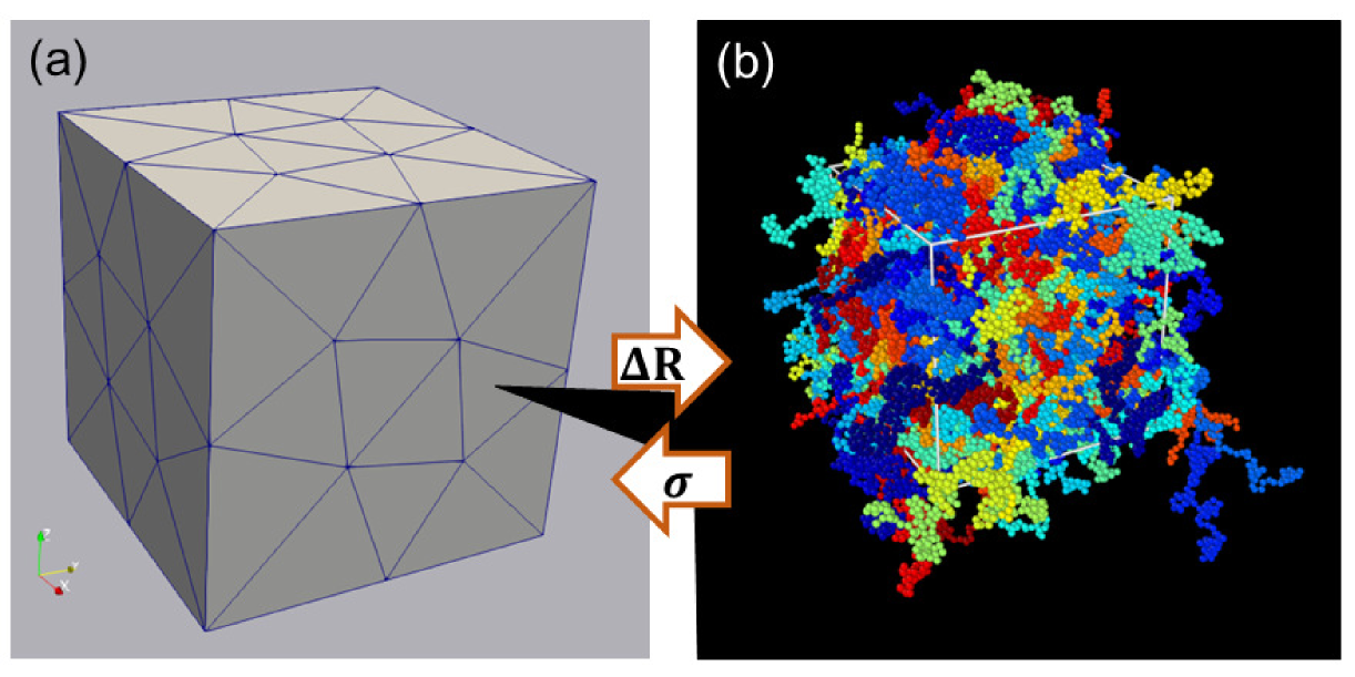
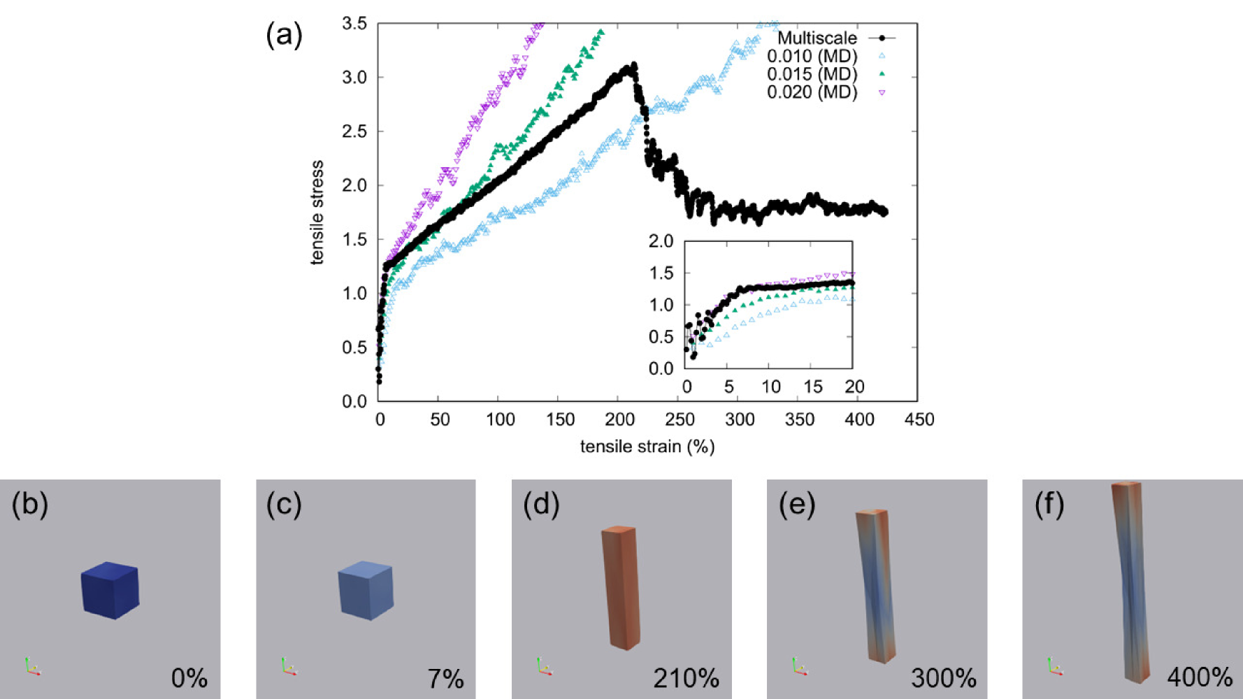
Figure 6(a) shows the tensile stress versus the tensile strain, where the tensile stress defined here is the magnitude of the largest eigenvalue of the stress tensor $\bm{\sigma}_{\rm FEM}$ averaged over the whole system. The tensile strain was estimated from the uniaxial engineering strain rate $2.0\times 10^{-5}$ [1/FEM step] multiplied by the FEM steps. The unit of the stress is [$\epsilon/\sigma^{3}$], where $\epsilon$ and $\sigma$ are the units of the energy and the length of LJ coarse-grained polymer chain, respectively. For comparison, we carried out the molecular dynamics simulation of the Kremer-Grest model on the periodic boundary conditions, namely the unit cell of the multiscale simulation. We applied uniaxial engineering strain rates ($0.01,0.015,0.02[1/\tau]$) to the system at $T=0.1$ which was selected since the temperature dependence of the stress-strain curve is negligible when the temperature is less than the glass transition temperature 0.35 Bennenman1998 . The results of the molecular dynamics simulation were also shown in Fig. 6(a). Figures 6(b) to (f) show the appearances of the material at the characteristic tensile strain; 0% (initial state, b), 7% (first yield point, c), 210% (second yield point, d), 300% (lower yield point, e), 400% (final state, f). The double yield points observed in polymeric materials have been investigated and the second yield point relates to the necking phenomena Brooks1992 . The tensile stress increases monotonically from (b) to (c) and from (c) to (d). The first yield point (c) is the onset of the plastic deformation. The former region is the elastic deformation region and the latter region is the plastic deformation region. The shape of the material is a rectangular parallelepiped in these small strain regions. Beyond the second yield point (d), the tensile stress decreases and the material show necking. The first yield point appeared around the 7% strain both in the multiscale simulation and the molecular dynamics simulation with the periodic boundary conditions. When the strain is higher than the first yield point, the stress-strain curves show different slopes owing to its strain-rate dependence. The molecular dynamics simulation did not show the second yield point that is around the strain 200%. The reason for the difference between the multiscale simulation and the molecular dynamics simulation is that the molecular dynamics simulation was carried out under periodic boundary condition without the free-surfaces, which prevents necking. However, even if the large scale molecular dynamics simulation with the surfaces were carried out, the necking behavior was not observed in the amorphous polymeric material Yashiro2003 . On the other hand, the coarse-grained molecular dynamics simulation of polyethylene lamellar structures, consisting of crystalline and amorphous layers, has shown a necking like behavior, where a neck is formed in the weak amorphous layers and propagates down in the specimen  Higuchi2017 . It is believed that inhomogeneity may play a key role in formation of necking in amorphous polymeric materials. Capturing necking formation in the amorphous polymer in the molecular dynamics simulation is still a challenging problem. The present multiscale solution, however, has somewhat overcome this difficulty in the large scale hierarchical multiscale simulation.

The material behaviors observed from Fig. 6 are qualitatively consistent with the experimental observation from an uniaxially melt-extruded high-density polyethylene films, e.g. ZhouWilkes1998 . The second yield point has been observed when the engineering strain is about 200% both in our simulation and in the experiment reported. Nevertheless, the initial condition of the polymer specimen in the simulation was in amorphous state while that in the experiment was crystalline lamellae. It was also speculated that the yield point may depend on the sample size and the direction of stretch (see ZhouWilkes1998 ). Further investigation, adjusting the conditions between the simulation and the experiment, is still ongoing.

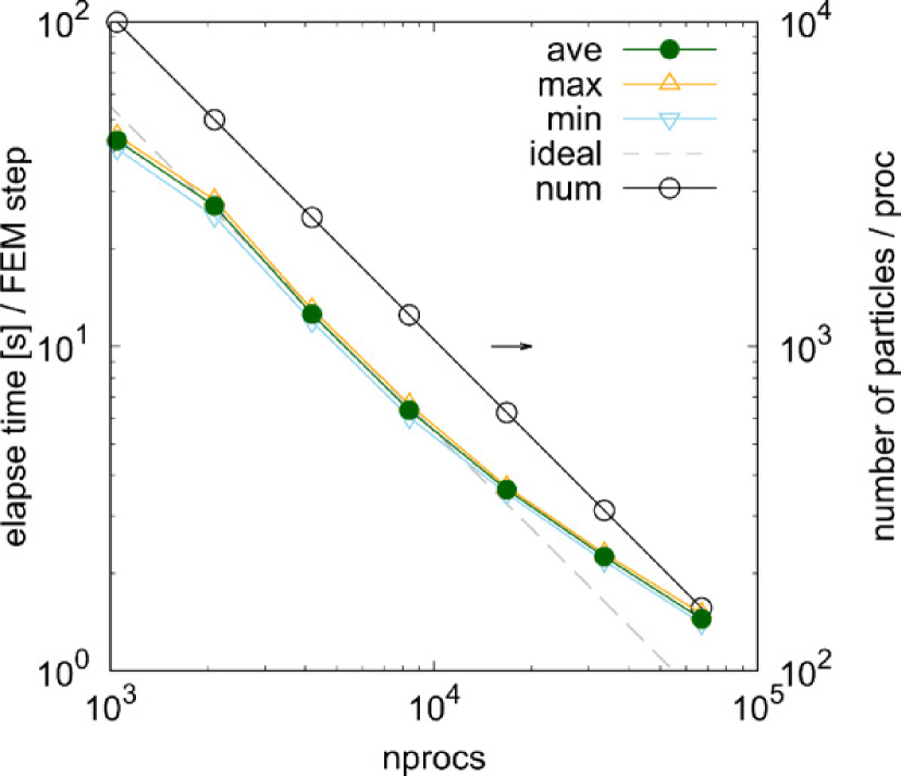
Moreover, we have studied parallel scalability of our multiscale code on K computer Knotes . In the study, the total number of elements in the FEM model is up to one thousand, and the total number of particles in a system is up to 10 millions. Elapsed CPU time [unit s] per a multiscale FEM time step was measured and averaged over 10 FEM steps, which includes the iteration time for running the fine scale CG-PR method in each r-cell. As maybe found in Fig. 7, our multiscale simulation result shows a nearly ideal scaling efficiency when the number of particles per a processor is larger than 100. Generally speaking, parallel scalability of a direct MD simulation with 10 million particles saturates when the number of processors reaches to 10 thousands. The reason for the high scaling efficiency of the hybrid method implemented with FEM and LAMMPS may be attributed to the facts that (1) the multiscale method, especially the natural segregated distribution of r-cells, makes efficient use of the massively parallel architecture of the supercomputer used such as K computer, and (2) the CG-PR molecular statics minimization algorithm may have less or no computing overhead.

Figure 7: Parallel scaling of multiscale simulation on K computer. The simulation system was composed of one thousand finite elements and each finite element had 10 thousand LJ particles (100 bead-spring chains with 100 beads). The items, “ave”, “max” and “min”, are the average, maximum, and minimum times (left vertical axis) in 10 multiscale FEM steps, respectively, “ideal” is the ideal parallel scaling line for guide to eyes, and “num” is the number of particles per a processor (right vertical axis). Note that each MD simulation in the multiscale simulation is not parallelized when the number of processors is $10^{3}$.

4 Conclusions

In this work, we have developed a hierarchical multiscale method to bridge finite element method with molecular dynamics by using the large scale atomic /molecular massively parallel simulator (LAMMPS). In the developed computation algorithm, a QR decomposition is used and implemented to couple deformations with stresses at both FEM level as well as MD level, and in between. The multiscale coupling algorithm was validated by applying typical deformation patterns on Copper crystal model, and a good agreement between MD simulation results with the results obtained from the CG-PR method is confirmed.

We have applied the multiscale code simulating uniaxial deformation of a polymeric material in a multiscale CG-PR/FEM model that is composed of one million fine scale r-cell of Lennard-Jones particles, and we have succeeded in observing nonlinear elastic-plastic deformation behavior of amorphous polymeric materials, including strain localization (almost necking) in the polymeric material. Indeed, a yield point has appeared when the tensile strain is about 200%, which is consistent with the experimental observation.

It is worthy noting that the four-node tetrahedral element (C3D4) has a relative lower interpolation order, and it is often too stiff to be used in inelastic finite deformation computations. The inelastic deformation simulation results reported in this work by using C3D4 element is remarkable, which could not be achieved by using the same type of element in the phenomenological computational plasticity. In the proposed multiscale computational algorithm, the r-cell at each Gauss point can change the volume in accordance with the stress field through the hierarchical coupling. The comparability of the r-cell may avoid the locking issue caused in the usual FEM model.

In addition, we also examined parallel scalability of the multiscale code using a large FEM model, in which ten million fine scale particles are embedded. The result revealed that the code has a strong, nearly ideal, scaling ability up to ten thousand processors thanks to the highly efficient built-in scalability of LAMMPS. The large scale simulations reported in this paper demonstrated applicability of the multiscale coupling method and algorithm to model and simulate mechanical properties of amorphous materials.

Authors’ contributions

TM designed the concurrent coupling algorithm and developed a code to establish interface with LAMMPS. SU developed the multiscale simulation code coupling FEM and LAMMPS, and performed validation tests. TM conducted large scale simulation for the polymeric material. TM and SU wrote simulation parts of the manuscript, and SL supervised the project, wrote and summarized the manuscript. All the authors have read and approved the final manuscript.