Quickly Inserting Pegs into Uncertain Holes using Multi-view Images and Deep Network Trained on Synthetic Data

Abstract

This paper uses robots to assemble pegs into holes on surfaces with different colors and textures. It especially targets at the problem of peg-in-hole assembly with initial position uncertainty. Two in-hand cameras and a force-torque sensor are used to account for the position uncertainty. A program sequence comprising learning-based visual servoing, spiral search, and impedance control is implemented to perform the peg-in-hole task with feedback from the above sensors. Contributions are mainly made in the learning-based visual servoing of the sequence, where a deep neural network is trained with various sets of synthetic data generated using the concept of domain randomization to predict where a hole is. In the experiments and analysis section, the network is analyzed and compared, and a real-world robotic system to insert pegs to holes using the proposed method is implemented. The results show that the implemented peg-in-hole assembly system can perform successful peg-in-hole insertions on surfaces with various colors and textures. It can generally speed up the entire peg-in-hole process.

I Introduction

One goal in robotics is to automate product assembly. At present, most robotic assembly systems, such as the ones implemented in the production of cars, still follow the basic principle of teaching and playback. The teaching and playback concept is useful when the target objects are fixed. When variations exist, the usefulness of teaching and playback principle is limited. This leads people to use automatic motion planning to assemble a diverse range of products with variations.

An important issue of automatic motion planning is the accumulated position errors. The goal pose after execution could be very different from the goal pose in the simulation after motion planning. People usually use visual detection or scanning search using force sensors to locate the hole and avoid the position errors. However, both methods have shortages: Visual detection requires mild color, texture, and reflection, etc.; Scanning search using force sensors is slow.

Figure 1: The workflow of the proposed peg-in-hole assembly system. The system uses learning-based visual servoing to quickly move the peg closer to the hole, uses spiral search to precisely align the peg and the hole, and uses impedance control to fully insert the peg into the hole. The learning-based visual servoing is our main contribution.

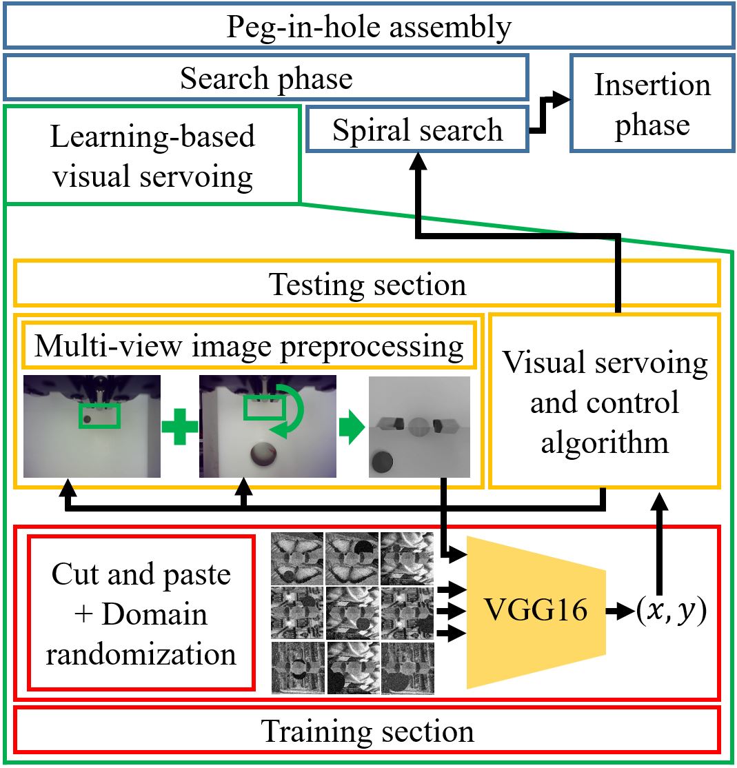
This leads us to study how to quickly assemble pegs into uncertain holes on surfaces with different colors and textures. We develop a peg-in-hole assembly system that uses learning-based visual servoing to quickly move the peg closer to the hole, uses spiral search to precisely align the peg and the hole, and uses impedance control to fully insert the peg into the hole. Fig.1 shows the outline of the developed peg-in-hole program. The search phase comprises the learning-based servoing and spiral search. The insertion phase comprises the impedance control.

Specifically, our main contribution is the learning-based visual servoing. We use synthesized data to train a deep neural network to predict the position of a hole, and use iterative visual servoing to iteratively moves a peg towards the hole.

Various experiments and analysis using both simulation and real-world experiments are performed to (1) analyze the performance of the learning-based visual servoing against uncertain holes on surfaces with different colors and textures, and (2) compare the efficiency of executions under different initial hole positions. The results show that the proposed method is robust to various surface backgrounds and can generally speed up the entire peg-in-hole process.

II Related Work

This paper focuses on the problem of peg-in-hole assembly using deep learning. Thus, this section reviews the related work in peg-in-hole assembly and the applications of deep learning in industrial robots.

II-A Peg-in-hole assembly

Peg-in-hole assembly refers to the task of inserting a peg to a hole. The task generally has two phases – the search phase and the insertion phase. The insertion phase refers to the phase when the peg is being inserted, and it has been studied extensively. The search phase is the stage of finding a hole when position uncertainty exceeds the clearance of a hole. It is less studied.

II-A1 Insertion phase

One of the earliest studies about the insertion phase is Shirai and Inoue[1], where they used visual feedback to perform insertion. About a decade later, researchers shifted from the use of visual feedback to the use of compliance to accommodate the motion of the end-effector during insertion[2][3][4][5]. In the 1990s, the quasi-static contact analysis was used to guide the insertion[6][7][8]. The state-of-the-art method for insertion is impedance control[9][10]. It is widely used in many practical systems.

II-A2 Search phase

The search phase is before the insertion and is used to align the peg and the hole. Below, related work about the search phase, sometimes followed by insertion, is reviewed. The studies can generally be categorized by the types of sensors used: vision sensors, force sensors, or both.

The first category uses vision sensors. Yoshimi and Allen[11] dealt with visual uncertainty for peg-in-hole by attaching a camera to the end-effector and rotating the camera around the last axis of the robot. Morel et al.[12] employed 2D visual servoing (search phase) followed by force control (insertion phase) to successfully performed peg-in-hole assembly with large initial offsets. Huang et al.[13] used high-speed cameras to align a peg to a hole. More recently, the visual coaxial system was used to perform precise alignment in peg-in-hole assembly[14][15].

The second category uses force-torque sensors. Newman et al.[16] proposed the use of force/torque maps to guide the robot to the hole. Sharma et al.[17] generalized the work of Newman et al.[16] to tilted pegs. Chhatpar and Branicky[18] explored various blind search methods such as tilting and covering the search space using paths like spiral path (a.k.a. spiral search). Spiral search and its variants were also discussed in [19][20]. The problem of spiral search is that it is time consuming, given that the robot just blindly searches for the hole. Tilting, often considered as a method intuitive to human, was also explored in several studies[20][21][22][23]. The limitation of tilting is that it assumes that the initial offset is small.

More recently, studies such as [24] used a combination of visual sensors and force-torque sensors to track the uncertainties of object poses and sped up the search process. This paper similarly employs both visual sensors and a force-torque sensor. Specifically, we explore the use of a combination of visual servoing using two in-hand RGB cameras, followed by the spiral search using force sensors, to perform a peg-in-hole assembly.

II-B Deep learning in industrial robotics

Deep learning has in the recent years gained prominence in robotics. Some studies used real-world data to train deep neural networks. For example, Pinto and Gupta[25] collected 700 robot hours of data and used them to train a robot to grasp objects. Levine et al.[26] similarly made robots perform bin-picking randomly for days, before finally using the data obtained to train a deep network for bin-picking. Inoue et al.[27] proposed deep reinforcement networks for precise assembly tasks. Lee et al.[28] trained multimodal representations of contact-rich tasks and trained a robot to perform peg-in-hole. Thomas et al.[29] used CAD data to help improve the performance of end-to-end learning for robotic assembly. Yang et al.[30] and Ochi et al.[31] took data by performing teleoperations and used them to make the robot learn specific motions. De Magistris et al.[32] took labeled force-torque sensor data to train a robot to perform multi-shape insertion. Although the aforementioned studies showed the possibilities of using real-world data, developing such systems are difficult. Collecting and labeling the real-world data is time-consuming and labor intensive.

For this reason, robotic searchers began to study training deep neural networks using synthesized data. Dwibedi et al.[33] cut and pasted pictures of objects on random backgrounds to train deep neural networks for object recognition. Mahler et al.[34] used synthetic data of depth images to train robots for bin-picking. Unfortunately, the use of synthetic data is limited due to reality gap[35].

To overcome the reality gap, one method is transfer learning [36]. Domain adaptation is an example of transfer learning, where synthetic data and real-world data are both used[37][38] [39][40]. Domain randomization highly promotes the use of synthesized data[41][42]. It suggests that synthetic data with randomization can be helpful to allow transfer without the need for real-world data. Using domain randomization in data synthesis were widely studied[43][44][45][46].

The learning-based visual servoing of this work is based on domain randomization. It is used to synthesize the training data for a deep neural network. It is also used to synthesize various testing data sets to analyze the performance of the neural network.

III Methods

This section gives a general explanation of the proposed peg-in-hole assembly method, with a special focus on the learning-based visual servoing, and the synthetic data generation.

III-A Overview of the proposed peg-in-Hole assembly

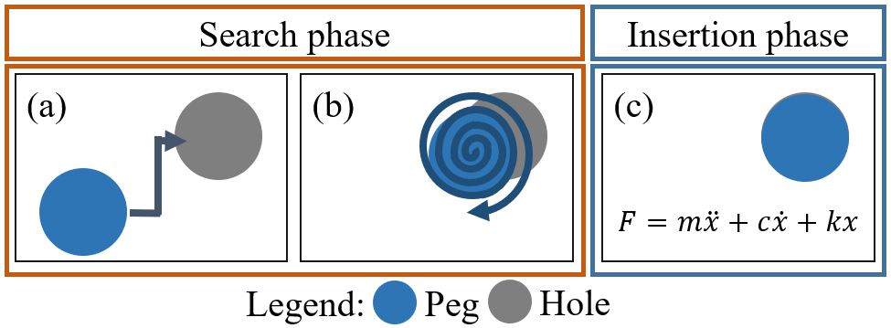
The work flow of the proposed method is shown in Fig.2. It includes a search phase (Fig.2(a, b)) and an insertion phase (Fig.2(c)). The search phase has two steps: Learning-based visual servoing (Fig.2(a)) and spiral search (Fig.2(b)). The learning-based visual servoing quickly moves a peg closer to the hole, while the spiral search can precisely align the peg and the hole.

Figure 2: The proposed peg-in-hole assembly includes two phases: A search phase and an insertion phase. The search phase has two steps: (a) Learning-based visual servoing and (b) Spiral search. They move and align the peg to the hole. The insertion phase uses (c) impedance control to insert the peg into the hole.

Figure 3: Definition of the coordinate systems $\Sigma_{eef}$, $\Sigma_{img}$, and $\Sigma_{spiral}$. (The definition is for the image captured by Camera 1. For the other camera discussed later, the coordinate system reverses.)

The details of the learning-based visual servoing will be discussed in Section III-B. It is the main contribution of the work.

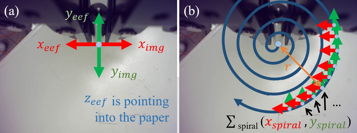
The spiral search is conducted along the $xy$-plane of the end-effector coordinate system $\Sigma_{eef}(x_{eef},y_{eef})$, shown in Fig.3. The reference coordinate system for spiral search $\Sigma_{spiral}(x_{spiral},y_{spiral})$ is of the same orientation as $\Sigma_{eef}$ with the origin $r$ away from the initial peg position. The path for spiral search is given in Eqn.(1).

$$x_{spiral}=r\cos{\theta},y_{spiral}=r\sin{\theta}$$ (1)

where $\theta$ and $r$ start from 0. $\theta$ increases by $\delta\theta$ every timestep, while $r$ increases for $\delta$$r$ for every 1 full rotation. The robot will move following the discrete spiral path described above, and continue until the force at the -$z$ direction of $\Sigma_{eef}$ is less than $F_{max}$ or $r$ reaches a predefined threshold.

The assembly switches to the insertion phase when the condition for the -$z$ direction force is fulfilled. Impedance control is used to perform insertion in the insertion phase.

III-B Learning-based visual servoing

The learning-based visual servoing uses (1) a deep neural network and multi-view images to predict the position of the hole and (2) continuous visual servoing to move the peg towards the hole.

III-B1 Predicting the position of the hole

We train a neural network that can map an image $I$ to an output of ($x$,$y$), where ($x$,$y$) indicates the distance between the center of the peg and the hole as seen in the image in pixels on coordinate system $\Sigma_{img}$ shown in Fig.3.

Figure 4: VGG-16 network architecture [47] used in the proposed method.

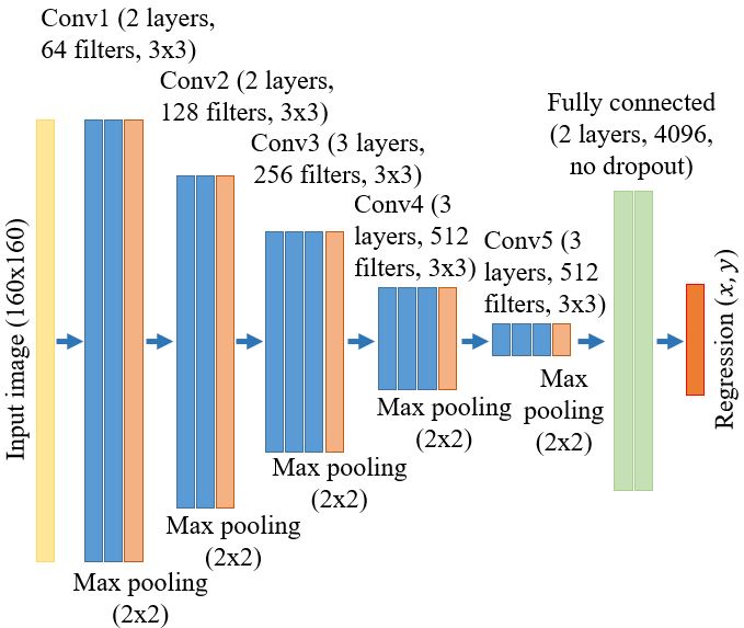
VGG-16 network is used following the suggestion of [42]. The VGG-16 network is adjusted for regression instead of classification. The input of the network is adjusted to a grayscale image of size 160$\times$160. The output is a predicted hole position ($x$,$y$). Fig.4 shows the diagram of the VGG-16 network. Following [42], the dropout components of the network are removed to avoid local minima. The network is trained using Adam, with settings following [48]. Mean squared error (MSE) is selected as the loss function.

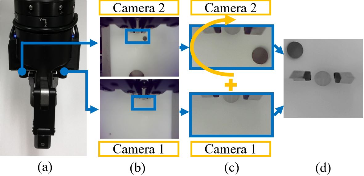
The input image is a concatenation of two images from two in-hand cameras installed on two sides of a robot hand. Fig.5 shows the concatenation. To define the size of the cropped image, a bounding box of size 160$\times$80 around the center of the peg is predefined, such that the concatenated image reaches 160$\times$160.

Figure 5: Concatenating two multi-view images into the input image to the VGG-16 network. (a) Configurations of the two in-hand cameras. (b) An area around the center of the peg of each image is cropped. (c-d) Concatenate the cropped area into a 160$\times$160 image.

III-B2 Iterative visual servoing

While the network outputs ($x$,$y$) in pixels, the image is not exactly a 2D image parallel to the surface of where the hole is. Thus, instead of directly moving the peg to the predicted position, we use the $\operatorname{sgn}$ function to classify the outputted values into 4 quadrants, as shown in Fig.6, and iteratively moves the peg towards the quadrants.

Figure 6: Definition of the quadrants. Top images show how the gripper and the hole are relatively positioned from a front view. The bottom images are the concatenated image from the two cameras. (a) Quadrant ”Topleft”. (b) Quadrant ”Bottomleft”. (c) Quadrant ”Bottomright”. (d) Quadrant ”Topright”.

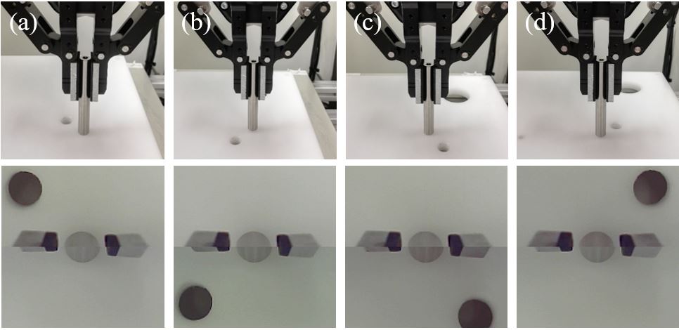
Consider the coordinate system $\Sigma_{h}$ which shares the same orientation as $\Sigma_{eef}$ and has an origin at the center of the hole. Assuming at discrete timestep $t$, where $t$ is a non-negative integer that starts from 0, the peg is located at ($x_{h}[t]$,$y_{h}[t]$) and the values outputted by the trained network is ($x[t]$,$y[t]$). We can move the peg closer with only the quadrant information using Eqn.(2).

$$\begin{bmatrix}x_{h}[t+1]\\ y_{h}[t+1]\end{bmatrix}=\begin{bmatrix}x_{h}[t]\\ y_{h}[t]\end{bmatrix}-\lambda[t]\begin{bmatrix}-\operatorname{sgn}(x[t])\\ -\operatorname{sgn}(y[t])\end{bmatrix}$$ (2)

where $\lambda$ (unit=$mm$/px) is a time dependent coefficient with decreasing values and converges to 0 along with time. $\lambda$ is defined as:

$$\lambda[t]=\frac{A(n-t)}{n}$$ (3)

where $A$ is the maximum allowable relative moving distance. $\lambda[t]$ converges to 0 at time $n$. By repeating this for $n_{run}$ times, where $n_{run}<n$, the peg will get closer to the center of the hole as long as the quadrant the hole is at relative to the peg can be correctly predicted by the deep neural network. The method is robust to the prediction errors of the deep neural network since it is not directly using the predicted numbers.

III-C Synthetic Data Generation Method

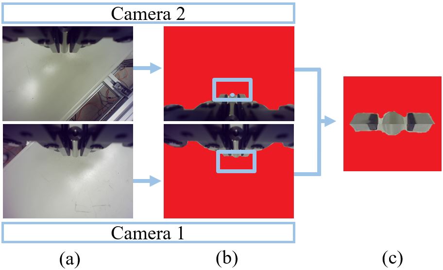
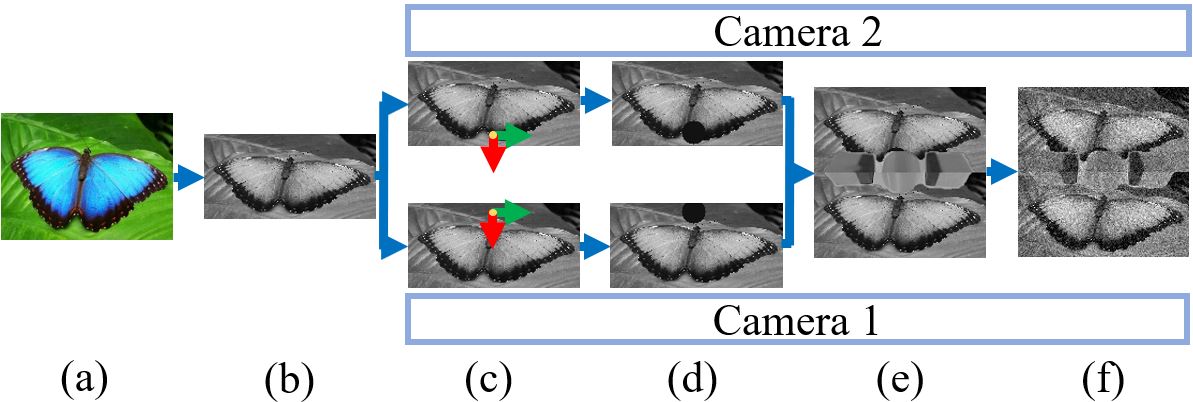
Synthetic data generation is used to get a large amount of training. The basic idea is to change the background of the cameras with various images. First, we get a gripper template mask following Fig.7. The purpose of having a gripper template mask is to simulate the view of the gripper in the cameras. Then, the gripper template mask is attached to some random images with a circle (the hole) to make a synthesized assembly data. Fig.8 shows attaching process. There are four kinds of randomization in the attaching. (1) The background of the image is randomized. (2) The size of the circle (the hole) is randomized. (3) The darkness of the circle (the hole) is randomized. (4) Gaussian noises are added to randomize the gripper template mask. By using random background images captured from the Internet and likening the hole to a dark-colored circle, a large number of synthetic images with known labels ($x$,$y$) can be quickly synthesized.

Figure 7: Obtaining the gripper template mask for generating synthetic data. (a) The images from the in-hand cameras. (b) Rotate the image from camera 2, mark the gripper mask, locate the center of the peg, and define the bounding box on each image. (c) Crop the image according to the bounding box and concatenate.

Figure 8: Attaching the gripper template mask to some random images with a circle (the hole) to make a synthesized assembly data. The hole is added to the background image in (d). The gripper template mask is added in (e). Gaussian noises are added in (f).

IV Experiments

The experiments section is divided into two parts. In the first part, we compare and analyze the performance of the neural network under different training data. In the second part, we analyze the real-world visual servoing and insertions using the best performing network.

IV-A Performance of the neural network

The specification of the computer used for the neural network is Intel(R) Core(TM) I5-6500 @3.20 GHz, 16GB RAM, with an Nvidia Geforce GTX 1080 card.

IV-A1 Training data

The synthetic training data was generated using the method described in Section III-C. Six categories of random images were prepared, as shown in Fig.9. 776 positions (194 positions per quadrant) are evenly sampled in each image to define the position of a hole. These positions have a maximum of 4 $cm$ uncertainty (the range is [-66 px, 66 px]). The darkness of a hole was randomized in range [10, 70] (0 is fully black, 255 is fully white). The diameter of a hole (in pixels) was randomized in range [10 px , 35 px] (around [3 $cm$, 1 $cm$]). In total, we generated 69,840 synthetic images using each category of random images. It took an average time of 22 minutes without using the Graphics Processing Unit (GPU).

Figure 9: Six categories of randomly collected images are used for synthesizing the training data. Images of category ”Plain” is generated manually. The rest are downloaded from the Internet using category names as the search keywords.

The details of the synthesis are as follows. Using the six categories of images, we synthesized 9 sets of training data. They are “Plain”, “Image”, “Textures+Scenery(18)”, “Textures+Scenery(30)”, “Textures+Scenery(45)”, “Textures+Scenery(90)”, “Textures(45)”, “Metallic(45)”, “Scenery(45)”. For the “Plain” training set, the background images were randomly selected from the “Plain” category, resulting into 69,840 synthetic images with background color ranges [0,255]. For the “Image” training set, the background images were randomly selected from the “Image” category where 776 random images searched using the keyword “Image” were downloaded. For the “Textures(45)”, “Scenery(45)”, and “Metallic(45)” training set, 45 images randomly selected from their corresponding categories. For the “Textures+Scenery(45)” training set, 22 images from the “Textures” category and 23 images from the “Scenery” category were randomly selected and combined. The “Textures+Scenery(18)”, “Textures+Scenery(30)”, and “Textures+Scenery(90)” training data sets were prepared similarly to ”Textures+Scenery(45)”, except that different number of images (9-9, 15-15, and 45-45 respectively) were selected from the corresponding categories. Images from the “Food” category were not used in the training data. They were prepared for testing.

IV-A2 Testing data

Generation of testing data was done similarly, except with 584 random positions instead of 776. In total, 6 sets of testing data were prepared. They are “Plain”, “Light plain”, “Textures”, “Metallic”, “Scenery”, and “Food”. The background images of these testing data set were randomly selected from their corresponding categories. Especially, for the ”Light plain” testing set, 35 different colors of range [125,255] were selected instead of [0,255], making it different from the “Plain” testing set.

IV-A3 Training

Several different VGG-16 networks were trained and compared using the various training data sets. The names of the networks are the same as the training data sets to clearly show the correspondence. The parameter settings of the VGG-16 neural network was shown in Fig.4. The initial weights were random. The learning rate was set to 1e-5. The training data set used for each network was divided by a ratio of 8:2 for training and validation. The epoch was set to 40. Convergence was faster for less random images (“Plain”, “Textures”, “Metallic surface”). The loss at the end of epoch 40 for these less varied image categories was also smaller, albeit overfitting existed in all trained networks, similar to [42]. Each training time was on average 11 hours.

IV-A4 Results

Table I shows the results of the trained networks and their performance on the 6 sets of testing data.

TABLE I: Performance of the VGG-16 networks

Training data set	Testing data set	$MSE_{all}$	$MSE_{no_{o}utlier}$	$R_{outlier}$	$R_{quadrant}$
Plain	Plain	95.0	5.0	0.054	0.951
Plain	Light plain	0.4	0.4	0.000	0.999
Plain	Textures	620.1	17.2	0.368	0.721
Plain	Metallic	609.0	29.2	0.383	0.715
Plain	Scenery	1396.9	72.3	0.791	0.405
Plain	Food	1133.5	77.5	0.744	0.479
Image	Plain	396.3	12.3	0.216	0.819
Image	Light plain	4.2	3.8	0.001	0.992
Image	Textures	185.9	13.0	0.114	0.911
Image	Metallic	134.4	11.7	0.072	0.935
Image	Scenery	119.1	13.6	0.070	0.940
Image	Food	101.0	13.2	0.065	0.934
Textures+Scenery(18)	Plain	511.9	13.6	0.282	0.755
Textures+Scenery(18)	Light plain	2.3	2.0	0.0004	0.995
Textures+Scenery(18)	Textures	352.9	15.9	0.199	0.829
Textures+Scenery(18)	Metallic	329.6	16.2	0.158	0.854
Textures+Scenery(18)	Scenery	288.5	19.8	0.158	0.862
Textures+Scenery(18)	Food	322.9	25.9	0.221	0.824
Textures+Scenery(30)	Plain	414.0	9.7	0.244	0.791
Textures+Scenery(30)	Light plain	0.99	0.99	0.000	0.998
Textures+Scenery(30)	Textures	241.1	10.2	0.140	0.884
Textures+Scenery(30)	Metallic	225.3	11.0	0.112	0.903
Textures+Scenery(30)	Scenery	196.4	13.1	0.107	0.909
Textures+Scenery(30)	Food	298.2	17.5	0.191	0.845
Textures+Scenery(45)	Plain	399.2	13.4	0.259	0.804
Textures+Scenery(45)	Light plain	2.9	2.3	0.001	0.994
Textures+Scenery(45)	Textures	378.9	14.4	0.210	0.826
Textures+Scenery(45)	Metallic	359.8	14.5	0.173	0.855
Textures+Scenery(45)	Scenery	332.1	18.9	0.176	0.849
Textures+Scenery(45)	Food	511.0	23.0	0.285	0.772
Textures+Scenery(90)	Plain	447.2	12.1	0.280	0.780
Textures+Scenery(90)	Light plain	9.3	3.9	0.006	0.984
Textures+Scenery(90)	Textures	389.2	13.1	0.213	0.835
Textures+Scenery(90)	Metallic	341.0	13.8	0.166	0.863
Textures+Scenery(90)	Scenery	345.6	16.7	0.185	0.857
Textures+Scenery(90)	Food	380.2	17.6	0.210	0.828
Textures(45)	Plain	383.4	11.0	0.234	0.807
Textures(45)	Light plain	1.9	1.9	0.000	0.992
Textures(45)	Textures	315.7	12.3	0.167	0.860
Textures(45)	Metallic	310.1	14.2	0.151	0.863
Textures(45)	Scenery	369.0	18.6	0.185	0.837
Textures(45)	Food	457.3	26.9	0.287	0.781
Metallic(45)	Plain	495.8	12.5	0.299	0.766
Metallic(45)	Light plain	7.4	3.2	0.006	0.991
Metallic(45)	Textures	409.5	12.8	0.241	0.814
Metallic(45)	Metallic	350.9	15.0	0.192	0.858
Metallic(45)	Scenery	450.7	19.0	0.244	0.808
Metallic(45)	Food	514.0	22.0	0.282	0.775
Scenery(45)	Plain	500.0	14.4	0.282	0.769
Scenery(45)	Light plain	11.7	4.6	0.007	0.992
Scenery(45)	Textures	318.7	15.3	0.203	0.862
Scenery(45)	Metallic	310.4	16.0	0.174	0.877
Scenery(45)	Scenery	285.2	18.9	0.172	0.890
Scenery(45)	Food	395.4	21.0	0.236	0.836

• $MSE_{all}$: Mean squared error on all images of the testing dataset; $MSE_{no_{o}utlier}$: Mean squared error of images of the testing dataset, excluding the outliers; $R_{outlier}$: Ratio of image classified as outliers (images with a mean squared error of more than 200); $R_{quadrant}$: Ratio of images correctly classified into its corresponding quadrants.

The results show that the ${MSE}_{all}$ on most testing data sets are quite large. The reason is because of the existence of outliers (the images which predicted outputs are completely off from the true outputs). Without counting the outliers, the MSE ($MSE_{no\_outlier}$) drops significantly. Thus, to minimize the effect of the outliers, the quadrants and iterative visual servoing method explained in section III-B was adopted.

Fig.10 shows how the use of images instead of plain backgrounds improves the network’s robustness. There is an increase in average performance ($R_{quadrant}$ of Table I) on all testing data sets. The network trained with the “Plain” data set performs better on the “Plain” testing data set due to overfitting, especially in cases where backgrounds have similar darkness to the hole.

Figure 10: Performance of the networks trained with the “Plain” and “Image” data set. The vertical axis is the $R_{quadrant}$ of Table I in %.

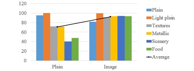
Fig.11 shows the $R_{quadrant}$ of the “Metallic(45)”, “Textures+Scenery(45)”, “Textures(45)”, and “Scenery(45)” training sets. The comparison indicates that: (1) With exception on the “Light plain”, the networks trained with a certain data set generally perform better on similar test sets. (2) Networks trained on certain data sets cannot perform as well on a background with high randomness like the “Food” test set. Thus, training with images of a certain data set can improve the network’s performance on similar test sets. On the other hand, for categories with less variety like “Metallic” or “Textures” (less than “Food”), improvements on the network performance can be obtained by training on data of higher variety, like “Scenery”. This is from the observation that the network trained with “Scenery” performs similarly to the one trained with “Textures” on the “Textures” test set, and performs better compared to the networks trained with “Metallic” on the “Metallic” test set.

Figure 11: Performance the networks trained with “Metallic(45)”, “Textures+Scenery(45)”, “Textures(45)”, and “Scenery(45)” training sets. The vertical axis is the $R_{quadrant}$ of Table I in %.

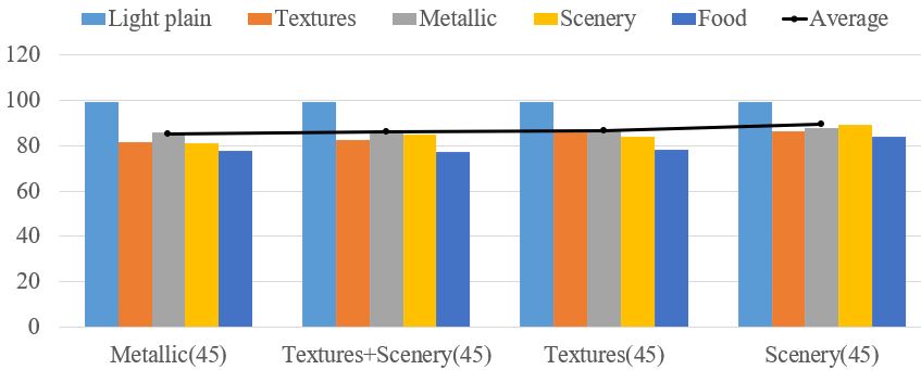
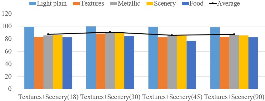
Fig.12 compares the performance of networks trained data sets synthesized with different numbers of similar background images. The results imply that the number is not the only crucial parameter. Other forms of randomization including hole sizes and hole darkness also play important roles in the synthesis of the training data.

Figure 12: Performance of the networks trained with “Textures+Scenery” data sets synthesized with different numbers of similar background image. The vertical axis is the $R_{quadrant}$ of Table I in %.

IV-B Real-world Experiments

We performed real-world experiments using the networks trained with the “Image” data set and the “Plain” data set, for they have the best and worst performance. Four different surfaces, as is shown in Fig.13, were used in the experiments. A success execution is judged to be when the peg is inserted within 90 sec.

Figure 13: The four surfaces used in real-world experiments. (a) White. (b) Brown. (c) Pink. (d) Sky.

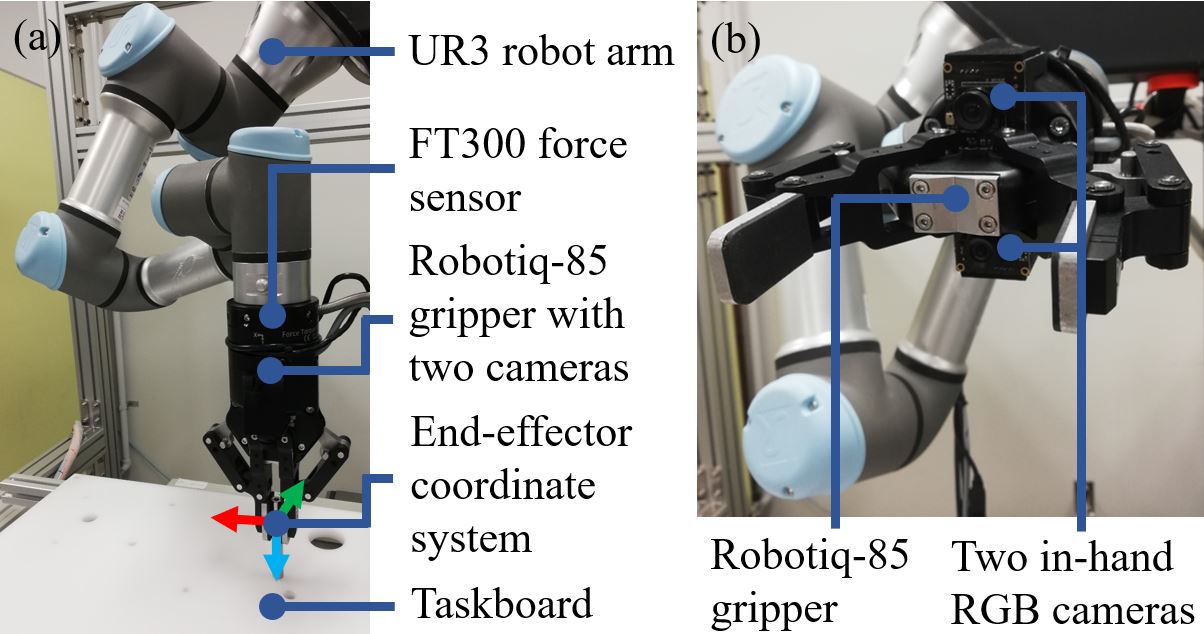
The robot we used to do real-world experiments is a UR3 robot with a FT300 force sensor and a Roboti-85 gripper. Two in-hand cameras were used to collect multi-view images. Fig.14 shows the experimental setup. The robot was made to insert a 75$\times$10 $mm$ peg into a hole. The taskboard in the left of Fig.14 is the base with the hole to be inserted. The lenience of the hole for the experiment is 0.4$mm$. The specification of the computer used was the same as the one used to train the deep neural network.

Figure 14: The experimental setup. (a) The overall view on the experimental setup. (b) A close-up view of the Robotiq-85 gripper with the two in-hand RGB cameras.

The parameters for the spiral search were $r_{init}$=0.3$mm$, $r_{max}$=7.0$mm$, $\delta\theta$=12.5^∘, $\delta$$r$=0.3$mm$, and $F_{max}$=20$N$. The parameters for the iterative visual servoing were $A$=10$mm$, $n$=10, $n_{run}$=5. The parameters of the impedance control were $c$ = [50,50,50,1,1,1] for the damper and $k$ = [100,100,100,100,100,100] for the spring.

Table II shows the success rates of the real-world experiments. Ten times of trial are performed for each training set and testing surface combination. The network trained with the “Image” data set can successfully ignore the variations of the “White”, “Brown”, and “Pink” surfaces and correctly predict the correct quadrants. Fig.15(a) shows an example of the success sequence on the “Pink” surface. The network trained with “Plain” can also correctly predict the quadrant and successfully performs insertion on the “White” and “Brown” surfaces. Although a few overshoots were spotted, the quadrant-based visual servoing compensated them after several iterations. An example is shown in Fig.15(b).

TABLE II: Performance of the real-world experiments

Network name	$R_{white}$	$R_{brown}$	$R_{pink}$	$R_{sky}$
Image	10/10 ($\oplus$)	10/10 ($\oplus$)	10/10 ($\oplus$)	3/10 ($\bigtriangleup$)
Plain	10/10 ($\ominus$)	10/10 ($\ominus$)	4/10 ($\bigtriangleup$)	0/10 ($\times$)

• $R_{white}$: Ratio of successful insertions on the “White” surface; $R_{brown}$: Ratio of successful insertions on the “Brown” surface; $R_{pink}$: Ratio of successful insertions on the “Pink” surface; $R_{sky}$: Ratio of successful insertions on the “Sky” surface; $\oplus$: The deep network gives output of the correct quadrant; $\ominus$: The deep network successfully predicts the correct quadrant; $\bigtriangleup$: The deep network sometimes successfully predicts the correct quadrant; $\times$: The deep network rarely successfully predicts the correct quadrant.

TABLE III: Time cost under different initial position errors

$D_{euclidean}$	$t_{with-visual}$	$t_{without-visual}$
23.8	30.4	$>$90.0
15.0	33.4	$>$90.0
12.0	41.3	$>$90.0
11.7	47.2	$>$90.0
10.0	70.1	$>$90.0
12.5	39.0	$>$90.0
11.0	63.4	$>$90.0
14.1	22.8	$>$90.0
4.0	56.1	25.5
13.6	43.4	$>$90.0

• $D_{h,euclidean}$: Initial distance from the center of the peg o the center of the hole in $mm$; $t_{with-visual}$: Time taken from the start of the search phase until the end of the insertion using the proposed method in sec. (network trained using “Image”); $t_{with-visual}$: Time taken from the start of the search phase until the end of insertion with a simple spiral search in sec.

Figure 15: Some snapshots of the real-world executions from the results shown in Table II. (a) A successful execution using the network trained with “Image” and tested on the “Pink” surface ($\oplus$ category). (b) A successful execution (with overshoots) using the network trained with “Plain” and tested on the “White” surface ($\ominus$ category). (c) A failure case using the network trained with “Image” and tested on the “Sky” surface ($\bigtriangleup$ category). (d) A failure case using the network trained with “Plain” and tested on the “Sky” surface ($\times$ category).

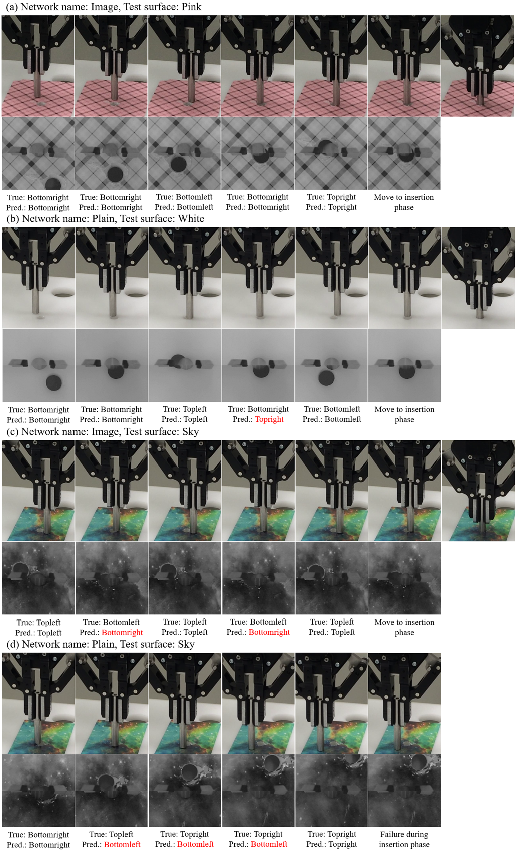
The failure appears with the “Sky” surface for both networks and the “Pink” surface for the network trained with the “Plain” data set. For the network trained with the “Image” data set and examined using the “Sky” surface and the network trained with the “Plain” data set and examined using the “Pink” surface, errors sometimes occur, resulting into 3/10 and 4/10 success rates in Table II respectively. Fig.15(c) shows an example of the failure sequence. For the network trained with the “Plain” data set and examined using the “Sky” surface, the success rate is 0/10. Fig.15(d) is an example of the failure.

Table III compares the time cost of 10 executions on the “White” surface with and without the learning-based visual servoing. The initial positions errors were randomly set (as is shown in the first column of Table III). When the initial position error is large, the robot system could finish an insertion in less than 70 sec. with the learning-based visual servoing. In contrast, the execution costs larger than 90 sec. or fails. An exception is $D_{euclidean}$=4.0$mm$. In this case, the initial position error is small. A simple spiral search could quickly find the hole. The result demonstrates that the proposed method improves search efficiency when the position of the hole has large uncertainty.

V Conclusions

In conclusion, we developed a learning-based visual servoing method to quickly insert pegs into uncertain holes. The method used a deep neural network trained on synthetic data to predict the quadrant of a hole, and used iterative visual servoing to move the peg towards the hole step by step. The synthetic data was generated by cutting and pasting gripper template masks on random images, which allowed extremely fast synthetic data generation. Performance of different training data sets was compared. Training with images from categories of higher variety can lead to better performance, even for testing with images from categories of less variety. Real-world experiments showed that the proposed method is robust to various surface backgrounds. The system is generally faster compared to a peg-in-hole assembly using only a spiral search, unless the initial error is very small.

References

- [1] Y. Shirai and H. Inoue, “Guiding a robot by visual feedback in assembling tasks.” Pattern Recognition, vol. 5, no. 2, pp. 99–106, 1973.
- [2] D. E. Whitney, “Quasi-static assembly of compliantly supported rigid parts,” J. Dyn. Sys., Meas., Control., vol. 104, no. 1, pp. 65–77, 1982.
- [3] M. T. Mason, “Compliance and force control for computer controlled manipulators,” IEEE Trans. Syst., Man, Cybern., vol. 11, no. 6, pp. 418–432, 1981.
- [4] L. Balletti et al., “Towards variable impedance assembly: the vsa peg-in-hole,” in ICHR, 2012, pp. 402–408.
- [5] X. Zhang, Y. Zheng, J. Ota, and Y. Huang, “Peg-in-hole assembly based on two-phase scheme and f/t sensor for dual-arm robot,” Sensors, vol. 17, no. 9, p. 2004, 2017.
- [6] P. Nguyen and F. Naghdy, “Fuzzy control of automatic peg-in-hole insertion,” in ANZIIS, 1995, pp. 134–139.
- [7] I.-W. Kim et al., “Active peg-in-hole of chamferless parts using force/moment sensor,” in IROS, vol. 2, 1999, pp. 948–953.
- [8] J. Su et al., “Sensor-less insertion strategy for an eccentric peg in a hole of the crankshaft and bearing assembly,” Assembly Automation, vol. 32, no. 1, pp. 86–99, 2012.
- [9] J. F. Broenink and M. L. Tiernego, “Peg-in-hole assembly using impedance control with a 6 dof robot,” in European Simulation Symposium, 1996, pp. 504–508.
- [10] H.-C. Cho et al., “A strategy for connector assembly using impedance control for industrial robots,” in ICCAS, 2012, pp. 1433–1435.
- [11] B. H. Yoshimi and P. K. Allen, “Active, uncalibrated visual servoing,” in ICRA, 1994, pp. 156–161.
- [12] G. Morel et al., “Impedance based combination of visual and force control,” in ICRA, vol. 2, 1998, pp. 1743–1748.
- [13] S. Huang et al., “Fast peg-and-hole alignment using visual compliance,” in IROS, 2013, pp. 286–292.
- [14] P. Nagarajan et al., “Vision based pose estimation of multiple peg-in-hole for robotic assembly,” in ICVGIP, 2016, pp. 50–62.
- [15] Z. Yang et al., “A coaxial vision assembly algorithm for un-centripetal holes on large-scale stereo workpiece using multiple-dof robot,” in IST, 2018, pp. 1–6.
- [16] W. S. Newman et al., “Interpretation of force and moment signals for compliant peg-in-hole assembly,” in ICRA, 2001, pp. 571–576.
- [17] K. Sharma et al., “Intelligent and environment-independent peg-in-hole search strategies,” in CARE, 2013, pp. 1–6.
- [18] S. R. Chhatpar and M. S. Branicky, “Search strategies for peg-in-hole assemblies with position uncertainty,” in IROS, vol. 3, 2001, pp. 1465–1470.
- [19] I. F. Jasim et al., “Position identification in force-guided robotic peg-in-hole assembly tasks,” Procedia Cirp, vol. 23, pp. 217–222, 2014.
- [20] J. A. Marvel et al., “Multi-robot assembly strategies and metrics,” ACM Computing Surveys, vol. 51, no. 1, p. 14, 2018.
- [21] H. Park et al., “Intuitive peg-in-hole assembly strategy with a compliant manipulator,” in ISR, 2013, pp. 1–5.
- [22] I. F. Jasim and P. W. Plapper, “Contact-state monitoring of force-guided robotic assembly tasks using expectation maximization-based gaussian mixtures models,” Int J Adv Manuf Tech, vol. 73, no. 5-8, pp. 623–633, 2014.
- [23] M. W. Abdullah et al., “An approach for peg-in-hole assembling using intuitive search algorithm based on human behavior and carried by sensors guided industrial robot,” IFAC-PapersOnLine, vol. 48, no. 3, pp. 1476–1481, 2015.
- [24] H. Nguyen and Q.-C. Pham, “A probabilistic framework for tracking uncertainties in robotic manipulation,” arXiv preprint arXiv:1901.00969, 2019.
- [25] L. Pinto and A. Gupta, “Supersizing self-supervision: Learning to grasp from 50k tries and 700 robot hours,” in ICRA, 2016, pp. 3406–3413.
- [26] S. Levine et al., “Learning hand-eye coordination for robotic grasping with deep learning and large-scale data collection,” IJRR, vol. 37, no. 4-5, pp. 421–436, 2018.
- [27] T. Inoue et al., “Deep reinforcement learning for high precision assembly tasks,” in IROS, 2017, pp. 819–825.
- [28] M. A. Lee et al., “Making sense of vision and touch: Self-supervised learning of multimodal representations for contact-rich tasks,” arXiv preprint arXiv:1810.10191, 2018.
- [29] G. Thomas et al., “Learning robotic assembly from cad,” arXiv preprint arXiv:1803.07635, 2018.
- [30] P.-C. Yang et al., “Repeatable folding task by humanoid robot worker using deep learning,” IEEE Robot. Autom. Lett., vol. 2, no. 2, pp. 397–403, 2017.
- [31] H. Ochi et al., “Deep learning scooping motion using bilateral teleoperations,” in ICARM, 2018, pp. 118–123.
- [32] G. De Magistris et al., “Experimental force-torque dataset for robot learning of multi-shape insertion,” arXiv preprint arXiv:1807.06749, 2018.
- [33] D. Dwibedi et al., “Cut, paste and learn: Surprisingly easy synthesis for instance detection,” in ICCV, 2017.
- [34] J. Mahler et al., “Dex-net 3.0: Computing robust robot vacuum suction grasp targets in point clouds using a new analytic model and deep learning,” arXiv preprint arXiv:1709.06670, 2017.
- [35] N. Jakobi et al., “Noise and the reality gap: The use of simulation in evolutionary robotics,” in ECAL, 1995, pp. 704–720.
- [36] S. J. Pan, Q. Yang et al., “A survey on transfer learning,” IEEE Trans. Knowl. Data Eng., vol. 22, no. 10, pp. 1345–1359, 2010.
- [37] G. Csurka, “Domain adaptation for visual applications: A comprehensive survey,” arXiv preprint arXiv:1702.05374, 2017.
- [38] F. Zhang et al., “Adversarial discriminative sim-to-real transfer of visuo-motor policies,” arXiv preprint arXiv:1709.05746, 2017.
- [39] K. Bousmalis et al., “Using simulation and domain adaptation to improve efficiency of deep robotic grasping,” in ICRA, 2018, pp. 4243–4250.
- [40] K. Fang et al., “Multi-task domain adaptation for deep learning of instance grasping from simulation,” in ICR, 2018, pp. 3516–3523.
- [41] F. Sadeghi and S. Levine, “Cad2rl: Real single-image flight without a single real image,” arXiv preprint arXiv:1611.04201, 2016.
- [42] J. Tobin et al., “Domain randomization for transferring deep neural networks from simulation to the real world,” in IROS, 2017, pp. 23–30.
- [43] J. Tremblay et al., “Training deep networks with synthetic data: Bridging the reality gap by domain randomization,” arXiv preprint arXiv:1804.06516, 2018.
- [44] M. Andrychowicz et al., “Learning dexterous in-hand manipulation,” arXiv preprint arXiv:1808.00177, 2018.
- [45] A. Prakash et al., “Structured domain randomization: Bridging the reality gap by context-aware synthetic data,” arXiv preprint arXiv:1810.10093, 2018.
- [46] M. Sundermeyer and Others, “Implicit 3d orientation learning for 6d object detection from rgb images,” in ECCV. Springer, 2018, pp. 712–729.
- [47] K. Simonyan and A. Zisserman, “Very deep convolutional networks for large-scale image recognition,” arXiv preprint arXiv:1409.1556, 2014.
- [48] D. P. Kingma and J. Ba, “Adam: A method for stochastic optimization,” arXiv preprint arXiv:1412.6980, 2014.