Science with the TianQin observatory: Preliminary results on testing the no-hair theorem with ringdown signals
Abstract
We study the capability of the space-based gravitational wave observatory TianQin to test the no-hair theorem of General Relativity, using the ringdown signal from the coalescence of massive black hole binaries. We parameterize the ringdown signal by the four strongest quasinormal modes and estimate the signal to noise ratio for various source parameters. We consider constraints both from single detections and from all the events combined throughout the lifetime of the observatory, for different astrophysical models. We find that at the end of the mission, TianQin will have constrained deviations of the frequency and decay time of the dominant 22 mode from the general relativistic predictions to within 0.2 % and 1.5 % respectively, the frequencies of the subleading modes can be also constrained within 0.3%. We also find that TianQin and LISA are highly complementary, by virtue of their different frequency windows. Indeed, LISA can best perform ringdown tests for black hole masses in excess of , while TianQin is best suited for lower masses.
I Introduction
The detection of gravitational wave (GW) signals from the coalescence of compact binaries by the LIGO-Virgo-Collaboration Abbott et al. (2016a, b, 2017a, 2017b, 2017c, c, 2017d) has opened up new frontiers in testing the nature of gravity and black holes Abbott et al. (2016d); Berti et al. (2018a, b); Alexander and Yunes (2018); Chamberlain and Yunes (2017); Yunes et al. (2016); Barausse et al. (2016); Chatziioannou et al. (2015). One outstanding fact to be tested is the no-hair theorem Israel (1967, 1968); Carter (1971), which states that within General Relativity black holes are only characterized by mass, spin and electric charge. Since black hole electric charges are believed to be extremely small in realistic astrophysical environments – see e.g. Gibbons (1975); Hanni (1982); Goldreich and Julian (1969); Ruderman and Sutherland (1975); Blandford and Znajek (1977); Barausse et al. (2014) – black holes in General Relativity are fully determined by only two parameters, the mass and spin.
GW observations offer an experimental way to test the no-hair theorem, and thus the validity of General Relativity. After the coalescence of two black holes, the remnant object quickly transits from a highly perturbed state to a perfect Kerr black hole, radiating a series of damped oscillating signals (the quasinormal modes – QNMs – of the remnant black hole). If the no-hair theorem is correct, then the oscillation frequency and the damping time of the QNMs are completely determined by the mass and spin angular momentum of the remnant Kerr black hole. By measuring the frequency and damping time of the least damped QNM, as well as (at least) the frequency or damping time of one of the subdominant modes, one can in principle test the no-hair theorem Dreyer et al. (2004); Berti et al. (2006, 2007); Yang et al. (2017, 2018); Cunha et al. (2017); Barack et al. (2018); Glampedakis et al. (2017); Berti et al. (2016).
Detweiler Detweiler (1980) first pointed out the observation of QNM may provide direct evidence of black hole. Indeed, Dreyer et al Dreyer et al. (2004) developed a formalism in which they infer the mass and angular momentum of the black hole from the strongest (least damped) QNM, and then check consistency with the no-hair theorem by considering additional subdominant modes. Berti et al Berti et al. (2006, 2007) investigated the accuracy of parameter estimation and the capability to resolve subleading QNMs. They also provided a set of fitting functions relating the oscillation frequencies and the quality factors (a combination of frequencies and damping times) to the mass and angular momentum of the black hole, for different QNMs. Kamaretsos et al Kamaretsos et al. (2012a, b) introduced a set of fitting functions relating the amplitudes of several QNMs to the mass ratio and the effective spin of the progenitor binary black holes. Using this result, Gossan et al Gossan et al. (2012) investigated the capability of eLISA Amaro-Seoane et al. (2012) and of the Einstein Telescope Punturo et al. (2010) to test the no-hair theorem varying with the luminosity distance, assuming the progenitor black holes are not spinning.
Although theoretical progress has been made, it is still difficult to test the no-hair theorem in practice. GW150914 is the first and by far the strongest GW signal from a merging black hole binary detected Abbott et al. (2018) whose signal-to-noise ratio (SNR) is 24. But since the SNR for the ringdown phase is only 7 Abbott et al. (2016d), so it is quite hard to extract subdominant QNM frequencies and damping times precisely for current detectionsCarullo et al. (2018, 2019); Brito et al. (2018); Isi et al. (2019). However, more accurate and precise tests will become possible with future space-based detectors and the third generation ground-based detectors Berti et al. (2016).
In this paper, we focus on testing the no hair theorem with TianQin, a space-based GW observatory to be launched in the 2030s Luo et al. (2016). In the center of galaxies, there exist massive black holes (MBHs) with masses ranging from to more than . The mergers of MBHs with masses in the lower part of this range () can be detected by TianQin with SNR above 1000 at Wang et al. (2019); Feng et al. (2019); Hu et al. (2017), and offer an excellent opportunity to test the no-hair theorem.
The paper is organized as follows. In section II, we introduce all the necessary ingredients needed in the calculations, including the waveform for the ringdown signals, the sensitivity curve of TianQin and the statistical method. In section III, we present the results obtained, including the SNR and the accuracy of parameter estimation for the four strongest QNMs, and the combined constraining power from all the events expected throughout the lifetime of TianQin. The combined constraining power obtained by joining the events expected from both TianQin and LISA Audley et al. (2017) is also presented. A brief summary is presented in section IV.
Throughout this paper we set .
II Method
In this section, we introduce the tools necessary for the calculations. In section II.1, we review the waveform for ringdown signals. In section II.2, we introduce the sensitivity and response of TianQin to GW signals. In section II.3, we outline the statistical method that will be used.
II.1 Signals
We focus on the two polarizations of GWs, , as predicted by general relativity (GR). The ringdown signal from a perturbed black hole can be decomposed into a sum of QNMs, whose frequencies and decay times can be calculated by solving the linear perturbation equations with appropriate boundary conditions (outgoing at spatial infinity and ingoing at the event horizon) Chandrasekhar (1984); Chandrasekhar and Detweiler (1975); Leaver (1985); Onozawa (1997); Berti et al. (2003); Berti and Kokkotas (2005); Kokkotas (1993). The QNMs of a Kerr black hole are conventionally labeled with three indices , where is the overtone index, and and are the harmonic indices. The fundamental modes (corresponding to ) usually have much larger amplitudes and much longer damping times than the higher overtones Berti et al. (2006). For this reason, in the following we will only consider the fundamental modes and denote them with two indices, .
In our calculations, we will only use the ringdown part of the waveform, which takes the form
| (1) |
for ; and for , where is the starting point of the ringdown phase. is the red-shifted mass of the source, is the luminosity distance to the source, is the inclination angle of the source, is the initial phase, and , and are the amplitude, the oscillation frequency and the damping time of the corresponding QNM, respectively. The functions can be expressed as sums of -2 weighted spin spherical harmonics Kamaretsos et al. (2012a):
| (2) |
One can approximate the ringdown signal with the combination of the few strongest QNMs. Considering the , , and modes, one has
| (3) |
By fitting numerical results, phenomenological expressions for the amplitudes have been obtained by Kamaretsos et al Kamaretsos et al. (2012b); Meidam et al. (2014):
| (4) |
where is the symmetric mass ratio, and
| (5) |
Here and are the masses and spin parameters of the progenitor black holes, , where are the spin angular momentum as we assume aligned binaries.
It should be noted that there already exist waveform models for the ringdown with consideration of relative phases between different modes London et al. (2014); London (2018), and inspiral-merger-ringdown waveforms with multiple modes calibrated to numerical relativity simulations Brito et al. (2018). Although a more accurate waveform model is essential to perform a robust parameter estimation with real data, for this work whose main objective is to obtain the projected precision, the model employed here is sufficient.
Berti et al Berti et al. (2006) have provided fitting formulae relating the oscillation frequencies and damping times to the mass and spin parameter of the remnant Kerr black hole:
| (6) |
where the coefficients are listed in Table 1.
| 0.6000 | -0.2339 | 0.4175 | -0.3000 | 2.3561 | -0.2277 | |
| 1.5251 | -1.1568 | 0.1292 | 0.7000 | 1.4187 | -0.4990 | |
| 1.8956 | -1.3043 | 0.1818 | 0.9000 | 2.3430 | -0.4810 | |
| 2.3000 | -1.5056 | 0.2244 | 1.1929 | 3.1191 | -0.4825 |
The final mass and spin parameter of the remnant black hole can be computed from the parameters of the progenitor binary, e.g. via the formulae of Husa et al. (2016); Hofmann et al. (2016); Barausse et al. (2012), which reproduce the results of numerical relativity simulations.
Following Li et al. (2012); Gossan et al. (2012), we parametrize possible deviations from GR with a set of dimensionless parameters, , which we assume to be independent of the other source parameters and which are defined via
| (7) | |||
| (8) |
where and denote the GR predictions. A violation of the no-hair theorem corresponds to at least one of the ’s and ’s being non-zero.
II.2 Detector response
Our main objective is to evaluate the scientific performance of TianQin Luo et al. (2016), focusing on tests of the no-hair theorem with ringdown signals.
TianQin will consist of a constellation of three satellites on a geocentric orbit with radius of about km. The three satellites are spaced evenly on the orbit to form a nearly equilateral triangle. Test masses are carried by the satellites, which are drag-free controlled to suppress non-gravitational disturbances, so that the test masses can move along geodesics as much as possible. Laser interferometry between the test masses is then used to detect GWs.
TianQin adopts a “3 month on + 3 month off” observation scheme to cope with the thermal problem faced by geocentric GW missions. It will be interesting to consider a scenario in which twin constellations of TianQin are present, with orbital planes perpendicular to each other and both nearly perpendicular to the ecliptic. In this case, the twin constellations can operate in alternation to fill up the observation gaps. Note that this scheme will not affect the sensitivity of each detector.
We adopt the following model for noise of TianQin Luo et al. (2016):
| (9) |
where , is the average residual acceleration on a test mass, and is the total displacement noise in a single link. Then, the sky averaged sensitivity of TianQin can be modeled by Luo et al. (2016); Hu et al. (2018); Wang et al. (2019):
| (10) |
where is the speed of light, is the sky averaged response function (the factor of comes from the angle between the detector arms, the averaged of sky location angle of the source and the polarization angle, and the contribution of two independent Michelson’s interferometers). We adopt a conservative lower frequency cutoff at , the upper bound of the red-shift mass corresponds about , for the low frequency behavior of the Tianqin acceleration noise is not clear at this moment Wang et al. (2019).
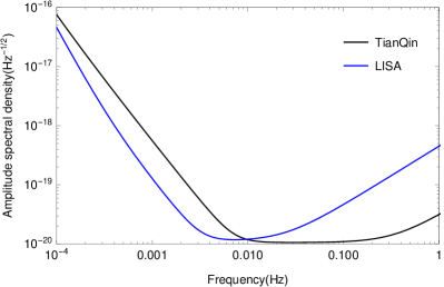
For completeness, we will also consider a second detector, LISA Audley et al. (2017), now adopted by the European Space Agency and due to launch in the early 2030s’. We will consider the joint capability of TianQin and LISA to test the no-hair theorem. For LISA, we will use the sensitivity curve given in Robson et al. (2019), and the frequency bound of is no longer the case. An illustration of sensitivity curve of TianQin and LISA is given in Fig:1.
II.3 Statistical methods
For a pair of frequency domain signals and , one can define the inner product Finn (1992).
| (11) |
where the factor of 2 comes from the single side integration of the frequency. In order to prevent spurious power arising from the Fourier transformation, is taken to be half of the oscillation frequency for mode, and is taken to be twice of the oscillation frequency for mode, which follows the choice of Gossan et al. (2012). While our results are sensisitve to the choice of , choosing this lower limit of integration is analogous to setting a starting frequency for the ringdown, which is known to be a delicate problemBaibhav et al. (2018); Isi et al. (2019). Our results are insensitive to the choice of , provided that it is taken to be sufficiently large.
Signals in the frequency domain are obtained from the time domain signals through the Fourier transformation:
| (12) |
and the SNR for a GW signal is simply defined as
| (13) |
If the sources are isotropically distributed, one can get rid of the SNR dependence on the sky position by performing an angular average. The sky averaged SNR can be given by Eq. (13) with to be the signal before detector response.
In the case of large SNR signals, the uncertainty in the parameter estimation is given by
| (14) |
where are the waveform parameters to be estimated, denotes the expectation value, and is the inverse of the Fisher information matrix Finn (1992); Cutler and Flanagan (1994); Vallisneri (2008),
| (15) |
For the single ringdown signal, we deal with a 16-dimensional parameter space
| (16) |
Under the assumption that the no-hair theorem violating parameters and are independent of the source, more stringent constrains can be reached by combining multiple detections. The incoherent superposition of multiple signals can be expressed as
| (17) |
Each single signal can be regarded as independent,
| (18) |
with denoting the parameters related to the source . In this case, the full parameter space is
| (19) |
III Results
In this section, we present preliminary results on TianQin-based projected tests of the no-hair theorem with ringdown signals. In III.1, we discuss the case of individual detections by TianQin alone, and by TianQin and LISA. In III.2, we consider the case when all detected events are combined together, considering different possible detector configurations.
III.1 Single detections
We start here by considering individual detections. For simplicity, we consider a mildly inclined binary with , and without loss of generality we set and .
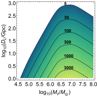
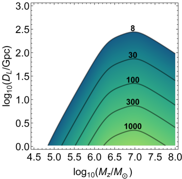
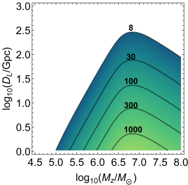
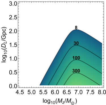
Contour plots of the SNR of the four strongest QNMs as a function of the red-shifted final mass and luminosity distance are given in Fig. 2. One can see that the mode is the strongest, while the and the modes are comparable to one another.

The dependence of the parameter estimation accuracy on the black hole mass is illustrated in Fig. 3. The observed total mass affects the parameter estimation in two ways, i.e. through the GW amplitude and the GW frequencies. For , the amplitude effect dominates and the constraints get worse with smaller mass (since the amplitude scales linearly with the mass). For , the frequency effect dominates, and the constraints get worse with larger mass (because the latter leads to lower GW frequencies, which eventually fall outside the most sensitive frequency band of TianQin).
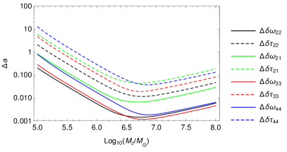
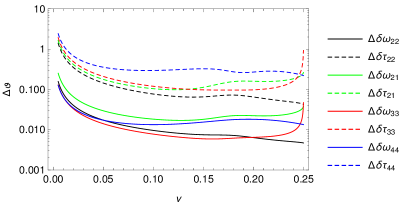
Fig. 4 illustrates the dependence of the parameter estimation accuracy on the symmetric mass ratio of the progenitor binary. The first feature is that the accuracy becomes worse for smaller mass ratios. This is because the radiated energy becomes smaller with smaller symmetric mass ratio, when the total mass is fixed. The second feature is that the constraint on the mode becomes worse as the binary masses become comparable. This is because the amplitude of the mode becomes zero when , as it is obvious from equation (II.1). In that limit, one should use other parameters, such as and , to test the no-hair theorem.
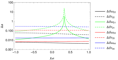
The dependence of the parameter estimation accuracy on the effective spin is plotted in Fig. 5. The effective spin has negligible effect on parameter constraints, except for and . The divergence of and appears because the amplitude of the 21 mode tends to zero when , as shown in equation (II.1)
The dependence of the parameter estimation accuracy on the luminosity distance is shown in Fig. 6. The errors are inversely proportional to . This is because the amplitude of the GW is proportional to , and as a result all components of the covariance matrix are proportional to to .
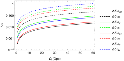
Fig. 7 shows the parameter estimation accuracy as a function of the final spin. The radiated GW frequencies become larger for larger spins, and so is the constraining power.
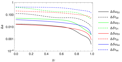
From the above figures, one can see that , and are typically the most constrained parameters. We thus will focus on these parameters in the following.
Since LISA and TianQin should be launched around the same time, we can also consider a joint detection by the two missions. The two detectors are most sensitive at different frequencies, and the frequency of the ringdown signal is inversely proportional to the mass of the remnant. It is therefore interesting to investigate the capabilities of the two instruments (and of the combined observations) as a function of remnant black hole mass.
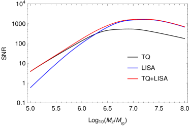
An illustration of the ringdown SNR for TianQin, LISA and a joint detection as a function of the observed final mass is given in Fig. 8. Around , when the SNRs for both detectors are comparable, a joint detection can improve the total SNR by a factor of about 1.4 at best.
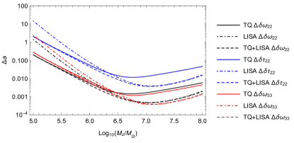
Fig. 9 shows the estimation accuracy of (black), (blue) and (red) estimation accuracy for TianQin (full line), LISA (dot-dash line) and a joint detection (dash line), as a function of the observed final mass. The constraint can be improved by a factor of about 1.4 near with a joint detection.
This nicely shows the complementarity of LISA and TianQin. The former will dominate the measurement for while the latter will provide much better constraints for .
III.2 Combined constrains from all observed events
Massive black hole population models predict that TianQin can detect from tens to few hundreds of massive black hole mergers during its five years operation time Wang et al. (2019); Feng et al. (2019). In this subsection, we study how TianQin and LISA can test the no-hair theorem by combining their massive black hole detections. As a comparison, we will also consider the case for both sigle constellation and a twin constellation of TianQin running for 5 years (labeled as “TQ” and “TQ_tc” respectively), LISA running for 4 years (labeled as “LISA_4y”) and LISA running for 10 years (labeled as “LISA_10y”).
The number and properties of massive black hole mergers that can be detected are largely model dependent. We will use the same three scenarios for the merger history of massive black holes investigated in Klein et al. (2016); Wang et al. (2019) and generated according to the semi-analytic model presented in Barausse (2012) and successively improved in Sesana et al. (2014); Antonini et al. (2015). The three scenarios are referred to as “popIII”, “Q3_d” and “Q3_nod”, corresponding, respectively, to a light seed model Madau and Rees (2001) and to two heavy seed models Bromm and Loeb (2003); Begelman et al. (2006); Lodato and Natarajan (2006) with and without time delays between the mergers of massive black holes and those of their host galaxies. We refer the readers to Barausse (2012); Sesana et al. (2014); Antonini et al. (2015) for a detailed description of these three models.
For each of the detector scenarios, we produce 1000 mock catalogues of observed events from each of the three astrophysical models. Each catalogue consists of all the events that can be detected under the corresponding detector scenario. We assume a detection threshold of 8 for the SNR of total Inspiral-Merger-Ringdown(IMR) signal (), we also assume a detection threshold of 8 for the SNR of total Ringdown stage (). For a given detector scenario, the expected IMR detection number and Ringdown detection number are obtained by averaging over the 1000 mock catalogues.
Using the criterion provided in Berti et al. (2016, 2007) (see in particular Eqs. 2 and 3 of Berti et al. (2016) for readily usable formulae), , where is the SNR for generalized likelihood ratio test, requiring that the SNR in the ringdown alone should be sufficient for the first subleading mode to be resolvable from the leading one, one can calculate the number of events that can be used to test the no-hair theorem. We call these events the “testing events”. For a given detector scenario, the expected number of testing events is also obtained by averaging over the mock catalogues.
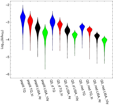
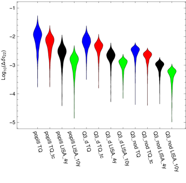
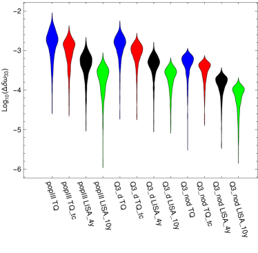
The results on expected constraints on the no-hair theorem violating parameters , and are presented in figure 10, 11 and 12 respectively, and summarized in Table 2. Once fixed the detector and the MBH scenario, each of the 1000 mock catalogs will result in a different number of testing events with different properties, and thus in a different constraint on the parameters. The distribution of these combined constraints over the 1000 mock catalogs is what is shown by means of ’violin plots’ in the three figures. Conversely, the table reports the mean value of the constraints over the 1000 realizations, together with the standard deviation.
We first notice that GW detectors are more sensitive to deviations in characteristic frequencies (, and ) rather than damping time . The former being generally constrained about five time better than the latter. Constraints also strongly depend on the assumed MBH population model. Despite resulting in a comparable number of testing events, the Q3_d model provides constraints that are 2-to-3 times tighter than the popIII one. This is because GW sources are generally more massive in the Q3_d model, and the ringdown is detected for almost all the events at high SNR, which is not the case for the popIII model. The even stronger constraints provided by the Q3_nod models are due to the larger number of testing events. Note, however, that compared to the Q3_nod model the improvement does not scale with , as one would naively expect. This is because in the Q3_d model, the MBH binary dynamics is taken into account, resulting in long merger timescales that push the distribution of observed systems at lower redshift compared to the Q3_nod model. Therefore, there are less events available for testing purposes, but they have larger SNR on average. Finally, LISA generally provides a factor 3-to-5 better constraints then TQ on all parameters. Again, this is partly due to the larger number of detected systems, but also by the fact that sources detected by LISA have typically higher SNR than those seen by TQ (cf figure 9). Focusing on TQ, depending on the detector configuration and MBH population model, the decay parameter can be constrained to 0.2% to 1.5% accuracy; these numbers become a factor of better for the frequency parameters (, and ) that can both be constrained within 0.03% to 0.3%.
| Cases | ||||||
| popIII TQ | 51.7 | 16.5 | 12.7 | |||
| popIII TQ_tc | 104.0 | 31.4 | 24.3 | |||
| popIII LISA_4y | 118.5 | 28.9 | 23.0 | |||
| popIII LISA_10y | 296.6 | 72.9 | 58.5 | |||
| Q3_d TQ | 17.7 | 17.2 | 15.1 | |||
| Q3_d TQ_tc | 35.7 | 34.3 | 29.4 | |||
| Q3_d LISA_4y | 29.7 | 28.8 | 24.3 | |||
| Q3_d LISA_10y | 75.5 | 73.6 | 62.0 | |||
| Q3_nod TQ | 274.9 | 247.5 | 162.1 | |||
| Q3_nod TQ_tc | 535.4 | 486.2 | 317.8 | |||
| Q3_nod LISA_4y | 441.8 | 399.7 | 261.4 | |||
| Q3_nod LISA_10y | 1102.8 | 997.8 | 652.1 |
IV Summary and future work
In this paper, we have studied TianQin’s capability to test the no-hair theorem.
We have modeled the waveform of the ringdown signal from the merger of a massive black hole binary, by including the four strongest QNMs of the remnant Kerr black hole. We then used a set of phenomenological parameters modifying the frequencies and the damping times of the QNMs to parametrize the effect of a no-hair theorem violation. We further assumed that the no-hair theorem violating parameters are independent of the other source parameters.
We have used the Fisher information matrix method to study how these parameters are constrained by a single detection of a massive black hole merger by TianQin. We have studied how the constraints on the no-hair theorem violating parameters vary with the observed mass, luminosity distance, final spin, symmetric mass ratio and effective spin of the source.
We have found that , and are the best constrained parameters in the majority of cases. For a single detection, we find that TianQin and LISA provide constraints on those three parameters in different mass ranges: although LISA can extract more information from binaries with M⊙, TianQin is better suited to test no-hair theorem using binaries with M⊙. Joint detections with TianQin and LISA will further improve no-hair theorem tests for binaries of about M⊙, where the performance of the two detectors is comparable. By combining constraints from all the events expected throughout the lifetime of TianQin, , and can be constrained to within , and respectively, depending on the massive black hole population model (see Table 2).
For completeness, we have also considered other detector scenarios, including a twin set of TianQin constellations running for 5 years, and LISA running for 4 years or 10 years. Running a twin set of TianQin trivially improves the constrains by about . LISA, on the other hand, can detect more massive binaries at higher SNR, thus offering the possibility of detecting smaller deviations from the no-hair theorem. Constraints on range between and depending on the massive black hole population model and on the duration of the LISA mission (cf. Table 2).
We note that the present work can be improved in many directions, for example by including the effect of eccentricity of the progenitor binary, by considering more than four QNMs and other GW polarizations in the ringdown signal, and by using more robust parameter estimation methods than the Fisher information matrix. One should also consider how to relate the phenomenological parameters used in this paper to the parameters of a specific theory of gravity which predicting violations of the no-hair theorem. We will provide an explicit example of this latter point in Bao et al. (2019), for the special case of Scalar-Tensor-Vector Gravity.
Acknowledgements.
The authors thank Shun-Jia Huang, Peng-Cheng Li, Xian-Ji Ye,Yi-Fan Wang and John Veitch for useful discussion. We also thank to Gregorio Carullo for kind comments and suggestions. This work has been supported by the Natural Science Foundation of China (Grant Nos. 11805286, 11703098, 91636111, 11690022, 11475064) and by the European Union’s Horizon 2020 research and innovation program under the Marie Sklodowska-Curie grant agreement No 690904. This project has received funding (to E. Barausse) from the European Research Council (ERC) under the European Union s Horizon 2020 research and innovation programme (grant agreement no. GRAMS-815673; project title “GRavity from Astrophysical to Microscopic Scales”). AS is supported by the Royal Society.References
- Abbott et al. (2016a) B. P. Abbott et al. (Virgo, LIGO Scientific), Phys. Rev. Lett. 116, 061102 (2016a), arXiv:1602.03837 [gr-qc] .
- Abbott et al. (2016b) B. P. Abbott et al. (Virgo, LIGO Scientific), Phys. Rev. Lett. 116, 241103 (2016b), arXiv:1606.04855 [gr-qc] .
- Abbott et al. (2017a) B. P. Abbott et al. (Virgo, LIGO Scientific), Astrophys. J. 851, L35 (2017a), arXiv:1711.05578 [astro-ph.HE] .
- Abbott et al. (2017b) B. P. Abbott et al. (Virgo, LIGO Scientific), Phys. Rev. Lett. 119, 141101 (2017b), arXiv:1709.09660 [gr-qc] .
- Abbott et al. (2017c) B. P. Abbott et al. (VIRGO, LIGO Scientific), Phys. Rev. Lett. 118, 221101 (2017c), [Erratum: Phys. Rev. Lett.121,no.12,129901(2018)], arXiv:1706.01812 [gr-qc] .
- Abbott et al. (2016c) B. P. Abbott et al. (Virgo, LIGO Scientific), Phys. Rev. X6, 041015 (2016c), [Erratum: Phys. Rev.X8,no.3,039903(2018)], arXiv:1606.04856 [gr-qc] .
- Abbott et al. (2017d) B. Abbott et al. (Virgo, LIGO Scientific), Phys. Rev. Lett. 119, 161101 (2017d), arXiv:1710.05832 [gr-qc] .
- Abbott et al. (2016d) B. P. Abbott et al. (Virgo, LIGO Scientific), Phys. Rev. Lett. 116, 221101 (2016d), [Erratum: Phys. Rev. Lett.121,no.12,129902(2018)], arXiv:1602.03841 [gr-qc] .
- Berti et al. (2018a) E. Berti, K. Yagi, and N. Yunes, Gen. Rel. Grav. 50, 46 (2018a), arXiv:1801.03208 [gr-qc] .
- Berti et al. (2018b) E. Berti, K. Yagi, H. Yang, and N. Yunes, Gen. Rel. Grav. 50, 49 (2018b), arXiv:1801.03587 [gr-qc] .
- Alexander and Yunes (2018) S. H. Alexander and N. Yunes, Phys. Rev. D97, 064033 (2018), arXiv:1712.01853 [gr-qc] .
- Chamberlain and Yunes (2017) K. Chamberlain and N. Yunes, Phys. Rev. D96, 084039 (2017), arXiv:1704.08268 [gr-qc] .
- Yunes et al. (2016) N. Yunes, K. Yagi, and F. Pretorius, Phys. Rev. D94, 084002 (2016), arXiv:1603.08955 [gr-qc] .
- Barausse et al. (2016) E. Barausse, N. Yunes, and K. Chamberlain, Phys. Rev. Lett. 116, 241104 (2016), arXiv:1603.04075 [gr-qc] .
- Chatziioannou et al. (2015) K. Chatziioannou, K. Yagi, A. Klein, N. Cornish, and N. Yunes, Phys. Rev. D92, 104008 (2015), arXiv:1508.02062 [gr-qc] .
- Israel (1967) W. Israel, Phys. Rev. 164, 1776 (1967).
- Israel (1968) W. Israel, Commun. Math. Phys. 8, 245 (1968).
- Carter (1971) B. Carter, Phys. Rev. Lett. 26, 331 (1971).
- Gibbons (1975) G. W. Gibbons, Commun. Math. Phys. 44, 245 (1975).
- Hanni (1982) R. Hanni, Physical Review D 25, 2509 (1982).
- Goldreich and Julian (1969) P. Goldreich and W. H. Julian, Astrophys. J. 157, 869 (1969).
- Ruderman and Sutherland (1975) M. A. Ruderman and P. G. Sutherland, Astrophys. J. 196, 51 (1975).
- Blandford and Znajek (1977) R. D. Blandford and R. L. Znajek, Mon. Not. Roy. Astron. Soc. 179, 433 (1977).
- Barausse et al. (2014) E. Barausse, V. Cardoso, and P. Pani, Phys. Rev. D89, 104059 (2014), arXiv:1404.7149 [gr-qc] .
- Dreyer et al. (2004) O. Dreyer, B. J. Kelly, B. Krishnan, L. S. Finn, D. Garrison, and R. Lopez-Aleman, Class. Quant. Grav. 21, 787 (2004), arXiv:gr-qc/0309007 [gr-qc] .
- Berti et al. (2006) E. Berti, V. Cardoso, and C. M. Will, Phys. Rev. D73, 064030 (2006), arXiv:gr-qc/0512160 [gr-qc] .
- Berti et al. (2007) E. Berti, J. Cardoso, V. Cardoso, and M. Cavaglia, Phys. Rev. D76, 104044 (2007), arXiv:0707.1202 [gr-qc] .
- Yang et al. (2017) H. Yang, K. Yagi, J. Blackman, L. Lehner, V. Paschalidis, F. Pretorius, and N. Yunes, Phys. Rev. Lett. 118, 161101 (2017), arXiv:1701.05808 [gr-qc] .
- Yang et al. (2018) H. Yang, V. Paschalidis, K. Yagi, L. Lehner, F. Pretorius, and N. Yunes, Phys. Rev. D97, 024049 (2018), arXiv:1707.00207 [gr-qc] .
- Cunha et al. (2017) P. V. P. Cunha, E. Berti, and C. A. R. Herdeiro, Phys. Rev. Lett. 119, 251102 (2017), arXiv:1708.04211 [gr-qc] .
- Barack et al. (2018) L. Barack et al., (2018), arXiv:1806.05195 [gr-qc] .
- Glampedakis et al. (2017) K. Glampedakis, G. Pappas, H. O. Silva, and E. Berti, Phys. Rev. D96, 064054 (2017), arXiv:1706.07658 [gr-qc] .
- Berti et al. (2016) E. Berti, A. Sesana, E. Barausse, V. Cardoso, and K. Belczynski, Phys. Rev. Lett. 117, 101102 (2016), arXiv:1605.09286 [gr-qc] .
- Detweiler (1980) S. L. Detweiler, Astrophys. J. 239, 292 (1980).
- Kamaretsos et al. (2012a) I. Kamaretsos, M. Hannam, S. Husa, and B. S. Sathyaprakash, Phys. Rev. D85, 024018 (2012a), arXiv:1107.0854 [gr-qc] .
- Kamaretsos et al. (2012b) I. Kamaretsos, M. Hannam, and B. Sathyaprakash, Phys. Rev. Lett. 109, 141102 (2012b), arXiv:1207.0399 [gr-qc] .
- Gossan et al. (2012) S. Gossan, J. Veitch, and B. S. Sathyaprakash, Phys. Rev. D85, 124056 (2012), arXiv:1111.5819 [gr-qc] .
- Amaro-Seoane et al. (2012) P. Amaro-Seoane et al., Class. Quant. Grav. 29, 124016 (2012), arXiv:1202.0839 [gr-qc] .
- Punturo et al. (2010) M. Punturo et al., Proceedings, 14th Workshop on Gravitational wave data analysis (GWDAW-14): Rome, Italy, January 26-29, 2010, Class. Quant. Grav. 27, 194002 (2010).
- Abbott et al. (2018) B. P. Abbott et al. (LIGO Scientific, Virgo), (2018), arXiv:1811.12907 [astro-ph.HE] .
- Carullo et al. (2018) G. Carullo et al., Phys. Rev. D98, 104020 (2018), arXiv:1805.04760 [gr-qc] .
- Carullo et al. (2019) G. Carullo, W. Del Pozzo, and J. Veitch, (2019), arXiv:1902.07527 [gr-qc] .
- Brito et al. (2018) R. Brito, A. Buonanno, and V. Raymond, Phys. Rev. D98, 084038 (2018), arXiv:1805.00293 [gr-qc] .
- Isi et al. (2019) M. Isi, M. Giesler, W. M. Farr, M. A. Scheel, and S. A. Teukolsky, (2019), arXiv:1905.00869 [gr-qc] .
- Luo et al. (2016) J. Luo et al. (TianQin), Class. Quant. Grav. 33, 035010 (2016), arXiv:1512.02076 [astro-ph.IM] .
- Wang et al. (2019) H.-T. Wang et al., (2019), arXiv:1902.04423 [astro-ph.HE] .
- Feng et al. (2019) W.-F. Feng, H.-T. Wang, X.-C. Hu, Y.-M. Hu, and Y. Wang, (2019), arXiv:1901.02159 [astro-ph.IM] .
- Hu et al. (2017) Y.-M. Hu, J. Mei, and J. Luo, Natl. Sci. Rev. 4, 683 (2017).
- Audley et al. (2017) H. Audley et al. (LISA), (2017), arXiv:1702.00786 [astro-ph.IM] .
- Chandrasekhar (1984) S. Chandrasekhar, Proceedings, 10th International Conference on General Relativity and Gravitation: Padua, Italy, July 4-9, 1983, Fundam. Theor. Phys. 9, 5 (1984).
- Chandrasekhar and Detweiler (1975) S. Chandrasekhar and S. L. Detweiler, Proc. Roy. Soc. Lond. A344, 441 (1975).
- Leaver (1985) E. W. Leaver, Proc. Roy. Soc. Lond. A402, 285 (1985).
- Onozawa (1997) H. Onozawa, Phys. Rev. D55, 3593 (1997), arXiv:gr-qc/9610048 [gr-qc] .
- Berti et al. (2003) E. Berti, V. Cardoso, K. D. Kokkotas, and H. Onozawa, Phys. Rev. D68, 124018 (2003), arXiv:hep-th/0307013 [hep-th] .
- Berti and Kokkotas (2005) E. Berti and K. D. Kokkotas, Phys. Rev. D71, 124008 (2005), arXiv:gr-qc/0502065 [gr-qc] .
- Kokkotas (1993) K. D. Kokkotas, Nuovo Cim. B108, 991 (1993).
- Meidam et al. (2014) J. Meidam, M. Agathos, C. Van Den Broeck, J. Veitch, and B. S. Sathyaprakash, Phys. Rev. D90, 064009 (2014), arXiv:1406.3201 [gr-qc] .
- London et al. (2014) L. London, D. Shoemaker, and J. Healy, Phys. Rev. D90, 124032 (2014), [Erratum: Phys. Rev.D94,no.6,069902(2016)], arXiv:1404.3197 [gr-qc] .
- London (2018) L. T. London, (2018), arXiv:1801.08208 [gr-qc] .
- Husa et al. (2016) S. Husa, S. Khan, M. Hannam, M. P rrer, F. Ohme, X. Jim nez Forteza, and A. Boh , Phys. Rev. D93, 044006 (2016), arXiv:1508.07250 [gr-qc] .
- Hofmann et al. (2016) F. Hofmann, E. Barausse, and L. Rezzolla, Astrophys. J. 825, L19 (2016), arXiv:1605.01938 [gr-qc] .
- Barausse et al. (2012) E. Barausse, V. Morozova, and L. Rezzolla, Astrophys. J. 758, 63 (2012), [Erratum: Astrophys. J.786,76(2014)], arXiv:1206.3803 [gr-qc] .
- Li et al. (2012) T. G. F. Li, W. Del Pozzo, S. Vitale, C. Van Den Broeck, M. Agathos, J. Veitch, K. Grover, T. Sidery, R. Sturani, and A. Vecchio, Phys. Rev. D85, 082003 (2012), arXiv:1110.0530 [gr-qc] .
- Hu et al. (2018) X.-C. Hu, X.-H. Li, Y. Wang, W.-F. Feng, M.-Y. Zhou, Y.-M. Hu, S.-C. Hu, J.-W. Mei, and C.-G. Shao, Class. Quant. Grav. 35, 095008 (2018), arXiv:1803.03368 [gr-qc] .
- Robson et al. (2019) T. Robson, N. Cornish, and C. Liu, Class. Quant. Grav. 36, 105011 (2019), arXiv:1803.01944 [astro-ph.HE] .
- Finn (1992) L. S. Finn, Phys. Rev. D46, 5236 (1992), arXiv:gr-qc/9209010 [gr-qc] .
- Baibhav et al. (2018) V. Baibhav, E. Berti, V. Cardoso, and G. Khanna, Phys. Rev. D97, 044048 (2018), arXiv:1710.02156 [gr-qc] .
- Cutler and Flanagan (1994) C. Cutler and E. E. Flanagan, Phys. Rev. D49, 2658 (1994), arXiv:gr-qc/9402014 [gr-qc] .
- Vallisneri (2008) M. Vallisneri, Phys. Rev. D77, 042001 (2008), arXiv:gr-qc/0703086 [GR-QC] .
- Klein et al. (2016) A. Klein, E. Barausse, A. Sesana, A. Petiteau, E. Berti, S. Babak, J. Gair, S. Aoudia, I. Hinder, F. Ohme, and B. Wardell, Phys. Rev. D 93, 024003 (2016), arXiv:1511.05581 [gr-qc] .
- Barausse (2012) E. Barausse, Monthly Notices of the Royal Astronomical Society 423, 2533 (2012), arXiv:1201.5888 .
- Sesana et al. (2014) A. Sesana, E. Barausse, M. Dotti, and E. M. Rossi, APJ 794, 104 (2014), arXiv:1402.7088 .
- Antonini et al. (2015) F. Antonini, E. Barausse, and J. Silk, APJ 812, 72 (2015), arXiv:1506.02050 .
- Madau and Rees (2001) P. Madau and M. J. Rees, Astrophys. J. 551, L27 (2001), arXiv:astro-ph/0101223 [astro-ph] .
- Bromm and Loeb (2003) V. Bromm and A. Loeb, Astrophys. J. 596, 34 (2003), arXiv:astro-ph/0212400 [astro-ph] .
- Begelman et al. (2006) M. C. Begelman, M. Volonteri, and M. J. Rees, Mon. Not. Roy. Astron. Soc. 370, 289 (2006), arXiv:astro-ph/0602363 [astro-ph] .
- Lodato and Natarajan (2006) G. Lodato and P. Natarajan, Mon. Not. Roy. Astron. Soc. 371, 1813 (2006), arXiv:astro-ph/0606159 [astro-ph] .
- Bao et al. (2019) J. Bao, C. Shi, H. Wang, J.-d. Zhang, Y. Hu, J. Mei, and J. Luo, (2019), arXiv:1905.11674 [gr-qc] .