Accelerating parameter inference with graphics processing units
Abstract
Gravitational wave Bayesian parameter inference involves repeated comparisons of GW data to generic candidate predictions. Even with algorithmically efficient methods like RIFT or reduced-order quadrature, the time needed to perform these calculations and overall computational cost can be significant compared to the minutes to hours needed to achieve the goals of low-latency multimessenger astronomy. By translating some elements of the RIFT algorithm to operate on graphics processing units (GPU), we demonstrate substantial performance improvements, enabling dramatically reduced overall cost and latency.
I Introduction
The Advanced LIGO Abbott et al. (2015) (The LIGO Scientific Collaboration) and Virgo Accadia and et al (2012) ground-based gravitational wave (GW) detectors have identified several coalescing compact binaries The LIGO Scientific Collaboration and the Virgo Collaboration (2016); Abbott et al. (2016) (The LIGO Scientific Collaboration and the Virgo Collaboration); Abbott et al. (2017); The LIGO Scientific Collaboration et al. (2017a, b, c). The properties of the sources responsible have been inferred via Bayesian comparison of each source with candidate gravitational wave signals The LIGO Scientific Collaboration and the Virgo Collaboration (2016); Abbott et al. (2016) (The LIGO Scientific Collaboration and the Virgo Collaboration); Abbott et al. (2017); The LIGO Scientific Collaboration et al. (2017a, b, c, 2018); Pankow et al. (2015); Lange et al. (2018); Veitch et al. (2015). Many more are expected as observatories reach design sensitivity Abbott et al. (2016). Both to handle the rapid pace of discovery and particularly to enable coordinated multimessenger followup, GW observatories should be able to reconstruct the evidence for a signal being present in the data along with the full source parameters of coalescing binaries as fast as possible The LIGO Scientific Collaboration (2016, 2018). However, particularly when using the best-available waveform models, these calculations can be very costly. For binary neutron stars, detailed inferences even using simplified waveforms take weeks. Even for massive binary black holes, these calculations can take months for costly time-domain effective-one-body models which incorporate the effects of precession.
Several strategies have been developed to reduce the computational cost of parameter estimation Miller et al. (2015); Pankow et al. (2015); Canizares et al. (2015); Smith et al. (2016); Vinciguerra et al. (2017); Zackay et al. (2018). Approaches that have appeared in the literature include generating the approximate solutions more quickly Canizares et al. (2013); Field et al. (2014); Smith et al. (2013); Cannon et al. (2013); Hannam et al. (2014); Lundgren and O’Shaughnessy (2014); interpolating some combination of the waveform or likelihood Blackman et al. (2015); Cannon et al. (2013); Smith et al. (2013); Pürrer (2014); Smith et al. (2014); Pankow et al. (2015); Cole and Gair (2014); Graff et al. (2012); or adopting a sparse representation to reduce the computational cost of data handling Antil et al. (2013); Canizares et al. (2013); Smith et al. (2016); Canizares et al. (2015); Pankow et al. (2015); Cornish (2010); Zackay et al. (2018). Not published but also important are code optimization projects that improve infrastructure, such as better parallelization for lalinference Veitch et al. (2015); LIGO Scientific Collaboration (2018). Some methods, however, achieve rapid turnaround through simplifying approximations. The RIFT/rapidPE strategy described in Pankow et al. (2015); O’Shaughnessy et al. (2017a); Lange et al. (2018); Abbott et al. (2016) (The LIGO Scientific Collaboration and the Virgo Collaboration) eschews these simplifications, performing embarrassingly-parallel inferences even for costly models. However, the method as previously implemented still had a significant net computational cost and noticeable startup time, limiting its diverse potential applications. Previously, B. Miller developed a custom-coded implementation of the relevant likelihood on graphics processing units (GPUs), suggesting substantial performance improvements were possible Miller (2016); Miller and Pankow (2016). The pycbc search codeUsman et al. (2016) and its pycbc-inference extension Biwer et al. (2019) can also make use of several GPU hardware-accelerated operations. In this paper, we describe a variant of the RIFT approach which flexibly translates one of its algorithms to operate on GPUs, and adjusts its workflow to exploit the speed improvements this re-implementation affords.
This paper is organized as follows. In Section II, we review the underlying marginalized likelihood calculations used by RIFT and their updated GPU implementation. In Section III, we quantify the improved performance of our GPU-accelerated code, while assessing operating settings which facilitate increased performance. In Section IV, we describe the performance of the end-to-end pipeline on the synthetic nonspinning signals used in Section III. In Section V, we summarize our results and discuss their potential applications to future GW source and population inference.
II Methods
II.1 Parameter inference with the RIFT likelihood
ILE – a specific algorithm to “Integrate (the Likeilhood) over Extrinsic parameters” – provides a straightforward and efficient mechanism to compare any specific candidate gravitational wave source with real or synthetic data Pankow et al. (2015); Abbott et al. (2016) (The LIGO Scientific Collaboration and the Virgo Collaboration); Lange et al. (2017); O’Shaughnessy et al. (2017a), by marginalizing the likelihood of the data over the seven coordinates characterizing the spacetime coordinates and orientation of the binary relative to the earth. Specifically the likelihood of the data given gaussian noise, relative to gaussian noise, has the form (up to normalization)
| (1) |
where are the predicted response of the kth detector due to a source with parameters (, ) and are the detector data in each instrument k; denotes the combination of redshifted mass and the remaining parameters needed to uniquely specify the binary’s dynamics; represents the seven extrinsic parameters (4 spacetime coordinates for the coalescence event and 3 Euler angles for the binary’s orientation relative to the Earth); and is an inner product implied by the kth detector’s noise power spectrum . In practice we adopt both low- and high- frequency cutoffs so all inner products are modified to
| (2) |
The joint posterior probability of follows from Bayes’ theorem:
| (3) |
where and are priors on the (independent) variables . For each , we evaluate the marginalized likelihood
| (4) |
via direct Monte Carlo integration over almost all parameters , where is uniform in 4-volume and source orientation. For the event time parameter, we marginalize by direct quadrature, for each choice of the remaining Monte Carlo parameters. For the remaining dimensions, to evaluate the likelihood in regions of high importance, we use an adaptive Monte Carlo as described in Pankow et al. (2015).
This marginalized likelihood can be evaluated efficiently by generating the dynamics and outgoing radiation in all possible directions once and for all for fixed , using a spherical harmonic decomposition. Using this cached information effectively, the likelihood can be evaluated as a function of at very low computational cost. A dimensionless, complex gravitational-wave strain
| (5) |
can be expressed in terms of its two fundamental polarizations and . Here, denotes time, and are the polar and azimuthal angles for the direction of gravitational wave propagation away from the source. The complex gravitational-wave strain can be written in terms of spin-weighted spherical harmonics as
| (6) |
where the sum includes all available harmonic modes made available by the model; where is a fiducial reference distance; and where , the luminosity distance to the source, is one of the extrinsic parameters.
Following Pankow et al. (2015), we substitute expression (6) for into the expression for the detector response , where is the arrival time at the th detector (at position ) for a plane wave propagating along Pankow et al. (2015). We then substitute these expressions for into the likelihood function (1) thereby generating Pankow et al. (2015)
| (7) |
where where are the complex-valued detector response functions of the th detector Pankow et al. (2015) and the quantities depend on and the data as
| (8a) | ||||
| (8b) | ||||
| (8c) | ||||
In RIFT, the marginalization in Eq. (4) over extrinsic parameters is performed by evaluating this likelihood on long arrays of extrinsic parameters, including but excluding time. Treating the block of quantities that arise in one sequence of evaluations together, the expressions and can be considered as multi-dimensional arrays. For example, is a matrix indexed over (detectors) and (extrinsic parameters); is a matrix of shape (modes)(extrinsic); and is a one-dimensional array over . By contrast, the are arrays of shape (detectors) (modes)2 are independent of extrinsic parameters. While depends explicitly on time, and varies rapidly on short timescales, varies on the earth’s rotation timescale, so we approximate as time-independent.
At a fixed set of intrinsic parameters , ILE will repeatedly evaluate the time-marginalized likelihood for each candidate Monte Carlo set of extrinsic parameters :
| (9) |
where is a small coincidence window consistent with the candidate event time; here and previously, . Because we treat the parameter asymmetrically when marginalizing over all extrinsic parameters, we likewise organize a multidimensional array representation of to emphasize the special role of time: for each we construct a uniformly-sampled timeseries versus , truncating it to a narrow coincidence window. In effect, we represent by a matrix with shape (detectors)(modes)(extrinsic)(time). In terms of these multidimensional arrays, rewriting sums as matrix operations, the likelihood can be equivalently expressed as
| (10) |
where this symbolic expression employs an implicit index-summation convention such that all naturally paired indices are contracted. The result is an array of shape (time)(extrinsic).
II.2 Accelerated evaluation via efficient multiplication
To accelerate the code, after precomputing the inner products , we simply shift them to the graphics card, then carry out all calculations necessary to implement Eqs. (10, 9) on the GPU. These arrays are only a few kilobytes. We then construct blocks of random extrinsic parameters with the CPU; transfer them to the board; and use on-board code to construct values for . To enable this implementation with portable code, we use cupy Okuta et al. (2017), a drop-in-replacement for equivalent numpy code used for the CPU-based version of ILE. For the most costly part of the calculation – the inner products necessary to evaluate , accounting for distinct time-of-flight-dependent time windows for each interferometer’s data – we use a custom CUDA kernel to perform the necessary matrix multiplication. With these changes alone, the likelihood evaluation is roughly faster on equivalent hardware. After this update, individual likelihood evaluation costs are not the performance- or cost-limiting feature of RIFT-based source parameter inference. Instead, the overhead associated with the adaptive Monte Carlo and with the (CPU-based) inner product evaluations for dominate our computational cost.
II.3 Tradeoff between Monte Carlo integration and accuracy
Each marginalized likelihood evaluation has a relative uncertainty of order , where the number of effective samples increases linearly with the total number of Monte Carlo evaluations performed by ILE. Therefore, to increase (decrease) our accuracy for each likelihood evaluation by a factor of will require a factor more (fewer) iterations. We adopt a fixed threshold on .
We do benefit slightly by re-using the adaptive Monte Carlo integrator for each extrinsic point . Since the integrator has already identified the likely range of sky locations and distances on the first iteration, each subsequent evaluation of the marginalized likelihood can converge marginally more quickly.
III Analysis of marginalized likelihood evaluation cost
We illustrate the code using two synthetic signals: a binary black hole with masses and a binary neutron star with masses and . We perform this analysis on heterogeneous LVC collaboration computing resources described in more detail in the Appendix, to assess our variable performance across architectures. Notably, we investigate the following GPU options: (a) GTX 1050 Ti at LIGO-CIT, available in large numbers; (b) V100, available on selected high-performance machines; (c) and GTX 1050 at LIGO-LHO. Unless otherwise noted in the text, we will discuss code configurations using CPU-only and GPU (b) using sampling and only the modes. In this section, we conservatively report computational cost for parameters which are close to or within the posterior. Because of their consistency with the data, the marginalized likelihood calculations converge the most slowly, as they have the best-determined extrinsic parameters.
III.1 Synthetic source generation and analysis settings
We generate synthetic data for a two-detector LIGO configuration, assuming operation at initial (BBH) or advanced (BNS) design sensitivity. Both signals are generated with SEOBNRv4 effective-one-body waveform approximation Bohé et al. (2017), with a zero-noise data realization. To qualitatively reproduce the noise power spectrum and amplitude of typical binary black hole observations in O1 and O2, the binary black hole signal has source distance , chosen so SNR . Similarly, to qualitatively reproduce the analysis of GW170817, our synthetic binary neutron star is placed away, so the signal amplitude is SNR .
We perform a multi-stage iterative RIFT analysis of these signal with the time-domain SEOBNRv4 (BBH) or TaylorT4 Buonanno et al. (2009)( BNS) approximation, under the simplifying assumption that both objects are point particles with zero spin. For both sources, we adopt the fiducial distance prior , selecting a maximum distance roughly five times larger than the known source distance: 1Gpc for the binary black hole and 500 Mpc for the neutron star. We adopt a uniform prior on the component (redshifted) masses (and, when appropriate, spins ). Unless otherwise noted, all mass quantities described in this work are redshifted masses . For the binary black hole we generate the signal with and analyze the signal with ; for the binary neutron star, we generate the signal with and anayze it with .
III.2 Massive compact binary black holes
Previously, each instance of ILE examined one intrinsic point . The overall cost of this ILE evaluation involved two parts: a startup cost, a setup cost, and a Monte Carlo integration cost. The startup cost is associated with code setup followed by reading, data conditioning, and Fourier-transforming the data. The setup cost arises from waveform generation and the inner products . Finally, the Monte Carlo cost increases with the number of Monte Carlo iterations with and the number of times the sampling prior used in adaptive Monte Carlo is regenerated from the most recent data points, in proportion to their cost. In the standard configuration, the adaptive sampling prior is regenerated every iterations (i.e, ), regenerating a sampling prior in two sky location parameters and distance. The choice of one for each instance of ILE was due to the substantial time , which vastly dominated the overall computational cost. For example, for a typical analysis of a short signal – a typical binary black hole signal with and – this version has cost elements as shown in Table 1, based on the assumption that the MC terminates after iterations using . The marginalized likelihood described above converges incredibly rapidly to a small value if the candidate model is inconsistent with a signal (or the absence thereof) in the data, with only evaluations needed.
| Version | srate | modes | GPU | ||||||
|---|---|---|---|---|---|---|---|---|---|
| Hz | m | sec | sec | sec | sec | sec | use % | ||
| CPU | 16384 | 20 | 2.4 | 540 | 20 | 690 | |||
| 4096 | 20 | 20 | |||||||
| CPU | 16384 | 20 | 1.5 | 680 | 20 | 1060 | |||
| 4096 | 20 | 20 | |||||||
| GPU (a) | 16384 | 20 | 270 | ||||||
| 4096 | 20 | 45 | |||||||
| GPU (b) | 16384 | 20 | 1.8 | 1 | 0.85 | 20 | 28 | 15 | |
| 4096 | 20 | 1 | 0.75 | 20 | 25 | ||||
| GPU (b) | 16384 | 20 | 1 | 4.2 | 20 | 38 | |||
| 4096 | 20 | 1 | 2.5 | 20 | 35 | ||||
| GPU (c) | 16384 | 20 | 6 | 18 | 58 | 160 | |||
| 4096 | 20 | 3.7 | 11 | 58 | 140 |
With the new low-cost evaluations, however, the startup and setup costs now can be comparable or in excess of the total time used to evaluate the marginalized likelihood . In fact, the total time per Monte Carlo evaluation spent in general-purpose overhead will be much larger than the time spent carrying out scientific calculations by evaluating the likelihood. For these reasons, we reorganize the workflow, so each instance of ILE loops over different choices for . Additionally, particularly for massive binary black holes, we investigate two additional performance improvements. First and foremost, we lower the sampling rate, thus lowering the startup cost and particularly setup cost . Previously and out of an abundance of caution, ILE employed a sampling rate for all calculations, but terminated all inner products in Eq. (2) at roughly or less. Reducing the sampling rate by a factor will reduce the cost of all operations with timeseries – they are shorter. Depending on the relative cost of overhead versus array operations, and the cost per evaluation decrease modestly because of this effect. Also following Pankow et al, to insure safe inner products over short data sets in the presence of very narrow spectral lines, we operated on a significantly-padded data buffer and modified the noise power spectrum by truncating the inverse power spectrum to a finite response time. For binary black holes, the degree of padding was significantly in excess of the signal duration. Instead and following lalinference Veitch et al. (2015), we adopt a much shorter inverse spectrum truncation length, a much shorter padding buffer, and a Tukey window applied to the data to remove discontinuities at the start and end of each segment. Reducing the duration of data analyzed by a factor will reduce the cost by a factor . Combining these factors together, the overall computational cost of each marginalized likelihood evaluation is
| (11) |
The first rows in table Table 1 shows our estimated breakdown of these elements of the computational cost, for a typical binary black hole signal with and . Because of the extremely high cost of adaptive overhead, we only adapt in two parameters, corresponding to sky location; and only adapt until a marginalied likelihood evaluation returns significant . As a result, (the number of adaptive stages per likelihood evaluation) scales as and does not increase with the overall number of samples, so the overall evaluation time scales as
| (12) | ||||
| (13) |
where in the latter expression we substitute the usual values of , , and conservtively adopted for problems involving many degrees of freedom (between 6 to 8). We target so that startup and other one-time costs are not a significant contributor to the overall runtime. In this configuration, the run time per marginalized likelihood is around for a binary black hole. Of this , only roughly corresponds to evaluating the likelihood, implying the cost . Likewise, because overhead dominates over array manipulations, an analysis with timeseries requires only marginally more time than the corresponding analysis. Conversely, the overhead of performing the Monte Carlo (including both and ) is a quite substantial contribution to the overall runtime for the best-available hardware.
For low-latency analyses, we need to assess the overall wallclock time needed to perform an analysis, often with a restricted number of available GPU-enabled machines. To complete likelihood evaluations with these resources requires
| (14) |
Typically we target , or roughly the cost per individual marginalized likelihood evaluation. For the binary black hole configuration described above, marginalized likelihood evaluations will complete in about on a cluster of (b), or more realistically 200 minutes on a cluster of (a). This number can be reduced to tens of minutes with a modestly larger GPU pool, or by marginally more conservative convergence thresholds or . This discussion ignores the latency introduced by the gaussian process interpolation stage at the end. We will revisit accelerated GP interpolation in subsequent work.
The ILE likelihood generates waveform dynamics and once per evaluation . Waveform generation can contribute significantly to the time needed to evaluate for extremely costly waveform models which require a significant fraction of . That said, the tests described above used relatively costly waveform generation with allocation requiring at 4kHz and at 16 kHz.
The ILE likelihood involves sums over modes, with the most expensive likelihood and setup operations (involving ) growing linearly with the number of modes used. This increased cost is most apparent in Table 1 when comparing the columns corresponding for GPU (b) between the and rows. The cost of evaluating with 4 modes is roughly twice that of runs with two modes, as expected.
In a heterogeneous computing environment, code performance varies substantially with available resources, as seen by contrasting corresponding results for (a,b,c) in Table 1. For the slowest hardware, the overall runtime will be only a factor few smaller than the corresponding CPU-only runtime.
III.3 Binary neutron stars
| Version | srate | modes | GPU | ||||||
|---|---|---|---|---|---|---|---|---|---|
| Hz | m | sec | sec | sec | sec | sec | use % | ||
| CPU | 16384 | 35 | 26 | 0.14 | 680 | 25 | 590 | ||
| 4096 | 35 | 25 | |||||||
| GPU (a) | 16384 | 35 | |||||||
| 4096 | 35 | 60–450 | |||||||
| GPU (b) | 16384 | 35 | 26 | 0.07 | 2.4 | 35 | 16 | ||
| 4096 | 35 | 11.5 | 0.1 | 2.4 | 24 | ||||
| GPU (c) | 16384 | 35 | 71 | 20 | 38 | 105 | |||
| 4096 | 35 | 28 | 12 | 60 |
Table 2 shows the corresponding performance breakdown for our fiducial binary neutron star, which has signal SNR=32. In this analysis, we have adopted the TaylorT4 model with and all modes as our fiducial analysis template. This source has significantly longer duration and higher amplitude, both of which contribute to slower convergence and longer runtime.
Low-mass compact binaries like binary neutron stars have much longer inspiral times from the same starting frequency of : roughly . Nominally, the manipulation of a corresponding power-of-two duration data () involves more costly Fourier transforms and time integrations than the BBH analysis described above. [An array of of data at corresponds to 32 Mb.] Comparing appearing in Tables 1 and 2, we indeed find our BNS analysis requires a factor of order longer to set up all necessary inner products. Unlike the BBH analysis, the inner product evaluation costs in now dominates the overall evaluation time .
Improved performance arises in part from re-using our adaptive integrator, which (after the first marginalized likelihood evaluation) can exploit tight localization afforded by the many BNS cycles available in band and the high amplitude of our fiducial BNS signal. In some cases, the Monte Carlo integral converges to our target accuracy in of order fewer steps than for BBH. Additionally, particularly for first-stage RIFT grids, the improved performance arises from our choice of initial grid: many points fit poorly and identified as such well before the fiducial Monte Carlo iterations. Both sources of improved performance relative to the BBH analysis are independent of choice of hardware.
For the closed-form post-Newtonian approximation used in the study above, waveform costs are a modest contribution to overall runtime, contributing only 4.1 sec to at 16 kHz. For other approximations not available in closed form, the waveform generation cost for binary neutron star inspirals can be much more substantial, particularly as decreases below the 20Hz used in this study.
While GPU cards have finite memory, the modest size of our underlying data arrays and intemediate data products on-board ensures that we are unlikely to saturate this bound, even for 16 kHz data, unless we investigate significantly lower starting frequencies or employ vastly more angular modes .
IV Performance and validation demonstrations with full pipeline
To better illustrate code performance in realistic settings, we also describe end-to-end analyses with the original and modified code. In a full analysis, many of the initially-proposed evaluation points are either not or marginally consistent with the data. As a result, most marginalized likelihood evaluations in the first iteration proceed extremely rapidly. As the high-cost and low-cost evaluations are generally well-mixed between different instances, the overall time to complete the full first iteration is typically much lower than subsequent iterations. With a well-positioned and sufficiently large initial grid, few follow-on iterations are needed.
IV.1 Binary black hole analysis
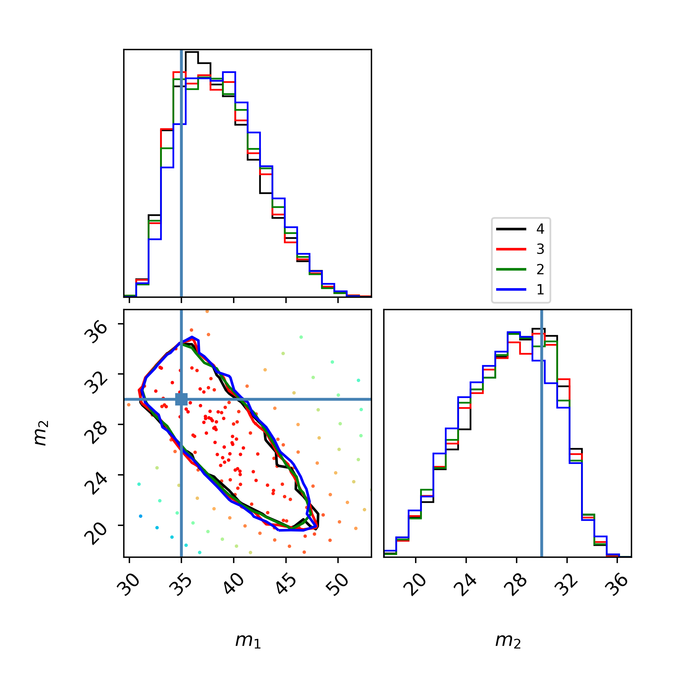

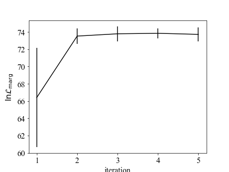
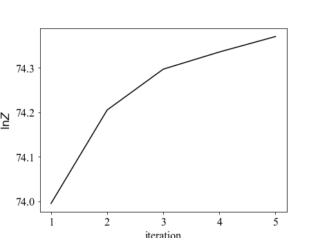
Modest-amplitude short-duration binary black holes empirically constitute the most frequent detection candidates for current ground-based GW observatories The LIGO Scientific Collaboration et al. (2018). Because of their brevity and hence broad posterior, the RIFT code’s interpolation-based method converges rapidly. Combined with the low cost of each iteration, these sources require an exceptionally low committment of resources and can be performed in extremely low latency, as desired. To demonstrate this, we use the GPU-accelerated code with , analyzing data with . We use 100 points in the first iteration, in a very coarse mass grid (i.e., spacing comparable to typical astrophysical mass scales), followed by 20 points in each subsequent iteration. Figure 1 shows our results. The final posterior is already well-explored with the initial gridpoints, and converged by the second iteration. Conversely, on average all iterations required roughly 45 seconds per to evaluate their grid on GPU (a) hardware. This configuration therefore converged within the 30 minutes needed for the first two iterations. We can achieve smaller turnaround time for an otherwise identical analysis by adjusting appropriate to the available hardware. While this low-dimensional problem does not capture all fitting and automation challenges associated with high-dimensional fully precessing binaries, it does capture the low cost and rapid response possible with RIFT.
IV.2 Binary neutron star analysis : Assuming zero spin
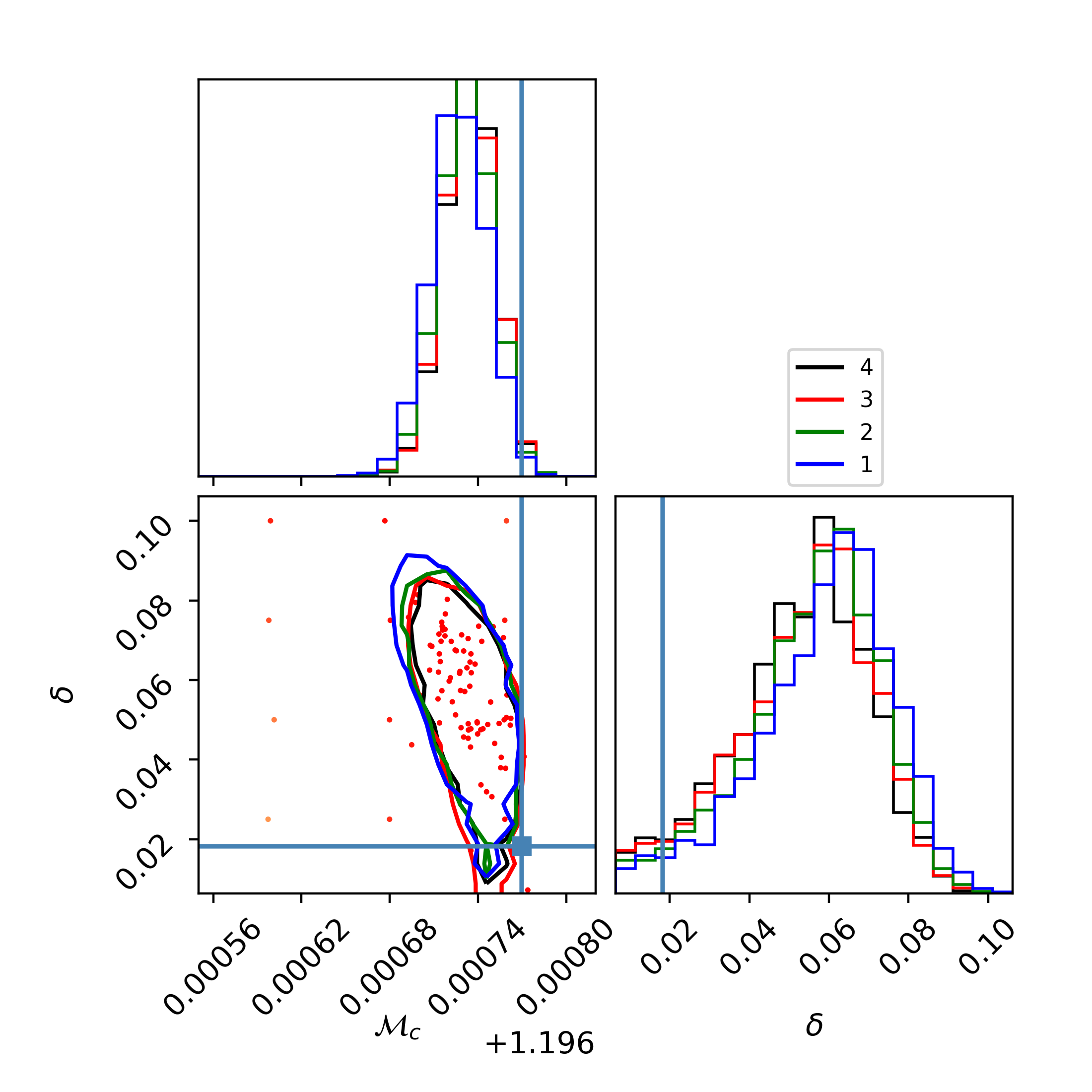
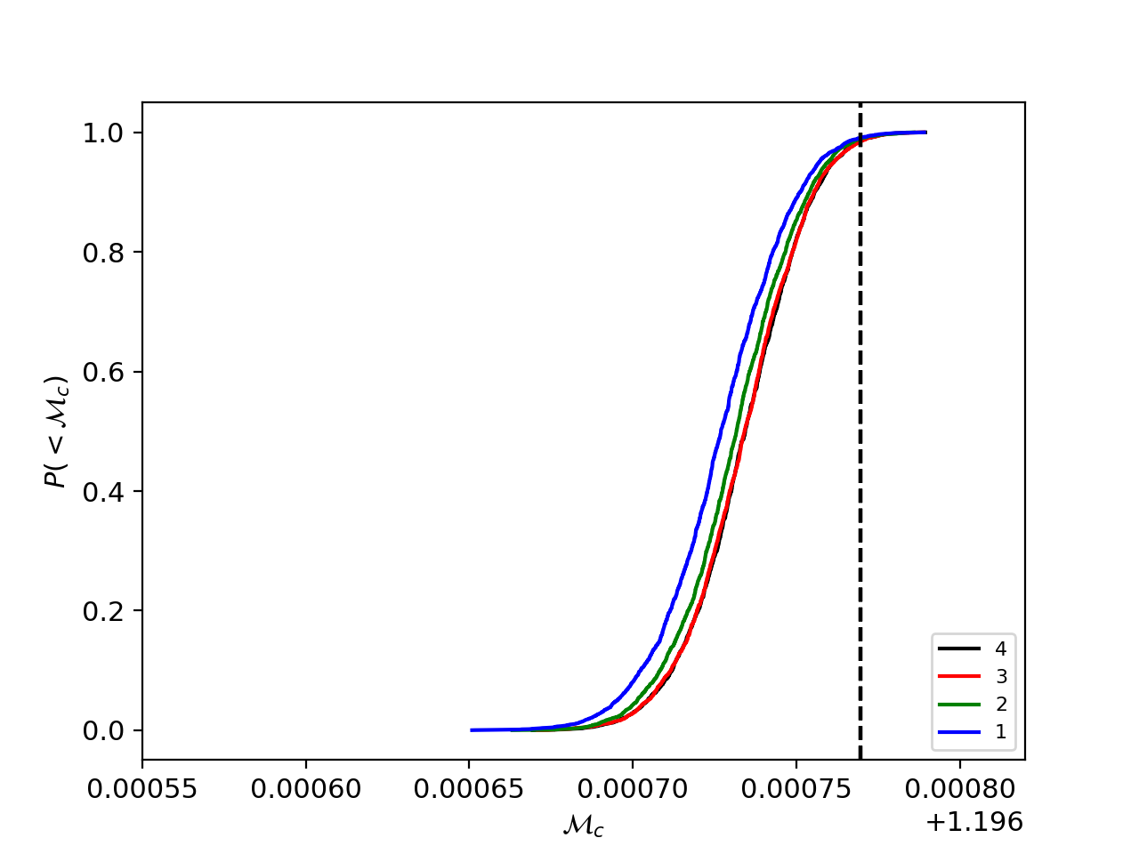

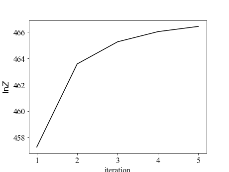
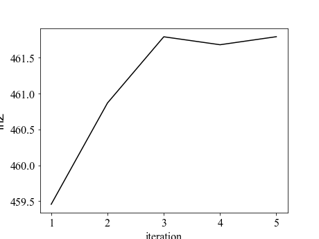
Significant-amplitude binary neutron star mergers are the most important scenario for rapid parameter inference, as low latency can enable multimessenger followup The LIGO Scientific Collaboration et al. (2018). In our second test we compare two workflows, one with the original embarrassingly-parallel RIFT code using and one with the “batched” GPU-accelerated code with , analyzing data with . In this example, we use initial points spread over the two mass dimensions , adding evaluations per iteration. We choose this simple low-dimension, small-size, and slowly-converging configuration to facilitate visualization of the grid, posterior, and convergence. The initial coarse grid covers a region and , insuring the posterior was smaller than our initial coarse grid spacing. The top panels of Figure 2 show posterior distributions derived from the first several RIFT iterations, while the bottom panels show convergence diagnostics. Because our analysis uses a post-Newtonian model to interpret a signal generated with SEOBNRv4, the peak posterior density is slightly offset from the synthetic signal’s parameters
This specific workflow configuration reduces overall core usage by maximizing GPU use per iteration: after the first iteration, only one GPU is active. Specifically, with the updated RIFT workflow used here, with one instance analyzing each 20 evaluations, we use five core+GPU pairs in the first iteration, followed by one core+GPU for remaining iterations. By contrast, with the original CPU-only RIFT code analyzing each in parallel, this process requires roughly 20 core-minutes per , using 100 cores in the first iteration and 20 cores in each subsequent evaluation. Note that because for the GPU is larger than the (hardware-and dependent) speedup factor between the CPU and GPU implementation, the overall wallclock time needed for a end-to-end analysis analysis is larger for the GPU workflow. We can achieve comparable or smaller turnaround time for an otherwise identical analysis by adjusting appropriate to the available hardware.
IV.3 Binary neutron star analysis : Assuming nonprecessing spin
Binary neutron star models with more parameters like spin and tides require correspondingly larger numbers of points in the initial grid and per iteration. Fortunately, the number of observationally significant and accessible dimensions is often substantially less than the prior dimensionality. In practice,we use roughly more points per iteration for precessing massive BBH systems () or for spinning binary neutron stars with tides (). As a result, we can still achieve relatively rapid turnaround on a high-dimensional binary neutron star analysis even in resource-constrained environments.
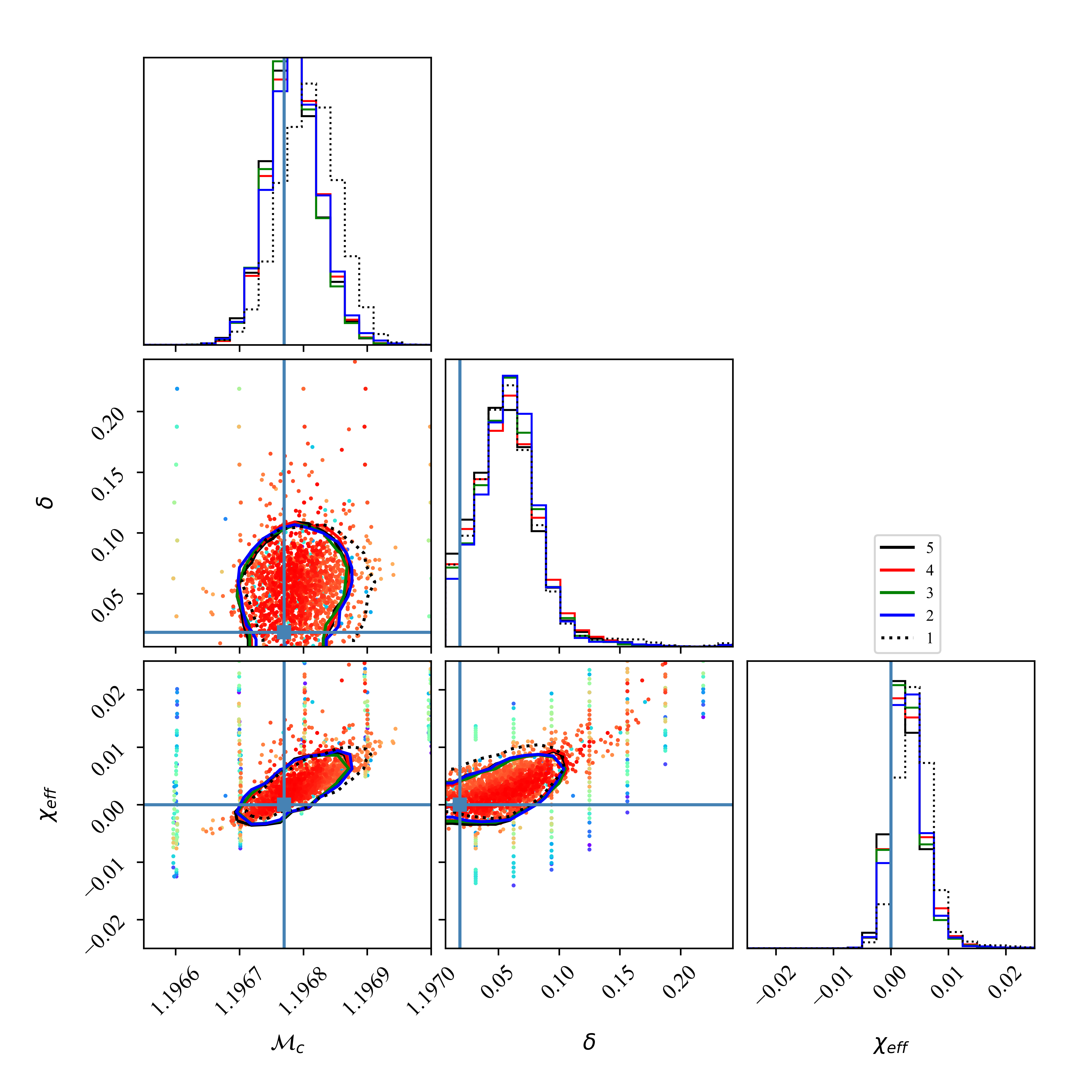
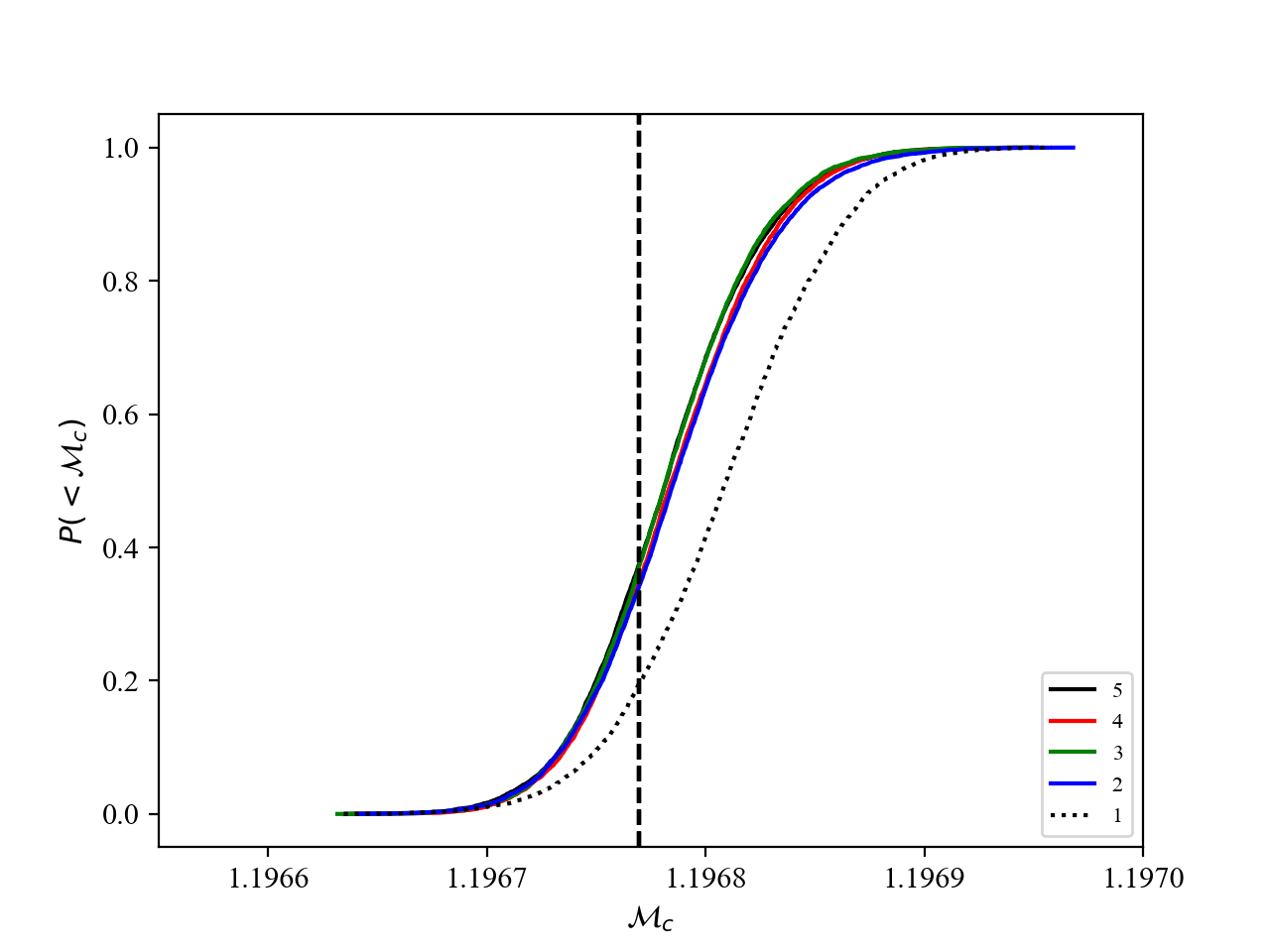
As a concrete demonstration of a realistic modest-latency analysis using the GPU-accelerated code, we reanalyze our fiducial binary neutron star signal, accounting for the possibility of nonzero (aligned) neutron star spins. Our initial grid consists of 5000 points, spread approximately uniformly across a 4-dimensional hypercube , and . Subsequent iterations use 500 random draws from the estimated posterior samples produced from the previous iteration. Because our fiducial post-Newtonian model (TaylorT4) as implemented in lalsuiteLIGO Scientific Collaboration (2018) does not include spin, we employ both the SEOBNRv4_ROM and SpinTaylorT4 waveform approximations for nonprecessing binaries, omitting higher-order modes. For SEOBNRv4_ROM, we use 48 GPU (c) enabled nodes; for SpinTaylorT4, we use 100 GPU (a) nodes. Figure 3 shows our results.
Due to our self-imposed resource constraints on and the number of GPUs, the first iteration is resource-limited and requires of order to times as long as the first iteration of the zero-spin BNS analysis described above. Each marginalized likelihood evaluation in the first iteration (as well as subsequent iterations) requires roughly 60 seconds for both SpinTaylorT4 and SEOBNRv4ROM, on average. Subsequent marginalized likelihood iterations are not resource-limited and complete in roughly 35 minutes, depending on hardware. As previously, we can achieve comparable or smaller turnaround time for an otherwise identical analysis by adjusting appropriate to the available hardware.

V Conclusions
We have demonstrated that the marginalized likelihood appearing in the RIFT/rapidPE parameter inference calculation can be evaluated at fixed in tens of seconds on average for both binary black holes and binary neutron stars. This performance improvement could enable very low latency source parameter inference for compact binaries, which can be of use for targeting multimessenger followup observations via sky localization and precise source characterization. This prospect is particularly interesting because RIFT can often achieve this performance using computationally costly models for binary merger with rich physics like higher modes or eccentricity, as the waveform generation cost does not usually limit code performance.
In addition to producing results rapidly, RIFT results can be produced with a noticably smaller overall resource footprint than loosely similar LI analyses, even without tuning to optimize RIFT pipeline settings. As a concrete and non-optimized example, for all five of the iterations of the spinning binary neutron star parameter inference with SEOBNRv4_ROM from described in this work, our RIFT analysis expended roughly 14 core-days. By contrast, a TaylorF2 analysis of GW170817 with LI in MCMC mode starting from required 228 core-days. For precessing binary black holes using SEOBNRv3, the improvement is equally substantial: 10 core-days for a 10-iteration investigation of a synthetic GW150914-like source with RIFT, versus 291 core-days for a LI analysis of GW170729. We defer detailed relative benchmarking using comparably-converged parameter inference to future work.
The overall code performance and thus latency can be further decreased substantially, notably by converting the Monte Carlo random number generation and inner products to GPU-based operations. In such a configuration, the marginalized likelihood code would perform almost all calculations (except waveform generation) on a GPU, with minimal communication off the board. This configuration should further reduce the average time needed to compute for both binary black holes (which are Monte Carlo limited) and binary neutron stars (which are inner-product limited). We anticipate a further factor of roughly 10 reduction in overall evaluation time can be achieved soon. At that level of performance, a single 8-GPU machine with contemporary hardware could perform parameter inference less than 10 minutes. Since binary compact objects intersect our past light cone only once every roughly 15 minutes, accounting for all past history, such a configuration would be able to address low-latency parameter inference for the duration of 2nd-generation ground-based observing. Alternatively, if larger resource pools are available in low latency, both the original and now GPU-accelerated RIFT can perform extremely rapid parameter inference if large iterations are performed completely in parallel (i.e., ).
By allowing models with higher-order modes to be used in low latency, our code can exploit the tighter constraints which higher modes can enable on the properties of low-mass binaries with suitable amplitudes and orientations. These tighter constraints could better inform low-latency source classification and hence multimessenger followup observations of compact binary mergers.
Beyond low-latency multimessenger astronomy, rapid parameter inference enables new applications. For example, every parameter inference provide evidence for a signal being present in the data; with rapid parameter inference, this evidence could be used as (the last stage in a hierarchical pipeline for) a detection statistic Smith and Thrane (2018). This approach can identify individual events and even a population. Alternatively and in many ways equivalently, one can identify a population of GW sources without assuming any one is real, by applying parameter inference to more candidate events and self-consistently separating foreground and background Farr et al. (2015); Gaebel et al. (2019).
When suitable surrogate models are available, the overall code performance and thus latency could be yet again further reduced by eliminating the iteration and fitting stages entirely, performing one Monte Carlo at once O’Shaughnessy et al. (2017b). This approach exploits a linear representation of via basis functions, to enable rapid likelihood evaluation as a function of both extrinsic parameters and . Though not necessarily or compactly available for all surrogate models, particularly for the small basis sizes necessary to fit onboard GPUs, this approach could enable exceedingly low latency at small computational cost. This alternative architecture would be exceptionally well-suited to the alternative applications of low-latency PE described above.
The use of cupy enables our code to be highly portable across architectures and heterogeneous GPU environments, while transitioning smoothly between GPU and CPU mode. The techniques we used here will be transported to other Bayesian inference modeling codes used to interpret GW observations Wysocki et al. (2018); Wysocki and O’Shaughnessy (2018).
In this work, we have focused exclusively on profiling a simplified pipeline to produce posterior distributions for detector-frame intrinsic parameters. The code also produces reliable extrinsic parameter distributions Pankow et al. (2015). With some postprocessing, this pipeline provides joint posterior distributions for all intrinsic and extrinsic parameter distributions together; examples of these distributions have been published elsewhere The LIGO Scientific Collaboration et al. (2018). Presently, rather than harvest extrinsic information from every iteration, we harvest joint intrinsic and extrinsic information with a single final iteration, which we will implement shortly in our production pipeline.
Acknowledgements.
We thank our anonymous referee for helpful feedback. DW thanks the RIT COS and CCRG for support, and NSF-1707965. JL is supported by NSF PHY-1707965. RO’S is supported by NSF PHY-1707965 and PHY-1607520. Y-LLF was supported in part by BNL LDRD projects No. 17-029 and No. 19-002, and New York State Urban Development Corporation, d/b/a Empire State Development, under contract No. AA289. We thank the Computational Science Initiative at BNL for hosting GPU Hackathon 2018, during which a part of this work was conducted. We also thank Jeff Layton at NVIDIA for bringing CuPy to our attention.Appendix A Properties of resources used
LIGO-CIT worker nodes, denoted by (a) in the text, are principally S6 nodes with 2-CPU core Opteron 2.3 GHz machines with 16 Gb of RAM, with GTX 1050 Ti cards with 4 Gb of RAM. For LIGO-CIT, profiling reports reflect performance averaged over the whole cluster and hence lacks the detailed reporting produced for the other configurations. LIGO-LHO worker nodes with GPUs, denoted by (c) in the text, are a heterogeneous configuration mostly consisting of (a). Unlike profiling at LIGO-CIT, the profiling for LIGO-LHO reflects controlled tests on a single node. The V100 machine (ldas-pcdev13, denoted by (b) in the text) is a 24-core ES-2650 v4 machine with 4 GPUs, only one of which is active in our tests: Tesla V100 with 16 Gb of RAM. All non-GPU profiling was also performed on this machine.
References
- Abbott et al. (2015) (The LIGO Scientific Collaboration) B. Abbott et al. (The LIGO Scientific Collaboration), Class. Quant. Grav. 32, 074001 (2015), eprint 1411.4547.
- Accadia and et al (2012) T. Accadia and et al, Journal of Instrumentation 7, P03012 (2012), URL http://iopscience.iop.org/1748-0221/7/03/P03012.
- The LIGO Scientific Collaboration and the Virgo Collaboration (2016) The LIGO Scientific Collaboration and the Virgo Collaboration, Phys. Rev. Lett 16, 061102 (2016).
- Abbott et al. (2017) B. P. Abbott, R. Abbott, T. D. Abbott, F. Acernese, K. Ackley, C. Adams, T. Adams, P. Addesso, R. X. Adhikari, V. B. Adya, et al., Physical Review Letters 118, 221101 (2017), eprint 1706.01812.
- Abbott et al. (2016) (The LIGO Scientific Collaboration and the Virgo Collaboration) B. Abbott et al. (The LIGO Scientific Collaboration and the Virgo Collaboration), Phys. Rev. X 6, 041015 (2016), eprint 1606.04856, URL https://journals.aps.org/prx/abstract/10.1103/PhysRevX.6.041015.
- The LIGO Scientific Collaboration et al. (2017a) The LIGO Scientific Collaboration, the Virgo Collaboration, B. P. Abbott, R. Abbott, T. D. Abbott, F. Acernese, K. Ackley, C. Adams, T. Adams, P. Addesso, et al., Phys. Rev. Lett 119, 141101 (2017a), eprint 1709.09660.
- The LIGO Scientific Collaboration et al. (2017b) The LIGO Scientific Collaboration, the Virgo Collaboration, B. P. Abbott, R. Abbott, T. D. Abbott, F. Acernese, K. Ackley, C. Adams, T. Adams, P. Addesso, et al., Astrophysical Journal 851, L35 (2017b).
- The LIGO Scientific Collaboration et al. (2017c) The LIGO Scientific Collaboration, the Virgo Collaboration, B. P. Abbott, R. Abbott, T. D. Abbott, F. Acernese, K. Ackley, C. Adams, T. Adams, P. Addesso, et al., Phys. Rev. Lett 119, 161101 (2017c).
- Pankow et al. (2015) C. Pankow, P. Brady, E. Ochsner, and R. O’Shaughnessy, Phys. Rev. D 92, 023002 (2015), URL http://adsabs.harvard.edu/abs/2015PhRvD..92b3002P.
- Lange et al. (2018) J. Lange, R. O’Shaughnessy, and M. Rizzo, Submitted to PRD; available at arxiv:1805.10457 (2018).
- The LIGO Scientific Collaboration et al. (2018) The LIGO Scientific Collaboration, The Virgo Collaboration, B. P. Abbott, R. Abbott, T. D. Abbott, F. Acernese, K. Ackley, C. Adams, T. Adams, P. Addesso, et al., Available at https://dcc.ligo.org/LIGO-P1800307 (2018).
- Veitch et al. (2015) J. Veitch, V. Raymond, B. Farr, W. M. Farr, P. Graff, S. Vitale, B. Aylott, K. Blackburn, N. Christensen, M. Coughlin, et al., Phys. Rev. D 91, 042003 (2015), URL http://link.aps.org/doi/10.1103/PhysRevD.91.042003.
- Abbott et al. (2016) B. P. Abbott, R. Abbott, T. D. Abbott, M. R. Abernathy, F. Acernese, K. Ackley, C. Adams, T. Adams, P. Addesso, R. X. Adhikari, et al., Living Reviews in Relativity 19, 1 (2016).
- The LIGO Scientific Collaboration (2016) The LIGO Scientific Collaboration, (Available at https://dcc.ligo.org/LIGO-T1600115) (2016), URL https://dcc.ligo.org/LIGO-T1600115.
- The LIGO Scientific Collaboration (2018) The LIGO Scientific Collaboration, Available as https://dcc.ligo.org/LIGO-M1800085/public (2018), URL https://dcc.ligo.org/LIGO-M1800085/public.
- Smith et al. (2016) R. Smith, S. E. Field, K. Blackburn, C.-J. Haster, M. Pürrer, V. Raymond, and P. Schmidt, Phys. Rev. D 94, 044031 (2016), eprint 1604.08253.
- Miller et al. (2015) B. Miller, R. O’Shaughnessy, B. Farr, and T. Littenberg, Phys. Rev. D 92, 4056 (2015), URL http://xxx.lanl.gov/abs/arXiv:1506.06032.
- Canizares et al. (2015) P. Canizares, S. E. Field, J. Gair, V. Raymond, R. Smith, and M. Tiglio, Phys. Rev. Lett 114, 071104 (2015), eprint 1404.6284.
- Vinciguerra et al. (2017) S. Vinciguerra, J. Veitch, and I. Mandel, Classical and Quantum Gravity 34, 115006 (2017), eprint 1703.02062.
- Zackay et al. (2018) B. Zackay, L. Dai, and T. Venumadhav, arXiv e-prints (2018), eprint 1806.08792.
- Field et al. (2014) S. E. Field, C. R. Galley, J. S. Hesthaven, J. Kaye, and M. Tiglio, Physical Review X 4, 031006 (2014), eprint 1308.3565.
- Hannam et al. (2014) M. Hannam, P. Schmidt, A. Bohé, L. Haegel, S. Husa, F. Ohme, G. Pratten, and M. Pürrer, Phys. Rev. Lett 113, 151101 (2014).
- Smith et al. (2013) R. J. E. Smith, K. Cannon, C. Hanna, D. Keppel, and I. Mandel, Phys. Rev. D 87, 122002 (2013), eprint 1211.1254.
- Cannon et al. (2013) K. Cannon, J. D. Emberson, C. Hanna, D. Keppel, and H. P. Pfeiffer, Phys. Rev. D 87, 044008 (2013), eprint 1211.7095.
- Lundgren and O’Shaughnessy (2014) A. Lundgren and R. O’Shaughnessy, Phys. Rev. D 89, 044021 (2014), URL http://link.aps.org/doi/10.1103/PhysRevD.89.044021.
- Canizares et al. (2013) P. Canizares, S. E. Field, J. R. Gair, and M. Tiglio, Phys. Rev. D 87, 124005 (2013), eprint 1304.0462, URL http://xxx.lanl.gov/abs/arXiv:1304.0462.
- Pürrer (2014) M. Pürrer, Classical and Quantum Gravity 31, 195010 (2014), eprint 1402.4146.
- Graff et al. (2012) P. Graff, F. Feroz, M. P. Hobson, and A. Lasenby, MNRAS 421, 169 (2012), eprint 1110.2997.
- Smith et al. (2014) R. J. E. Smith, C. Hanna, I. Mandel, and A. Vecchio, Phys. Rev. D 90, 044074 (2014), eprint 1305.3798.
- Blackman et al. (2015) J. Blackman, S. E. Field, C. R. Galley, B. Szilágyi, M. A. Scheel, M. Tiglio, and D. A. Hemberger, Phys. Rev. Lett. 115, 121102 (2015), URL http://link.aps.org/doi/10.1103/PhysRevLett.115.121102.
- Cole and Gair (2014) R. H. Cole and J. R. Gair, Physical Review D 90, 124043 (2014).
- Antil et al. (2013) H. Antil, S. E. Field, F. Herrmann, R. H. Nochetto, and M. Tiglio, Journal of Scientific Computing 57, 604 (2013).
- Cornish (2010) N. J. Cornish, arXiv e-prints (2010), eprint 1007.4820.
- LIGO Scientific Collaboration (2018) LIGO Scientific Collaboration, LIGO Algorithm Library - LALSuite, free software (GPL) (2018).
- O’Shaughnessy et al. (2017a) R. O’Shaughnessy, J. Blackman, and S. E. Field, Classical and Quantum Gravity 34, 144002 (2017a), eprint 1701.01137.
- Abbott et al. (2016) (The LIGO Scientific Collaboration and the Virgo Collaboration) B. Abbott et al. (The LIGO Scientific Collaboration and the Virgo Collaboration), Phys. Rev. D 94, 064035 (2016), URL http://link.aps.org/doi/10.1103/PhysRevD.94.064035.
- Miller (2016) B. Miller, GPU Accelerated Parameter Estimation of Gravitational Waves from Compact Binary Mergers (2016).
- Miller and Pankow (2016) B. Miller and C. Pankow, private communication (2016).
- Usman et al. (2016) S. A. Usman, A. H. Nitz, I. W. Harry, C. M. Biwer, D. A. Brown, M. Cabero, C. D. Capano, T. Dal Canton, T. Dent, S. Fairhurst, et al., Classical and Quantum Gravity 33, 215004 (2016), eprint 1508.02357.
- Biwer et al. (2019) C. M. Biwer, C. D. Capano, S. De, M. Cabero, D. A. Brown, A. H. Nitz, and V. Raymond, PASP 131, 024503 (2019), eprint 1807.10312.
- Lange et al. (2017) J. Lange, R. O’Shaughnessy, M. Boyle, J. Calderón Bustillo, M. Campanelli, T. Chu, J. A. Clark, N. Demos, H. Fong, J. Healy, et al., Phys. Rev. D 96, 104041 (2017), eprint 1705.09833.
- Okuta et al. (2017) R. Okuta, Y. Unno, D. Nishino, S. Hido, and C. Loomis, in Proceedings of Workshop on Machine Learning Systems (LearningSys) in The Thirty-first Annual Conference on Neural Information Processing Systems (NIPS) (2017), URL http://learningsys.org/nips17/assets/papers/paper_16.pdf.
- Bohé et al. (2017) A. Bohé, L. Shao, A. Taracchini, A. Buonanno, S. Babak, I. W. Harry, I. Hinder, S. Ossokine, M. Pürrer, V. Raymond, et al., Phys. Rev. D 95, 044028 (2017), eprint 1611.03703.
- Buonanno et al. (2009) A. Buonanno, B. R. Iyer, E. Ochsner, Y. Pan, and B. S. Sathyaprakash, Phys. Rev. D 80, 084043 (2009), eprint 0907.0700.
- Smith and Thrane (2018) R. Smith and E. Thrane, Physical Review X 8, 021019 (2018), eprint 1712.00688.
- Farr et al. (2015) W. M. Farr, J. R. Gair, I. Mandel, and C. Cutler, Phys. Rev. D 91, 023005 (2015), eprint 1302.5341.
- Gaebel et al. (2019) S. M. Gaebel, J. Veitch, T. Dent, and W. M. Farr, MNRAS (2019), eprint 1809.03815.
- O’Shaughnessy et al. (2017b) R. O’Shaughnessy, J. Blackman, and S. Field, Class. Quant. Grav. (2017b), URL http://iopscience.iop.org/article/10.1088/1361-6382/aa7649.
- Wysocki et al. (2018) D. Wysocki, J. Lange, and R. O’Shaughnessy, Submitted to PRD (available as arxiv:1805.06442) (2018), URL https://arxiv.org/abs/1805.06442.
- Wysocki and O’Shaughnessy (2018) D. Wysocki and R. O’Shaughnessy, Available at https://ccrg.rit.edu/content/software/pop-models (2018).