Differential Description Length for Model Selection in Machine Learning

Differential Description Length for Hyperparameter Selection in Machine Learning

Abstract

This paper introduces a new method for model selection and more generally hyperparameter selection in machine learning. Minimum description length (MDL) is an established method for model selection, which is however not directly aimed at minimizing generalization error, which is often the primary goal in machine learning. The paper demonstrates a relationship between generalization error and a difference of description lengths of the training data; we call this difference differential description length (DDL). This allows prediction of generalization error from the training data alone by performing encoding of the training data. DDL can then be used for model selection by choosing the model with the smallest predicted generalization error. We show how this method can be used for linear regression and neural networks and deep learning. Experimental results show that DDL leads to smaller generalization error than cross-validation and traditional MDL and Bayes methods.

1 Introduction

Minimum description length (MDL) is an established method for model selection. It was developed in the pioneering papers by Rissanen (1978, 1983, 1986), and has found wide use (Grunwald, 2007).

In this paper we consider description length for machine learning problems. Specifically, we consider a supervised learning problem with features $x$ and labels $y$. Given a set of training data $((x_{1},y_{1}),\ldots,(x_{n},y_{n}))$ we want to find a predictor $f(x;\theta_{h},h)$ of $y$. Here $\theta_{h}$ is a a set of parameters that are estimated from the training data, and $h$ is a set of hyperparameters that are chosen; these are typically the model order, e.g., number of hidden units and layers in neural networks, but also quantities like regularization parameters and early stopping times (Bishop, 2006). The goal of learning is to minimize the test error, or generalization error,

$$E_{x,y}[L(y,f(x;\theta_{h},h))]$$ (1)

for some loss function $L$. Here $E_{x,y}$ makes explicit that the expectation is with respect to $x,y$. However, only the empirical loss (risk) is available:

$$\frac{1}{n}\sum_{i=1}^{n}L(y_{i},f(x_{i};\theta_{h},h))]$$ (2)

Purely minimizing the empirical loss with respect to the hyperparameters $h$ can lead to overfitting (Bishop, 2006; Hastie et al., 2009). Description length is one method to avoid this. Using MDL for model selection in learning has been considered before, e.g., Grünwald (2011); Watanabe (2013); Watanabe and Roos (2015); Kawakita and Takeuchi (2016); Alabdulmohsin (2018).

MDL aims to find the best model for fitting data according to an abstract criterion: which model gives the shortest codelength for data. When one of the models is the “correct” one, i.e., it has actually generated the data, MDL might have good performance in terms of error probability in model selection. On the other hand, in machine learning, the aim of model selection has a concrete target, namely minimizing (1). Additionally, none of the models might be the “correct” one. In this paper we show how MDL can be modified so that it directly aims at minimizing (1).

We measure performance by regret,

$$\text{Regret}=E_{x,y}[L(y,f(x;\theta_{h},\hat{h}))]-\inf_{h}E_{x,y}[L(y,f(x;\theta_{h},h))]$$ (3)

where $\hat{h}$ is the chosen value of $h$.

2 Theory

We consider a supervised learning problem with features $x$ and labels $y$. The data $(x,y)$ is governed by a probability law $P_{\theta}(y|x)p(x)$, where $\theta$ is a parameter vector; these can be probability mass functions or probability density functions. Notice that the distribution of the features $x$ does not depend on $\theta$.

We are given a training set $\{(x_{i},y_{i}),i=1,\ldots,n\}$ which we assume is drawn iid from the distribution $P_{\theta}(y|x)p(x)$. We use the notation $(x^{n},y^{n})$ to denote the whole training set; we might consider the training set to be either fixed or a random vector. The problem we consider is, based on the training data, to estimate the probability distribution $P_{\hat{\theta}}(y|x)$ so as to minimize the log-loss or cross-entropy

$$E\left[-\log P_{\hat{\theta}}(y|x)\right].$$ (4)

2.1 Universal Source Coding and Learning

In this section we assume that the data is from a finite alphabet. Based on the training data $(x^{n},y^{n})$ we want to learn a good estimated probability law $\hat{P}_{L}(y|x)$ (which need not be of the type $P_{\theta}(y|x)$), and consider as in (4) the log-loss

$$C_{L}(n)=E_{x_{0},y_{0},x^{n},y^{n}}\left[-\log\hat{P}_{L}(y_{0}|x_{0})\right]$$ (5)

Here $x_{0},y_{0}$ is the test data. Importantly, we can interpret $C_{L}(n)$ as a codelength as follows. By a codelength we mean the number of bits required to represent the data without loss (as when zipping a file). First the encoder is given the training data $(x^{n},y^{n})$ from which it forms $\hat{P}_{L}(y|x)$; this is shared with the decoder. Notice that this sharing is done ahead of time, and does not contribute to the codelength. Next, the encoder is given new data $(\tilde{x}^{m},\tilde{y}^{m})$. The decoder knows $\tilde{x}^{m}$ but not $\tilde{y}^{m}$. The encoder encodes $\tilde{y}^{m}$ using $\hat{P}_{L}(\tilde{y}_{i}|\tilde{x}_{i})$ (using an algebraic coder (Cover and Thomas, 2006)), and the decoder, knowing $\tilde{x}^{m}$, should be able to decode $\tilde{y}^{m}$ without loss. The codelength averaged over all training and test data is then $mC_{L}(n,\hat{P})$ within a few bits (Cover and Thomas, 2006). Since $\hat{P}_{L}(y|x)$ is based on training data, we call this the learned codelength.

A related problem to the above is universal coding of the training data itself. In this case we assume the decoder knows the features $x^{n}$ in the training data but not the corresponding labels $y^{n}$; the task is to communicate these to the decoder. Again, we want to find a good estimated probability law $\hat{P}_{U}(y|x)$ and consider the universal codelength

$$C_{U}(n)=E_{x^{n},y^{n}}\left[-\log\hat{P}_{U}(y^{n}|x^{n})\right]$$ (6)

The expectation here is over the training data only. In many cases, universal source coding can be implemented through sequential coding (Cover and Thomas, 2006). In that case, the encoder uses a distribution $\hat{P}_{U}(y_{m}|y^{m-1},x^{m})$, updated sequentially from $y^{m-1}$, to encode $y_{m}$. The decoder, having decoded $y^{m-1}$, can also determine $\hat{P}_{U}(y_{m}|y^{m-1},x^{m})$, and therefore decode $y_{m}$. We define the sequential universal codelength

$$C_{U,s}(m|m-1)=E_{x^{m},y^{m}}\left[-\log\hat{P}_{U}(y_{m}|y^{m-1},x^{m})\right]$$ (7)

This gives a total codelength

$$C_{U,s}(n)=\sum_{m=1}^{n}C_{U,s}(m|m-1)$$ (8)

In many cases sequential and block coding give almost the same codelength (Cover and Thomas, 2006; Shamir, 2006), and therefore $C_{U,s}(n)\approx C_{U}(n)$.

The aim of universal coding is to minimize (6) or (8) according to some criterion (e.g., minimax redundancy (Shamir, 2006)). In (8) the minimization can be done term by term, by minimizing (7). We notice that this is equivalent to (5), and we therefore have

$$C_{L}(n) =C_{U,s}(n+1)-C_{U,s}(n)\approx C_{U}(n+1)-C_{U}(n)$$ (9)

We clearly also have $C_{L}(n)\approx C_{U,s}(n)-C_{U,s}(n-1)$ without much error; the latter is a function of training data only. Thus, we can use (9) for finding the learned codelength (i.e., the generalization error) using universal source coding of the training data itself.

We are generally interested in the generalization error for a specific set of training data (Hastie et al., 2009), which we can write as

$$C_{L}(n|x^{n},y^{n})=E_{x_{0},y_{0}}\left[\left.-\log\hat{P}_{L}(y|x)\right|x^{n},y^{n}\right]$$ (10)

Notice that the expectation here is over only $(y_{0},x_{0})$, while the training $(x^{n},y^{n})$ is fixed. Corresponding to this we have the universal codelength for a specific training sequence $C_{U}(n,(x^{n},y^{n}))\approx C_{U,s}(n,(x^{n},y^{n}))$. However, we no longer have $C_{L}(n|x^{n},y^{n})\approx C_{U,s}(n,(x^{n},y^{n}))-C_{U,s}(n-1,(x^{n-1},y^{n-1}))$, since the right hand side is calculated for a single sample $x_{n}$ and is not an expectation. Instead we propose the following estimate

$$\boxed{\hat{C}_{L}(n|x^{n},y^{n})=\frac{1}{n-m}\left(C_{U,s}(n,(x^{n},y^{n}))-C_{U,s}(m,(x^{m},t^{m}))\right)}$$ (11)

for some $m<n$; we will discuss how to choose $m$ later. We call this differential description length (DDL) as a difference between two description lengths.

 

1. $C_{U}(n,(x^{n},y^{n}))-C_{U}(m,(x^{m},y^{m}))$, the codelength difference of two block coders.

2. $C_{U}(n,(x^{n},y^{n})|x^{m},y^{m})$, the codelength to encode $(x^{n},y^{n})$ when the decoder knows $(x^{m},y^{m})$.

3. $C_{U,s}(n,(x^{n},y^{n})|m)$ the codelength to sequentially encode $(x^{n},y^{n})$ starting from sample $m$.

 

Table 1: DDL methods.

There are three distinct ways we can calculate DDL, see Table 1. The first method might be the fastest. It can be implemented by either finding simple block coders, or even using explicit expressions for codelength from the coding literature. The last method might be the most general as sequential coders can be found for many problems, and these can be nearly as fast a block coders. The second method is attractive, as it avoid the difference of codelength in the first method, but this is not a standard coding problem. Table 1 should become more clear when we discuss a concrete example below.

In most cases, these three methods will give nearly the same result, so the choice is more a question about finding suitable methodology and of complexity. One of the advantages of using coding is exactly the equivalence of these methodologies.

2.2 Analysis

We will consider a simple problem that allows for analysis. The observations $x$ is from a finite alphabet with $K$ symbols, while the labels $y$ are binary. The unknown parameter are the $K$ conditional distributions $P(1|x)\doteq P(y=1|x),x\in\{1,\ldots,K\}$. It is clear that for coding (and estimation) this can be divided into $K$ independent substreams corresponding to $x_{i}\in\{1,\ldots,K\}$. Each substream can then be coded as Cover and Thomas (2006, Section 13.2). We will demonstrate the 3 procedures in Table 1 for this problem. For the first procedure we use a block coder as follows. The encoder counts the number $k_{x}$ of ones in $y^{n}$ for the samples where $x_{i}=x$. It transmits $k_{x}$ using $n_{x}$ bits (since the decoder knows $x^{n}$ it also knows the number $n_{x}$), and then which sequences with $k_{x}$ bits was seen using $\log\left(\begin{matrix}k_{x}\\ n_{x}\end{matrix}\right)$ bits. The codelengths can in fact be calculated quite accurately from Shamir (2006)

$$C_{U}(n,(x^{n},y^{n})) =\sum_{x=1}^{K}n_{x}H\left(\frac{k_{x}}{n_{x}}\right)+\frac{1}{2}\log\frac{n_{x}}{2}+\epsilon\left(\frac{1}{n}\right)$$ (12)

where $H(\cdot)$ is entropy and the term $\epsilon\left(\frac{1}{n}\right)\to 0$ as $n\to\infty$. This expression can now be used directly for procedure 1 in Table 1.

For procedure 3 in Table 1 we can use a sequential coder with the KT-estimator (Cover and Thomas, 2006; Krichevsky and Trofimov, 1981)

$$\hat{P}_{m}(1|x) =\frac{k_{x}(m-1)+\frac{1}{2}}{n_{x}(m-1)+1},$$ (13)

where $k_{x}(m-1)$ is the number of ones corresponding to $x$ seen in $(x^{m-1},y^{m-1})$. The estimate $\hat{P}_{m}(1|x)$ is then used to encode $y_{m}$. The resulting codelength is the same as (12).

Procedure 2 is not a standard coding problem. We have to encode the number of ones seen in the sequence $y_{m+1},\ldots,y_{n}$ corresponding to the observation $x$. There are between $0$ and $n_{x}(n)-n_{x}(m)$ ones. However, since we have already observed the number of ones $k_{x}(m)$ in the sequence $y^{m}$ this should be used for coding. We can use Bayes rule

$$P(\theta|k_{x}(m)) =\frac{P(k_{x}(m)|\theta)P(\theta)}{P(k_{x}(m))}=(m+1)\left(\begin{matrix}k_{x}(m)\\ n_{x}(m)\end{matrix}\right)\theta^{k_{x}(m)}(1-\theta)^{n_{x}(m)-k_{x}(m)}.$$ (14)

which, after quantization, can be used to encode the number of ones. We do not know if this gives the same codelength as the two previous procedures; we will leave this procedure for a later paper.

We can use the expression (12) to analyze the performance of DDL as a predictor of generalization error. We can rewrite

$$\frac{C_{U}(n,(x^{n},y^{n}))}{n} =\sum_{x=1}^{K}\hat{P}(x)H\left(\hat{P}(1|x)\right)+\frac{1}{2n}\log\frac{\hat{P}(x)}{2}+\frac{K}{2n}\log n+o\left(\frac{1}{n}\right)$$

$$\approx H(Y|X)+\sum_{x=1}^{K}\left[(\hat{P}(x)-P(x))H(P(1|x))\vphantom{\frac{P(x)}{2}}\right.$$

$$\left.+P(x)\log\left(P(1|x)^{-1}-1\right)(\hat{P}(1|x)-P(1|x))+\frac{1}{2n}\log\frac{P(x)}{2}\right]$$

$$+\frac{K}{2n}\log n+o\left(\frac{1}{n}\right)$$ (15)

The actual generalization error is

$$G =H(Y|X)+D(P\|\hat{P})=\sum_{x=1}^{K}H(Y|x)P(x)+D(P(Y|x)\|\hat{P}(Y|x))P(x)$$ (16)

$$=H(Y|X)+\sum_{x=1}^{K}\frac{(\hat{P}(1|x)-P(1|x))^{2}}{P(1|x)(1-P(1|x))\ln 4}P(x)+o\left(\frac{1}{n}\right)$$ (17)

The DDL estimate $\hat{G}$ of generalization error is given by inserting the expression (15) in (11). A straightforward calculation shows that the error in this estimate is (ignoring $o(\cdot)$ terms)

$$\hat{G}-G =\frac{K}{2(n-m)}\log\frac{n}{m}+\sum_{x=1}^{K}(\hat{P}_{n}(x)-\hat{P}_{m}(x))H(P(1|x))$$

$$+\sum_{x=1}^{K}P(x)\log\left(P(1|x)^{-1}-1\right)(\hat{P}_{n}(1|x)-\hat{P}_{m}(1|x))$$

$$+\sum_{x=1}^{K}\frac{(\hat{P}_{n}(1|x)-P(1|x))^{2}}{P(1|x)(1-P(1|x))\ln 4}P(x)$$ (18)

This expression can be used to analyze the performance of DDL. One major question for performance is how to choose $m$ in DDL (11). We approach this by minimizing $E[(\hat{G}-G)^{2}]$ with respect to $m$. The last term in (18) does not depend on $m$. The second and third have zero mean. The second term has variance

$$\sum_{x=1}^{K}\mathrm{var}\left[(\hat{P}_{n}(x)-\hat{P}_{m}(x))H(P(1|x))\right] =\sum_{x=1}^{K}P(x)(1-P(x))\frac{1}{n-m}H(P(1|x))^{2}$$

$$\leq\frac{1}{n-m}$$ (19)

while the third term gives a variance

$$\sum_{x=1}^{K}\mathrm{var}\left[P(x)\log\left(P(1|x)^{-1}-1\right)(\hat{P}_{n}(1|x)-\hat{P}_{m}(1|x))\right]$$

$$=\frac{1}{n-m}\sum_{x=1}^{K}P(x)^{2}\log\left(P(1|x)^{-1}-1\right)^{2}P(1|x)(1-P(1|x))\leq\frac{1}{n-m}$$ (20)

since the function $p(1-p)\log(p^{-1}-1)\leq 1$. In conclusion we can write

$$E[(\hat{G}-G)^{2}] =\left(\frac{K}{2(n-m)}\log\frac{n}{m}\right)^{2}+\frac{f(K)}{n-m}+\frac{K}{2n(n-m)}\log\frac{n}{m}+\text{const.}$$

$$=\frac{K^{2}}{2n^{2}(1-\alpha)^{2}}\log^{2}\alpha+\frac{f(K)}{n(1-\alpha)}-\frac{K}{2n^{2}(1-\alpha)}\log\alpha+\text{const.}$$ (21)

where $\alpha=\frac{m}{n}$ and $f(K)\leq 2$. We can minimize this with respect to $\alpha$ by taking derivatives

$$\frac{\partial E[(\hat{G}-G)^{2}]}{\partial\alpha}$$

$$=\frac{(\alpha-1)\ln 2(\alpha f(K)n\ln 4+(\alpha-1)K)-2\alpha K^{2}\ln^{2}\alpha+(\alpha-1)K\ln\alpha(2K-\alpha\ln 2)}{2(\alpha-1)^{3}\alpha n^{2}\ln^{2}2}$$ (22)

Then $\frac{\partial E[(\hat{G}-G)^{2}]}{\partial\alpha}=0$ gives

$$\!\!\!\!\!\!\!\!\!\!\!\!\!\!\!\!\!\!\!\!\!\!\!\!\!\!n=\frac{K(-\alpha+\alpha\ln\alpha+1)(2K\ln\alpha+(\alpha-1)\ln 2)}{(\alpha-1)\alpha f(K)\ln 2\ln 4}$$

$$\!\!\!\!\!\!\!\!\!\!\!\!\!\!\!\!\!\!\!\!\!\!\sim-\frac{2K^{2}\ln\alpha}{\alpha f(K)\ln 2\ln 4}$$ (23)

where the last expression is found by keeping dominating terms for $n$ large.

Figure 1: The MSE for DDL as a function of $\alpha$ for $K=10$ and $f(K)=1$.

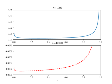
From this

$$\alpha =\frac{2K^{2}W\left(\frac{nf(K)\ln 2\ln 4}{2K^{2}}\right)}{nf(K)\ln 2\ln 4}$$

$$\approx\frac{2K^{2}}{f(K)\ln 2\ln 4}\frac{\ln n}{n},$$ (24)

where $W$ is the Lambert $W$ function.

This gives us some insight into how to choose $m$ and how DDL works. The optimum value of $\alpha$ converges to zero as $n\to\infty$. This might be somewhat surprising. In cross-validation, usually a fixed percentage of data is used for validation. If one thinks of the data $(x_{m+1},y_{m+1}),\ldots,(x_{n},y_{n})$ as ‘validation’ data in DDL, almost the entire training set is used for validation. Of course, ordinary MDL corresponds to $\alpha=0$, so in some sense this validates using MDL for machine learning. Yet, $\alpha=0$ gives an infinite error, so the take away is that the gain from DDL is to avoid this singularity. Another insight is that the optimum value of $\alpha$ increases as $K^{2}$ with the number of parameters. The factor $f(K)$ is less predictable, but at least we know it is bounded as a function of $K$. Thus, complex models require a large value of $\alpha$.

In general it of course can be difficult to find the exact optimum value of $\alpha$. However, the function in (21) is quite insensitive to $\alpha$. This is most easily seen numerically, see Fig. 1. There is a large plateau from perhaps 0.1 to 0.7 where the error is close to the minimum.

2.3 Use for model selection

Figure 2: The figure shows generalization error versus $n_{t}$ when data is dependent or independent for different values of $n$. The dots are the generalization error for full description length (MDL).

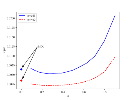
We will illustrate how the above methodology works for model selection for a simple example. The data $(x,y)$ is (iid) binary given by a conditional probability distribution $P(y|x)$ (and marginal $P_{x}(x)$). Under model $\mathcal{M}_{1}$, $y$ is independent of $x$, while under $\mathcal{M}_{2}$, $y$ is dependent on $x$. For model $\mathcal{M}_{1}$ there is a single unknown parameter $\theta_{1}=p(1|0)=p(1|1)$, while for $\mathcal{M}_{2}$ there are two unknown parameters $\theta_{2}=(p(1|0),p(1|1))$.

Fig. 2 shows the worst case regret (3) as a function of $\alpha$. The worst case regret is found by maximizing (numerically) the regret over the parameters $\theta$, $P_{x}(x)$, and the training data. The main point here, as indicated above, is that the regret is fairly insensitive to $\alpha$, and for a wide range of values of $\alpha$ the regret from DDL is smaller than MDL.

3 Hyperparameter Selection in Machine Learning

We consider a machine learning problem specified by a set of parameters $\theta_{h}$ that are estimated from the training data, and a set of hyperparameters $h$ that are chosen; the aim is to choose $h$ to minimize the generalization error (1) for log-loss (cross-entropy)

We focus on procedure 3 in Table 1, as this can be easily implemented for many ML methods and does give an actual codelength, not just an approximation. Specifically, we calculate the codelength through

$$C_{U,s}(n,(x^{n},y^{n})|m)=-\sum_{i=m}^{n-1}\log P(y_{i+1}|x_{i+1};\hat{\theta}_{h}(y^{i},x^{i}),h),$$ (25)

where $\hat{\theta}_{h}(y^{i},x^{i})$ is the maximum likelihood estimate. When $m=0$ this is Rissanen’s predictive MDL (Rissanen, 1986). An issue with predictive MDL is initialization: $\hat{\theta}_{h}(t^{i},x^{i})$ is clearly not defined for $i=0$, and likely $i$ should be large for the estimate to be good. When the initial estimate is poor, it can lead to long and arbitrary codelengths, see Sabeti and Host-Madsen (2017). An advantage of DDL is that it completely overcomes this problem because $m>0$.

3.1 Linear Regression

We can implement DDL for linear regression directly through (25). Since regression can be implemented recursively (Haykin, 2002), this is very efficient.

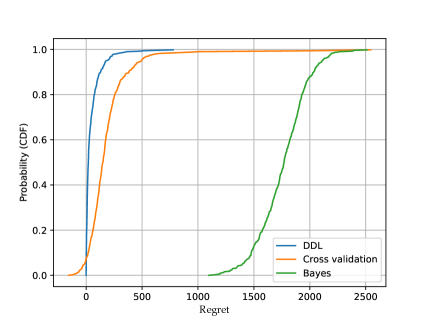
Figure 3 shows some experimental results. The setup is that of fitting polynomials of order up to 20 to the curve $\sin(3x),x\in[-2,2]$. We generate 500 random $x_{n}$ and observe $y_{n}=\sin(3x_{n})+w_{n}$, where $w_{n}\sim\mathcal{N}(0,0.15)$. We seek to optimize the regularization parameter $\lambda$ in $L_{2}$ regularization. We use DDL with $m=\frac{n}{2}$ and compare with cross-validation, where we use 25% of samples for cross-validation. We also compare with Bayes model selection, using the theory in Bishop (2006, Section 3.5.1) to optimize $\alpha=\lambda\hat{\beta}$ (notation from Bishop (2006, Section 3.5.1)). We plot the regret (3). One can see that DDL chooses the correct $\lambda$ in nearly 50% of cases, and is always better than cross-validation (The reason cross-validation can have negative regret is that $\hat{w}$ is calculated from only 75% of samples, and that has a chance of being better than an estimate calculated from the full set of training samples). It is also better than the Bayes method (which, in its defense, was not developed specifically to minimize generalization error).

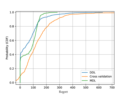
In Fig. 3 we modify the experiment to directly varying the model order $M$ without regularization. In that case, we can also compare with traditional MDL (Rissanen, 1983) through the approximation (Rissanen, 1983)

$$C_{U}(n,(x^{n},y^{n}))=\min_{\hat{\theta}_{h}}-\log P(y^{n}|x^{n};\hat{\theta}_{h},h)+\frac{M}{2}\log n$$

We see that DDL is again better than cross-validation, and better than traditional MDL, except that DDL and cross-validation have heavy tails.

(a)                                                                    (b)

Figure 3: Generalization error for least squares for simple curve fitting. The curves show the distribution of regret in terms of the CDF. (a) is for regularized LS and (b) for order selection.

3.2 Neural Networks

MDL and coding theory is based on maximum likelihood solutions e.g. in (25). On the other hand, training of a neural network is unlikely to converge to the maximum likelihood solution. Rather, the error function has many local minima, and training generally iterates to some local minimum (or a point near a local minimum), and which one can depend on the initialization condition. This requires adaption of methods like (25). Another challenge is complexity. For example, directly using predictive MDL (25) requires training for every subset of samples $(x^{i},y^{i})$ for $i=m+1,\ldots,n$, which is not computationally feasible.

Our methodology is as follows. We start with a solution $w(n)$ found by training on $(x^{n},y^{n})$; in order to implement DDL we first need another solution $w(m)$ found by training on $(x^{m},y^{m})$. We would like this solution to be “related” to $w(n)$. We therefore train on $(x^{m},y^{m})$ with $w(n)$ as initialization. The idea is that the solution for $w(m)$ will be at local minimum near $w(n)$. However, it is important that the solution $w(m)$ is independent of $((x_{m+1},y_{m+1}),\ldots,(x_{n},y_{n}))$; if not, the estimate of the generalization error will actually just be the training error. We next add the data $((x_{m+1},y_{m+1}),\ldots,(x_{n},y_{n}))$ back sequentially while retraining, in an implementation of (25); this might be done in blocks rather than for individual data points, both for reasons of efficiency and because deep learning algorithms train on data in batches. This still results in a valid coder. The idea is that we would like the sequence of solutions $w(m),w(m+1),\ldots,w(n-1)$ to converge to the original solution $w(n)$.

We test our methodology on the IMDB dataset, a real-world binary classification example, with the goal of choosing the best value for the regularization parameter $\lambda$ in $L_{2}$ regularization. This dataset contains 50,000 movie reviews which are split equally into training and test data, and each sample is labeled either as positive or negative (Maas et al., 2011). A multi-layer neural network is used to learn the data as illustrated in Fig. 4. The encoding module is a multi-hot encoder that converts the input sequences of words, restricted to top 5,000 most frequently occurring words, into a vector of 0s and 1s. Each of fully connected layers are made up of 16 neurons with ReLU activation function followed by the dropout layer with the rate of 0.5. Finally, sigmoid function is applied to map output into $[0,1]$ range.

Figure 4: Architecture of employed neural network.

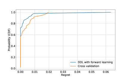
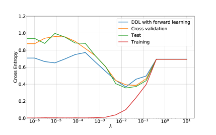
Here we compare DDL and cross-validation, where we hold out 20% of samples for cross-validation. First we do full training over $(x^{n},t^{n})$ using Adam optimizer with parameters $\alpha=0.001,\>\beta_{1}=0.9,\>\beta_{2}=0.999,\>\text{and}\>\epsilon=10^{-8}$ (Kingma and Ba, 2014). In addition, the number of total epochs and batch size are set to 50 and 128 respectively. For training over $(x^{m},t^{m})$, where $m=0.8n$, we initialize the network with weights from $(x^{n},t^{n})$ and try to unlearn holdout data. Since the gradient close to the local minima is very small, we train the network for few epochs with higher learning rate to unlearn the removed data and then switch to smaller values to learn just over $(x^{m},t^{m})$. This approach makes unlearning faster with similar complexity as training over $(x^{n},t^{n})$. For this experiment, we first train 40 epochs with learning rate $\alpha=0.01$ and then back to the initial value $\alpha=0.001$ for 10 epochs while keeping other parameters same as the training over $(x^{n},t^{n})$. We then add 5 blocks of data sequentially to retrain the network by initializing from the previous step weights. To speed up retraining, we duplicate added block multiple times until we reach the size as big as the one of the current training set. Finally, we retrain the network for only one epoch, with same parameters for training over $(x^{n},y^{n})$, which is less than 50 epochs used for training over $(x^{n},y^{n})$ and $(x^{m},y^{m})$. The codelength of sequential encoding is calculated according to the third procedure in Table 1.

We plot the regret (3), as presented in Fig. 5. The results are calculated over 50 trials where, at each trial, the training set is selected randomly from the original training dataset with the size of 20%. As it can be seen, the proposed approaches outperform cross-validation in most cases. The superiority of DDL in terms of picking the correct $\lambda$ for one typical trial is also shown in Fig. 5.

(a)                                                                    (b)

Figure 5: Generalization error for binary classification on IMDB dataset. (a) is the distribution of regret in terms of the CDF (b) is a sample of estimated generalization error by different methods vs. true generalization error.

4 Conclusion

This paper has developed the framework for DDL. We will discuss this in relation to traditional MDL. DDL can be used as a direct estimator of generalization error, which MDL cannot. Both can be used for model selection, and here we can think of DDL as a modification of MDL as follows: rather than directly using MDL for the whole dataset, we calculate the difference of MDL for the whole dataset and a subset of the data. This difference is a better decision variable than direct MDL. The difference can be calculated in three different ways, as outlined in Table 1.

References

- Alabdulmohsin [2018] Ibrahim Alabdulmohsin. Information theoretic guarantees for empirical risk minimization with applications to model selection and large-scale optimization. In Jennifer Dy and Andreas Krause, editors, Proceedings of the 35th International Conference on Machine Learning, volume 80 of Proceedings of Machine Learning Research, pages 149–158, Stockholmsmässan, Stockholm Sweden, 10–15 Jul 2018. PMLR. URL http://proceedings.mlr.press/v80/alabdulmohsin18a.html.
- Bishop [2006] Christopher M Bishop. Pattern recognition and machine learning. springer, 2006.
- Cover and Thomas [2006] T.M. Cover and J.A. Thomas. Information Theory, 2nd Edition. John Wiley, 2006.
- Grünwald [2011] Peter Grünwald. Safe learning: bridging the gap between bayes, mdl and statistical learning theory via empirical convexity. In Proceedings of the 24th Annual Conference on Learning Theory, pages 397–420, 2011.
- Grunwald [2007] Peter D. Grunwald. The Minimum Description Length Principle. MIT Press, 2007.
- Hastie et al. [2009] Trevor Hastie, Robert Tibshirani, and Jerome Friedman. The Elements of Statistical Learning, 2nd Edition. Spring, 2009.
- Haykin [2002] Simon Haykin. Adaptive Filter Theory, 4th Edition. Pearson, 2002.
- Kawakita and Takeuchi [2016] Masanori Kawakita and Jun’ichi Takeuchi. Barron and cover’s theory in supervised learning and its application to lasso. In Maria Florina Balcan and Kilian Q. Weinberger, editors, Proceedings of The 33rd International Conference on Machine Learning, volume 48 of Proceedings of Machine Learning Research, pages 1958–1966, New York, New York, USA, 20–22 Jun 2016. PMLR. URL http://proceedings.mlr.press/v48/kawakita16.html.
- Kingma and Ba [2014] Diederik P Kingma and Jimmy Ba. Adam: A method for stochastic optimization. arXiv preprint arXiv:1412.6980, 2014.
- Krichevsky and Trofimov [1981] R. Krichevsky and V. Trofimov. The performance of universal encoding. IEEE Transactions on Information Theory, 27(2):199–207, Mar 1981. ISSN 0018-9448. doi: 10.1109/TIT.1981.1056331.
- Maas et al. [2011] Andrew L Maas, Raymond E Daly, Peter T Pham, Dan Huang, Andrew Y Ng, and Christopher Potts. Learning word vectors for sentiment analysis. In Proceedings of the 49th annual meeting of the association for computational linguistics: Human language technologies-volume 1, pages 142–150. Association for Computational Linguistics, 2011.
- Rissanen [1978] Jorma Rissanen. Modeling by shortest data description. Automatica, pages 465–471, 1978.
- Rissanen [1983] Jorma Rissanen. A universal prior for integers and estimation by minimum description length. The Annals of Statistics, (2):416–431, 1983.
- Rissanen [1986] Jorma Rissanen. Stochastic complexity and modeling. The Annals of Statistics, (3):1080–1100, Sep. 1986.
- Sabeti and Host-Madsen [2017] Elyas Sabeti and Anders Host-Madsen. Enhanced mdl with application to atypicality. In 2017 IEEE International Symposium on Information Theory (ISIT). IEEE, 2017.
- Shamir [2006] G.I. Shamir. On the mdl principle for i.i.d. sources with large alphabets. Information Theory, IEEE Transactions on, 52(5):1939–1955, May 2006. ISSN 0018-9448. doi: 10.1109/TIT.2006.872846.
- Watanabe and Roos [2015] Kazuho Watanabe and Teemu Roos. Achievability of asymptotic minimax regret by horizon-dependent and horizon-independent strategies. The Journal of Machine Learning Research, 16(1):2357–2375, 2015.
- Watanabe [2013] Sumio Watanabe. A widely applicable bayesian information criterion. Journal of Machine Learning Research, 14(Mar):867–897, 2013.